Genesis of Streamwise-Localized solutions from Globally Periodic Travelling Waves in Pipe Flow

Abstract

The aim in the dynamical systems approach to transitional turbulence is to construct a scaffold in phase space for the dynamics using simple invariant sets (exact solutions) and their stable and unstable manifolds. In large (realistic) domains where turbulence can co-exist with laminar flow, this requires identifying exact localized solutions. In wall-bounded shear flows the first of these has recently been found in pipe flow, but questions remain as to how they are connected to the many known streamwise-periodic solutions. Here we demonstrate that the origin of the first localized solution is in a modulational symmetry-breaking Hopf bifurcation from a known global travelling wave that has 2-fold rotational symmetry about the pipe axis. Similar behaviour is found for a global wave of 3-fold rotational symmetry, this time leading to two localized relative periodic orbits. The clear implication is that many global solutions should be expected to lead to more realistic localized counterparts through such bifurcations, which provides a constructive route for their generation.

The transition to turbulence of wall-bounded shear flows remains a fundamental problem in fluid mechanics because of the complexity of the flows observed, the depth of the mathematical issues involved and the numerous practical implications. The central issue is that shear flows are usually linearly stable (e.g. pipe flow and plane Couette flow) yet nonlinearly unstable to small but finite-amplitude disturbances that typically trigger transition in practical situations. This transition is abrupt, immediately leading to complicated spatiotemporal flows Reynolds (1883); Emmons (1951); Bottin et al. (1998). There has, however, been considerable recent success in viewing such transitional fluid flows as large dynamical systems where transition amounts to the flow being disturbed out of the basin of attraction of the laminar shear flow Kerswell (2005); Eckhardt et al. (2007); Kawahara et al. (2012). Key to making progress with this picture has been the discovery of simple exact unstable solutions (equilibria, travelling waves, periodic orbits) to the Navier-Stokes equations Nagata (1990); Waleffe (1998); Faisst and Eckhardt (2003); Wedin and Kerswell (2004); Duguet et al. (2008), which are born in saddle node bifurcations. These solutions are either embedded in the basin boundary (between the laminar and turbulent states) or sit in the basin of attraction of the turbulent state, possibly even being buried in the turbulent attractor itself. If the turbulent state is not an attractor, the more general concept of an ‘edge’ (a codimension one hypersurface dividing initial conditions that enjoy a turbulent episode from those that immediately relaminarise) is needed. Mapping out the stable and unstable manifolds of some of these solutions embedded in the basin boundary (or edge) has revealed much about what particular disturbances are most efficient in triggering transition Pringle and Kerswell (2010); Monokrousos et al. (2011); Pringle et al. (2012) and the transition process itself Skufca et al. (2006); Schneider et al. (2007). Doing the same for solutions embedded in the turbulent attractor generates a skeleton in phase space over which the turbulent dynamics is draped Gibson et al. (2008); Willis et al. (2013).

Most of this progress has been in the context of shear flows studied over artificially small periodic domains (for theoretical convenience) where laminar and turbulent states do not co-exist and all the known exact solutions are spatially global. In real shear flows, however, transition is a spatiotemporal phenomenon where patches of turbulence are triggered that coexist with the laminar state (e.g. Reynolds, 1883; Emmons, 1951; Bottin et al., 1998). The outstanding challenge is therefore to extend this dynamical systems approach to larger domains, which naturally focuses attention on identifying localized exact solutions.

The first step in this direction was taken in plane Couette flow where spanwise-localized steady states and travelling waves were found Schneider et al. (2010a) using an edge-tracking technique Itano and Toh (2001); Skufca et al. (2006); Schneider et al. (2007). This technique identifies a relative attractor on the edge and requires it, atypically, to be a simple rather than chaotic state. Perhaps more important than discovering the states themselves was the realization (after continuing them in parameter space) that they originated in bifurcations from known global solutions, periodic in the spanwise-direction Schneider et al. (2010b). Between the local and global solutions in parameter space is a regime where the solution branch folds back and forward adding repetitions of the localized solution, termed homoclinic snaking Knobloch (2008). This suggested that further (at least) spanwise-localized versions of the catalogue of known solutions in small domains would quickly be isolated, but so far these have failed to materialize, although some progress is being made using informed guesswork Gibson and Brand (2014). To tackle the harder problem of streamwise-localization (the large streamwise flow strongly couples repetitions of the wave), the same edge-tracking technique has been employed in pipe flow to discover streamwise localisation Duguet et al. (2010), where quasi-periodic behavior was observed, and recently the first streamwise-localised simple periodic solution in shear flows Avila et al. (2013). More precisely, this is a relative periodic orbit (RPO) where the velocity field at a period later is related by a spatial shift to the initial flow. In this case no snaking behaviour was found leaving the connection back to a global state unclear.

In this Letter we discover this connection by demonstrating how the streamwise-localized solution Avila et al. (2013) arises through a symmetry-breaking bifurcation from a globally periodic state. This is important because it shows how to constructively generate further localized solutions from the numerous global states known, rather than relying on edge tracking. (This technique has been invaluable, particularly in small domains, but becomes less successful at finding exact solutions as dimension size increases e.g. with pipe length Mellibovsky et al. (2009).) To establish this connection we have traced the RPO Avila et al. (2013) towards decreasing pipe length and found a bifurcation from the N2 family of highly-symmetric travelling wave solutions Pringle et al. (2009). To investigate the prevalence of the mechanism, we show how exactly the same type of bifurcation gives rise to another (new) streamwise-localized RPO from N3, the cousin of the global travelling wave N2 with 3-fold rather than 2-fold rotational symmetry.

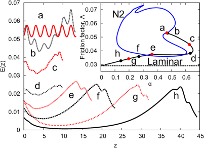
Figure 1: Localization of the bifurcation from the N2 travelling wave (three copies in $z$). Main plot: $E(z):=\int_{0}^{2\pi}d\theta\int_{0}^{1}sds\tfrac{1}{2}\mathbf{u}^{2}$ demonstrating localization along the continuation curve. Inset, continuation in $\alpha=\tfrac{2\pi}{L}$ against friction factor, $\Lambda$ (the axial pressure gradient averaged over the whole pipe and multiplied by $R/\rho U^{2}$, where $R$ is the pipe radius and $U$ the mean axial flow speed). The branch moves towards smaller domains before turning in a saddle node bifurcation and localizing. The friction factor’s linear dependence upon $\alpha$ signals localization.

Computations were carried out using a hybrid spectral finite-difference code Willis and Kerswell (2009) with a resolution of 16 Fourier modes in the azimuthal direction (so capturing up to the 32nd and 48th wavenumbers in the 2-fold and 3-fold rotational calculations respectively), 64 finite difference points in the radial direction, and 4 Fourier modes per radial length in the streamwise direction (results were checked for robustness by both increasing spatial and temporal resolution by a factor of approximately $\sqrt{2}$). The localized solution of Avila et al. (2013) was rediscovered using the edge-tracking technique Itano and Toh (2001); Skufca et al. (2006) at $Re=2200$ in a domain of length 50 pipe radii (hereon 50R). The following rotational and reflectional symmetries were imposed

$$\mathbf{R}_{m}: \left(u,v,w\right)\left(s,\theta,z\right)\rightarrow\left(u,v,w\right)\left(s,\theta+\tfrac{2\pi}{m},z\right),$$ (1)

$$\mathbf{Z}: \left(u,v,w\right)\left(s,\theta,z\right)\rightarrow\left(u,-v,w\right)\left(s,-\theta,z\right),$$ (2)

where $\left(s,\theta,z\right)$ are the usual cylindrical coordinates, $\mathbf{u}=\left(u,v,w\right)$ are the corresponding velocity components and $m$ is the order of the rotational symmetry subspace ($m=2$ here). Convergence and continuation of solutions was achieved using a Newton-Krylov-hookstep algorithm Viswanath (2007). The highly-symmetric travelling wave N2 Pringle et al. (2009) has the extra shift-&-rotate symmetry:

$$\mathbf{\Omega}_{m}:\left(u,v,w\right)\left(s,\theta,z\right)\rightarrow\left(u,v,w\right)\left(s,\theta+\tfrac{\pi}{m},z-\tfrac{\pi}{\alpha}\right)$$ (3)

where $\tfrac{2\pi}{\alpha}$ is the wavelength of the solution.

For clarity, we shall describe the bifurcation moving from the travelling wave N2 towards the localized RPO of Avila et al. (2013): see figure 1. The localized branch bifurcates as a modulational symmetry-breaking Hopf bifurcation from the N2 solution branch Pringle et al. (2009) at $\alpha_{w}\approx 1.41$. The bifurcation breaks the $\mathbf{\Omega}_{2}$ symmetry group on three copies of the underlying solution leaving a bifurcated solution with a smallest wavenumber of $\alpha=\alpha_{w}/3\approx 0.47$.

To understand the effect of breaking a symmetry in a Hopf bifurcation we consider a symmetry $C$ of order $N$. An eigenfunction, $\mathbf{u}_{1}$, breaking this symmetry satisfies $C\mathbf{u}_{1}=e^{2\pi in/N}\mathbf{u}_{1}$ where $n$ is a divisor of $N$. The new bifurcated branch can be written as $\mathbf{u}\left(t\right)=\sum_{p=-\infty}^{\infty}\epsilon^{p}\mathbf{u}_{p}e^{ip\omega t},$where $C\mathbf{u}_{0}=\mathbf{u}_{0}$ is the underlying solution, $\epsilon$ measures the distance along the branch from the bifurcation point and $\omega$ is the Hopf frequency. From the quadratic nonlinearity of the Navier-Stokes equations, the higher temporal harmonics obey $C\mathbf{u}_{p}=e^{2\pi inp/N}\mathbf{u}_{p}$ so that in the Galilean frame $z^{*}=z-ct$, where $c$ is the wavespeed of the travelling wave $\mathbf{u}_{0}(s,\theta,z^{*})$,

$$\mathbf{u}\left(\mathbf{x},t_{0}+\frac{2\pi n}{\omega N}\right) =\sum_{p=-\infty}^{\infty}\!\!\mathbf{u}_{p}e^{2\pi inp/N}e^{ip\omega t_{0}}$$

$$=\sum_{p=-\infty}^{\infty}\!\!C\mathbf{u}_{p}e^{ip\omega t_{0}}=C\mathbf{u}\left(\mathbf{x},t_{0}\right).$$ (4)

This means that the pointwise-in-time symmetry $C$ is broken down to a weaker spatiotemporal symmetry. In our specific case, $C=\Omega_{2}$, which has order $N=6$ over 3 wavelengths of $\mathbf{u}_{0}$, is broken in a Hopf bifurcation with $n=1$ down to the spatiotemporal symmetry

$$\mathbf{\Omega}_{m,\tfrac{nT}{N}}\!:\!\mathbf{u}\left(\theta,z^{*},t\right)\!\rightarrow\!\mathbf{u}\left(\theta+\tfrac{\pi}{m},z^{*}\!\!-\!\!\tfrac{\pi}{\alpha_{w}},t+\tfrac{nT}{N}\right),$$ (5)

where $T=2\pi/\omega$ (and $s$ dependence has been suppressed). This realisation is actually crucial in making the calculations possible since the RPO needs only to be traced over a time $\tau:=T/6$ rather than the full period $T$ making both the time-stepping calculations 6 times quicker and the Newton-Krylov-hookstep algorithm more likely to converge.

Continuing the RPO branch away from the bifurcation where $\tau=14.3$ (figure 1 inset) shows that the kinetic energy, $E(z)$, initially increases in one part of the domain and decreases in the other (curve b, figure 1) but then generally decreases everywhere as the domain shrinks (curve c) and then lengthens (curves d-h) with $\tau$ asymptoting to $29.8$. Examining slices of the velocity field indicates that the roll-streak structure around the energetic peak of the solution changes little from point (e) onwards but $E(z)$ near the energetic peak continues to evolve and the energetic minimum is far from zero indicating that localisation is not yet complete. For $\alpha\leq 0.2$, however, the friction factor has a linear dependence upon $\alpha$ intercepting the laminar value ($\Lambda=\tfrac{64}{Re}$) at $\alpha=0$. This linear regime indicates invariance of the solution to the domain length: the pressure gradient across the localised solution remains constant and therefore the pressure gradient averaged over the full domain scales linearly with $\alpha$.

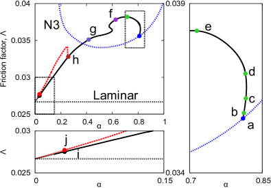
Figure 2: Continuation of the bifurcation from the N3 travelling wave (three copies in $z$) in $\alpha$ plotted against friction factor, $\Lambda$. Curve initially bifurcates towards smaller domains before turning in a saddle node; after this the solution begins to localize. At $\alpha\approx 0.26$ a secondary bifurcation breaks the $\mathbf{\Omega}_{3,T/6}$ symmetry leading to a second localized solution (plotted in red/dashed). Dots (a)-(h) correspond to solutions plotted in figure 3 and (i), (j) to those plotted in figure 4. Inset right, zoomed into region near bifurcation. Inset below, zoomed into $\alpha<0.15$ region demonstrating linear behaviour as domain length tends to infinity ($\alpha\rightarrow 0$).

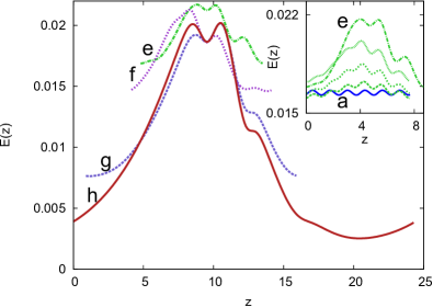
Figure 3: $E(z)$ at dots along the continuation curve (figure 2). Inset, behaviour close to the bifurcation as the solution increases in amplitude. Main, further continuation up to the secondary bifurcation as the solution localizes. Solutions (e)-(h) have been aligned to demonstrate solution evolution along the continuation curve. Solution (e) is plotted in both main & inset for comparison. Note $E(z)$ has two wavelengths to every wavelength of N3 due to the $\Omega_{2}$ symmetry (see solution (a)).

To examine whether this type of connection is generic, edge-tracking was also carried out at a similar Reynolds number and domain size ($Re=2400$, $L=50R$) but in a different rotational symmetry subspace, $\mathbf{R}_{3}$ (so $m=3$ now), while again enforcing $\mathbf{Z}$ symmetry. A localized RPO attractor within the edge is found, which can also be continued to smaller domains ending at the global periodic travelling wave N3: see figure 2. As before, the bifurcation off the N3 solution is a modulational symmetry-breaking Hopf bifurcation, on three copies of the solution, with symmetry group $\left<\mathbf{R}_{3},\mathbf{Z},\mathbf{\Omega}_{3}\right>$ at $\alpha_{w}\approx 2.43$. The $\mathbf{\Omega}_{3}$ symmetry is broken, leading to the time dependent symmetry (5) for $m=3$, $n=1$ with an initial period of $\tau=\tfrac{T}{6}=37.5$. The curve initially bifurcates towards smaller domains before rapidly turning in a saddle-node bifurcation.

Figure 3 demonstrates the rapidly changing shape of the solution during this period as $E(z)$ quickly begins to show localization. At point (h) a secondary period doubling bifurcation occurs, breaking $\mathbf{\Omega}_{3,T/6}$. Following this new branch (red curve) leads to the localized edge state. The original solution branch fully localizes but has an addition complex conjugate pair of unstable eigenvalues and is therefore not an attractor within the edge. Both solution curves enter a regime with linear dependence of friction factor on $\alpha$ as $\alpha\rightarrow 0$ indicating localization (with $\tau\rightarrow 32.9$ and $T\rightarrow 66.1$ for symmetry-maintained and symmetry-broken RPOs respectively).

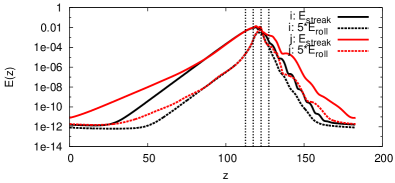
(a)

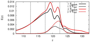
(b)

Figure 4: Energy in streaks ($\theta$-dependent streamwise flow), and rolls ($\theta$-dependent cross-stream flow) as a function of downstream position, $z$, for the two $\mathbf{R}_{3}$-symmetric localized solutions: the $\mathbf{\Omega}_{3,T/6}$ symmetric solution, labelled (i); and symmetry broken solution, labelled (j). Dotted vertical lines indicate slice locations for velocity visualization plotted in figure 5. Figure (a) Logarithm of energy, the $\mathbf{\Omega}_{3,T/6}$ symmetric solution spans approximately $120R$ including exponential tails while the symmetry-broken solution has length of approximately $180R$. Figure (b) Focused onto the centre of the domain, the amplitude of the solutions differ but have very similar roll and streak structure (not plotted).

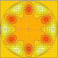
(a)

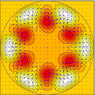
(b)

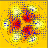
(c)

(d)

Figure 5: Flow (deviation from laminar state) at slices indicated by dotted lines in figure 4 for solution (i). Downstream flow plotted using contours with white for relatively fast flow, and red for slow flow. Arrows indicate cross-stream flow.

Formally, the solutions can only really be considered fully localized if their extremities reach the error tolerance of the code, $O\left(10^{-13}\right)$. To examine this, we took the $\mathbf{\Omega}_{3,T/6}$ symmetric localized branch and continued to $\alpha=0.035$ ($L=180R$). In figure 4 we plot the energy as a function of $z$ for the parts of the flow representing the rolls and the streaks at a point along the orbit. The $\mathbf{\Omega}_{3,T/6}$ symmetric solution, labelled (i), demonstrates the existence of exponential tails both upstream and downstream of the localized solution. The actual length of the solution can be viewed as approximately $120R$ with similar spatial decay rates for both rolls and streaks. The second localized solution within the $\mathbf{R}_{3}$ subspace, which is an attracting edge state, is also plotted (labelled (j)). While $E(z)$ differs between these solutions, the streak and roll structure of the two solutions is extremely similar. Similarities between the streak structure of these solutions and that of the lower branch N3 solution (figure 4(b) of Pringle et al. (2009)) can be observed in figure 5, with an interior wavelength corresponding to the N3 solution at $\alpha=1.25$.

In this work we have shown how the streamwise-localized RPO of Avila et al. (2013) is connected to a global highly-symmetric travelling wave N2 Pringle et al. (2009) via a simple modulational Hopf bifurcation with no snaking (i.e. successive wavelengths of the global state do not disappear at saddle node bifurcations). A further streamwise-localized RPO has been found to arise by exactly the same mechanism from N3 and yet another (more stable) RPO has been identified that bifurcates off this RPO. The implication seems clear that many more localized states undoubtedly originate via these modulational bifurcations from the wealth of spatially global states now known in shear flows. Most significantly, our results indicate that the modulational wavelength may only be 3 times longer than that of the global state. However, identifying and tracking modulational bifurcations is not guaranteed to ultimately produce a localized state. By reverse engineering, the two examples described here lead to localization but this is an inherently nonlinear behaviour that can only be determined by tracking bifurcating solution branches. However, this bifurcation approach is at least a constructive way to generate further localized solutions and so represents a systematic technique to extend the dynamical systems approach to localized turbulence and nicely complements the edge-tracking approach, which relies on being able to select a $Re$ or symmetry subspace to manufacture a simple localized edge state. Finally, it’s worth remarking that there now seems no reason why a steady modulational instability might not give rise to a steady streamwise-localised travelling wave.

References

- Reynolds (1883) O. Reynolds, Proc. R. Soc. London A. 35, 84 (1883).
- Emmons (1951) H. W. Emmons, J. Aero. Sci. 18, 490 (1951).
- Bottin et al. (1998) S. Bottin, F. Daviaud, P. Manneville, and O. Dauchot, Europhys. Lett. 43, 171 (1998).
- Kerswell (2005) R. R. Kerswell, Nonlinearity 18, R17 (2005).
- Eckhardt et al. (2007) B. Eckhardt, T. M. Schneider, B. Hof, and J. Westerweel, Annu. Rev. Fluid Mech. 39, 447 (2007).
- Kawahara et al. (2012) G. Kawahara, M. Uhlmann, and van Veen L., Ann. Rev. Fluid Mech. 44, 203 (2012).
- Nagata (1990) M. Nagata, J. Fluid Mech. 217, 519 (1990).
- Waleffe (1998) F. Waleffe, Phys. Rev. Lett. 81, 4140 (1998).
- Faisst and Eckhardt (2003) H. Faisst and B. Eckhardt, Phys. Rev. Lett. 91, 224502 (2003).
- Wedin and Kerswell (2004) H. Wedin and R. R. Kerswell, J. Fluid Mech. 508, 333 (2004).
- Duguet et al. (2008) Y. Duguet, C. C. T. Pringle, and R. R. Kerswell, Phys. Fluids 20, 114102 (2008).
- Pringle and Kerswell (2010) C. C. T. Pringle and R. R. Kerswell, Phys. Rev. Lett. 105, 154502 (2010).
- Monokrousos et al. (2011) A. Monokrousos, A. Bottaro, L. Brandt, A. Di Vita, and D. S. Henningson, Phys. Rev. Lett. 106, 134502 (2011).
- Pringle et al. (2012) C. C. T. Pringle, A. P. Willis, and R. R. Kerswell, J. Fluid Mech. 702, 415 (2012).
- Skufca et al. (2006) J. D. Skufca, J. A. Yorke, and B. Eckhardt, Phys. Rev. Lett. 96, 174101 (2006).
- Schneider et al. (2007) T. M. Schneider, B. Eckhardt, and J. A. Yorke, Phys. Rev. Lett. 99, 034502 (2007).
- Gibson et al. (2008) J. F. Gibson, J. Halcrow, and P. Cvitanovic, J. Fluid Mech. 611, 107 (2008).
- Willis et al. (2013) A. P. Willis, P. Cvitanovic, and M. Avila, J. Fluid Mech. 721, 514 (2013).
- Schneider et al. (2010a) T. M. Schneider, D. Marinc, and B. Eckhardt, J. Fluid Mech. 646, 441 (2010a).
- Itano and Toh (2001) T. Itano and S. Toh, J. Phys. Soc. Japan 70, 703 (2001).
- Schneider et al. (2010b) T. M. Schneider, J. F. Gibson, and J. Burke, Phys. Rev. Lett. 104, 104501 (2010b).
- Knobloch (2008) E. Knobloch, Nonlinearity 21, T45 (2008).
- Gibson and Brand (2014) J. Gibson and E. Brand, Journal of Fluid Mechanics 745, 25 (2014).
- Duguet et al. (2010) Y. Duguet, A. P. Willis, and R. R. Kerswell, J. Fluid Mech. 663, 180 (2010).
- Avila et al. (2013) M. Avila, F. Mellibovsky, N. Roland, and B. Hof, Phys. Rev. Lett. 110, 224502 (2013).
- Mellibovsky et al. (2009) F. Mellibovsky, A. Meseguer, T. M. Schneider, and B. Eckhardt, Phys. Rev. Lett. 103, 054502 (2009).
- Pringle et al. (2009) C. C. T. Pringle, Y. Duguet, and R. R. Kerswell, Phil. Trans. Roy. Soc. A 367, 457 (2009).
- Willis and Kerswell (2009) A. P. Willis and R. R. Kerswell, J. Fluid Mech. 619, 213 (2009).
- Viswanath (2007) D. Viswanath, J. Fluid Mech. 580, 339 (2007).