Quasars Probing Quasars VI. Excess H I Absorption within One Proper Mpc of $z\sim 2$ Quasars

Abstract

With close pairs of quasars at different redshifts, a background quasar sightline can be used to study a foreground quasar’s environment in absorption. We use a sample of 650 projected quasar pairs to study the H I Ly$\alpha$ absorption transverse to luminous, $z\sim 2$ quasars at proper separations of $30\,{\rm kpc}<R_{\perp}<1$ Mpc. In contrast to measurements along the line-of-sight, regions transverse to quasars exhibit enhanced H I Ly$\alpha$ absorption and a larger variance than the ambient intergalactic medium, with increasing absorption and variance toward smaller scales. Analysis of composite spectra reveals excess absorption characterized by a Ly$\alpha$ equivalent width profile $W=2.3\,{\rm\AA}(R_{\perp}/{\rm 100\,kpc})^{-0.46}$. We also observe a high ($\simeq 60\%$) covering factor of strong, optically thick H I absorbers (H I column $N_{\rm HI}>10^{17.3}\,{\rm cm^{-2}}$) at separations $R_{\perp}<200\,{\rm kpc}$, which decreases to $\sim 20\%$ at $R_{\perp}\simeq 1\,{\rm Mpc}$, but still represents a significant excess over the cosmic average. This excess of optically thick absorption can be described by a quasar-absorber cross-correlation function $\xi_{\rm QA}(r)=(r/r_{0})^{\gamma}$ with a large correlation length $r_{0}=12.5^{+2.7}_{-1.4}h^{-1}{\rm\ Mpc}$ (comoving) and $\gamma=1.68^{+0.14}_{-0.30}$. The H I absorption measured around quasars exceeds that of any previously studied population, consistent with quasars being hosted by massive dark matter halos $M_{\rm halo}\approx 10^{12.5}{\rm\ M}_{\odot}$ at $z\sim 2.5$. The environments of these massive halos are highly biased towards producing optically thick gas, and may even dominate the cosmic abundance of Lyman limit systems and hence the intergalactic opacity to ionizing photons at $z\sim 2.5$. The anisotropic absorption around quasars implies the transverse direction is much less likely to be illuminated by ionizing radiation than the line-of-sight, which we interpret in terms of the same obscuration effects frequently invoked in unified models of active galactic nuclei.

1. Introduction

In cold dark matter (CDM) cosmology, galaxies form within the potential wells of virialized dark matter halos where the overdensity relative to the cosmic mean exceeds $\delta\rho/\rho\gg 100$, driving gravitational collapse of gas into these halos and the subsequent formation of stars. These models also predict that the most massive galaxies arise in the highest-mass dark matter halos which, in the early Universe, trace the rarest density fluctuations. In addition, such ‘peaks’ in the density field typically occur on top of larger-scale overdensities that extend well beyond the virial radius of the collapsed halo, implying $\delta\rho/\rho\gtrsim 1$ to many Mpc. This large-scale structure is arranged in a network of filaments, sheets, clusters, etc. making up the the so-called cosmic web.

At modest overdensities $\delta\rho/\rho\lesssim 10$, the Universe’s baryons are predicted to closely track the dark matter density field. Therefore, in the vicinity of high-$z$ galaxies, the intergalactic medium (IGM) – revealed by H I Ly$\alpha$ absorption – should trace the corresponding large-scale matter distribution (e.g. Miralda-Escudé et al., 1996; Kim & Croft, 2008). Although experiments to test this paradigm are difficult to perform because surveys of high-$z$ galaxies are observationally expensive, there has been progress in the past decade. Adelberger et al. (2003) examined the mean transmission of H I Ly$\alpha$ flux through gas in the environments of the $z\sim 2-3$, star-forming Lyman break galaxies (LBGs). Aside from a peculiar behavior on the smallest scales (not confirmed by subsequent studies), they found excess H I absorption associated with LBGs on scales of a few Mpc. Crighton et al. (2011) extended this experiment to a larger dataset of quasar sightlines and LBGs; their results confirm reduced H I Ly$\alpha$ flux on scales of $2-7h^{-1}$ Mpc. Rakic et al. (2012) studied the H I Ly$\alpha$ opacity towards 15 quasars probing 679 LBGs. They reported an excess of H I Ly$\alpha$ absorption to proper impact parameters $R_{\perp}=2$ Mpc around this galactic population. Furthermore, the opacity increases with decreasing $R_{\perp}$ down to the survey limit of $\approx 50$ kpc, where the sightlines are believed to intersect the so-called circumgalactic medium (CGM). On these scales, non-linear and complex astrophysical processes related to galaxy formation may dominate the baryonic density field and the physical state of the gas (e.g. Simcoe et al., 2002; Kereš et al., 2005; Fumagalli et al., 2011b; Shen et al., 2013).

Complimentary work on the LBG-IGM connection has studied the association of individual absorption systems to these galaxies. Adelberger et al. (2005a) assessed the cross-correlation of C IV absorbers to LBGs and measured a clustering amplitude $r_{0}\approx 4h^{-1}{\rm\ Mpc}$ indicating a physical association between the metal-enriched IGM and galaxies (see also Crighton et al., 2011). Rudie et al. (2012) examined the incidence of H I absorbers at $R_{\perp}<2$ Mpc from LBGs and found systematically higher H I column densities $N_{\rm HI}$. They also concluded that the majority of $N_{\rm HI}>10^{15}\,{\rm cm^{-2}}$ absorbers may arise in the CGM of these galaxies. Altogether, these results confirm that the IGM traces the overdensities marked by luminous, star-forming galaxies at $z\sim 2-3$, supporting the concept of a cosmic web permeating the Universe between galaxies.

Galaxy formation models built on the $\Lambda$CDM hierarchical structure formation paradigm predict that more massive galaxies should occupy higher mass halos, exhibiting larger overdensities that extend to greater distances. This enhancement around massive galaxies should be reflected as signatures in the IGM absorption. In this manuscript, we test this hypothesis by focusing on the dark matter halos of galaxies hosting luminous quasars at $z\sim 2-3$. Measurements of the quasar-quasar autocorrelation function yields a correlation length of $r_{0}=8.4h^{-1}{\rm\ Mpc}$ for a projected correlation function with slope $=-1$ (White et al., 2012, see also Porciani et al. (2004); Myers et al. (2007); Shen (2009)). For a $\Lambda$CDM cosmology, this large correlation length implies a bias factor $b\approx 3.5$ and one infers that $z>2$ quasars are hosted by dark matter halos with typical mass $M_{\rm DM}\approx 10^{12.5}{\rm\ M}_{\odot}$. This correlation length and associated mass significantly exceed that measured for luminous LBGs, the best-studied, coeval galaxy population ($r_{0}^{\rm LBG}=4.0h^{-1}{\rm\ Mpc}$, $M_{\rm DM}^{LBG}\approx 10^{11.5}-10^{12}{\rm\ M}_{\odot}$; Adelberger et al., 2005b; Cooke et al., 2006b; Conroy et al., 2008; Bielby et al., 2011). Therefore, one predicts that the environments of massive galaxies hosting $z\sim 2$ quasars will exhibit stronger H I Ly$\alpha$ absorption (Kim & Croft, 2008).

On the other hand, a variety of astrophysical processes may alter this simple picture, especially on scales influenced by the galaxy and/or its neighbors (i.e. in the CGM). For example, the gas may shock to the virial temperature of the dark matter halo (i.e. $T>10^{6}$ K) which would substantially reduce the hydrogen neutral fraction. On the other hand, the galactic winds of star-forming galaxies drive a non-negligible fraction of gas and dust from their interstellar medium (ISM; e.g. Rupke et al., 2005; Shapley et al., 2003; Weiner et al., 2009; Martin et al., 2012; Rubin et al., 2013) and may therefore raise the surface density of H I gas at distances $R\gg 1$ kpc. Similarly, quasar driven outflows may inject energy and material on galactic scales, via radiative pressure and/or kinetic feedback (e.g. Moe et al., 2009; Prochaska & Hennawi, 2009). As a third example, the massive stars in the galaxy and the quasar may produce a significant flux of ionizing photons that would photoionize the surrounding gas on scales of at least tens kpc (e.g. Schaye, 2006; Chelouche et al., 2008; Hennawi & Prochaska, 2007). This proximity effect would suppress H I absorption (Bajtlik et al., 1988) but may yield a greater abundance of highly ionized gas (e.g. N V). For luminous quasars, such effects could extend to proper distances $R\gtrsim 1$ Mpc (Hennawi & Prochaska, 2007). On these scales, therefore, one may be more sensitive to the astrophysics of galaxy formation rather than the (simpler) physics of structure formation.

In this manuscript, we explore several of these processes and predictions through the analysis of H I absorption in the $R_{\perp}\leq 1$ Mpc (proper, i.e. $\approx 3h^{-1}{\rm\ Mpc}$ comoving) environments surrounding the massive galaxies tagged by $z\sim 2$ luminous quasars. This marks the sixth paper in our quasars probing quasars series, which we refer to as QPQ6. Previous work in this series introduced the novel technique of using projected quasar pairs to study quasar environments, (Hennawi et al., 2006a, QPQ1), measured the anisotropic clustering of strong H I systems around quasars (Hennawi & Prochaska, 2007, QPQ2), studied the physical conditions in the gas at $\approx 100$ kpc from a quasar (Prochaska & Hennawi, 2009, QPQ3), searched for fluorescent Ly$\alpha$ emission from optically thick absorbers illuminated by the foreground quasars (Hennawi & Prochaska, 2013, QPQ4), and characterized the circumgalactic medium of the massive galaxies hosting quasars (Prochaska et al., 2013, QPQ5). In the latter manuscript, we reported on strong H I absorption to $R_{\perp}=300$ kpc and a high covering fraction to optically thick gas (see also QPQ1 and QPQ2). This gas also shows significant enrichment of heavy elements, suggesting a gas metallicity in excess of 1/10 solar abundance (see also QPQ3). This implies a massive, enriched and cool ($T\sim 10^{4}$K) circumgalactic medium surrounding these massive galaxies, despite the presence of a luminous quasar whose ionizing flux is sufficient to severely reduce the local H I content.

Indeed, this cool CGM gas is generally not apparent along the illuminated line-of-sight. In QPQ2, we measured the incidence of strong H I absorbers in $\Delta v=\pm 1500{\rm km~{}s^{-1}}$ windows centered on the f/g quasar redshift to measure the clustering of such gas to quasars. We then used this clustering signal to predict the incidence along the quasar sightline and found it greatly exceeds the observed incidence, i.e. there is an anisotropic clustering of strong H I systems around quasars. Taken together with the general absence of fluorescent Ly$\alpha$ emission (QPQ4) from these absorbers, these observations imply that the surrounding gas observed in background sightlines is not illuminated by the foreground quasar. Such anisotropic emission follows naturally from unification models of AGN where the black hole is obscured by a torus of dust and gas (e.g. Antonucci, 1993; Elvis, 2000).

Based on the methods we have presented in the QPQ series, there is now a growing literature on the analysis of quasar pair spectroscopy to examine gas in the environments of quasar hosts. Bowen et al. (2006) searched for strong Mg II absorption at small scales ($R_{\perp}<100$ kpc) from a sample of 4 quasars at $z\sim 1$ and found a surprising 100% detection rate. Farina et al. (2013) expanded the search for Mg II absorption on small scales, also finding a high detection rate (7 of 10). They also reported on the detection of more highly ionized gas traced by the C IV doublet. These results lend further support to the concept of a cool, enriched CGM surrounding quasars. On much larger scales ($\gg 1$ Mpc), spectroscopy of quasar pairs has been analyzed to measure quasar-absorber clustering. Wild et al. (2008) measured the large-scale ($>5h^{-1}{\rm\ Mpc}$), transverse clustering of Mg II and C IV absorbers with quasars at $z\sim 1$ and 2 respectively. The clustering amplitudes ($r_{0}\approx 5h^{-1}{\rm\ Mpc}$) were used to infer that quasars are hosted by halos with masses $M>10^{12.5}{\rm\ M}_{\odot}$ at $z\sim 2$ and over $10^{13}{\rm\ M}_{\odot}$ at $z\sim 1$. These inferences assume, however, that the absorbers are unbiased tracers of the underlying dark matter density field. Most recently, Font-Ribera et al. (2013) have assessed the correlation of H I Ly$\alpha$ opacity with quasars on scales of $\approx 5-50h^{-1}{\rm\ Mpc}$. Their cross-correlation measurements confirm the results from the quasar auto-correlation function that quasars inhabit massive, dark matter halos.

At the heart of our project is a large sample of quasar pairs (Hennawi, 2004; Hennawi et al., 2006b, 2010) drawn predominantly but not exclusively from the Sloan Digital Sky Survey (Abazajian et al., 2009) and ongoing BOSS experiment (Ahn et al., 2012). We focus on projected pairs of quasars, which are physically unassociated, but project to small angular separations on the sky. In these unique sightlines, spectra of the b/g quasar are imprinted with absorption line signatures of the gas associated with the foreground (f/g) quasar. With sufficient signal-to-noise (S/N) and spectral resolution, one is sensitive to the full suite of ultraviolet diagnostics traditionally used to study the intergalactic medium: (1) H I Lyman series absorption to assess neutral hydrogen gas and by extension the underlying density field; (2) low-ion transitions of Si, C, O that track cool and metal-enriched gas; (3) high-ion transitions of C, O, and N that may trace ionized or shock-heated material associated with photoionization, virialization and/or feedback processes.

Here, we focus exclusively on H I Ly$\alpha$ absorption and defer metal-line analysis for future papers (see also QPQ3, QPQ5). As described above, our principal motivation is to trace the density field surrounding massive galaxies at $z\sim 2$ to scales of one proper and projected Mpc. The decision to cut the sample at 1 Mpc was somewhat arbitrary; we aimed to extend the analysis beyond the halo hosting the quasar but still focus on the neighboring environment. On these scales, our analysis offer constraints on the physical processes that drive the accretion of gas into dark matter halos and onto galaxies (e.g. Barkana, 2004; Faucher-Giguère & Kereš, 2011; Fumagalli et al., 2011b). Models of these processes are still in a formative stage and exploring trends with mass and redshift offer valuable insight.

Our experiment uses luminous quasars as a signposts for distant massive dark matter halos. Because quasar activity represents a brief energetic phase of galaxy evolution, our results could show peculiarities related to quasar activity, which are not representative of the massive halo population as a whole. Ionizing radiation from the quasar, for example, may photoionize gas in the surrounding environment on scales to 1 Mpc and beyond, imposing a so-called transverse proximity effect (TPE). Work to date, however, has not shown strong evidence for such an effect (Croft, 2004; Kirkman & Tytler, 2008); in fact (as noted above), we have identified excess H I absorption on scales of the CGM (QPQ2, QPQ5). Quasars may also drive outflows, frequently invoked to suppress star-formation and/or remove the cold ISM of massive galaxies, which would inject energy and material into the surrounding medium. Indeed, a high incidence of metal-line absorption is observed in the CGM of quasars (QPQ3,QPQ5 Bowen et al., 2006; Farina et al., 2013). In these respects, therefore, our experiment also offers insight into processes of quasar feedback on scales of tens kpc to 1 Mpc.

This paper also describes the methodology, sample selection, data collection, reduction, and quasar redshift and continua measurements of our ongoing program. As a result, this is a lengthy manuscript intended to provide a nearly complete description of the methodology and our program’s assessment of H I gas on 1 Mpc scales. The casual reader, therefore, may wish to focus his/her attention on $\S$ 6 which discusses the key results and their implications. The full paper is organized as follows: In $\S$ 2, we describe detail the spectral datasets that comprise QPQ6 including data reduction, continuum normalization, and quasar redshift measurements. Non-parametric measurements of the H I absorption are presented in $\S$ 3. Measurements of the equivalent width and H I column densities are given in $\S$ 4. We generate and analyze composite spectra at H I Ly$\alpha$ in $\S$ 5. In $\S$ 6, we discuss the main results and draw inferences. We conclude with a summary of the main findings in $\S$ 7. Throughout this manuscript, we adopt a $\Lambda$CDM cosmology with $\Omega_{M}=0.26,\Omega_{\Lambda}=0.74$, and $H_{0}=70{\rm km\,s^{-1}\,Mpc}$. In general, we refer to proper distances in units of Mpc. The primary exception is in the clustering analysis of § 6.4 where we employ comoving distances in units of $h^{-1}{\rm\ Mpc}$ for consistency with the conventions used in clustering.

2. Data and Preparation

In this section, we discuss the criteria that define the QPQ6 sample and the corresponding, diverse spectroscopic dataset that forms the basis of analysis for this QPQ6 manuscript. We also describe several procedures required to prepare the data for absorption-line analysis.

2.1. Experimental Design and the QPQ6 Sample

The primary goal of this paper is to explore the H I Ly$\alpha$ absorption of the environment surrounding $z\sim 2.5$ quasars on proper scales of 10 kpc to 1 Mpc. To accomplish this goal, we utilize projected quasar pairs. Analysis of the absorption-line spectroscopy for the background (b/g) quasar diagnoses the gas (in projection) associated to a foreground (f/g) quasar. To effectively probe a wide dynamic range in projected radii, we have leveraged several large spectroscopic survey datasets and have performed dedicated follow-up observations on a number of large-aperture telescopes. For the former, we use the spectroscopic quasar databases of the Sloan Digital Sky Survey (SDSS; Abazajian et al., 2009) and the recently released Baryonic Oscillation Spectroscopic Survey data release 9 (DR9) (BOSS Ahn et al., 2012). For the latter, we have collected follow-up observations of quasar pairs from the Keck, Magellan, Gemini, and the Large Binocular Telescope.

The starting point of our experiment is to discover projected quasar pairs with angular separation $\theta$ corresponding to proper separations of $R_{\perp}<1$ Mpc. Modern spectroscopic surveys select against close pairs of quasars because of fiber collisions. For the SDSS and BOSS surveys, the finite size of their optical fibers preclude discovery of pairs with separation $<55\arcsec$ and $<62\arcsec$, corresponding respectively to to 414 kpc and 467 kpc at $z=2$. At $z=2$, however, our target separation of $<1$ Mpc corresponds to $\theta<2.1^{\prime}$, which exceeds the fiber collision scale of these surveys. Therefore, these survey datasets provide a large sample of quasar pairs for $R_{\perp}\gtrsim 500$ kpc, but relatively few at smaller separations. In the regions where spectroscopic plates overlap, this fiber collision limit can be circumvented. However, presently only $\approx 30\%$ of the SDSS spectroscopic footprint and $\approx 40\%$ of the BOSS footprint are in overlap regions. Unfortunately, small separation quasar pairs are rare, and only a small fraction of the of SDSS/BOSS spectra from overlapping plates have sufficient data quality to meet our analysis criteria.

To better sample the gas surrounding quasars at small $R_{\perp}$, we have been conducting a comprehensive spectroscopic survey to discover additional close quasar pairs and to follow-up the best examples for our scientific interests. Close quasar pair candidates are selected from a photometric quasar catalog (Bovy et al., 2011, 2012), and are confirmed via spectroscopy on 4m class telescopes including: the 3.5m telescope at Apache Point Observatory (APO), the Mayall 4m telescope at Kitt Peak National Observatory (KPNO), the Multiple Mirror 6.5m Telescope, and the Calar Alto Observatory (CAHA) 3.5m telescope. Our continuing effort to discover quasar pairs is described in Hennawi (2004), Hennawi et al. (2006b), and Hennawi et al. (2010). Projected pair sightlines were then observed with 8m-class telescopes at the Keck, Gemini, MMT, Magellan, and LBT observatories to obtain science-grade, absorption-line spectra. Over the years, we have had various scientific goals when conducting the follow-up spectroscopy. This includes measuring the small-scale clustering of quasars (Hennawi et al., 2006b; Shen et al., 2010; Hennawi et al., 2010), exploring correlations in the IGM along close-separation sightlines (Ellison et al., 2007; Martin et al., 2010), analyzing small-scale transverse Ly$\alpha$ forest correlations (Rorai et al., 2013), characterizing the transverse proximity effect (Hennawi et al.  in prep), and using the b/g sightline to characterize the circumgalactic medium of the f/g quasar (our QPQ series). Only the latter effort is relevant to this paper.

We emphasize that the nature of previously measured absorption at H I Ly$\alpha$ for the f/g quasar very rarely influenced the target selection. Therefore, the overall dataset has no explicit observational bias regarding associated H I absorption. The diverse nature of our scientific programs and evolving telescope access, however, has led to a follow-up dataset which is heterogeneous in terms of spectral resolution ($R\approx 1000-40,000$), S/N, and wavelength coverage. From the master dataset, we generated the QPQ6 sample as described below. A discussion of the spectroscopic observations and data reduction procedures are given in the following sub-section.

The parent sample is all unique, projected quasar pair sightlines which have a proper transverse separation of $R_{\perp}<1\,{\rm Mpc}$ at the redshift of the f/g quasar. The initial list of potential quasar pair members includes any known systems, irrespective of the survey design or spectroscopic characteristics. This includes all of the quasars in the SDSS (Schneider et al., 2010), 2QZ (Croom et al., 2004) and BOSS (Pâris et al., 2012) samples, all the quasars confirmed from our 4m telescope follow-up targeting quasar pairs, and any quasars discovered during our observations on large-aperture telescopes. For the following analysis, we have further restricted to pairs where each member has either an SDSS, BOSS, or large-aperture telescope science spectrum of the b/g quasar.

An initial cut on velocity difference between the redshifts of the two quasars of $\Delta v>2000{\rm km~{}s^{-1}}$ was made to minimize confusion between physically unassociated projected pairs and physically associated binary quasars. For physical binaries, it is impossible to distinguish absorption intrinsic to the background quasar from absorption associated with the foreground quasar. Strong broad absorption line (BAL) quasars with large C IV equivalent widths (EWs) were excluded from the analyses, if apparent in either the f/g or b/g quasar. Mild BALs were excluded if BAL absorption in the b/g quasar coincided with Ly$\alpha$ of the f/g quasar redshift or if BAL absorption precluded a precise redshift estimate of the f/g quasar. This yielded a parent sample of over 2000 quasars pairs with proper separation at the f/g quasar of $R_{\perp}\leq 1$ Mpc.

We further require that the wavelength of the f/g quasar’s Ly$\alpha$ line,

$$\lambda_{\rm Ly\alpha}^{\rm fg}=(1+z_{\rm fg})\,1215.6701{\rm\AA}\;\;\;,$$ (1)

lie within the wavelength coverage of the b/g spectrum, and at a velocity corresponding to 500  km s^-1 blueward of the b/g quasar’s Ly$\beta$ emission line. The latter criterion is a first, lenient cut to avoid Ly$\alpha$ absorption being confused with higher order Lyman series lines. We impose a stricter cut after re-measuring the f/g quasar redshift (see below). In the b/g quasar spectrum, we measured the average signal-to-noise per rest-frame Å in a $\pm 500{\rm km~{}s^{-1}}$ window centered on $\lambda_{\rm Ly\alpha}^{\rm fg}$, ${\rm S/N}_{\rm Ly\alpha}$. This ${\rm S/N}_{\rm Ly\alpha}$ ratio is measured from an estimated continuum for the b/g quasar not the absorbed flux. If no continuum had been generated in the pursuit of previous analyses (e.g. QPQ5), we used the algorithm developed by Lee et al. (2012) to measure quasar continua for SDSS and BOSS spectra (see $\S$ 2.3.1 for details). All pairs with ${\rm S/N}_{\rm Ly\alpha}>4.5$ were passed through for further consideration. We also visually inspected the spectra with ${\rm S/N}_{\rm Ly\alpha}<4.5$ and passed through those cases where the automated algorithm had failed to generate a sensible continuum.

Figure 1.— These panels summarize key properties of the QPQ6 quasar pair dataset as a function of pair separation $R_{\perp}$ (projected and proper, measured at the f/g quasar redshift). The f/g quasars have redshifts predominantly at $z_{\rm fg}=2-3$ and Bolometric luminosities $L_{\rm Bol}=10^{46}-10^{47}\,{\rm erg\,s^{-1}}$. Assuming isotropic emission and a distance equal to the impact parameter, we estimate enhancements in the UV flux relative to the EUVB of $g_{\rm UV}=10-10,000$ scaling inversely with $R_{\perp}^{2}$. Lastly, the signal-to-noise of the b/g spectrum at Ly$\alpha$ of the f/g quasar ($\lambda_{\rm Ly\alpha}^{\rm fg}$) ranges from 5.5 (the QPQ6 cutoff) to over 100 per rest-frame Å.

For the pairs that survived these cuts, we re-analyzed the f/g quasar spectrum to measure a more precise emission redshift $z_{\rm fg}$ (see $\S$ 2.3.2 for details). Note that this is the only analysis performed on the f/g quasar spectrum in this manuscript. This cut on redshift quality eliminated $\approx 25\%$ of the pairs. Using these revised redshifts, we recorded the velocity offset between $\lambda_{\rm Ly\alpha}^{\rm fg}$ and Ly$\beta$ of the b/g quasar and demanded a separation of $1500{\rm km~{}s^{-1}}$ (to the red). Similarly, we further restrict the sample to pairs where the velocity difference between the new f/g quasar redshifts and the b/g redshift exceeds 4000  km s^-1. This insures the quasars are projected and should minimize the impact from the proximity region of the b/g quasar. Next, we generated a continuum for any b/g quasar spectrum without one or with a poor estimation from the automated algorithm ($\S$ 2.3.1). Lastly, we re-measured ${\rm S/N}_{\rm Ly\alpha}$ and required that it exceed 5.5 per rest-frame Å. This criterion is a compromise between maximizing sample size versus maintaining a high-level of data quality on the individual sightlines. We adopt even stricter criteria on ${\rm S/N}_{\rm Ly\alpha}$ for several of the following analyses. Lastly, we identified a small set ($\approx 30$) of pairs where the b/g quasar spectrum was compromised by insufficient wavelength coverage, a detector gap, or previously unidentified BAL features. These quasars were eliminated from any further consideration.

Table 1QPQ6 Survey

f/g Quasar	$z_{\rm fg}^{a}$	$L_{\rm 912}^{b}$	$L_{\rm Bol}$b	b/g Quasar	$z_{\rm bg}$	$R_{\perp}$	$g_{\rm UV}$b
		(cgs)	(cgs)			(kpc)
J000211.76$-05$2908.4	2.8190	30.46	46.49	J000216.66$-05$3007.6	3.147	768	65
J000426.43$+00$5703.5	2.8123	29.96	46.00	J000432.76$+00$5612.5	2.920	882	17
J000536.29$+00$0922.7	2.5224	30.38	46.42	J000531.32$+00$0838.9	2.848	725	57
J000553.32$-03$1200.3	2.5468	29.87	45.91	J000551.25$-03$1104.7	3.058	533	33
J000629.92$-00$1559.1	2.3327	29.79	45.85	J000633.35$-00$1453.3	2.882	711	16
J000839.31$-00$5336.7	2.6271	30.70	46.71	J000838.30$-00$5156.7	2.887	841	89
J001028.78$-00$5155.7	2.4268	29.87	45.89	J001025.73$-00$5155.3	2.800	387	61
J001247.12$+00$1239.4	2.1571	30.59	46.64	J001250.49$+00$1204.0	2.203	532	164
J001351.21$+01$2717.9	2.2280	…	…	J001357.14$+01$2739.2	2.303	784	…
J001605.88$+00$5654.2	2.4021	30.15	46.28	J001607.27$+00$5653.0	2.598	176	558

Note. — [The complete version of this table is in the electronic edition of the Journal. The printed edition contains only a sample.]

The final QPQ6 sample comprises 650 pairs at $z_{\rm fg}>1.6$ with $R_{\perp}<1$ Mpc. Figure 1 presents a series of plots summarizing the demographics of the f/g quasars and the spectral quality; Table 1 lists these properties. From $R_{\perp}\approx 30-500$ kpc we have a fairly uniform sampling of impact parameters. Beyond 500 kpc, where we are no longer limited by fiber collisions, the sample is dominated by BOSS spectroscopy and the f/g quasars tend toward higher redshift and the number of pairs per $R_{\perp}$ interval increases with separation. Nevertheless, there is no strong dependence on the bolometric luminosity with $R_{\perp}$. The values range from $10^{45.5-47}$ erg s^-1, where we have combined SDSS $i$-band photometry and the McLure & Dunlop (2004) relation to convert magnitudes to bolometric luminosities. If these sources are shining at near the Eddington limit (we adopt 10% as a fiducial value), they correspond to black holes with masses of $\gtrsim 10^{9}{\rm\ M}_{\odot}$ (Shen et al., 2011).

The specific luminosities at 1 Ryd ($L_{912}$) were estimated from the quasar redshift and the SDSS photometry (Hennawi et al., 2006a), and they range from $10^{29.5}-10^{31.2}{\rm erg\ s^{-1}\ Hz^{-1}cm^{-2}}$. This implies an enhancement in the radiation field by the quasar relative to the extragalactic UV background at 100 kpc (1 Mpc) of $g_{\rm UV}\approx 1000(10)$ (see QPQ1 for how $g_{\rm UV}$ is computed).

The quasar pair sample presented in QPQ5 is a subset of the QPQ6 dataset, restricted to have $R_{\perp}\leq 300$ kpc to isolate the CGM, ${\rm S/N}_{\rm Ly\alpha}>9.5$, and further restricted to SDSS, BOSS-DR9, Keck/LRIS, Gemini/GMOS data taken prior to 2011, and any of our Magellan observations.

2.2. Spectroscopic Observations

Our analysis draws on several datasets to explore the H I absorption associated with $z\sim 2$ quasars. In practice, we have utilized at least two spectra per pair: one to measure the redshift of the f/g quasar and another to gauge the H I Ly$\alpha$ absorption in the spectrum of a b/g quasar. A majority of the sources rely on spectra from the SDSS DR7 (Abazajian et al., 2009) and BOSS DR9 (Ahn et al., 2012) surveys, which have spectral resolution $R\approx 2000$ and wavelength coverage from $\lambda\approx 3800-9000$Å and $\lambda\approx 3600-10000$Å  respectively. We refer interested readers to the survey papers for further details.

Table 2Journal of Observations

b/g Quasara	Obs.	Instr.b	Datec	Exp. (s)d
J002802.60$-10$4936.0	Keck	ESI	2008-07-04	3600
J022519.50$+00$4823.7	Keck	ESI	2005-11-28	7100
J022519.50$+00$4823.7	Keck	ESI	2005-11-28	7100
J081806.87$+07$1920.2	Keck	ESI	2006-11-18	1800
J102616.11$+46$1420.8	Keck	ESI	2008-01-04	3600
J103900.01$+50$2652.8	Keck	ESI	2008-01-04	2000
J121533.54$-03$0925.1	Keck	ESI	2007-04-12	10800
J131428.97$+28$1840.2	Keck	ESI	2008-07-04	2400
J154225.81$+17$3322.9	Keck	ESI	2008-06-05	3000
J155952.67$+19$2310.5	Keck	ESI	2008-07-04	1800

Note. — [The complete version of this table is in the electronic edition of the Journal. The printed edition contains only a sample.]

Our QPQ survey has been gathering follow-up optical spectra on large-aperture telescopes using spectrometers with a diverse range of capabilities. This includes data from the Echellette Spectrometer and Imager (ESI; Sheinis et al., 2002), the Low Resolution Imaging Spectrograph (LRIS; Oke et al., 1995), and the High Resolution Echelle Spectrometer (HIRES; Vogt et al., 1994) on the twin 10m Keck telescopes, the Gemini Multi-Object Spectrograph (Hook et al., 2004, GMOS;) on the 8m Gemini North and South telescopes, the Magellan Echellette Spectrograph (MagE; Marshall et al., 2008) and the Magellan Inamori Kyocera Echelle (MIKE; Bernstein et al., 2003) spectrometers on the 6m Magellan telescopes, and the Multi-Object Double Spectrograph (MODS; Pogge et al., 2012) on the Large Binocular Telescope (LBT). A summary of all these observations is provided in Table 2.

At the W.M. Keck Observatory, we have exploited three optical spectrometers to obtain spectra of quasar pairs. For the Keck/LRIS observations, we generally used the multi-slit mode with custom designed slitmasks that enabled the placement of slits on other known quasars or quasar candidates in the field. LRIS is a double spectrograph with two arms giving simultaneous coverage of the near-UV and red. We used the D460 dichroic with the $1200$ lines mm^-1 grism blazed at $3400$ Å on the blue side, resulting in wavelength coverage of $\approx 3300-4200$ Å, a dispersion of $0.50$ Å per pixel, and the $1^{\prime\prime}$ slits give a FWHM resolution of $125{\rm km~{}s^{-1}}$. These data provide the coverage of Ly$\alpha$ at $z_{\rm fg}$. On the red side we typically used the R600/7500 or R600/10000 gratings with a tilt chosen to cover the Mg II emission line at the f/g quasar redshift, useful for determining accurate systemic redshifts of the quasars (see § 2.3.2). Occasionally the R1200/5000 grating was also used to give additional bluer wavelength coverage. The higher dispersion, better sensitivity, and extended coverage in the red provided high signal-to-noise ratio spectra of the Mg II emission line and also enabled a more sensitive search for metal-line absorption in the b/g quasar (see Prochaska et al. in prep.). Some of our older data also used the lower-resolution 300/5000 grating on the red-side covering the wavelength range $4700-10,000$ Å. About half of our LRIS observations were taken after the atmospheric dispersion corrector was installed, which reduced slit-losses (for point sources) in the UV. The Keck/LRIS observations took place in a series of runs from 2004-2008. Keck/HIRES observations ($R\approx 35,000$) were taken for one pair in the sample; these observations and data reduction were described QPQ3. Keck/ESI observations ($R\approx 5,000$) were obtained for 12 pairs covering Ly$\alpha$ in the QPQ6 sample. These data have been previously analyzed for C IV correlations between neighboring sightlines (Martin et al., 2010) and for the analysis of an intriguing triplet of strong absorption systems (Ellison et al., 2007). We refer the reader to those papers for a full description of the data acquisition and reduction.

The Gemini data were taken with the GMOS on the Gemini North and South facilities. We used the B$1200\_G5301$ grating which has 1200 lines mm^-1 and is blazed at 5300 Å. The detector was binned in the spectral direction resulting in a pixel size of 0.47 Å, and the $1\arcsec$ slit corresponds to a FWHM $\simeq 125{\rm km~{}s^{-1}}$. The slit was rotated so that both quasars in a pair could be observed simultaneously. The wavelength center depended on the redshift of the quasar pair being observed. We typically observed $z\sim 2.3$ quasars with the grating centered at 4500 Å, giving coverage from $3750-5225$ Å, and higher redshift $z\sim 3$ pairs centered at 4500 Å, covering $4000-5250$ Å. The Gemini CCD has two gaps in the spectral direction, corresponding to 9 Å at our resolution. The wavelength center was thus dithered by 15-50Å between exposures to obtain full wavelength coverage in the gaps. The Gemini North observations were conducted over three classical runs during UT 2004 April 21-23, UT 2004 November 16-18, and UT 2005 March 13-16 (GN-2004A-C-5, GN-2004B-C-4, GN-2005A-C-9, GN-2005A-DD-4). We are also pursuing a new project to study the CGM of damped Ly$\alpha$ systems (unassociated with the f/g quasar) which began in Semester 2012A on Gemini South (GN-2012A-Q-12), and is continuing on Gemini North and South (GN-2012-B-Q-12 and GS-2012-B-Q-20). These data were taken with a $0.5^{\prime\prime}$ wide longslit using the B600_G5307 grating yielding a FWHM $\approx 125{\rm km~{}s^{-1}}$ spectral resolution. We employed two central wavelengths covering $3600-6270$Å and $4350-7150$Årespectively. The data presented here were taken prior to August 20, 2012, and are thus restricted to the GN-2012A-Q-12 program only.

Observations of 13 pairs were obtained with the Magellan telescopes using the MagE and MIKE spectrometers. These data have spectral resolution $R=4,000$ for MagE and $R=28,000$ ($R=22,000$) for blue (red) side of MIKE. The wavelength coverage of the MagE instrument is fixed at $\lambda\approx 3050-10300$Å and we observed with MIKE in its standard configuration giving $\lambda\approx 3300-9150$Å. MagE data were obtained on the nights of UT 2008 January 07-08, UT 2008 April 5-7, and UT 2009 March 22-26, whereas MIKE data was obtained only on the latter observing run.

We have a complementary program to study the CGM of DLAs using the MODS spectrometer on the LBT. Our current sample includes 5 pairs from that survey. Each was observed with a $0.6^{\prime\prime}$ longslit oriented to include each member of the pair. The blue camera was configured with the G400L grating giving a FWHM $\approx 200{\rm km~{}s^{-1}}$ spectral resolution and the red camera used the G670L grating giving FWHM $\approx 200{\rm km~{}s^{-1}}$. Together the data span from $\lambda\approx 3000-10000$Å.

All of the follow-up spectra that our team acquired were reduced with custom IDL data reduction pipelines (DRPs) developed primarily by J. Hennawi and J.X. Prochaska and are publicly available and distributed within the XIDL software package. We refer the interested reader to the paper describing the MagE pipeline (Bochanski et al., 2009) which summarizes the key algorithms employed in all of the DRPs. In short, the spectral images are bias subtracted, flat-fielded, and wavelength calibrated, and the codes optimally extract the data producing a calibrated (often fluxed) 1D spectrum. We estimate a $1\sigma$ uncertainty vector for each co-added spectrum based on the detector characteristics, sky spectrum, and the measured RMS in multiple exposures. Wavelength calibration was always performed using calibration arc lamps and frequenly corrected for instrument flexure using sky emission lines. Uncertainties in this calibration are less than one-half binned pixel, i.e. less than 35  km s^-1 for all of the spectra. Such error does not contribute to uncertainty in any o the analysis that follows. A set of representative spectra are shown in Figure 2.

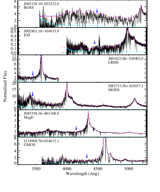
Figure 2.— A set of representative spectra of the b/g quasars in the QPQ6 dataset. The data are plotted in the observer reference frame and the blue arrows indicate the position of Ly$\alpha$ for the f/g quasar, $\lambda_{\rm Ly\alpha}^{\rm fg}$. The cyan dash-dotted line traces the $1\sigma$ error array. The dotted red line traces the original continuum, while the dashed purple line shows the mean-flux regulated (MFR) continuum (see $\S$ 2.3.1 for definitions).

2.3. Preparation for the H I Ly$\alpha$ Analysis

2.3.1 Continuum Normalization

An assessment of the H I Ly$\alpha$ absorption requires normalization of the b/g quasar spectrum at $\lambda_{\rm Ly\alpha}^{\rm fg}$. In addition, control measures of H I absorption are performed on ‘random’ spectral regions throughout the data; this also requires normalized spectra. Therefore, we have estimated the quasar continuum at all wavelengths blueward of the N V emission line for each of the b/g quasar spectra in the QPQ6 dataset.

We have generated two estimates of the continuum for each b/g quasar spectrum in QPQ6 with the following recipe. First, for each spectrum which covered both the Ly$\alpha$ forest and the C IV emission-line of the b/g quasar, we used the Principal Component Analysis (PCA) algorithm developed by K.G. Lee (Lee et al., 2012) to generate a continuum. The Lee algorithm generates a quasar SED based on a PCA analysis of the data redward of Ly$\alpha$ and then modulates this SED by a power-law so that the transmitted flux at rest-frame wavelengths $\lambda=1040-1180$Å best matches the mean transmission of the IGM measured by Faucher-Giguère et al. (2008c). This latter treatment is referred to as mean-flux regulation. In the version of the code available to the lead author at the time, there was no masking of strong absorption lines (e.g. DLAs) along the sightlines. Therefore, this first estimate often showed regions of the continuum that were biased too low. Similarly, stochasticity in the Ly$\alpha$ forest means that some spectra have significantly lower/higher Ly$\alpha$ absorption than the average, which biases the continuum for that individual quasar. To mitigate these effects, one of us (JXP) visually inspected each continuum and re-normalized the estimate when it was obviously required (e.g. the continuum lies well below the observed flux). In some cases an entirely new continuum was required, and in all cases the continuum was extended to longer and shorter wavelengths than the region fitted by the Lee algorithm. These modifications to the continuum were done by-hand, using a spline algorithm.

A spline algorithm was also adopted for the spectra where the Lee algorithm could not be applied or where it failed. One of us (JXP) generated a spline function by-hand that traces the obvious undulations and emission features of the b/g quasar. These features, of course, are more easily discerned in the higher $S/N$ spectra. This led, in part, to the imposed ${\rm S/N}_{\rm Ly\alpha}$ criterion of the QPQ6 sample. At the typical spectral resolution of our QPQ6 sample, one generally expects the normalized flux to lie below unity (in the absence of noise) owing to integrated Ly$\alpha$ opacity from the IGM. We took this into full consideration when generating the spline continuum and also allowed for the expected increase in Ly$\alpha$ opacity with increasing redshift.

At the end of this first stage, we had generated a continuum for every spectrum of the b/g quasars in the QPQ6 sample. In the following, we refer to this set of continua as the ‘Original’ continua. These were applied to the data to estimate S/N and to perform the line-analysis in $\S$ 4. For all other analyses, we modulated these original continua as follows. First, any BOSS spectrum was renormalized by the Balmer flux correction recommended for these data (Lee et al., 2013). Second, we mean-flux regulated every original continuum following the Lee et al. (2012) prescription, i.e. by solving for the power-law that best matches the mean flux of the IGM estimated by Faucher-Giguère et al. (2008c):

$$<F>_{\rm IGM}=\exp(-\tau_{\rm IGM})\;\;{\rm with}\;\tau_{\rm IGM}=0.001845(1+z)^{3.924}\;\;\;.$$ (2)

In this analysis, we have masked the $\pm 50$Å region surrounding Ly$\alpha$ of the f/g quasar and $\pm 100$Å around strong Ly$\alpha$ absorbers (primarily DLAs) given by Lee et al. (2013) and our own visual inspection (Rubin et al.  in prep.). The derived power-law was then applied to the original continuum at all wavelengths $\lambda_{r}<1220$Å in the rest-frame of the b/g quasar. We refer to this second set as the “Mean-Flux-Regulated (MFR)” continua.

Figure 2 shows the original and MFR continua on the sample of representative data. We estimate the average uncertainty in the continuum to be $\approx 5-10\%$ (dependent on S/N), improving to a few percent outside the Ly$\alpha$ forest. The majority of this error is systematic (e.g. poorly modeled fluctuations in the quasar emission lines), but such errors should be uncorrelated with properties of the f/g quasars. And, we reemphasize that we have masked the spectral region near the f/g quasar when performing the mean-flux regulation to avoid it from influencing the result.

Table 3QPQ6 Quasar Redshifts

f/g Quasar	Spect	Lines	$z_{\rm em}$	$\sigma_{z}$
				(  km s-1)
J000211.76$-05$2908.4	SDSS	SiIV,CIV, [CIII]	2.8190	520
J000426.43$+00$5703.5	BOSS	SiIV	2.8123	792
J000536.29$+00$0922.7	BOSS	MgII	2.5224	272
J000553.32$-03$1200.3	BOSS	SiIV, CIV	2.5468	714
J000629.92$-00$1559.1	BOSS	CIV	2.3327	794
J000839.31$-00$5336.7	BOSS	SiIV,CIV, [CIII]	2.6271	520
J001028.78$-00$5155.7	BOSS	CIV	2.4268	794
J001247.12$+00$1239.4	SDSS	SiIV,CIV, [CIII]	2.1571	520
J001351.21$+01$2717.9	BOSS	CIV	2.2280	794
J001605.88$+00$5654.2	BOSS	CIV, [CIII]	2.4021	653

Note. — [The complete version of this table is in the electronic edition of the Journal. The printed edition contains only a sample.]

2.3.2 Redshift Analysis

The redshifts used for the initial selection of quasar pairs were taken from the SDSS or BOSS catalogs. The methodology used by those projects, detailed in Schneider et al. (2010); Pâris et al. (2012), is to fit a quasar template to the observed spectrum and solve for the emission redshift $z_{\rm em}$. It is now well-recognized, however, that these redshifts are not optimal and may even have a significant and systematic offset from the systemic redshift of the quasar’s host galaxy (Shen et al., 2007; Hewett & Wild, 2010; Font-Ribera et al., 2013).

For our analysis of quasar pairs, the results are most sensitive to the systemic redshift adopted for the f/g quasar. We aim to associate the source with H I absorption which shows significant variations on scales of $100{\rm km~{}s^{-1}}$ in the $z\sim 2$ IGM. Therefore, we have refined the SDSS/BOSS redshift measurements as follows. Our methodology uses the custom line-centering algorithm described in QPQ1 to determine the line-center of one or more far-UV emission lines (Mg II, [C III], Si IV, C IV). We then use the recipe in Shen et al. (2007) for combining these measurements from different emission lines. We center all emission lines with $S/N>5$ covered by our spectroscopic dataset. These data, of course, are distinct from the spectra of the b/g quasars and may not even include the f/g quasar’s Ly$\alpha$ line. The specific spectrum and emission-lines analyzed are listed in Table 3. When it is available, we adopt the redshift estimated from Mg II alone because its offset from systemic is the smallest and it also exhibits the smallest scatter about systemic (after applying the offset; Richards et al., 2002). We cover Mg II emission for many of the f/g quasars in the QPQ6 sample having $z_{\rm fg}<2.4$ ($\approx 40\%$), and we assume a $1\sigma$ uncertainty of $272{\rm km~{}s^{-1}}$ following Richards et al. (2002).

In lieu of Mg II, we analyze one or more of the remaining emission lines depending on the wavelength coverage and $S/N$ of the spectra. If none of the lines could be analyzed, the pair has not been included here. The precision assumed for $z_{\rm em}$ depends on which lines were analyzed (Table 3; Richards et al., 2002) and is in the range of $\sigma(z_{\rm em})\simeq 270-770{\rm km~{}s^{-1}}$ All of the automated fits were inspected by-eye and minor modifications were occasionally imposed (e.g. eliminating a blended or highly-absorbed line from the analysis).

We measure an average offset between $z_{\rm em}$ and $z_{\rm orig}$ of $\Delta v\approx+390{\rm km~{}s^{-1}}$, which is due to a systematic offset results from the redshift determination algorithm used by the SDSS survey survey (Richards et al., 2002; Hewett & Wild, 2010). Font-Ribera et al. (2013) report a similar offset based on their analysis of quasar clustering with the Ly$\alpha$ forest. There is no strong redshift dependence for $\Delta v$ aside from larger uncertainties at higher $z$ where the spectra no longer cover the Mg II emission line. We proceed with the analysis using these new estimates for the redshifts (tabulated in Table 3). For the systems with $z_{\rm em}$ values derived from Mg II emission, the precision ($\approx 270{\rm km~{}s^{-1}}$) is comparable to the peculiar velocities expected in the dark matter halos hosting our luminous f/g quasars. The uncertainties for the remainder of the sample, however, likely exceed these motions and result in a significant source of uncertainty in our associations of quasars with IGM absorption. We are performing a survey of near-IR quasar spectroscopy that includes $\approx 100$ QPQ6 members, to establish more precise redshifts from [O III], H$\alpha$, and/or H$\beta$ emission.

3. H I Absorption in Fixed Velocity Windows around $z_{\rm fg}$

3.1. Definitions and Tests

In previous papers in the in the QPQ series (QPQ1,QPQ2,QPQ4,QPQ5) we have demonstrated that the CGM surrounding quasars exhibits significant H I absorption relative to the average opacity of the $z\sim 2$ Ly$\alpha$ forest on scales of $R_{\perp}<300$ kpc. In QPQ5 this result was recovered from the analysis of composite spectra, which collapses the distribution of H I absorption along many sightlines to a single measure. A large fraction of our spectra, however, are of sufficient quality to perform a pair-by-pair analysis, subject to the uncertainties of the quasar redshifts and continuum placement. In this section, we measure the H I absorption for individual sightlines and explore the results as a function of the impact parameter and quasar properties. In a later section ($\S$ 5), we return to stacking, extending the QPQ5 measurement to 1 Mpc and explore correlations and systematic uncertainties.

We quantify the strength of H I absorption in two steps: (1) associate regions in the b/g quasar spectrum with the Ly$\alpha$ ‘location’ of the f/g quasar; and (2) assess the H I absorption. For the latter, there are several standard measures – (i) the average normalized flux $\langle F\rangle^{\Delta v}$, measured over a specified velocity window $\Delta v$; (ii) the rest-frame equivalent width of Ly$\alpha$, $W_{\rm Ly\alpha}$; and (iii) the physical column density of H I gas, $N_{\rm HI}$. The first two quantities are relatively straightforward to measure with spectra of the quality that we have obtained. If measured in the same velocity interval $\Delta v=c\Delta\lambda/\lambda$, then $\langle F\rangle^{\Delta v}$ and $W_{\rm Ly\alpha}$ are essentially interchangeable: $W_{\rm Ly\alpha}=(1-\langle F\rangle^{\Delta v})\,\Delta\lambda$. In the following, we treat these as equivalent measures of the H I absorption strength. We examine the $N_{\rm HI}$ values in Section 4.2, which includes the more subjective association of individual absorption lines to the f/g quasar and the challenges of determining column densities from low-resolution spectra. For all of the analyses in this section, we adopt the MFR continua ($\S$ 2.3.1).

Ideally, one might measure $\langle F\rangle^{\Delta v}$ or $W_{\rm Ly\alpha}$ in a spectral region centered on the quasar redshift and encompassing only the interval physically associated to the host galaxy’s environment. In practice, this analysis is challenged by several issues. First, as discussed in $\S$2.3.2, the f/g quasars comprising QPQ6 have $1\sigma$ uncertainties for their emission redshifts of at least $272\,{\rm km~{}s^{-1}}$ and frequently as large as $770{\rm km~{}s^{-1}}$. The latter corresponds to many Å in the observer frame. Second, the dark matter halos hosting quasars are estimated to have masses of $M_{\rm DM}\sim 10^{12.5}{\rm\ M}_{\odot}$ at $z\approx 2.5$. The characteristic velocity of such halos is $v_{c}\approx 330\,{\rm km~{}s^{-1}}\,(M_{\rm DM}/10^{12.5}{\rm\ M}_{\odot})^{1/3}$, i.e. gas associated with such structures should have peculiar velocities of several hundreds   km s^-1 (analogous to individual galaxies in a cluster). Therefore, even when the quasar’s redshift is precisely constrained (e.g. via [OIII] emission), one must still analyze a relatively large velocity window.

The negative consequence of adopting a large velocity window is that the intergalactic medium at $z>2$ exhibits a thicket of H I absorption at nearly all wavelengths. Even within a spectral window of 100  km s^-1, one is likely to find strong absorption related to the Ly$\alpha$ forest. It is only at $z<1$, where Ly$\alpha$ absorption is rare, that one can confidently associate the observed H I absorption with the environment of a given galaxy (e.g. Prochaska et al., 2011; Tumlinson et al., 2013). For $z>2$, a non-zero $W_{\rm Ly\alpha}$ value is nearly guaranteed. Interpretation of the observed distribution therefore requires comparison to control distributions measured from random regions of the Universe.

As described in $\S$ 2.3.1, we have generated continua within the Ly$\alpha$ forest that are forced to reproduce the mean flux of the IGM (Faucher-Giguère et al., 2008c). We test the efficacy of this procedure by measuring the average flux $\langle F\rangle^{2000}$ in a series of contiguous $\Delta v=2000{\rm km~{}s^{-1}}$ windows from $z=1.8$ for all of the QPQ6 spectra. The $\Delta v=2000{\rm km~{}s^{-1}}$ window is motivated by the analysis that follows on the regions surrounding quasars; here we assess the behavior of this same statistic in the ambient IGM. We restrict the measurements to the spectral region $\lambda_{r}=1041-1185$Å in the rest-frame of each b/g quasar (to avoid Ly$\beta$ emission and the proximity zone of the b/g quasar). Figure 3a shows the $\langle F\rangle^{2000}$ measurements for the QPQ6 sample, the average value for the $m$ quasars within each window ($\overline{\langle F\rangle}$; equal weighting), and the standard deviation in the mean, $s(\overline{\langle F\rangle})/\sqrt{m}$. The variation about the mean in each spectrum (the black dots) is is caused by a combination of noise and intrinsic fluctuations in the forest and continuum errors. As expected, we find a decreasing $\overline{\langle F\rangle}$ value with increasing redshift. Overplotted on the figure is the mean flux of the IGM $\langle F\rangle_{\rm IGM}$, defined by Equation 2, which was explicitly used in our MFR continuum procedure. For $z>2.1$, we find very good agreement between the mean flux measured from the spectra and the input value (as expected). At $z=2$, the $\langle F\rangle^{2000}$ measurements show systematically higher values which we attribute to poor fluxing of the BOSS spectra at those wavelengths and to error in extrapolating the power-law into the bluest spectral region of the BOSS spectra (see also Lee et al., 2013). At $z<2$, the measurements are made with follow-up spectroscopy from large-aperture telescopes. These values lie slightly below the $\langle F\rangle_{\rm IGM}$ evaluation but are nearly consistent with Poisson scatter. We note that the scatter in the individual $\langle F\rangle^{2000}$ values is systematically smaller, owing to the higher S/N in these spectra.

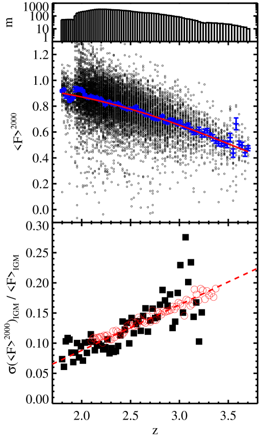
Figure 3.— (upper two panels): Each circle in the middle panel shows a single flux measurement in a 2000  km s^-1 window at the given redshift, with the number of unique measurements $m$ described by the histogram in the top panel. The blue points indicate the average of the $\langle F\rangle^{2000}$ measurements and the standard deviation of the mean. The solid red line shows the mean flux (Equation 2), which was used to modulate the MFR continua of our quasar spectra ($\S$ 2.3.1). There is excellent agreement at all redshifts except at $z\approx 2$ which may be attributed to the poorer data quality of BOSS spectra at $\lambda<3700$Å and to greater uncertainty in our approach to mean flux regulate these data (see also Lee et al., 2013). (lower panel): Black squares show the scatter in the measured $\langle F\rangle^{2000}$ values from the QPQ b/g quasar sightlines, restricted to ${\rm S/N}_{\rm Ly\alpha}>15$ and normalized by the mean flux of the IGM. Given the high signal-to-noise ratio, the variance is dominated by intrinsic fluctuations in the IGM. The red dashed line shows an unweighted, least-squares fit to the values at $z<3$. We recover $\sigma(\langle F\rangle^{2000})_{\rm IGM}/\langle F\rangle_{\rm IGM}=-0.068+0.077z$. For comparison, we present measurements of the scatter from the BOSS sample of Lee et al. (2013, red circles), using the sample of 1927 quasars with S/N $>8$ per pixel. There is excellent agreement between these measurements and our analysis of the QPQ6 dataset.

Table 4QPQ6 H I Measurements

f/g Quasar	b/g Quasar	$R_{\perp}$	Spec.	$z_{\rm fg}$	S/Na	$\langle F\rangle^{2000}$	$\delta_{\langle F\rangle}^{2000}$	$\delta v^{b}$	$\lambda^{c}$	$W_{\rm Ly\alpha}$d	log $N_{\rm HI}$	flg${}_{\rm OT}^{e}$
		(kpc)						(  km s-1)	(Å)	(Å)
J000211.76$-05$2908.4	J000216.66$-05$3007.6	768	SDSS	2.819	41	$0.66$	$0.06$	$-232$	[4633.4,4647.2]	$1.28\pm 0.05$	$<18.00$	0
J000426.43$+00$5703.5	J000432.76$+00$5612.5	882	BOSS	2.812	17	$0.58$	$0.18$	$-429$	[4622.4,4632.6]	$1.33\pm 0.11$		0
J000536.29$+00$0922.7	J000531.32$+00$0838.9	725	BOSS	2.522	10	$0.79$	$-0.02$	$317$	[4279.9,4293.7]	$1.58\pm 0.19$	$<19.00$	0
J000553.32$-03$1200.3	J000551.25$-03$1104.7	533	BOSS	2.547	6	$0.78$	$-0.02$
J000629.92$-00$1559.1	J000633.35$-00$1453.3	711	BOSS	2.333	11	$0.79$	$0.03$	$40$	[4044.8,4060.6]	$1.63\pm 0.21$	$<19.00$	0
J000839.31$-00$5336.7	J000838.30$-00$5156.7	841	BOSS	2.627	23	$0.59$	$0.22$	$551$	[4411.4,4423.2]	$1.55\pm 0.08$	$<18.80$	0
J001028.78$-00$5155.7	J001025.73$-00$5155.3	387	BOSS	2.427	14	$0.68$	$0.15$	$-797$	[4149.4,4159.8]	$1.40\pm 0.11$		0
J001247.12$+00$1239.4	J001250.49$+00$1204.0	532	BOSS	2.157	9	$0.40$	$0.53$
J001351.21$+01$2717.9	J001357.14$+01$2739.2	784	BOSS	2.228	7	$0.79$	$0.05$
J001605.88$+00$5654.2	J001607.27$+00$5653.0	176	BOSS	2.402	7	$0.74$	$0.07$

Note. — [The complete version of this table is in the electronic edition of the Journal. The printed edition contains only a sample.]

We may also compute the variance in a set of $m$ measurements of $\langle F\rangle^{2000}$:

$$\sigma^{2}(\langle F\rangle^{2000})\equiv\frac{\sum\limits_{i=1}^{m}\left(\,\langle F\rangle^{2000}-\overline{\langle F\rangle}\,\right)^{2}}{m}\;\;.$$ (3)

As described above, the variance includes contributions from Poisson noise, continuum placement, and intrinsic variations in the IGM. To isolate the latter effect in the following, we restrict the evaluation to spectra with $S/N>15$ per rest-frame Å at $z_{\rm Ly\alpha}$. The results for the QPQ6 data are shown in Figure 3b, using the same set of redshifts as the upper panel but ending at $z=3.25$ where the sample size is too small. In each case, we have normalized $\sigma(\langle F\rangle^{2000})$ by the mean-flux at each redshift $\langle F\rangle_{\rm IGM}$. We observe a roughly linear increase in $\sigma(\langle F\rangle^{2000})/\langle F\rangle_{\rm IGM}$ with increasing redshift owing to the evolving relationship between transmission in the Ly$\alpha$ forest and overdensity as the universe expands (Hui, 1999). The figure also shows a linear, least-squares fit to the measurements at $z<3$ which yields: $\sigma(\langle F\rangle^{2000})/\langle F\rangle_{\rm IGM}=-0.068+0.077z$. Overplotted on the figure are also a series of $\sigma(\langle F\rangle^{2000})/\langle F\rangle_{\rm IGM}$ measurements drawn from the BOSS dataset of Lee et al. (2013). We find excellent agreement and conclude that our linear fit is a good description for $z<3$. It will be compared, in the following sub-section, against the scatter in $\langle F\rangle^{2000}$ observed in the spectral regions associated with the f/g quasars.

Lastly, we introduce a third statistic which compares a $\langle F\rangle^{\Delta v}$ measurement against the average value at that redshift:

$$\delta_{\langle F\rangle}\equiv\frac{\langle F\rangle_{\rm IGM}-\langle F\rangle^{\Delta v}}{\langle F\rangle_{\rm IGM}}\;\;.$$ (4)

This quantity is analogous to the standard definition of overdensity and is defined to be positive in higher opacity (lower flux) regions. Although it is a relative quantity, it may offer greater physical significance than the values of $\langle F\rangle^{\Delta v}$. Furthermore, by normalizing to $\langle F\rangle_{\rm IGM}$ we may compare measurements from sub-samples of QPQ6 having a range of redshifts.

3.2. H I Measurements at $\lambda_{\rm Ly\alpha}^{\rm fg}$

Consider first the average flux in total intervals $\Delta v=1000,2000$ and $3000\,{\rm km~{}s^{-1}}$ that we refer to as $\langle F\rangle^{1000}$, $\langle F\rangle^{2000}$, and $\langle F\rangle^{3000}$. The largest interval was chosen to have a high probability ($>90\%$) for containing $\lambda_{\rm Ly\alpha}^{\rm fg}$ of the f/g quasar, but it suffers the greatest dilution from unrelated IGM absorption. The smallest velocity window, meanwhile, does not cover even the $\pm 1\sigma_{z}$ uncertainty interval of $z_{\rm fg}$ for many of the f/g quasars. We may also report these measurements in terms of the equivalent width, e.g. $W_{\rm Ly\alpha}^{1000}=(1-\langle F\rangle^{1000})\Delta\lambda^{1000}$ where $\Delta\lambda^{1000}=1215.6701{\rm\AA}\,(1000\,{\rm km~{}s^{-1}})/c$. Table 4 lists the $\langle F\rangle^{\Delta v}$ and $W_{\rm Ly\alpha}$ values measured in these various windows around each f/g quasar. The errors listed refer to statistical errors but the uncertainties are generally dominated by continuum placement. The latter error is systematic and scales roughly as the size of the velocity interval; a $10\%$ error in the normalization translates to $\sigma(W_{\rm Ly\alpha})\approx 0.4$Å for $\Delta v=1000{\rm km~{}s^{-1}}$. This is approximately five times smaller than the average value observed, but it certainly contributes to the scatter in the observed distribution. For ${\rm S/N}_{\rm Ly\alpha}$=10, the statistical error in a 1000  km s^-1 window is $\approx 5-10\%$ depending on the actual $\langle F\rangle^{1000}$ value.

Table 5QPQ6 $\langle F\rangle^{\Delta v}$  Statistics

Sample	$m_{\rm pair}$	$\langle z_{\rm fg}\rangle$	Median	Mean	RMS	IGMa
Full QPQ6 with varying velocity window
1000 km s-1	646	2.415	0.72	0.70	0.21	$0.81$
2000 km s-1	646	2.415	0.73	0.71	0.18	$0.81$
3000 km s-1	646	2.415	0.74	0.73	0.16	$0.80$
Variations with $R_{\perp}$ for a $\Delta v=2000{\rm km~{}s^{-1}}$ window
(0,100) kpc	20	2.045	0.69	0.61	0.22	$0.78$
(100,200) kpc	36	2.137	0.73	0.66	0.22	$0.80$
(200,300) kpc	22	2.376	0.72	0.72	0.17	$0.79$
(300,500) kpc	70	2.333	0.76	0.74	0.19	$0.81$
(500,1000) kpc	451	2.375	0.74	0.73	0.15	$0.82$
(0,300) kpc	78	2.181	0.71	0.67	0.21	$0.81$
(300,1000) kpc	521	2.369	0.75	0.73	0.16	$0.82$

Table 5 provides statistics for these $\langle F\rangle^{\Delta v}$ values for the full QPQ6 sample. In every interval, we find relatively strong absorption at Ly$\alpha$ ($\langle F\rangle^{\Delta v}\,\approx 0.7$). There is also significant dispersion, which decreases with increasing velocity interval. A portion of the scatter is related to continuum placement and fluctuations in the background IGM. Nevertheless, a visual inspection of the spectra reveals many examples with very weak/strong absorption which also implies significant scatter within the quasar environment.

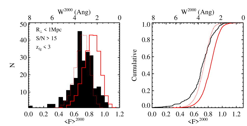
Figure 4.— (left): Histograms of measured $\langle F\rangle^{2000}$ values for the QPQ6 sample restricted to ${\rm S/N}_{\rm Ly\alpha}>15$ and $z_{\rm fg}<3$ (black, filled), the random control sample with identical restrictions (gray, solid line), and the control sample with each $\langle F\rangle^{\Delta v}$ value scaled by the ratio of the means $(1.13)^{-1}$ (gray, dotted). (right): The cumulative $\langle F\rangle^{2000}$ distributions for the three samples shown in the left-hand panel. Even when one scales the control sample to have identical mean as the QPQ6 sample it is a poor description of the data because the latter exhibits much greater scatter. This scatter must be intrinsic to the quasar environment.

A proper assessment of the $\langle F\rangle^{\Delta v}$ values requires placing them in the context of random regions in the Universe (i.e. Figure 3). Scientifically, we aim to establish whether the quasar environment has enhanced or reduced H I absorption relative to such random regions. For each f/g quasar, we randomly chose 10 other quasar pairs from the QPQ6 sample such that the spectral region at $\lambda_{\rm Ly\alpha}^{\rm fg}$: (i) lies within the Ly$\alpha$ forest of the b/g quasar; (ii) lies 1500  km s^-1 redward of Ly$\beta$; (iii) has a velocity separation of at least 3000   km s^-1 from the f/g quasar in that pair; and (iv) lies at least 4000   km s^-1 blueward of the b/g quasar (to avoid its proximity zone). We then measure $\langle F\rangle^{\Delta v}$ and record the values. We achieved 10 matches for all quasars in the sample except for the 9 pairs with $z_{\rm fg}>3.5$. Statistics on the $\langle F\rangle^{\Delta v}$ values for this control sample are also given in Table 5. The quasar pair distributions have lower $\langle F\rangle^{\Delta v}$ values at high statistical significance, e.g. the mean $\langle F\rangle^{2000}$ for the full QPQ6 dataset is 0.71 with an error of 0.007 whereas the control sample has a mean of 0.81 with similar uncertainty. Similarly, a two-sided Kolmogorov-Smirnov (KS) test rules out the null hypothesis of the QPQ6 and control samples being drawn from the same parent population at $>99.99\%$ for any of these velocity intervals.

For the remainder of analysis that follows we focus on measurements in the 2000   km s^-1 window $\langle F\rangle^{2000}$, which we consider to offer the best compromise between maximizing signal from the quasar environment while minimizing IGM dilution. This choice is further motivated by our analysis of individual absorbers ($\S$ 4) and composite spectra ($\S$ 5). Qualitatively, we recover similar results when using other velocity windows.

Figure 4 shows a comparison of $\langle F\rangle^{2000}$ values for a restricted subset of the QPQ6 sample: spectra with ${\rm S/N}_{\rm Ly\alpha}>15$, and $z_{\rm fg}<3$. We restrict to higher S/N in part to examine the intrinsic variance of the distribution by minimizing the contribution of Poisson fluctuations and continuum uncertainty. As with the full QPQ6 distribution, the offset in $\langle F\rangle^{\Delta v}$ values between the pair sample and control distribution is obvious and the KS test rules out the null hypothesis at $>99.99\%$ confidence. We may also compare the dispersion in the $\langle F\rangle^{\Delta v}$ measurements. We measure $\sigma(\langle F\rangle^{2000})=0.17$ for the 245 pairs in this restricted QPQ6 sample. Evaluating our fit to the variance of the IGM $\sigma(\langle F\rangle^{2000})$ ($\S$ 3.1, Figure 3b) at each of the $z_{\rm fg}$ values and averaging the different redshifts, we recover 0.087. An $F$-test yields a negligible probability that the $\langle F\rangle^{2000}$ values from the QPQ6 and control samples have comparable variance. This result is further illustrated in Figure 4 where we compare $\langle F\rangle^{\Delta v}$ distributions of the quasar pairs and the control sample. The dotted line shows the control values scaled by the ratio of the means of the distributions (0.85). This scaled distribution is considerably more narrow than the QPQ6 sample.

The analysis presented above include pairs with a wide distribution of proper separation and a range in redshifts and quasar luminosities (Figure 1). We now consider the influence of several of these factors on the H I absorption strength. We begin with impact parameter $R_{\perp}$, for which we may expect the strongest dependence. We first restrict the QPQ6 sample to pairs with $z_{\rm fg}<3$ to produce a sub-sample of pairs where $z_{\rm fg}$ is less correlated with $R_{\perp}$. Our cut also mitigates against the likelihood that the properties of the halos hosting quasars evolve significantly with redshift, as suggested by clustering analysis (Shen et al., 2007). For example, if higher redshift quasars occur in more massive halos, they might have systematically distinct associated H I absorption. We caution, however, that the pairs with smallest $R_{\perp}$ do have redshifts that are a few tenths smaller than those at larger impact parameter. To further mitigate the effects of IGM evolution, we focus on the $\delta_{\langle F\rangle}$ statistic instead of $\langle F\rangle^{\Delta v}$.

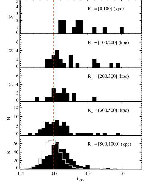
Figure 5.— These panels present the $\delta_{\langle F\rangle}$ distributions for the QPQ6 quasar pairs (restricted to $z_{\rm fg}<3$) in a series of impact parameter intervals. It is evident that the distributions are skewed toward positive values for all of the $R_{\perp}$ intervals. We conclude: (1) the quasar environment exhibits enhanced H I absorption at all impact parameters $R_{\perp}<1$ Mpc; (2) the excess increases with decreasing $R_{\perp}$. In the last panel, we show the distribution of $\delta_{\langle F\rangle}$ values for our control sample (gray curve).

Figure 5 compares the distributions of $\delta_{\langle F\rangle}$ values in a series of $R_{\perp}$ intervals. Each subset exhibits a systematic shift towards positive values, and a two-sided KS test comparison of the values with the control sample rules out the null hypothesis that the f/g quasar distribution is drawn from the same parent population as the ambient IGM. We conclude that there is excess H I Ly$\alpha$ absorption at all impact parameters $R_{\perp}<1$ Mpc from the galaxies hosting $z\sim 2.5$ quasars. We also find that the average $\delta_{\langle F\rangle}$ values increase with decreasing $R_{\perp}$ (see Table 6), indicating the excess is physically associated to the f/g quasar. The Spearman and Kendall tests yield correlation coefficients implying a correlation at $\approx 98\%$ confidence. There is a large dispersion at all $R_{\perp}$, related to intrinsic variations in the H I absorption associated with the f/g quasars, continuum error, and fluctuations within the IGM. Comparing the scatter in these measurements against the control sample, we find systematically larger scatter in the quasar pair distributions. Aside from the $R_{\perp}=[200,300]$ kpc interval (which shows systematically lower $\delta_{\langle F\rangle}$ values), the $F$-test reports a negligible probability that the variances are the same.

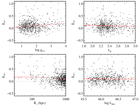
Figure 6.— Scatter plot of $\delta_{\langle F\rangle}$ values versus various observables and physical quantities of the QPQ6 quasar pair sample. For any range of the properties considered, the systematically positive $\delta_{\langle F\rangle}$ values indicate that the quasar pairs exceed that of the control sample, i.e. enhanced H I absorption occurs independently of $g_{\rm UV}$, $z_{\rm fg}$, or quasar luminosity. The only apparent correlation (the red dotted line shows the least-squares, linear fit) is with $\log g_{\rm UV}$ which scales inversely with $R_{\perp}$; therefore, this reflects a result similar to that presented in Figure 5.

In Figure 6, we show a series of scatter plots comparing $\delta_{\langle F\rangle}$ with various observables and physical quantities of the quasar pairs: Bolometric luminosity, $g_{\rm UV}$, $z_{\rm fg}$, and $R_{\perp}$. We find the $\delta_{\langle F\rangle}$ values are systematically positive indicating that the quasar pairs exhibit enhanced H I absorption independently of $g_{\rm UV}$, $z_{\rm fg}$, or quasar luminosity. Furthermore, the only quantity besides $R_{\perp}$ where $\delta_{\langle F\rangle}$ exhibits a correlation is for $g_{\rm UV}$, and we recognize this as an equivalent result because $g_{\rm UV}\propto R^{-2}$.

To briefly summarize (see $\S$ 6 for further discussion), the 1 Mpc environment surrounding quasars exhibit enhanced H I Ly$\alpha$ absorption in their transverse dimension. The excess trends inversely with impact parameter indicating a higher density and/or neutral fraction in gas towards the center of the potential well. The distribution of $\langle F\rangle^{\Delta v}$ and $\delta_{\langle F\rangle}$ values also show a larger scatter than the ambient IGM. The enhanced absorption holds independently of any property of the quasar or pair configuration.

Table 6QPQ6 $\delta_{\langle F\rangle}$  Statistics

Sample	$m_{\rm pair}$	$\langle z_{\rm fg}\rangle$	Median	Mean	RMS
Variations with $R_{\perp}$
(0,100) kpc	12	2.204	0.35	0.38	0.08
(100,200) kpc	23	2.318	0.09	0.22	0.09
(200,300) kpc	18	2.494	0.11	0.11	0.03
(300,500) kpc	63	2.388	0.05	0.08	0.06
(500,1000) kpc	438	2.392	0.07	0.08	0.03
(0,300) kpc	53	2.352	0.15	0.22	0.08
(300,1000) kpc	501	2.391	0.06	0.08	0.04

4. H I Absorption from Individual Systems Associated to the f/g Quasar

In QPQ5 we demonstrated that a high fraction ($\approx 60\%$) of the quasar pair sightlines with $R_{\perp}<200$ kpc intersect optically thick gas surrounding the f/g quasar (see also QPQ1, QPQ2, and QPQ4). Furthermore, the majority of these optically thick systems exhibit strong, metal-line absorption from lower ionization transitions (QPQ5; Farina et al., 2013). Such absorbers occur relatively rarely in b/g quasar sightlines through the intervening IGM (i.e. far from f/g quasars), and are thus qualitatively distinct from the canonical Ly$\alpha$ forest. In this respect, some of the excess absorption revealed by Figure 4 must be related to the individual absorption systems traditionally surveyed by quasar absorption-line researchers, e.g. the Lyman limit systems (LLSs) and damped Ly$\alpha$ systems (DLAs). Motivated by these results, we perform an analysis of the strongest absorption system associated to each f/g quasar in a $\pm 1500{\rm km~{}s^{-1}}$ velocity interval. We adopt a larger velocity window than the fiducial 2000  km s^-1 used for the $\langle F\rangle^{\Delta v}$ measurements in the previous section to increase the confidence that our analysis includes the strongest absorption related to the f/g quasar (i.e. to more conservatively account for error in the f/g quasar redshifts).

At $z>2$, absorption surveys have tended to focus on strong Ly$\alpha$ absorbers (e.g. O’Meara et al., 2007; Prochaska & Wolfe, 2009; Prochaska et al., 2010; Noterdaeme et al., 2012) and/or gas selected by metal-line absorption (e.g. Nestor et al., 2005; Cooksey et al., 2013). The definition of these absorption systems is somewhat arbitrary and are not always physically motivated, e.g. the velocity window chosen for analysis, the equivalent width limit adopted. Similarly, the results derived in the following are not as rigidly defined as those of the preceding section. Nevertheless, there is strong scientific value to this approach and we again derive a control sample to perform a relative comparison to the “ambient” IGM.

4.1. System Definition and Equivalent Widths

We have adopted the following methodology to define and characterize individual absorption systems associated to the f/g quasar. First we searched for the strongest Ly$\alpha$ absorption feature in the $\pm 1500{\rm km~{}s^{-1}}$ velocity interval centered on $\lambda_{\rm Ly\alpha}^{\rm fg}$ for every QPQ6 pair with ${\rm S/N}_{\rm Ly\alpha}>9.5$. This velocity criterion allows for uncertainty in $z_{\rm fg}$ and for peculiar motions within the halos. The ${\rm S/N}_{\rm Ly\alpha}$ criterion was imposed to limit the sample to spectra with better constrained continua and higher quality data for the Ly$\alpha$ line assessment and associated metal-line absorption. A total of 572 pairs were analyzed. Second, we set a velocity region for line-analysis based on the line-profile and the presence of metal-line absorption (rarely detected). The region generally only encompassed the strongest, Gaussian-like feature at Ly$\alpha$ but line-blending did impose a degree of subjectivity. Third, we measured the equivalent width across this region, estimated the H I column density, and assessed the likelihood that the absorption system is optically thick at the Lyman limit. In the Appendix, we show a few examples of this procedure.

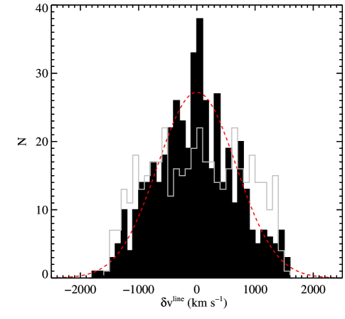
Figure 7.— The solid black histogram presents the velocity offsets $\delta v^{\rm line}$ for the strongest absorption lines in a $\pm 1500{\rm km~{}s^{-1}}$ interval about $\lambda_{\rm Ly\alpha}^{\rm fg}$ of the f/g quasars. The distribution has a Gaussian profile with a mean $<\delta v^{\rm line}>\,=-30{\rm km~{}s^{-1}}$ and a scatter $\sigma(\delta v^{\rm line})=670{\rm km~{}s^{-1}}$, as traced by the dashed red line. This distribution is consistent with the estimated error in our $z_{\rm fg}$ measurements. The gray histogram shows the $\delta v^{\rm line}$ distribution for a control sample. It is nearly uniform across the $\pm 1500{\rm km~{}s^{-1}}$ interval.

To explore systematic effects associated with the ‘by-eye’ line identification, we repeated this analysis for a random control sample of 572 sightlines matched to our pair samples. Specifically, this control sample assumes the same $z_{\rm fg}$ distribution of the QPQ6 subset but we analyze the spectral region in the Ly$\alpha$ forest of a randomly chosen spectrum taken from the full set of b/g quasar data but restricted the b/g quasar as follows: we demanded that the spectral region covering $\lambda_{\rm Ly\alpha}^{\rm fg}$ lies redward of the Ly$\beta$ emission line, away from the Ly$\alpha$ emission line, and away from the known f/g quasar associated to the b/g spectrum. Figure 7 presents the velocity offsets $\delta v^{\rm line}$ between the line centroid and $\lambda_{\rm Ly\alpha}^{\rm fg}$ for each of the QPQ6 pairs. These are centered near zero, have a Gaussian distribution, and show an RMS of 670  km s^-1 that is consistent with the redshift uncertainties of the f/g quasars. The figure also shows the $\delta v^{\rm line}$ distribution for the control sample. It is nearly uniform, as expected for a random sample. We have also examined the velocity offset as a function of impact parameter. The scatter is smaller for $R_{\perp}<300$ kpc, suggesting a more physical association between the gas and f/g quasar. It may also reflect, however, a somewhat smaller uncertainty in $z_{\rm fg}$ for that subsample.

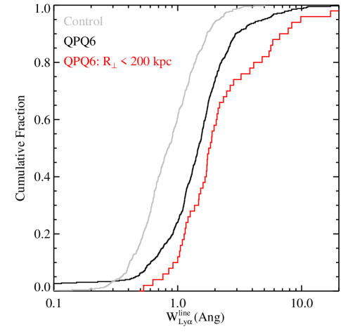
Figure 8.— The black curve traces the cumulative distribution of the rest-frame equivalent widths for the strongest absorption line system in a $\pm 1500{\rm km~{}s^{-1}}$ interval around $\lambda_{\rm Ly\alpha}^{\rm fg}$ of the f/g quasars from QPQ6. The gray curve is the cumulative distribution for a control sample. It shows systematically lower $W_{\rm Ly\alpha}^{\rm line}$ values. The red histogram traces the cumulative distribution from the subset of quasar pairs with $R_{\perp}<200$ kpc. These pairs show systematically larger $W_{\rm Ly\alpha}^{\rm line}$ values and a two-sided KS test rules out the null hypothesis that these are drawn from the same parent sample at high confidence ($P_{\rm KS}=0.005$).

The cumulative distribution of $W_{\rm Ly\alpha}^{\rm line}$ values is presented in Figure 8. We report values ranging from a few 0.1Å to over 10Å, with the majority of the sample having $W_{\rm Ly\alpha}^{\rm line}\approx 1-2$Å. This distribution is compared against the control sample, which shows systematically lower $W_{\rm Ly\alpha}^{\rm line}$ values than the QPQ6 measurements. For example, 60% of the random sample have $W_{\rm Ly\alpha}^{\rm line}<1$Å in comparison to fewer than 25% of the true quasar pairs. We also show the cumulative distribution for the 32 pairs with $R_{\perp}<200$ kpc and find that it is shifted towards even larger $W_{\rm Ly\alpha}^{\rm line}$ values. A two-sided KS test comparing the full distribution (which includes the low $R_{\perp}$ pairs) to the small separation pairs yields a low probability ($P_{\rm KS}=0.02$) that the two distributions are drawn from the same parent population. The probability is even lower if we compare the low $R_{\perp}$ pairs with pairs at $R_{\perp}>500$ kpc ($P_{\rm KS}=0.005$). We conclude at high confidence that the average strength of associated H I absorption lines increase with decreasing $R_{\perp}$.

4.2. $N_{\rm HI}$ Measurements

While $W_{\rm Ly\alpha}^{\rm line}$ is a direct observable that reliably gauges the H I absorption strength, it has limited physical significance. For several scientific pursuits, one would prefer to estimate the total surface density of H I gas, i.e. the H I column density $N_{\rm HI}$. As Figure 8 indicates, however, the majority of absorbers exhibit $W_{\rm Ly\alpha}^{\rm line}\approx 1-2$Å, which places the systems on the flat portion of the curve-of-growth. In these cases, the data have very poor sensitivity to the $N_{\rm HI}$ value; instead $W_{\rm Ly\alpha}^{\rm line}$ primarily traces the kinematics of the system. Nevertheless, one may resolve the damping wings of Ly$\alpha$ for systems with large $N_{\rm HI}$ values ($>10^{19}\,{\rm cm^{-2}}$). There is also a small set of systems showing very weak absorption ($W_{\rm Ly\alpha}^{\rm line}\ll 1$Å) which provide upper limits to $N_{\rm HI}$. As described below, we have also estimated $N_{\rm HI}$ in a broad bin to classify the gas as being optically thick to ionizing radiation (i.e. $N_{\rm HI}\gtrsim 10^{17.3}\,{\rm cm^{-2}}$).

For each system with $W_{\rm Ly\alpha}^{\rm line}>1.4$Å, we have performed a Voigt-profile analysis of the Ly$\alpha$ absorption. When metal-lines are present, we have set the Ly$\alpha$ absorption redshift to correspond to the centroid of these features. We then fit the $N_{\rm HI}$ value of the Ly$\alpha$ line while simultaneously making minor modifications to the local continuum as necessary (e.g. Prochaska et al., 2005; O’Meara et al., 2007). The data and profile fits for all of the systems with measured $N_{\rm HI}\geq 10^{19}\,{\rm cm^{-2}}$ are presented in the Appendix. For those lines without damping wings, we set a conservative upper limit to $N_{\rm HI}$ based on the observed profile. Furthermore, systems with $W_{\rm Ly\alpha}^{\rm line}<1.4$Å are conservatively assigned to have $N_{\rm HI}<10^{18.5}\,{\rm cm^{-2}}$. We also analyzed the $\approx 100$ pairs with ${\rm S/N}_{\rm Ly\alpha}>30$ where one can place much tighter upper limits to $N_{\rm HI}$ when the absorption is very weak. This yielded a set of systems with $N_{\rm HI}<10^{17.3}\,{\rm cm^{-2}}$.

The resultant $N_{\rm HI}$ values and upper limits are listed in Table 4. Uncertainties in these measurements are dominated by the systematic errors of continuum placement and line-blending. We estimate $1\sigma$ uncertainties of 0.15 dex for $N_{\rm HI}\geq 10^{20}\,{\rm cm^{-2}}$ where the absorption is strongest and 0.25 dex for systems having $10^{19}\,{\rm cm^{-2}}N_{\rm HI}<10^{20}\,{\rm cm^{-2}}$ where line-blending is a particular concern. We have not attempted to measure $N_{\rm HI}$ values below $10^{19}\,{\rm cm^{-2}}$ but do impose upper limits below this threshold. For systems with $N_{\rm HI}\approx 10^{19}\,{\rm cm^{-2}}$, the error will not be distributed normally; there will be occasional catastrophic failures of erroneously classified high-column density systems, for which the actual value $N_{\rm HI}\ll 10^{19}\,{\rm cm^{-2}}$ due to unidentified blending.

In our first pass, we fitted $\approx 60$ systems with $N_{\rm HI}\geq 10^{19}\,{\rm cm^{-2}}$ and noted that a significant fraction of these have $N_{\rm HI}\approx 10^{19}\,{\rm cm^{-2}}$ which produces a damped Ly$\alpha$ profile that is marginally resolved in our lower resolution data. These same classification criteria resulted in an excess incidence for our random sightlines over the expectation from previous surveys (e.g. O’Meara et al., 2007). Therefore, we reexamined each of these systems (the QPQ6 and random samples) for the presence of associated low-ion absorption (e.g. C II 1334, Al II 1670) and line-blending. To be conservative, we have set all of the systems without low-ion absorption or obvious damping wings to have upper limits to $N_{\rm HI}$. This gave an incidence in the random sample that is lower than expectation (albeit consistent within Poisson uncertainty; 3 observed with 5.5 expected) and reduced the QPQ6 sample of secure $N_{\rm HI}$ measurements. Given the results on the control sample, we expect if anything that these conservative criteria have led us to underestimate the incidence of systems with $10^{19}\,{\rm cm^{-2}}<N_{\rm HI}<10^{20}\,{\rm cm^{2}}$ associated to f/g quasars. We compare the resultant $N_{\rm HI}$ distributions in the Appendix.

We have also examined the data at the Lyman limit for the $\approx 50$ pairs with wavelength coverage. Most of these data are either compromised by Lyman limit absorption from a higher redshift system or poor S/N. For those with good coverage, the presence/absence of strong Lyman limit absorption is consistent with the $N_{\rm HI}$ values estimated from Ly$\alpha$.

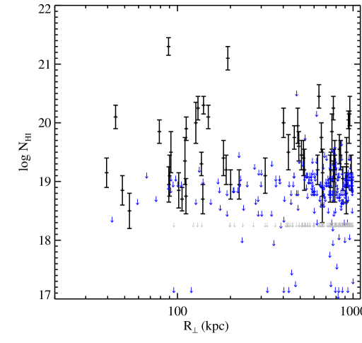
Figure 9.— Scatter plot of the estimated $N_{\rm HI}$ measurements and upper limits against impact parameter for the QPQ6 dataset (restricted to ${\rm S/N}_{\rm Ly\alpha}>9.5$). Perhaps the only discernable trend is a higher incidence of measured values at low $R_{\perp}$ indicating higher $N_{\rm HI}$ values for sightlines penetrating the putative CGM of the quasar environment (see also QPQ5). The gray arrows refer to the 134 cases with $W_{\rm Ly\alpha}^{\rm line}<1.4$Å and ${\rm S/N}_{\rm Ly\alpha}<30$ where we have automatically assigned an upper limit to $N_{\rm HI}$ of $10^{18.3}\,{\rm cm^{-2}}$.

Figure 9 presents a plot of the $N_{\rm HI}$ values against impact parameter. The result is a complicated scatter plot dominated by upper limits. It is somewhat evident, however, that the pairs with $R_{\perp}<200$ kpc have a much higher incidence of measured $N_{\rm HI}$ values than the pairs at larger impact parameters. Furthermore, the measured values at all $R_{\perp}$ are dominated by systems with $N_{\rm HI}\approx 10^{19}\,{\rm cm^{-2}}$ and there are very few systems satisfying the damped Ly$\alpha$ (DLA) criterion, $N_{\rm HI}^{\rm DLA}\geq 2{\;\times\;10^{20}}\,{\rm cm^{-2}}$ (Wolfe et al., 2005). In $\S$ 6, we analyze these measurements to study the clustering and covering fractions of strong H I absorbers in the extended, transverse environment of luminous quasars.

Given the equivalent width for Ly$\alpha$ absorption, our Voigt profile fits for the $N_{\rm HI}$, the presence/absence of Lyman limit absorption, and the presence/absence of low-ion metal absorption, objects were classified into three categories: optically thick, ambiguous, or optically thin. Objects which show obvious damping wings, Lyman limit absorption, or strong ($W>0.3$ Å) low-ion metal absorption are classified as optically thick. For the metals, we focused on the strongest low-ion transitions commonly observed in DLAs (e.g. Prochaska et al., 2001): Si II $\lambda 1260,1304,1526$, O I $\lambda 1302$, C II $\lambda 1334$ Mg II $\lambda 2796,2803$. A complete description of the metal-line analysis will be presented in QPQ7 (Prochaska et al., in prep.). For those cases where metal-lines are weak, are not covered by our spectral coverage, or are significantly blended with the Ly$\alpha$ forest of the b/g quasar, a system is classified as optically thick only if it has $W_{\rm Ly\alpha}\geq 1.8$ Å in a single, Gaussian-like line. For a single line with Doppler parameter $b=40{\rm km~{}s^{-1}}$, this equivalent width threshold corresponds to $N_{\rm HI}>10^{18.5}\,{\rm cm^{-2}}$. There may be a significant number of cases, however, where unresolved line-blending yields such a high equivalent width in a system with a total $N_{\rm HI}<10^{18}\,{\rm cm^{-2}}$. When in doubt, we designated the systems as ambiguous. Note that this evaluation differs slightly from our previous efforts (QPQ1,QPQ2,QPQ4,QPQ5) and the classifications are not identical but very similar.

The completeness and false positive rate of this analysis are sources of concern. Line-blending, in particular, can significantly bias $W_{\rm Ly\alpha}$ and the column density high. We have assessed this estimate with our control sample, having evaluated each random sightline for the presence of optically thick gas. We detect $\approx 25\%$ more LLS (defined to be systems with $N_{\rm HI}>10^{17.3}\,{\rm cm^{-2}}$) in the control sample than expectation from previous surveys (Prochaska et al., 2010; O’Meara et al., 2013). The results are within the Poisson uncertainty (19 detected to 14.7 expected) but we allow that the QPQ6 sample may contain a modest set of false positives. We stress, however, that a majority of these systems in the pair sample also exhibit strong low-ion metal absorption (e.g. C II 1334; QPQ5).

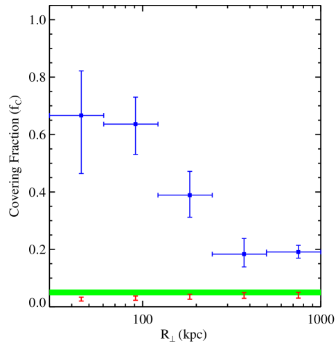
Figure 10.— Estimates for the covering fraction $f_{C}$ of optically thick absorbers for the QPQ6 sample in logarithmic bins of impact parameter. These are presented formally as lower limits owing to the preponderance of ambiguous cases. The red symbols trace the expectation for random quasar sightlines for a $\pm 1500{\rm km~{}s^{-1}}$ interval, estimated at $z_{\rm fg}$ and using $\ell(X)$ from Ribaudo et al. (2011). The green band shows the measured incidence in our control sample which is in good agreement but $\approx 25\%$ above random expectation.

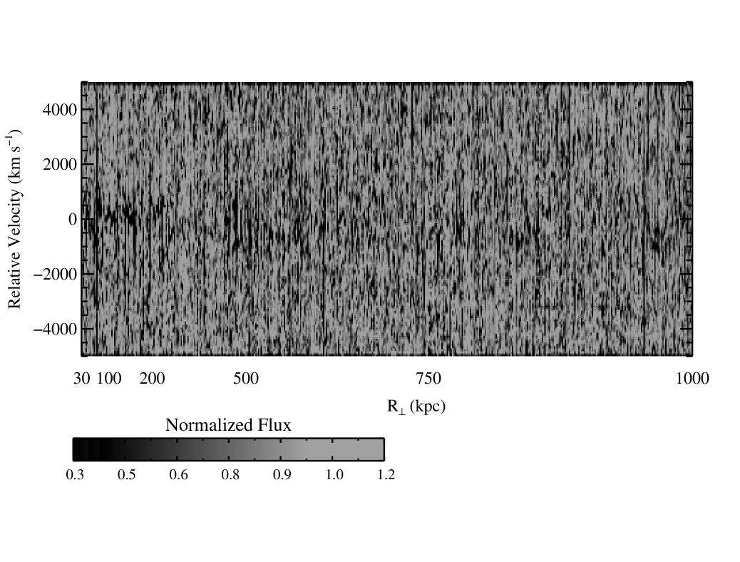
Figure 11.— Map of the normalized flux, spectrum-by-spectrum ordered by impact parameter $R_{\perp}$, around Ly$\alpha$ of the f/g quasars for the QPQ6 sample (restricted to pairs with ${\rm S/N}_{\rm Ly\alpha}>8$ and $z_{\rm fg}<3$). Each spectrum has been linearly interpolated onto a fixed velocity grid with 100  km s^-1 pixels, preserving equivalent width. One notes a likely enhancement in H I absorption at $\delta v=0{\rm km~{}s^{-1}}$ for nearly all impact parameters. The few cases which appear as nearly a single, black line correspond to DLAs.

Figure 10 presents the covering fraction $f_{C}$ of optically thick gas in logarithmic bins of $R_{\perp}$. As discussed in our previous work (QPQ1, QPQ2, QPQ4, QPQ5), $f_{C}$ exceeds 50% for $R_{\perp}<200$ kpc, a remarkable result which reveals a massive, cool CGM surrounding $z\sim 2$ quasars. With the QPQ6 sample, we extend the $f_{C}$ measurements to 1 Mpc (Table 7). We find that $f_{C}$ declines with increasing $R_{\perp}$, with a marked decline at $\approx 200$ kpc which we have interpreted as the ‘edge’ of the CGM (QPQ5). For a halo of mass $M\approx 10^{12.5}{\rm\ M}_{\odot}$ at $z=2.5$, this modestly exceeds the the virial radius ($r_{\rm vir}\approx 160$ kpc). Nevertheless, the covering fraction remains significant ($f_{C}=19\pm 2\%$) for $R_{\perp}>500$ kpc.

Table 7QPQ6 $f_{C}$ Values

$R_{\perp}^{\rm min}$	$R_{\perp}^{\rm max}$	$m_{\rm pair}$	$f_{C}$	$+1\sigma^{a}$	$-1\sigma^{a}$	$f_{C}^{\rm IGM}$
(kpc)	(kpc)
30	60	6	0.67	0.16	0.20	0.03
60	122	22	0.64	0.09	0.11	0.03
122	246	36	0.39	0.08	0.08	0.03
246	496	60	0.18	0.05	0.04	0.04
496	1000	304	0.19	0.02	0.02	0.04

The red points in Figure 10 show estimates for $f_{C}^{\rm IGM}$ for the IGM in a random $\pm 1500{\rm km~{}s^{-1}}$ interval evaluated at $<z_{\rm fg}>$ using the $\ell(X)$ measurements of O’Meara et al. (2013). These may be compared against the $f_{C}$ value measured from our control sample (green band). The two are in fair agreement although, as noted above, we modestly overpredict the incidence in the control sample. Nevertheless, even for $R_{\perp}=[496,1000]$ kpc we find the $f_{C}$ value for the QPQ6 pairs exceeds random by nearly a factor of 5. We conclude that the excess H I absorption inferred from our statistical measures (e.g. Figure 5), is also manifest in the strong Ly$\alpha$ systems which are generally attributed to the ISM and CGM of individual galaxies (Fumagalli et al., 2011b; van de Voort & Schaye, 2012). Furthermore, there is an enhancement at all scales $R_{\perp}\leq 1$ Mpc. We further develop and explore the implications of these results in $\S$ 6.

5. Stacked Spectrum Analysis

The previous sections demonstrated that the environment surrounding $z\sim 2$ quasars (from $R_{\perp}=30$ kpc to 1 Mpc) exhibits excess H I Ly$\alpha$ absorption relative to random spectral regions of normalized quasar spectra. We have reached this conclusion through a statistical comparison of the distribution of $\langle F\rangle^{\Delta v}$ and $\delta_{\langle F\rangle}$ values and equivalent widths measured about each f/g quasar compared to the distribution of a control sample for the IGM ($\S$ 3.2, Figure 4; $\S$ 4.1, Figure 8). We reached a similar conclusion from the incidence of optically thick absorption and the observed distributions of $N_{\rm HI}$ values ($\S$ 4.2, Figure 9,10). We also presented evidence that the excess H I absorption decreases with increasing impact parameter (Figure 5) albeit with substantial scatter from sightline to sightline. This scatter in the absorption strength (e.g. $\langle F\rangle^{\Delta v}$) is driven by continuum error, intrinsic scatter in quasar environments, redshift error for the f/g quasar, and the stochastic nature of the IGM.

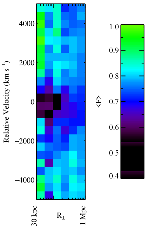
Figure 12.— A map of the normalized flux around Ly$\alpha$ of the f/g quasars in QPQ6 as presented in Figure 11 but rebinned onto 6 logarithmic $R_{\perp}$ intervals spanning from 30 kpc to 1 Mpc and in velocity channels of 400  km s^-1. One observes a clear enhancement in absorption at $\delta v\approx 0{\rm km~{}s^{-1}}$ which decreases with increasing $R_{\perp}$ and velocity offset. Note that the first column corresponds to only 6 quasar pairs and is dominated by sample variance.

There is a complementary approach to assessing the excess (or deficit) of H I Ly$\alpha$ absorption which averages over several of these sources of uncertainty: the creation of composite spectra. A composite spectrum is made by first shifting the individual spectra to the rest-frame of the f/g quasar at Ly$\alpha$ ($\delta v=0{\rm km~{}s^{-1}}$ corresponds to $\lambda_{\rm Ly\alpha}^{\rm fg}$). One then combines them with a statistical measure (e.g. average, median) in fixed velocity intervals, weighting the individual spectra as desired. There are several benefits to this approach. In particular, one averages down the stochasticity of the IGM to (ideally) recover a nearly uniform absorption level in the absence of any other signals. Errors in continuum placement are also averaged down and primarily affect the precision with which one measures the IGM opacity. Therefore, one may then search for excess (deficit) absorption at $\delta v\approx 0{\rm km~{}s^{-1}}$ relative to the IGM level. This provides a robust consistency check on results from the previous sections. Quasar redshift error, Hubble flow, and peculiar motions spread out the absorption, but the total equivalent width can be preserved by using a straight average. This technique also generates spectra as a function of velocity relative to $z_{\rm fg}$. We expect the measured velocity spreads to be dominated by quasar redshift uncertainty, but one can also constrain other processes that generate motions of the gas.

This technique was successfully applied in QPQ5 to assess the average H I absorption strength in that sample, i.e. on scales $R_{\perp}\leq 300$ kpc. We observed strong, excess absorption which we concluded traces the CGM of galaxies hosting $z\sim 2$ galaxies. In this section, we extend the analysis to 1 Mpc and perform an assessment of the technique and its uncertainties. In all of the following, we restrict to the subset of the QPQ6 sample with ${\rm S/N}_{\rm Ly\alpha}>8$ and $z_{\rm fg}<3$. These criteria provide a more uniform set of high-quality input spectra.

Before proceeding to generate composite spectra, it is illustrative to first examine maps of the normalized flux. Figure 11 presents the $\pm 5000{\rm km~{}s^{-1}}$ interval surrounding each f/g quasar, ordered by impact parameter and restricted to the QPQ6 sample with ${\rm S/N}_{\rm Ly\alpha}>8$ and $z_{\rm fg}<3$. Each spectrum has been linearly interpolated (conserving equivalent width), onto a fixed velocity grid centered at $\lambda_{\rm Ly\alpha}^{\rm fg}$ with bins of 100  km s^-1. For velocity bins of this size, we found it unnecessary to smooth the data to a common spectral resolution. A visual inspection reveals obvious excess H I Ly$\alpha$ absorption at $\delta v=0{\rm km~{}s^{-1}}$ from $R_{\perp}=30$ kpc to $R_{\perp}=500$ kpc and likely beyond. The absorption scatters about $\delta v=0{\rm km~{}s^{-1}}$ by many hundreds   km s^-1 and an impression is given that the absorption declines with increasing $R_{\perp}$.

Figure 12 presents a rebinned image, generated by combining the sightlines in 6 logarithmic intervals in $R_{\perp}$, from 30 kpc to 1 Mpc and sampling in velocity space with 400  km s^-1 bins. We have stretched this image to accentuate the excess absorption and to illustrate the decreasing absorption strength with increasing $R_{\perp}$. We caution that the first column reflects only 6 pairs and is dominated by sample variance (the second column corresponds to 14 pairs). Nevertheless, this image illustrates the primary result of this manuscript: the quasar environment is characterized by an excess of H I absorption to 1 Mpc with a decreasing enhancement with $R_{\perp}$ and $|\delta v|$.

In principle, one could fit a global model to the full dataset presented in Figure 11 to estimate the average H I absorption as a function of $R_{\perp}$ (or any other quantity). This might maximize the statistical power of QPQ6 but would require a comprehensive model of the IGM, a proper treatment of the diversity in spectral resolution, and complex models for the CGM surrounding these massive galaxies. We defer such model comparisons to our study of the transverse proximity effect (TPE), using these data and additional pairs with larger separations. Here, we instead explore the nature of excess H I absorption through the generation of composite spectra.

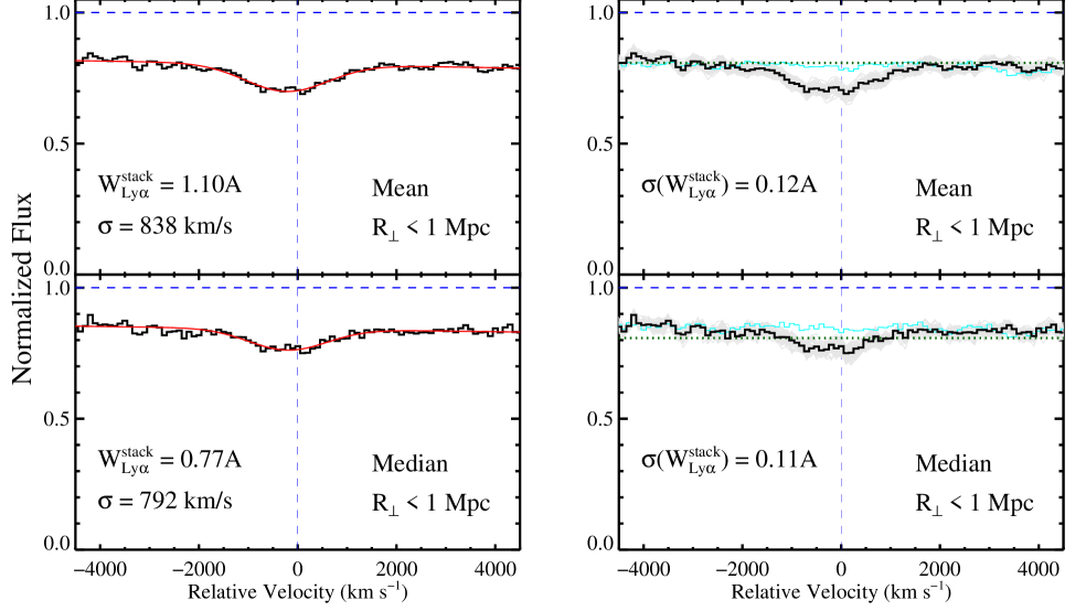
Figure 13.— Mean and median absorption at Ly$\alpha$ of the f/g quasars for all QPQ6 pairs with ${\rm S/N}_{\rm Ly\alpha}>8$ and $z_{\rm fg}<3$. The median impact parameter is at $R_{\perp}=702$ kpc. The left-hand panels show the composites (black) for the mean (upper) and median (lower) statistics. Overplotted on each these is a Gaussian fit (red), normalized to a pseudo-continuum given by the average IGM opacity away from $\delta v=0{\rm km~{}s^{-1}}$. The right-hand panels show the same composites and also a series of bootstrap realizations (gray). In addition, a composite spectrum generated from a control sample of sightlines is presented (cyan). It shows essentially constant IGM opacity at all $\delta v$ (i.e. no excess H I absorption) which matches the opacity used to mean-flux regulate the continua (green dotted line; $\S$ 2.3.1, Equation 2).

We generate composite spectra by simply combining the individual spectra shown in Figure 11. The results one obtains are somewhat sensitive to the specific methodology used to generate the composite spectra. We have experimented with various approaches and adopt the following. First, a minimum of 20 individual spectra are required to sufficiently reduce the stochasticity of the IGM and thereby yield a robust estimate of the average opacity at $|\delta v|\gg 0{\rm km~{}s^{-1}}$. Second, we found that imposing a ${\rm S/N}_{\rm Ly\alpha}$ threshold of 8 on the individual spectra offers a good compromise between maximizing sample size while reducing the likelihood of severe continuum error and/or Poisson noise. Regarding the statistic to generate the composite (e.g. average, median) and how to weight the data (e.g. ${\rm S/N}_{\rm Ly\alpha}$, f/g quasar luminosity), we consider a few scientifically motivated approaches.

Our primary scientific interest is to measure the excess/decrement of H I Ly$\alpha$ absorption associated with the CGM and extended environment of the massive galaxies hosting $z\sim 2$ quasars. Each quasar pair gives an independent probe of this region, i.e. all pairs have equal weight, at least at a given impact parameter. This suggests the composites should be created without any weighting factor. On the other hand, the b/g quasar luminosity should be independent of the f/g quasar’s gaseous environment and one is tempted to weight the spectra by the measured ${\rm S/N}_{\rm Ly\alpha}$ value. This would increase, however, the measured scatter in the IGM absorption because it effectively reduces the number of sightlines included in the composite. Scatter in the composite spectrum is dominated by randomness in the IGM instead of other error sources (i.e. continuum error and photon statistics). Further, the distribution of ${\rm S/N}_{\rm Ly\alpha}$ is pretty narrowly distributed around 10 for the majority of the pairs, with a long tail to high ${\rm S/N}_{\rm Ly\alpha}$ values (Figure 1). Therefore, we have proceeded using equal weights

Regarding the statistics, an average of the individual spectra yields the best estimate of the mean H I Ly$\alpha$ absorption and should preserve the equivalent width. This statistic, however, is more sensitive to outliers, e.g. the occasional DLA system with $W_{\rm Ly\alpha}>10$Å. The median statistic, in contrast, may provide a better estimate for the ‘typical’ absorption. In the following, we generate composite spectra using each of these statistics.

Figure 13 presents the mean and median composite spectra, generated from the full set of data shown in Figure 11. One observes significant absorption at all velocities on the order of $20-25\%$ ($\tau\approx 0.25$). This absorption is driven by the IGM and the observed decrement agrees with previous estimates at $z\gtrsim 2$, as designed ($\S$ 2.3.1). At $\delta v\approx 0{\rm km~{}s^{-1}}$, one identifies an excess of absorption which we associate to H I gas in the local environments of the f/g quasars. The depression is many hundreds   km s^-1 wide, presumably owing to quasar redshift error, peculiar motions, ’virial motions’ and infall in the QSO environment, and Hubble flow. To perform a quantitative assessment, we have fitted Gaussian profiles to each composite spectrum. The fit is performed relative to a pseudo-continuum defined by the IGM absorbed regions (i.e. at a level near 0.8 in the normalized flux, not unity). This continuum was measured through a least-squares linear fit to each pixel in the composite spectrum with $\delta v<-3000{\rm km~{}s^{-1}}$ or $\delta v>2000{\rm km~{}s^{-1}}$. We estimate a less than $2\%$ normalization error in this evaluation. The Gaussian fits, meanwhile, were limited to the pixels at $|\delta v|\leq 1350{\rm km~{}s^{-1}}$ to minimize the effects of metal-line blending (see below). The width that we recover for the Gaussian ($\sigma=822{\rm km~{}s^{-1}}$) is dominated by redshift error. The reported equivalent widths are relative to the pseudo-continuum and are approximately 1Å in strength. Because these are relative to the mean flux and not the normalized flux of the quasars, they relate much more closely to the $\delta_{\langle F\rangle}$ statistic (Figure 5) and not the $W_{\rm Ly\alpha}^{\rm line}$ values measured for systems associated to each f/g quasar (Figure 8).

Regarding the mean vs. median composities, the latter has smaller equivalent width ($\approx 25\%$), as we expected, although nearly the same velocity width. Nevertheless, the strong signal in the median indicates a majority of the sightlines exhibit excess H I absorption. Because the composite spectra applied equal weighting, the results in Figure 13 are dominated by the hundreds of pairs in QPQ6 with $R_{\perp}>500$ kpc. We may conclude that the quasar environment exhibits excess absorption to at least 1 Mpc separation. In the right-hand panels of Figure 13, we present additional analysis on these composite spectra. The cyan curves show composite spectra generated from random Ly$\alpha$ forest spectra taken from the same parent sample and using the $z_{\rm fg}$ distribution of the QPQ6 sample. Again, we require that the random regions lie within the Ly$\alpha$ forest of the b/g quasar and away from its known f/g quasar pair. The resultant composites show uniform absorption associated to the IGM at all velocities with a magnitude matching the mean flux used in the MFR continua, given by Equation 2. This gives additional confidence that the observed excess in the QPQ6 composites is solely related to absorption by gas in the environment of the quasar. The gray curves show the composite spectra for 100 bootstrap realizations of the QPQ6 dataset allowing for duplications. The RMS scatter is small – a few percent – at all velocities. Fitting a Gaussian to each of these, we recover a scatter in the measured equivalent widths of 0.14Å for the mean and 0.12Å for the median composite.

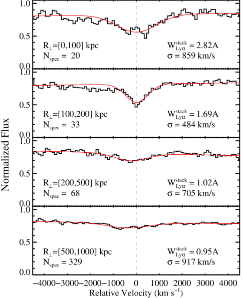
Figure 14.— Mean composites of the QPQ6 sample centered on Ly$\alpha$ of the f/g quasars in increasing, logarithmic intervals of impact parameter $R_{\perp}$. The red curves are Gaussian fits to the composites adopting a continuum fitted to the average opacity (dominated by the IGM) at $|\delta v|\gg 0{\rm km~{}s^{-1}}$. There is excess H I absorption at all impact parameters which decreases with increasing $R_{\perp}$.

Table 8H I Ly$\alpha$ Equivalent Widths from QPQ6 Stacks

$R_{\perp}^{\rm min}$	$R_{\perp}^{\rm max}$	Median $R_{\perp}$	$m_{\rm pair}$	${W_{\rm Ly\alpha}^{\rm stack}}^{a}$	$\sigma(W_{\rm Ly\alpha}^{\rm stack})^{a}$	${W_{\rm Ly\alpha}^{\rm stack}}^{b}$
(kpc)	(kpc)	(kpc)		(Å)	(Å)	(Å)
31	98	89	20	2.82	0.56	2.19
100	199	139	33	1.69	0.50	1.05
201	495	387	68	1.02	0.32	0.53
503	999	786	329	0.95	0.15	0.72

Note. — The mean equivalent width values are well fitted by a power-law, $W_{\rm Ly\alpha}^{\rm stack}(R_{\perp})=2.3$Å($R_{\perp}/100\;\rm kpc)^{-0.46}$.

The maps shown in Figure 11 and 12 indicate a significant trend in absorption strength with $R_{\perp}$. We may study this trend by producing composite spectra in a series of $R_{\perp}$ bins. Figure 14 presents the results for four radial bins, in a series of roughly logarithmic intervals. Similar to the full composites, we detect enhanced absorption at $\delta v\approx 0{\rm km~{}s^{-1}}$ in each of the composites. Additionally, there is an obvious trend of decreasing absorption with increasing $R_{\perp}$. The resultant models are overplotted on the composite spectra (Figure 14) and the fit parameters are listed in Table 8. These single Gaussian models provide a good description of the data, as follows from the central limit theorem. The integrated equivalent widths of these Gaussians clearly decrease with increasing $R_{\perp}$, decreasing from $W_{\rm Ly\alpha}^{\rm stack}=2.8$Å for $R_{\perp}<100$ kpc to $W_{\rm Ly\alpha}^{\rm stack}=1.0$Å for $R_{\perp}>500$ kpc. We note that the values are approximately one half of the average individual $W_{\rm Ly\alpha}^{\rm line}$ values that we measured in $\S$ 4 (Figure 8). We have estimated the error in the equivalent width measurements by bootstrapping each composite 100 times and measuring the RMS in the resultant $W_{\rm Ly\alpha}^{\rm stack}$ values (Table 8). We repeated the analysis on a series of median composite spectra. Similar to the full composites (Figure 13), we detect enhanced absorption at $\delta v\approx 0{\rm km~{}s^{-1}}$ in each of these median composites (Table 8).

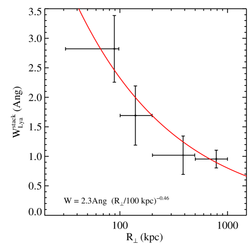
Figure 15.— Equivalent width measurements $W_{\rm Ly\alpha}^{\rm stack}$ for the mean composites in Figure 14. There is a strong, non-linear decline in $W_{\rm Ly\alpha}^{\rm stack}$ with increasing $R_{\perp}$. Each bin is plotted at the median $R_{\perp}$ value of the pairs that contributed to the stack (see Table 8). We have fitted a model of the form $W_{\rm Ly\alpha}^{\rm stack}=W_{0}(R_{\perp}/{\rm 100\,kpc})^{\gamma}$ to the $W_{\rm Ly\alpha}^{\rm stack}$ measurements and their errors (estimated from bootstrap realizations). We find $W_{0}=2.2$Å and $\gamma=-0.45$ and note there is significant degeneracy between the two parameters.

Figure 15 presents the $W_{\rm Ly\alpha}^{\rm stack}$ values for the mean composites versus $R_{\perp}$ for the four intervals, with uncertainties estimated from the bootstrap analysis. There is an obvious, non-linear trend of decreasing $W_{\rm Ly\alpha}^{\rm stack}$ with increasing $R_{\perp}$. We may describe the observed trend with a simple power-law model: $W_{\rm Ly\alpha}^{\rm stack}=W_{0}(R_{\perp}/{\rm 100\,kpc})^{\beta}$. By fitting this two-parameter model to the binned results and assuming Gaussian errors, we find that $\chi^{2}$ is minimized for $W_{0}=2.3$Å and $\beta=-0.46$, with significant degeneracy between the two parameters. We emphasize that this model, despite its relatively good description of the data, is not physically motivated. In fact, we may expect that the observed trend is the result of two competing and (presumably) unrelated physical phenomena (Fumagalli et al., 2013a): the CGM of the host galaxy on scales of $\sim 100$ kpc and clustering of galaxies and other large-scale structures on Mpc scales. It is possible that these combine to give this simple model which describes the observations well.

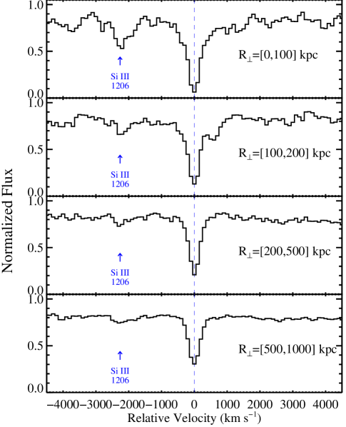
Figure 16.— Mean composites in a series of $R_{\perp}$ intervals using individual spectra shifted to the strongest absorption line in the $\pm 1500{\rm km~{}s^{-1}}$ interval around $z_{\rm fg}$ (see $\S$ 4). At $\delta v\approx-2250{\rm km~{}s^{-1}}$, one identifies significant absorption that we associate with the Si III 1206 transition. Its presence affected how we fit the IGM opacity of our composites and the Gaussian fits to the excess H I absorption. It may also contribute slightly to the estimated $W_{\rm Ly\alpha}^{\rm stack}$ values for the lowest $R_{\perp}$ intervals. Future work will explore the metal-line absorption associated to the quasar environments (QPQ7; see also QPQ3, QPQ5).

There is one, somewhat subtle, feature in the composites for the lowest $R_{\perp}$ intervals: excess absorption at $\delta v\approx-2000{\rm km~{}s^{-1}}$ which gives the impression of greater IGM opacity bluewards of $z_{\rm fg}$. This excess opacity is dominated by Si III 1206 absorption at $z\approx z_{\rm fg}$ which occurs at $\delta v\approx-2250{\rm km~{}s^{-1}}$ bluewards of Ly$\alpha$. Figure 16a shows a series of composite spectra stacked at the flux-weighted centroid of the individual Ly$\alpha$ lines described in $\S$ 4. We recover similar equivalent widths but the Ly$\alpha$ profiles in these composities are, by design, much more narrow than the lines in the composites stacked at $z=z_{\rm fg}$. We also recognize significant excess absorption at $\delta v\approx-2200{\rm km~{}s^{-1}}$ which we associate to Si III 1206 absorption. No other statistically significant absorption is apparent in this velocity interval and none is expected. The presence of strong Si III 1206 absorption, especially for the $R_{\perp}<200$ kpc pairs, motivated our decision to fit the pseudo-continuum of the composite spectra at $\delta v<-3000{\rm km~{}s^{-1}}$. We perform additional analysis on these composites with emphasis on the metal-line absorption in QPQ7. Future work will also re-examine the composite spectra for these quasar pairs when near-IR spectroscopy enables a more precise estimation of $z_{\rm fg}$.

We may explore the dependence of H I absorption on other aspects of the quasars and/or their environment. In Figure 17a we present composite spectra for two sub-samples: (1) pairs with $z_{\rm fg}=[1.6,2.4]$ and an average $<z_{\rm fg}>=2.22$; (2) pairs with $z_{\rm fg}=[2.4,3.5]$ and $<z_{\rm fg}>=2.69$. Each subsample has an average impact parameter $<R_{\perp}>\,\approx 700$ kpc. Both show significant IGM opacity, with a larger value for the higher $z_{\rm fg}$ sample, albeit with modest statistical significance ($\approx 2\sigma$). The results are suggestive that higher $z_{\rm fg}$ quasars exhibit a greater excess of H I absorption, consistent with the picture that these quasars are hosted by more massive halos (Shen et al., 2007).

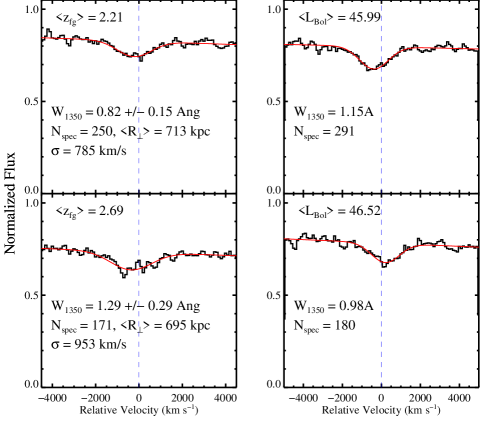
Figure 17.— (left:) Mean composites cut on f/g quasar redshift (at $z_{\rm fg}=2.4$ and restricted to $z_{\rm fg}<3.5$). The two subsamples have very similar $R_{\perp}$ distributions with $\langle R_{\perp}\rangle\approx 700$ kpc. One observes, as expected, that the IGM opacity (evaluated at $\delta v\gg 0{\rm km~{}s^{-1}}$) is higher for the higher $z_{\rm fg}$ subset. We also measure a greater excess of H I absorption at $\delta v\approx 0{\rm km~{}s^{-1}}$, but this is only significant at the $\approx 2\sigma$ level. It is consistent, however, with the expectation that higher redshift quasars are hosted by more massive halos with correspondingly larger H I absorption on these scales. (right:) Mean composites of the QPQ6 sample ($z_{\rm fg}<3$) cut by Bolometric luminosity at $\log L_{\rm Bol}=46.3$. Each subset has a similar mean impact parameter and redshift distribution. Although the two composite spectra have similar equivalent widths, there is an obvious systematic shift in the line centroid of over $500{\rm km~{}s^{-1}}$, which we propose is related to a luminosity-dependent shift in the C IV emission-line of the f/g quasars (i.e. redshift error).

We have also generated composite spectra after splitting the QPQ6 stack-sample by f/g quasar luminosity: $L_{\rm Bol}$ (Figure 17b). There is no statistically significant difference in $W_{\rm Ly\alpha}^{\rm stack}$ for the $L_{\rm Bol}$ subsets, but we do measure a systematic offset in the line-center. We associate this offset with a luminosity-dependent shift in the C IV emission-line (Hewett & Wild, 2010), i.e. error in the f/g redshifts we have measured related to a Baldwin effect. We have generated additional composite spectra cutting on further properties of the sample and find no statistically significant differences. This follows the results of $\S$ 3 where we noted no strong correlation between the mean fluxes and any other property (Figure 6).

6. Analysis and Discussion

In this section we perform additional analysis on measurements from the previous sections and discuss implications for the properties of quasars and the nature of gas in their extended environments.

6.1. Anisotropy in the Quasar Environment

In previous papers in this series, we have concluded that gas observed in absorption in b/g sightlines of quasar pairs is typically not illuminated by the ionizing flux of the f/g quasars. The evidence includes our observation that strong H I absorbers are anisotropically distributed about quasars such that the line-of-sight shows a much lower incidence of strong absorbers than background sightlines (QPQ2), detailed analysis of the observed ionic ratios of heavy elements in a single well-studied quasar absorber do not reflect an intense radiation field (QPQ3), fluorescent Ly$\alpha$ radiation from optically thick gas in the quasar CGM is generally absent (QPQ4), and that there is a high covering fraction of optically thick, cool gas with metals predominantly in low-ionization states (QPQ5). These results are impossible to reconcile with an isotropically emitting source unless quasars vary on very short timescales $\sim 10^{5}$ yr. Furthermore, this anisotropic emission follows naturally from the obscuration frequently invoked in unification models of AGN which center the accreting black hole within an obscuring torus of gas and dust (e.g. Antonucci, 1993; Elvis, 2000; Gaskell, 2009).

The results presented in this manuscript offer further evidence for anisotropic emission. First, we have demonstrated that the environment surrounding $z\sim 2$ quasars exhibits enhanced H I absorption relative to the average IGM (Figure 13). Because the quasar’s ionizing flux exceeds the UV background to 1 Mpc and beyond (Figure 1), one expects a smaller neutral fraction for illuminated gas, and a corresponding decrease H I absorption, absent other effects. Clearly, any reduced absorption caused by ionization effects has been compensated for by the increased absorption caused by the overdensity of gas on scales $R_{\perp}<1$ Mpc. Second, the enhanced H I absorption actually increases with decreasing impact parameter (Figure 5,15), opposite to one’s expectation if ionization effects were playing a dominant role, where the $R^{-2}$ increase in flux would imply a stronger reduction in absorption at smaller impact parameters (see also Font-Ribera et al., 2013). Again, the observed signal implies an increasing density and covering fraction of H I gas towards the quasar. Third, we have established that the high covering fraction of optically thick gas exceeds random expectation even at $R_{\perp}\approx 1$ Mpc (Figure 10).

All of these results run contrary to the characterization of H I Ly$\alpha$ absorption near quasars but along our line-of-sight, where one observes comparable or suppressed absorption relative to the ambient IGM (e.g. Scott et al., 2000; Kirkman & Tytler, 2008; Dall’Aglio et al., 2008) known as the line-of-sight proximity effect (Bajtlik et al., 1988; Scott et al., 2000). We conclude that the environments surrounding $z\sim 2$ are anisotropically illuminated.

This conclusion may be further quantified through a comparison of the clustering signal measured transverse to the quasars with that along the line-of-sight, as estimated from the incidence of proximate absorption systems. Such analysis was first presented in QPQ2. We do not repeat those estimates here, but instead, we consider a different but analogous argument based on covering fractions. We have measured that the covering fraction of optically thick gas at $R_{\perp}<200$ kpc exceeds 50% and that $f_{C}$ increases with decreasing $R_{\perp}$ (Figure 10). Because radiation directed towards us must travel along these scales (and at even smaller separations), we may reasonably assume that $f_{C}$ exceeds 0.5 along the direct line-of-sight i.e. the majority of quasars should exhibit strong Lyman limit absorption near their emission redshifts.

Prochaska et al. (2010) examined the incidence of so-called proximate LLS (PLLS) in their survey of Lyman limit absorption, using $z>3.5$ quasars drawn from the SDSS. They found a modest deficit in the incidence of PLLS (measured within 3000  km s^-1 of $z_{\rm em}$) relative to intervening LLS, discovering only 35 PLLS in over 450 quasars surveyed. Similarly, we note that there are very few PLLS in the O’Meara et al. (2011) dataset of $z\approx 2.5$ quasars. We rule out at very high confidence that $z\sim 2-3$ quasars exhibit a covering fraction of $\approx 50\%$ along their sightlines.

Of course, the quasar flux is sufficiently intense to photoionize optically thick gas to distrances of hundreds kpc corresponding to $\approx 100{\rm km~{}s^{-1}}$ (QPQ2, Chelouche et al., 2008). This should, however, have a negligible effect on the incidence within a 3000  km s^-1 window, corresponding to $\approx 12$ Mpc (proper) at $z=2.5$. Indeed, the clustering results described in $\S$ 6.4 imply the radiation field must affect LLS on Mpc scales. Adopting $r_{0}^{\rm LLS}=15h^{-1}{\rm\ Mpc}$, we calculate that the incidence of LLS from $1-10$ Mpc is boosted by a factor of $\approx 2$. In contrast, Prochaska et al. (2010) measured an approximately $25\%$ reduction in $\ell(X)$ for gas with $\delta v\leq 3000{\rm km~{}s^{-1}}$ relative to the quasar. Therefore, the quasar must be ionizing gas to well beyond 1 Mpc to match the observed incidence of PLLS. At a proper distance of 1 Mpc, the radiation field of a $g=20$ mag quasar exceeds the EUVB by a factor of $g_{\rm UV}\approx 25$. Provided the LLS gas is sufficiently diffuse ($n_{\rm H}<10^{-1}\,{\rm cm^{-3}}$; QPQ2), this could conceivably be achieved. The primary conclusion is that quasars impose a radiative feedback to gas on very large scales that may otherwise fuel star formation. It is important to study the consequences of such a feedback process on galaxy formation and properties of gas in the IGM (e.g. Gnedin & Hollon, 2012; Oppenheimer & Schaye, 2013).

6.2. Comments on the Proximity Effects

Throughout this manuscript we have made reference to the proximity effect of quasars: the expectation that ionizing radiation emitted by these bright sources over-ionizes their surrounding media, thereby reducing the H I Ly$\alpha$ opacity. There are several scientific motivations for exploring the proximity effect, both along the line-of-sight (the line-of-sight proximity effect; LPE) and in the transverse direction (TPE). These include assessing the intensity of the UV background (Bajtlik et al., 1988) and constraining the astrophysics of quasar emission (Croft, 2004). The QPQ dataset affords a new opportunity to perform LPE and TPE measurements but we defer such analysis to later papers in the series and here offer a few comments that may guide future work.

First, we have not detected the signature of a ‘classical’ TPE, i.e. lower H I Ly$\alpha$ opacity analogous to the LPE, but instead find enhanced absorption presumably driven by the overdensity of gas on 1 Mpc scales. Similar results were reported previously by Croft (2004) and Font-Ribera et al. (2013) on much larger scales (where the quasar flux is low) and by Kirkman & Tytler (2008) from a modest sample of pairs with $R_{\perp}\approx 1$ Mpc. If the quasar radiation field is illuminating gas transverse to the sightline, one must search for an alternate manifestation of the TPE. In principle, one could predict ab initio the overdensity of gas surrounding quasars on $\sim 1$ Mpc scales and compare against our observations. This would require, however modeling the non-linear structure of the IGM around massive quasar halos, as well as a characterization of the host halo mass distribution for quasars. If small scales characteristic of the CGM $R_{\perp}<300\,$kpc are included in the analysis, this model must also reproduce the properties of the frequently optically thick quasar CGM; hydrodynamic simulations and radiative transfer would also be required. Alternatively, one may empirically compare the LPE and TPE in the same quasars to test whether an (assumed) isotropic overdensity implies radiation emitted in the transverse dimension.

Another approach is to search for trends in the H I absorption strength along the transverse dimension which might reflect episodic/anisotropic emission (Croft, 2004). Indeed, Kirkman & Tytler (2008) reported on a probable excess of H I absorption transverse to quasars but with an offset in velocity from $z_{\rm fg}$. If the measured velocity offset is interpreted as Hubble flow, then the excess gas lies behind the quasar and this might be interpreted as a transverse proximity effect that results from short quasar lifetimes ($t_{\rm QSO}<1$ Myr). Our observations have not confirmed the Kirkman & Tytler (2008) result; we do find excess H I Ly$\alpha$ absorption but it is roughly centered on $z_{\rm fg}$ and it spans several hundred   km s^-1 to both positive and negative velocities. We did identify an offset in H I absorption that is dependent on quasar luminosity (Figure 17), but we interpret this result as a luminosity-dependent shift in quasar emission lines (e.g. Hewett & Wild, 2010). We suspect that this also explains the Kirkman & Tytler (2008) result although we cannot strictly rule out a TPE effect in that data. A proper assessment awaits more precise measurements of f/g quasar redshifts (Hennawi et al.  in prep.).

Regarding the LPE, our results indicate – beyond a shadow of a doubt – that the environments of luminous quasars at $z>2$ are overdense with respect to the ambient IGM (see also Font-Ribera et al., 2013). Therefore, any attempt to infer the intensity of the EUVB with the LPE must properly model the underlying density field (e.g. Faucher-Giguère et al., 2008b). Indeed, all previous estimates of the EUVB intensity have likely overestimated the true value. This may well reconcile the perceived offset in EUVB measurements between those derived from the LPE technique and estimates from analysis of the flux decrement in the IGM (e.g. Faucher-Giguère et al., 2008a). In turn, one concludes that star-forming galaxies need not contribute as significantly to the extragalactic UV background as demanded by LPE measurements of the EUVB, especially at redshifts $z<4$.

6.3. Excess H I Absorption in the 1 Mpc Environments of Massive Halos

We have concluded that the gas transverse to quasar sightlines is generally not illuminated by the observed f/g quasar. Instead, we observe an excess of H I absorption relative to the ambient IGM which we interpret as the overdensity of gas in the environment of quasars. This interpretation follows from the current paradigm of the IGM, i.e. the fluctuating Gunn-Peterson approximation. In this model, which is well substantiated by numerical simulation (e.g. Miralda-Escudé et al., 1996), the H I Ly$\alpha$ opacity traces the local over-density (e.g. Gnedin & Hui, 1998). Given that quasars mark extreme over-densities, one expects that their environments have densities much greater than the mean density, on scales of 1 Mpc and beyond. Indeed, Kim & Croft (2008) proposed and proceeded to estimate the mass of the dark matter halos hosting $z\sim 2$ quasars through analysis of the observed excess of H I absorption on scales of several to tens $h^{-1}$ Mpc.

The masses of dark matter halos hosting quasars have also been constrained from clustering measurements. The auto-correlation analysis yields characteristic masses $M_{\rm halo}^{q}\approx 10^{12.5}{\rm\ M}_{\odot}$ at $z\sim 2$ (White et al., 2012, see also Croom et al. (2005); Porciani et al. (2004)). Similarly, Trainor & Steidel (2012) have assessed the cross-correlation between quasars and star-forming galaxies to estimate $M_{\rm halo}^{q}=10^{12.3\pm 0.5}{\rm\ M}_{\odot}$. Font-Ribera et al. (2013) have studied the cross-correlation of quasars with the Ly$\alpha$ forest and measure a similar quasar bias factor.

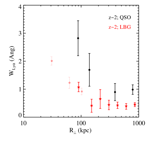
Figure 18.— Comparison of the excess equivalent width of H I Ly$\alpha$ absorption relative to the ambient IGM for the environments surrounding $z\sim 2$ quasars (black; $W_{\rm Ly\alpha}^{\rm stack}$ values from this paper) and the $z\sim 2$ Lyman break galaxies (red; Steidel et al., 2010; Rakic et al., 2012). At all proper impact parameters $R_{\perp}$, the H I absorption associated to the galaxies hosting quasars is stronger. This is consistent with the result that quasars reside in more massive halos than those hosting LBGs at $z\sim 2$.

These quasar host halo masses exceed the halo masses estimated for the $z\sim 2-3$ star-forming galaxy population termed Lyman break galaxies (LBGs; Steidel et al., 1996). Clustering analyses and halo occupation models for the LBGs yield mass estimates and limits ranging from $M_{\rm halo}^{\rm LBG}\approx 10^{11.4}-10^{12}{\rm\ M}_{\odot}$ (e.g. Adelberger et al., 2005b; Bielby et al., 2013). Within $\Lambda$CDM, therefore, one predicts that $z\sim 2-3$ quasars will exhibit greater H I Ly$\alpha$ absorption than LBGs at the same proper separation. Figure 18 compares the equivalent width of H I Ly$\alpha$ from our stacked spectra against comparable measurements derived from LBGs (Steidel et al., 2010; Rakic et al., 2012). At all proper impact parameters $R_{\perp}$, the environments surrounding $z\sim 2$ quasars show greater H I Ly$\alpha$ absorption than that of the LBGs (see also QPQ5). The immediate conclusion is that quasar environments have greater overdensities on these scales. As emphasized in QPQ5, this includes $R_{\perp}<100$ kpc where one likely intersects the virial radius and current numerical simulations tend to predict less cool gas in massive halos (e.g. Kereš et al., 2009; Stewart et al., 2011; van de Voort & Schaye, 2012; Fumagalli et al., 2013a).

To further explore these results in the context of $\Lambda$CDM, we have compared our observations against outputs from the cosmological simulation of a massive dark matter halo at $z>2$. Specifically, we have produced simulated mock spectra from a high-resolution simulation of the formation of a massive halo at $z\sim 2.4$ obtained with the RAMSES code (Teyssier, 2002) as described in detail in appendix B of Cantalupo et al. (2012). The simulation has a box size of 40 comoving Mpc (corresponding to about 2800  km s^-1 at at $z\sim 2.5$) and a maximum spatial (mass) resolution of about 180 proper pc ($1.8\times 10^{6}{\rm\ M}_{\odot}$) at $z\sim 2.4$ using adaptive mesh refinement. The box has been centered on the most massive halo at $z=2.4$, $M_{\mathrm{halo}}\sim 6\times 10^{12}{\rm\ M}_{\odot}$, as a representative host of a luminous quasar. We include in the hydro-simulation the photo-ionization from the cosmic UV background (Haardt & Madau 2012), star formation, metal enrichment, metal cooling and supernova feedback (Cantalupo et al., 2012).

The hydro-simulation has been post-processed with the radiative transfer code RADAMESH (Cantalupo & Porciani, 2011) to model the effect of the cosmic UV background. We do not discuss here models that include radiation from the f/g quasar. We have simulated 7500 mock spectra with randomly distributed orientations and impact parameters with respect to the quasar host. The simulated spectra include the effect of gas peculiar velocities and the errors on the quasar systemic redshifts (randomly generated from a Gaussian distribution with $\sigma_{z}=520{\rm km~{}s^{-1}}$, the typical value associated with our quasar sample). Note, however, that these effects are practically negligible given the large size of the velocity window used for the flux averaging (2000  km s^-1). The simulated absorption shows good agreement with the observations on large scales ($R_{\perp}\gtrsim 200$ kpc), as shown in Figure 19. In this respect the observations are consistent with quasars tracing massive halos at $z\sim 2.5$. On the other hand, it is apparent that our ‘standard’ simulation shows too little absorption on small scales, especially within 200 proper kpc from the quasar. Even without quasar radiation, the model does not show the observed steep increase in $\delta_{<F_{2000}>}$ on these scales.

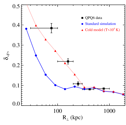
Figure 19.— Comparison of $\delta_{\langle F\rangle}$ values measured from the QPQ6 dataset (black points) with predictions from simulations of a massive halo at $z=2.4$ ($M_{\rm halo}\approx 10^{12.8}{\rm\ M}_{\odot}$; Cantalupo et al., 2012). The solid blue curve shows the standard output where we have neglected any radiation from a central quasar. This model matches the data well at large impact parameters $(R_{\perp}\gtrsim 200$ kpc) but under-predicts the absorption on scales comparable to the virial radius. We conclude that such simulations underpredict the amount of cool gas within the CGM of massive galaxies (see also Fumagalli et al., 2013a). As a simple attempt to reproduce the data, we generated a second, toy model where the gas within 200 kpc is restricted to $T\leq 10^{4}$ K (red, dotted curve). This provides a better match to the observations on small scales. Future work will explore the astrophysical processes within the CGM of massive galaxies that may reproduce the implied reservoir of cool gas.

We note that $R_{\perp}\sim 200$ kpc corresponds to about one virial radius for the selected, massive halo. Simulated gas within this radius is shock-heated to very high temperatures ($\sim 10^{7}$ K) and therefore highly ionized by collisional ionizations. The significant lack of absorption in the simulated spectra may be an indication that the simulations are missing a population of small, cold clumps within the hot gas, due to resolution or other effects possibly related to multi-phase gas physics or metal mixing. We have therefore considered a toy model in which, as an extreme case, we have forced all the gas within the halo to have an initial, maximum temperature of $10^{4}$ K (without changing its density), before applying the radiative transfer. In this case, the gas is photo-ionized and the contribution from collisional excitations is neglected. The resulting $\delta_{\langle F\rangle}$ values indicated by the red dotted line in Figure 19, are now in much better agreement with the QPQ6 data. Although this ‘cold’ model is clearly an oversimplification and it does not represent a univocal solution to the discrepancy with data, it suggests that the halo contains a sufficient reservoir of gas but that a non-negligible fraction should be much cooler than predicted by our standard model. This cold gas may be present in form of small, dense clumps that are not resolved by our simulation. Higher resolution and additional astrophysical processes, e.g. a proper treatment of metal mixing and cooling in a multi-phase halo gas, may be required to resolve the discrepancy with the data. We will explore these processes in future works.

6.4. Clustering of H I Absorbers with $z\sim 2$ Quasars in the Transverse Dimension

In this sub-section, we measure the cross-correlation signal of strong H I absorbers with quasars to explore the physical nature of these systems. The formalism was introduced and applied in QPQ2 to measure the quasar-absorber correlation function $\xi_{\rm QA}$ of H I absorbers transverse to quasar sightlines. In that paper, we measured a large correlation length $r_{0}=9.2^{+1.5}_{-1.7}h^{-1}{\rm\ Mpc}$ for systems with $N_{\rm HI}\geq 10^{19}\,{\rm cm^{-2}}$, assuming $\xi_{\rm QA}\propto(r/r_{0})^{\gamma}$ with $\gamma=1.6$. We compared this result with measurements along the line-of-sight and concluded that these absorption systems were anisotropically clustered around quasars. We further surmised that the gas detected in b/g sightlines is typically not illuminated by the quasar, either because of anisotropic emission or episodic variability (we currently favor the former). Using the QPQ6 dataset, we update this calculation with a much larger pair sample and also extend the analysis to absorbers with lower H I column densities. A description of the $N_{\rm HI}$ measurements was given in $\S$ 4.2 (see also the Appendix).

6.4.1 Clustering Analysis

Define $\xi_{\rm QA}(r)$ to be the cross-correlation function that describes clustering of absorbers to quasars. Given the small sample size in QPQ2, we parameterized the correlation function as a power-law $\xi_{\rm QA}=(r/r_{0})^{-\gamma}$ with a fixed exponent, $\gamma=1.6$, following standard results from galaxy-galaxy clustering (e.g. Adelberger et al., 2005b). With QPQ6, we have analyzed $N_{\rm pair}=393$ quasar pairs for strong H I absorbers at comoving impact parameters ranging from $R_{\perp}^{\rm com}\approx 0.1-3h^{-1}{\rm\ Mpc}$ and $z_{\rm fg}<3$. We begin by fixing $\gamma=1.6$, test whether this provides a good description of the observations, and then allow $\gamma$ to vary.

In practice, we have surveyed absorption systems in spectral windows $\pm 1500{\rm km~{}s^{-1}}$ around $z_{\rm fg}$ at a range of comoving impact parameters $R_{\perp}^{\rm com}$. Following the formalism in QPQ2, we evaluate $\xi_{\rm QA}(r)$, by maximizing the likelihood of the data for observing $N_{\rm sys}$ absorption systems amongst the $N_{\rm pair}$ pairs, where the probability of finding an absorber in the redshift interval $\Delta z=2(1+z)/(\Delta v/c)$ at separation $R_{\perp}^{\rm com}$ is $P(R_{\perp}^{\rm com},z)=\ell_{q}\,\Delta z$ with $\Delta v=1500{\rm km~{}s^{-1}}$ and $\ell_{q}$ evaluated along the sightline. Note that $P(R_{\perp}^{\rm com},z)=\ell_{q}\,\Delta z$ is equivalent to the covering fraction $f_{C}$ which we evaluated in $\S$ 4.2 for optically thick gas (and in proper units). Specifically, we have

$$\ell_{q}(z,R_{\perp}^{\rm com},\Delta v)=\ell_{\rm IGM}(z)\;[1+\chi_{\perp}(R_{\perp}^{\rm com},\Delta v)]$$ (5)

where $\ell_{\rm IGM}(z)$ is the incidence of absorbers in a random region of the universe,

$$\chi_{\perp}(R_{\perp},\Delta v)\approx\frac{aH(z)}{2\Delta v}\int\limits_{-\Delta v/[aH(z)]}^{\Delta v/[aH(z)]}\,dZ\,\xi_{\rm QA}(\sqrt{R_{\perp}^{2}+Z^{2}})\;\;\;,$$ (6)

$a\equiv 1/(1+z)$, and $Z$ is the comoving distance along the sightline relative to $z_{\rm fg}$.

To compute $\ell_{\rm IGM}(z)$, we adopt the $f(N_{\rm HI},X)$ distribution of O’Meara et al. (2013) at $z\approx 2.5$ assuming a redshift evolution $(1+z)^{3/2}$ and evaluate $\ell_{\rm IGM}(z)=\ell(X)_{\rm IGM}dX/dz$ with

$$\frac{dX}{dz}=\frac{H_{0}}{H(z)}(1+z)^{2}\;\;\;,$$ (7)

and

$$\ell_{\rm IGM}(X)=\int\limits_{N_{\rm HI}^{\rm min}}^{N_{\rm HI}^{\rm max}}f(N_{\rm HI},X)\,dN_{\rm HI}\;\;\;.$$ (8)

We perform this analysis for three absorption-line samples: (1) the damped Ly$\alpha$ systems (or DLAs) with $N_{\rm HI}\geq 10^{20.3}\,{\rm cm^{-2}}$. The QPQ6 dataset is complete for such systems. The O’Meara et al. (2013) results give $\ell^{\rm DLA}_{\rm IGM}(z)\approx 0.2[(1+z)/(1+2.5)]^{2.1}$, in good agreement with Prochaska et al. (2008); (2) super Lyman limit systems (or SLLS) with $10^{19}\,{\rm cm^{-2}}\leq N_{\rm HI}\leq 10^{20.3}\,{\rm cm^{-2}}$. An evaluation of equation 8 gives $\ell^{\rm SLLS}_{\rm IGM}(z)\approx 0.44[(1+z)/(1+2.5)]^{2.1}$. As discussed in $\S$ 4.2, we have taken a conservative approach towards identifying SLLS in these lower resolution data. Therefore, our estimate of the clustering signal may be an underestimate; (3) optically thick systems (or LLS) with $N_{\rm HI}\geq 10^{17.3}\,{\rm cm^{-2}}$, corresponding to $\tau\geq 2$ at the Lyman limit. As described in $\S$ 4.2, we do not observe directly the Lyman limit of the gas but infer that systems are optically thick based on several criteria. Evaluating the O’Meara et al. (2013) distribution function, we find $\ell^{\rm LLS}_{\rm IGM}(z)\approx 1.05[(1+z)/(1+2.5)]^{2.1}$, in good agreement with Ribaudo et al. (2011).

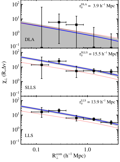
Figure 20.— The black data points show binned evaluations of the transverse cross-correlation function $\chi_{\perp}$ as a function of comoving impact parameter for DLA, SLLS, and LLS absorption systems with quasars. The solid blue curves show the best-fit model for $\xi_{\rm QA}=(r/r_{0})^{-\gamma}$ with $\gamma=1.6$, evaluated along the sightline at that impact parameter (Equation 6). These models, derived from a maximum likelihood analysis, offer an excellent description of the observations. The gray shaded region indicates uncertainty in the models (we have adopted a 25% systematic error). The clustering amplitude for DLAs matches previous estimates and is consistent with gas tracing the ISM of individual galaxies. The very large amplitudes for the LLS/SLLS imply a bias in the environments of massive galaxies that enhances the formation of optically thick gas. We propose that this gas arises in the overdense but uncollapsed large-scale structures (e.g. filaments) of the cosmic web around massive galaxies. For comparison, we show the galaxy-quasar cross-correlation function from Trainor & Steidel (2012) as a dotted red line.

The results from these analyses are presented in Figure 20 which shows binned evaluations of the transverse correlation function $\chi_{\perp}$ evaluated in logarithmic bins of separation by comparing the observed incidence of systems relative to random expectation (see QPQ2). We overplot on these evaluations the best-fit models for $\xi_{\rm QA}$, converted into $\chi_{\perp}$ (Equation 6). These models were derived using our maximum likelihood estimator and the uncertainties were determined using a Monte Carlo method (see QPQ2 for details). For $\gamma=1.6$, we recover clustering amplitudes $r^{\rm DLA}_{0}=3.9\pm 2.3h^{-1}{\rm\ Mpc}$, $r^{\rm SLLS}_{0}=15.3\pm 1.5h^{-1}{\rm\ Mpc}$, and $r^{\rm LLS}_{0}=14.6\pm 0.8h^{-1}{\rm\ Mpc}$. All of the observations are well described by these models; a Kolmogorov-Smirnov (KS) test comparing the observed $R_{\perp}^{\rm com}$ distribution of the H I systems with the distribution predicted from the best-fit models (adopting the QPQ6 distributions of $R_{\perp}^{\rm com}$ and $z_{\rm fg}$) gives $P_{\rm KS}\approx 0.25$ for the DLAs and $P_{\rm KS}>0.9$ for the SLLS and LLS.

Our results confirm the primary conclusion of QPQ2, that strong H I absorbers are highly correlated with quasars in the transverse dimension. In fact, for the LLS and SLLS populations (which overlap significantly) we derive clustering amplitudes higher than those reported in QPQ2, even exceeding quasar-quasar and quasar-galaxy clustering at $z\sim 2.5$ (Shen et al., 2007; Trainor & Steidel, 2012). To emphasize the difference, we overplot the projected cross-correlation function of quasar-galaxy clustering in Figure 20 using the results of Trainor & Steidel (2012).

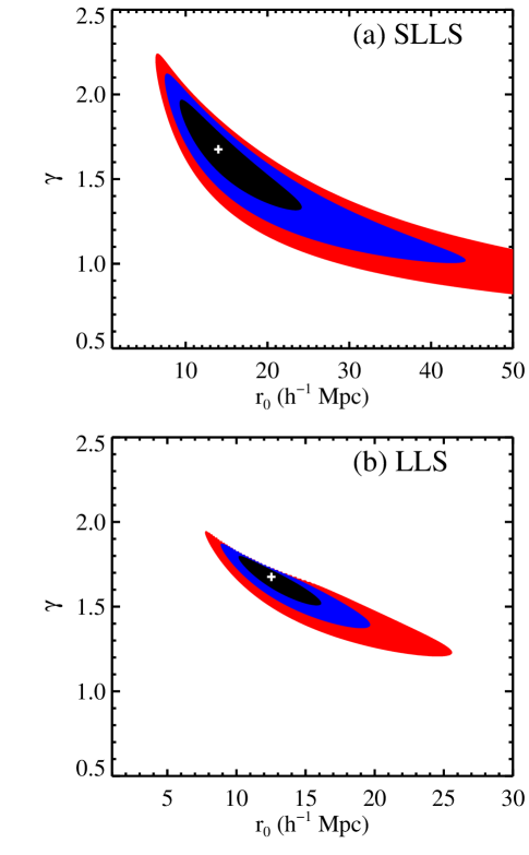
Figure 21.— Confidence contours (black, blue, red for 68.3%, 95.4%, and 99.7% respectively) for clustering fits $\xi_{\rm QA}=(r/r_{0})^{-\gamma}$ to the (a) SLLS and (b) LLS around quasars. There is an obvious degeneracy between the $r_{0}$ and $\gamma$, although the results are reasonably well constrained. Integrating over each parameter we recover $r_{0}^{\rm SLLS}=14.0^{+7.6}_{-2.7}h^{-1}{\rm\ Mpc}$ with $\gamma^{\rm SLLS}=1.68^{+0.06}_{-0.13}$ for the SLLS and $r_{0}^{\rm LLS}=12.5^{+2.7}_{-1.4}h^{-1}{\rm\ Mpc}$ with $\gamma^{\rm LLS}=1.68^{+0.14}_{-0.30}$ for the LLS.

The formal error bars for the SLLS/LLS are very small, owing to the large clustering signal (see QPQ2) and our having fixed $\gamma=1.6$. Indeed $\gamma$ and $r_{0}$ are highly correlated. In Figure 21, we present the confidence contours for $\gamma$ and $r_{0}$ for the LLS and SLLS having allowed each parameter to vary freely. For the SLLS, the results give $r_{0}^{\rm SLLS}=14.0^{+7.6}_{-2.7}h^{-1}{\rm\ Mpc}$ with $\gamma^{\rm SLLS}=1.68^{+0.06}_{-0.13}$ at 68% c.l. Similarly, the analysis gives $r_{0}^{\rm LLS}=12.5^{+2.7}_{-1.4}h^{-1}{\rm\ Mpc}$ with $\gamma^{\rm LLS}=1.68^{+0.14}_{-0.30}$ for the LLS. These results are more reflective of the uncertainty in the clustering amplitude. Furthermore, the Monte Carlo error estimate does not reflect uncertainty in the $N_{\rm HI}$ measurements, neither statistical nor systematic (see $\S$ 4.2). We also estimate an uncertainty of $\approx 20\%$ in the background incidence which affects the clustering measurements. Considering these effects together, we recommend adopting an $\approx 25\%$ uncertainty for our best-fit $r_{0}$ values.

Of greatest importance to the discussion that follows is the enhancement in SLLS (and LLS) at large separations. As such, we have carefully scrutinized this result (QPQ5 focused on small scales). For the SLLS, we discovered 14 systems in the QPQ6 dataset at $R_{\perp}^{\rm com}>1h^{-1}{\rm\ Mpc}$ where only 2.2 were predicted. Of these 14, at least 10 show strong low-ion absorption indicative of SLLS and we consider them secure. Restricting to the 10 systems, we recover $r_{0}^{\rm SLLS}=14.7h^{-1}{\rm\ Mpc}$ for $\gamma=1.6$. Similar conclusions are drawn for the LLS. We conclude that $r_{0}>10h^{-1}{\rm\ Mpc}$ is a robust result for the clustering of SLLS and LLS for $\gamma<1.8$.

6.4.2 Implications for H I Absorbers and the CGM

The previous sub-section presented new measurements on the clustering of strong H I systems to quasars, as measured from the QPQ6 survey, corresponding to comoving separations of $R_{\perp}^{\rm com}<2.5h^{-1}{\rm\ Mpc}$. We remind the reader that quasars inhabit massive halos inferred (in part) from the large quasar-quasar auto-correlation length ($r_{0}=8.4h^{-1}{\rm\ Mpc}$ for $\gamma=2$; White et al., 2012). This sets a reference for which to consider our results. In principle, one may combine the quasar-absorber cross-correlation with the auto-correlation function to estimate the mass of the dark matter halos hosting the absorbers. This requires, however, that the absorbers trace the dark matter density field deterministically and that the analysis be performed on the same scales. In general, absorbers are believed to be hosted by dark matter halos that are less biased than quasars, such that the quasar-absorber cross-correlation length is expected to be smaller than the quasar auto-correlation.

Previous studies on absorber clustering have focused on galaxies, in part because the latter have a much higher comoving number density than quasars. At low redshift, such measurements have been used to examine the origin of strong Mg II absorption (e.g. Bouché et al., 2004; Tinker & Chen, 2008; Padilla et al., 2009) and the nature of the Ly$\alpha$ forest (Chen et al., 2005; Tejos et al., 2012). At $z\sim 2$, studies have examined the link between C IV gas and LBGs (Adelberger et al., 2005a; Martin et al., 2010) and have placed constrains on the halo masses for DLAs (Bouché & Lowenthal, 2004; Cooke et al., 2006a). Regarding quasar-absorber clustering, in addition to QPQ2, Wild et al. (2008) measured the Mg II and C IV clustering with quasars at $z\sim 1$ and 2 respectively on large, transverse scales ($R_{\perp}^{\rm com}\gg 1h^{-1}{\rm\ Mpc}$). The clustering lengths ($r_{0}\approx 5h^{-1}{\rm\ Mpc}$) were used to infer that quasars are hosted by halos with masses $M>10^{12.5}{\rm\ M}_{\odot}$ at $z\sim 2$ and over $10^{13}{\rm\ M}_{\odot}$ at $z\sim 1$. The quasar-absorber cross-correlation amplitude also offers insight into the physical nature and origin of strong H I absorbers and on astrophysical processes for cool gas in massive halos.

Consider first our results for the DLAs. The estimated clustering length is consistent with previous estimates from LBG-DLA cross-correlation analyses performed on similar scales (Cooke et al., 2006a). Formally, $r_{0}^{\rm DLA}=3.8h^{-1}{\rm\ Mpc}$ is preferred and the correlation length is restricted to $r_{0}^{\rm DLA}<9h^{-1}{\rm\ Mpc}$ (95% c.l.) for $\gamma=1.6$. Our results are consistent with models where DLAs trace dark matter halos (i.e. galaxies; Pontzen et al., 2008) and the clustering amplitude implies characteristic masses of $M_{\rm halo}^{\rm DLA}\sim 10^{11}-10^{12}{\rm\ M}_{\odot}$ (Lee et al., 2011; Font-Ribera et al., 2012). There is no signature of the so-called one-halo term where $\xi_{\rm QA}(r)$ shows excess small-scale clustering due to satellites of the central halo, but we caution that this conclusion is tempered by the small sample size. In summary, the results for DLAs follow one’s expectation for gas tracing galaxies within common dark matter halos, i.e. the ISM of star-forming galaxies.

In contrast to the DLAs, the LLS and SLLS exhibit very large clustering lengths, e.g. $r_{0}^{\rm SLLS}>10h^{-1}{\rm\ Mpc}$, which even exceeds the correlation lengths for quasar-quasar and quasar-galaxy clustering at $z\sim 2$. Naively, following the discussion above, one might infer that these optically thick absorbers would need to trace amongst the most massive dark matter halos in the Universe ($M>10^{13}{\rm\ M}_{\odot}$). This assertion is easily dismissed, however, because such halos are so exceedingly rare at $z\sim 2$ that they could not possibly account for the observed incidence of optically thick gas. For example, given the low number density of halos with $M>10^{13}{\rm\ M}_{\odot}$, these would need to have an effective area $A_{\rm eff}>2{\;\times\;10^{6}}\,{\rm kpc^{2}}$ corresponding to a typical radius of 800 kpc to match the LLS incidence (see $\S$ 6.5 for further details). This would require a 100% covering factor of SLLS to well beyond the virial radius in these massive halos. We conclude that at the small scales probed here ($R_{\perp}<2.5h^{-1}{\rm\ Mpc}$) from luminous QSOs, LLSs are no longer simple biased tracers of the underlying dark matter.

Instead, we infer that the large $r_{0}$ values are driven by astrophysical processes which bias the $\approx 1$ Mpc environments surrounding quasars to preferentially exhibit optically thick gas. On small scales, i.e. within the virial radius, the clustering signal could be driven by gas within the CGM of the host halo. The clustering observed on larger scales, however, implies the presence of a dense, self-shielding medium giving rise to LLS/SLLS which lies between dark matter halos. We hypothesize that this gas is located within the large-scale structures (e.g. filaments) that connect the massive halo to its neighbors. Because we do not observe such clustering in the DLAs, the structures must have surface densities preferentially below the $N_{\rm HI}=10^{20.3}\,{\rm cm^{-2}}$ threshold.

We now discuss several such scenarios that may explain the large clustering amplitude, focusing first on the inner regions $r\lesssim r_{\rm vir}$ ($\approx 160$ kpc for a halo with $M\approx 10^{12.5}{\rm\ M}_{\odot}$ at $z=2.5$). Might the large clustering length (and correspondingly high covering fraction) of optically thick gas result from satellite galaxies in the central halo? Indeed, quasars reside in massive halos and $\Lambda$CDM clustering predicts an abundance of such satellite galaxies (e.g. Maller et al., 2001). If we confine the gas from such satellites to lie within their halos, however, one finds a small covering fraction and a correspondingly small clustering amplitude (e.g. QPQ3; Tumlinson et al., 2013). For example, one predicts an average of 5 satellites with $M>10^{10}{\rm\ M}_{\odot}$ within the virial radius of halos with $M_{\rm halo}=10^{12}-10^{13}{\rm\ M}_{\odot}$ at $z=2.5$ (Behroozi et al., 2013). Even if we assumed that optically thick gas extended uniformly to a radius of 20 kpc within each satellite, these would cover $\lesssim 10\%$ of the projected area of the central halo. We reached the same conclusion in QPQ3 based on analysis of the observed quasar-galaxy cross-correlation function. In addition, satellite galaxies should also contribute to DLA absorption and significant quasar-DLA clustering which is not observed.

If gas within satellite galaxies is insufficient, one must conclude that this optically thick gas comprises the ambient circumgalactic medium (CGM) of the central halo. But from where did this material originate? As discussed in QPQ5, the high incidence of strong metal-line absorption indicates the gas is chemically enriched. This requires that a non-negligible fraction of the material has previously cycled through a galaxy. The total gas mass implied is large ($M>10^{10}{\rm\ M}_{\odot}$), and it may thus be unlikely that the majority of this CGM was stripped/expelled from the halo’s satellite galaxies. Indeed, numerical simulations of galaxy formation currently predict that the majority of dark matter and baryons accrete onto halos in diffuse streams (Kereš et al., 2005; Dekel et al., 2009; Brooks et al., 2009). On the other hand, such streams alone are unlikely to reproduce the clustering signal ($\S$ 6.3, Fumagalli et al., 2013a). Material driven from the galaxy hosting the f/g quasar, e.g. via supernovae or AGN feedback, may also inject gas and metals into the surrounding halo. A fraction of this material may be cool and could be optically thick, but we question whether it can travel to large radii given the implied energetics (QPQ3). We suspect that none of these effects (streams, satellites, expelled gas) alone can reproduce the observations. Absent any other obvious effects (e.g. the condensation of cool gas out of a hot halo), we contend that they all must contribute to match the observations. We await the output of new ‘zoom-in’ simulations of massive halos at $z\sim 2$ to further explore these issues (e.g. Cantalupo et al., 2012; Fumagalli et al., 2013a).

Another question that follows relates to the survival of this CGM gas: Is it ephemeral, i.e. does it require constant replenishment? If the gas exists outside satellites and their dark matter halos, we may assume it is not self-gravitating. For these ‘clouds’ to avoid rapid dissipation through adiabatic expansion, we propose that it be embedded within a warm/hot medium that offers pressure confinement (e.g. QPQ3). Previous work has described a range of physical processes that can and should destroy cool gas clouds within a hot halo (e.g. Mo & Miralda-Escude, 1996; McDonald & Miralda-Escudé, 1999; Maller & Bullock, 2004; Schaye et al., 2007). These would apply to the CGM of our massive halos, albeit with a presumably hotter halo (previous work considered lower mas halos with virial temperatures $\sim 10^{6}$ K) and higher mean density than average. In QPQ3, we demonstrated that such clouds could exist in pressure equilibrium with the hot virialized tenuous plasma predicted to be present in the massive dark matter halos hosting quasars. Evaluating the survival time of such clouds and the processes that may generate a new population deserves focused, numerical studies that include radiative-transfer coupled to the hydrodynamics.

While one may evoke various astrophysical mechanisms within the CGM of the central halo to explain the high clustering signal on small scales ($r<r_{\rm vir}$), we reemphasize that the observations show substantial clustering even at $R_{\perp}^{\rm com}\approx 3h^{-1}{\rm\ Mpc}$. And again, the measured amplitude likely exceeds anything that could be produced by the LLSs tracing the underlying dark matter, because in order to reproduce this amplitude the LLSs would have to exist in extremely massive halos implying unphysically large cross-sections. Instead, we hypothesize that a baryonic bias exists for optically thick gas on proper scales of $\sim 1$ Mpc. We further speculate that this gas arises in the large-scale structures (e.g. filaments) surrounding massive halos. The gas within these overdense regions self-shields and gives rise to SLLS and LLS (e.g. McQuinn et al., 2011; Altay et al., 2011). While lower mass halos should also exhibit extended structures (albeit on smaller scales), the amplitude of their overdensities are lower and may be insufficient to produce optically thick gas. We encourage future observational and theoretical work to (a) confirm the clustering signal at $R_{\perp}^{\rm com}\approx 3h^{-1}{\rm\ Mpc}$ and extend it to larger impact parameters; and (b) explore the likelihood that SLLS/LLS preferentially arise in the large-scale structures surrounding massive halos at $z\sim 2$.

There are a few additional points to emphasize. First, the strong clustering signal implies a bias of SLLS/LLS to massive halos. Under the expectation that such environments exhibit preferentially higher metallicity, this may bias the absorbers to have higher enrichment. Indeed, one observes a remarkable number of SLLS with solar or super-solar abundances (e.g. Péroux et al., 2006; Prochaska et al., 2006), perhaps exceeding the incidence of high-metallicity DLAs (Péroux et al., 2007; Dessauges-Zavadsky et al., 2009; Kaplan et al., 2010). Indeed, this has led to speculations that SLLS trace more massive galaxies (Kulkarni et al., 2010). Second, there is an apparent mass dependence to the presence of optically thick gas. Although the LLS cross-correlation with LBGs has not yet been measured, the observed covering factor of LLS is considerably lower for LBGs at the same proper scales than for quasars (QPQ5). Similarly, Adelberger et al. (2005a) measured the cross-correlation of strong C IV systems (which may preferentially trace strong H I absorbers) and measured $r_{0}\sim 4h^{-1}{\rm\ Mpc}$ on scales of a few $h^{-1}{\rm\ Mpc}$. This is much smaller than what we record for optically thick gas and quasars, although we do caution that our SLLS show relatively modest C IV equivalent widths (QPQ5).

Third, the significant clustering of optically thick gas has implications for the attenuation of quasar ionizing radiation and the resultant intensity of the UV background. The most important effect of LLS clustering would be to underestimate the mean free path of photons (if one were to neglect it). Lastly, it is worth considering whether any of these results are biased by the presence of a luminous quasar. For example, if the quasar’s radiation field illuminates gas throughout the environment, it should suppress optically thick gas and thereby reduce the clustering amplitude (and covering fraction). Such a bias would only accentuate the conclusions drawn above. On the other hand, one could speculate that quasars shine only during episodes of intense galaxy formation, e.g. during galaxy-galaxy mergers, which could enhance the presence of cool gas in the environment. We consider this unlikely because the signal we observe extends to Mpc whereas the fueling of AGN occurs on pc scales. It would be remarkable for such processes to be so tightly coupled. Furthermore, estimates of the star-formation rates of galaxies hosting luminous quasars do not indicate extreme activity (Santini et al., 2012; Rosario et al., 2013).

6.5. The Contribution of Massive Halos to QAL Systems

Quasar absorption line (QAL) systems with the largest H I column densities have been associated with galaxies and the dark matter halos within which they reside. This includes the damped Ly$\alpha$ systems (DLAs, $N_{\rm HI}\geq 10^{20.3}\,{\rm cm^{-2}}$; Wolfe et al., 2005), the super Lyman limit systems (SLLS, $N_{\rm HI}\geq 10^{19}\,{\rm cm^{-2}}$; Péroux et al., 2005; O’Meara et al., 2007), and the optically thick Lyman limit systems (LLS, $N_{\rm HI}\gtrsim 10^{17}\,{\rm cm^{-2}}$; Prochaska et al., 2010; Fumagalli et al., 2013b). Their association to galaxies is motivated by the nearly ubiquitous detection of heavy elements (Rafelski et al., 2012; Prochaska et al., 2010; Péroux et al., 2005; Fumagalli et al., 2011a) and the expectation that such high $N_{\rm HI}$ values may only be achieved within collapsed structures. Such inferences are supported by analysis of cosmological simulations (e.g. Pontzen et al., 2008; Faucher-Giguère & Kereš, 2011; Fumagalli et al., 2011b; Erkal et al., 2012; Rahmati et al., 2013).

It is of great interest is to establish the masses of the halos hosting these absorption systems. In $\S$ 6.4, we measured the clustering of these absorbers with quasars in the transverse dimension. Our results require that these massive halos contribute a non-zero fraction of strong H I absorption systems. On the other hand, massive halos are sufficiently rare that their integrated contribution to the incidence of these absorbers may be small. By comparing the contribution of massive halos to the cosmological incidence of these QAL systems, one may in turn constrain their host halo masses. For example, if massive halos have insufficient cross-section to LLS absorption, then this gas must manifest in alternate regions of the universe.

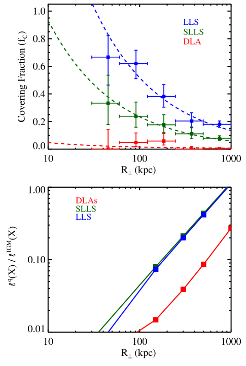
Figure 22.— (top): Binned evaluations of the covering fraction $f_{C}$ for strong H I absorption systems (LLS, SLLS, DLAs) as a function of proper impact parameter $R_{\perp}$ from a luminous $z\sim 2$ quasar. Specifically, $f_{C}$ is defined as the fraction of sightlines at $R_{\perp}$ that show at least one such absorber in a velocity window $\Delta v=\pm 1500{\rm km~{}s^{-1}}$ around the f/g quasar redshift. The dashed curves show estimations of $f_{C}$ from the evaluation of the cross-correlation functions derived in $\S$ 6.4 and shown in Figure 20. (bottom): The solid curves show the fractional contribution of gas in the environments of $z\sim 2$ luminous quasars to the total incidence of strong H I absorbers (LLS, SLLS, DLAs). These assume the $f_{C}$ evaluations shown above and that quasars trace dark matter halos with $M_{\rm halo}^{\rm min}\geq 10^{12}{\rm\ M}_{\odot}$. The curves also assume that $f_{C}=1$ for $R_{\perp}^{\rm min}\leq 10$ kpc. DLAs rarely occur within a few hundred kpc of massive halos. In contrast, quasar environments contribute significantly to optically thick gas (LLS, and especially the SLLS). For an assumed virial radius $r_{\rm vir}=150$ kpc, massive halos contribute approximately 10% of the incidence of these optically thick absorbers. The contribution of the extended environment ($\sim 1$ Mpc) approaches 100%. This suggests that all such gas lies within $\approx 1$ Mpc of a massive halo, e.g. neighboring and lower mass dark matter halos and/or the large-scale structures that connect these halos.

For a population of halos with a comoving number density $n^{\rm com}$ and an effective, physical cross-sectional area $A^{\rm eff}$ to a given H I column density, the incidence per unit absorption length $dX$ (Equation 7) is given by

$$\ell(X)=\frac{c}{H_{0}}\,n^{\rm com}\,A^{\rm eff}\;\;\;.$$ (9)

We will assume that quasars occupy all halos with masses greater than a minimum value $M_{\rm halo}^{\rm min}$. Assuming a $\Lambda$CDM cosmology and standard Press-Schecter analysis (e.g. Bardeen et al., 1986; Dekel & Birnboim, 2006), this sets $n^{\rm com}$ at a given redshift. For the effective area, we adopt $A^{\rm eff}=f_{C}\,\pi R_{\perp}^{2}$ with $f_{C}$ the measured covering factor within $R_{\perp}$.

Figure 22a presents the evaluation of $f_{C}$ for LLS, SLLS, and DLAs from our QPQ6 dataset (see also Figure 10). For an evaluation of $f_{C}$ at any impact parameter, we may recast the cross-correlation functions measured in the previous sub-section in terms of a covering fraction. In comoving coordinates, $f_{C}$ at comoving impact parameter $R_{\perp}^{\rm com}$ is given by $f_{C}(R_{\perp}^{\rm com})=\ell_{q}(R_{\perp}^{\rm com},\Delta v)\Delta z$ with $\ell_{q}$ given by Equation 5 and we take $\Delta v=\pm 1500{\rm km~{}s^{-1}}$ to match our approach to assessing strong H I systems ($\S$ 4). The resultant $f_{C}$ curves assuming $\gamma=1.6$ are overplotted on Figure 22a, assuming $z=2.4$ to convert $R_{\perp}^{\rm com}$ to $R_{\perp}$ only to match the x-axis. These provide a good description of the observations (as expected).

We then calculate

$$A^{\rm eff}(R_{\perp})=\int\limits_{0}^{R_{\perp}}\,f_{C}(R_{\perp}^{\prime})\,2\pi R_{\perp}^{\prime}\,dR_{\perp}^{\prime}\;\;.$$ (10)

Note that we restrict $f_{C}\leq 1$ and we have set $f_{C}=1$ at impact parameters $R_{\perp}^{\rm min}\leq 10$ kpc for all absorbers to account for the ISM of a presumed host galaxy. This primarily impacts the results for the DLAs.

Figure 22b illustrates the fractional contribution of massive halos to the observed incidence of strong H I absorbers evaluated at several characteristic impact parameters: 30 kpc, 150 kpc (corresponding to approximately one virial radius $r_{\rm vir}$), 300 kpc ($\approx 2r_{\rm vir}$), 500 kpc, and 1 Mpc. All of the curves assume $M_{\rm halo}^{\rm min}=10^{12.5}{\rm\ M}_{\odot}$, giving $n=1.2{\;\times\;10^{-4}}$ halos Mpc^-3 (comoving) at $z=2.4$. For the incidence of LLS, SLLS, and DLAs in the ambient IGM, we have adopted $\ell^{\rm LLS}_{\rm IGM}(X)=0.3$, $\ell^{\rm SLLS}_{\rm IGM}(X)=0.13$, and $\ell^{\rm DLA}_{\rm IGM}(X)=0.055$ respectively. These values are drawn from traditional surveys of quasar absorption systems at $z\approx 2.4$ (Prochaska & Wolfe, 2009; O’Meara et al., 2007, 2013), increase by $\approx 50\%$ from $z=2$ to 3, and have approximately 20% uncertainty.

Consider first the DLAs. Figure 22b reveals that gas within the virial radius of massive halos ($M_{\rm halo}\geq 10^{12.5}{\rm\ M}_{\odot}$) does not contribute significantly to the total incidence of these strongest H I absorption systems. Even if we set $f_{C}=1$ for $R_{\perp}^{\rm min}\leq 20$ kpc, we find that $\ell^{\rm DLA}_{q}(X)$ is less than 5% of the total incidence at $R_{\perp}=150$ kpc, which matches or exceeds $r_{\rm vir}$ for the central halo. Unless the halos of quasars have suppressed DLA gas (contrary to all other inferences we have drawn), we conclude that the majority of DLAs must arise in halos with masses $M_{\rm halo}^{\rm DLA}\leq 10^{12.5}{\rm\ M}_{\odot}$. Font-Ribera et al. (2012) have measured the cross-correlation between the Ly$\alpha$ forest and DLAs and concluded that the latter may be hosted by more massive halos than previously derived from numerical simulations. In their fiducial model, which matches the clustering and incidence of DLAs (we caution this model is not unique), they assert that $10^{12}{\rm\ M}_{\odot}$ halos must have an effective area for DLAs of $A_{\rm eff}^{\rm DLA}=1400\,{\rm kpc^{2}}$. For the massive halos traced by quasars, we have identified 2 DLAs from the 38 pairs with $R_{\perp}<150$ kpc. This incidence is consistent with gas in the outer halo contributing a significant fraction of the $A_{\rm eff}$ value suggested by Font-Ribera et al. (2012), but clearly a much larger sample is required to offer a robust measurement.

In contrast to the DLAs, gas associated to massive galaxies contributes significantly to the SLLS and LLS populations. For $M_{\rm halo}^{\rm min}=10^{12.5}{\rm\ M}_{\odot}$, gas within $r\approx r_{\rm vir}$ of such massive halos yields $\approx 10\%$ of the SLLS in the Universe (Figure 22b). This is a remarkable result given that $M_{\rm halo}>10^{12.5}{\rm\ M}_{\odot}$ halos represent a small fraction of all dark matter halos at $z=2.4$, e.g. only $\sim{\;\times\;10^{-3}}$ of all halos with $M_{\rm halo}>10^{10}{\rm\ M}_{\odot}$. Despite being rare, their large physical size and covering fractions imply a substantial contribution to LLS. Even more remarkable, the results in Figure 22b indicate that the extended environment of massive halos (gas to $R_{\perp}\sim 1$ Mpc) yields an incidence of optically thick gas that roughly matches the IGM average. While there are substantial uncertainties in this estimate (e.g. $\ell_{q}(X)$ is sensitive to $M_{\rm halo}^{\rm min}$, $f_{C}$ has associated uncertainty), our quasar pair analysis implies that a substantial fraction of all optically thick gas occurs within the structures extended around massive galaxies at $z\sim 2$. This assumes, of course, that the condition of having a luminous quasar within these massive galaxies does not imply special characteristics for the gas on scales of 1 Mpc. If confirmed by future work, this result has significant consequences for our understanding of the LLS population, their contributed opacity of the IGM, and the attenuation of ionizing sources that generate the EUVB.

7. Summary

We have constructed a sample of 650 projected quasar pairs where spectra of the b/g quasar covers the H I Ly$\alpha$ line at the redshift of the f/g quasar. We have restricted the sample to data with ${\rm S/N}_{\rm Ly\alpha}>5.5$, proper separations at $z_{\rm fg}$ of $R_{\perp}\leq 1$ Mpc, and redshift separation such that H I Ly$\alpha$ of the f/g quasar lies in the rest wavelength interval $1030\,{\rm\AA}<\lambda_{r}<1200\,\rm\AA$ of the b/g quasar. The f/g quasars have redshifts $z_{\rm fg}=1.6-4.5$ with a median value of 2.34 and Bolometric luminosities ranging from $\approx 10^{45}-10^{47}\,{\rm erg\,s^{-1}}$. If these sources emit isotropically, their UV fluxes exceed the UV background by factors of 10 to 10,000. The quasar spectroscopy comprises a heterogeneous dataset drawn from SDSS, BOSS/DR9, and a diverse set of instruments on large-aperture telescopes. We have used these data to re-measure the f/g quasar redshifts and we have continuum normalized the b/g quasar spectra with an automated routine that mean flux regulates the data to the average H I Ly$\alpha$ opacity of the IGM (Lee et al., 2012).

We then proceeded to analyze these spectra to study the H I Ly$\alpha$ absorption in the $R_{\perp}\leq 1$ Mpc environment of $z\sim 2$ luminous quasars. The primary findings are:

• The 1 Mpc environments surrounding the massive galaxies which host luminous $z\sim 2$ quasars have enhanced H I Ly$\alpha$ opacity. For the complete sample, which has a median impact parameter of 725 Mpc, we find that $\delta_{\langle F\rangle}\equiv(\langle F\rangle_{\rm IGM}-\langle F\rangle^{2000})/\langle F\rangle_{\rm IGM}=0.09$.

• The excess H I absorption increases with decreasing $R_{\perp}$ consistent with the gas tracing a massive overdensity and not being illuminated by the f/g quasar. Analysis of composite spectra binned in intervals of $R_{\perp}$ yields an excess H I Ly$\alpha$ equivalent width: $W_{\rm Ly\alpha}^{\rm stack}=2.3\,{\rm\AA}(R_{\perp}/{\rm 100\,kpc})^{-0.46}$.

• Comparing the data against a numerical simulation of a massive halo (Cantalupo et al., 2012), we find good agreement on scales $R_{\perp}\gtrsim 200$ kpc but that the model shows much less absorption than observed on smaller scales. Current models of structure formation appear to underpredict the distribution of cool gas in the CGM of massive galaxies.

• The H I Ly$\alpha$ opacity around quasars exceeds that observed for LBGs (Rakic et al., 2012), consistent with the latter galaxies occupying systematically lower mass halos at $z\sim 2-3$.

• We analyzed the quasar-absorber cross-correlation function $\xi_{\rm QA}(r)$ to comoving impact parameter $R_{\perp}^{\rm com}\approx 2.5h^{-1}{\rm\ Mpc}$. Parameterizing $\xi_{\rm QA}(r)$ as a power-law $(r/r_{0})^{\gamma}$, we find $r^{\rm DLA}_{0}=3.9\pm 2.3h^{-1}{\rm\ Mpc}$ for a fixed $\gamma=1.6$ for DLAs, $r_{0}^{\rm SLLS}=14.0^{+7.6}_{-2.7}h^{-1}{\rm\ Mpc}$ with $\gamma^{\rm SLLS}=1.68^{+0.06}_{-0.13}$ for the SLLS, and $r_{0}^{\rm LLS}=12.5^{+2.7}_{-1.4}h^{-1}{\rm\ Mpc}$ with $\gamma^{\rm LLS}=1.68^{+0.14}_{-0.30}$ for the LLS. We estimate a systematic uncertainty of $\approx 20\%$ in these values.

• The amplitude for DLAs is consistent with previous galaxy-DLA cross-correlation measurements and follows expectation for gas tracing the ISM of galaxies. The very large clustering amplitude for optically thick gas (LLS, SLLS) indicates a strong bias toward such material in the environments of massive halos. We speculate that this gas arises predominantly in large-scale structures (e.g. filaments) that connect the central halo to neighboring dark matter halos on $\sim 1$ Mpc scales.

• We estimate that gas within the virial radius of massive halos $(M_{\rm halo}>10^{12.5}{\rm\ M}_{\odot}$) contribute $\sim 10\%$ of the observed optically thick gas at $z\sim 2.5$. In contrast, these halos yield less than 5% of DLAs. Extending to 1 Mpc, the environments of these massive halos may dominate the Universe’s Lyman limit opacity.

• Our observations of large enhancements in absorption in b/g sightlines provide compelling evidence for a large overdensity around the f/g quasar. Previous analyses of the line-of-sight proximity effect that have neglected this density enhancement will have systematically overestimated the EUVB intensity.

Future work will focus on (1) the metal-line absorption of gas in the quasar environment on both small ($R_{\perp}<r_{\rm vir}$) and large scales; (2) kinematics of the gas using a subset of the sample with precisely measured $z_{\rm fg}$ values from near-IR spectra; (3) an assessment of the transverse proximity effect; and (4) detailed analysis of echelle and echellette spectra of b/g spectra to study and analyze the CGM of quasar hosts. In parallel, we are pursuing and encouraging numerical simulations of massive galaxies at $z\sim 2$ to further explore the assembly of the most massive structures at early times.

APPENDIX: System Analysis

Figure 23 presents spectral regions centered on $\lambda_{\rm Ly\alpha}^{\rm fg}$ for a representative set of the sample, with the shaded region indicating the $1\sigma$ uncertainty in $z_{\rm fg}$. The figure describes the diversity of absorption apparent in the sample, both in terms of equivalent widths and velocity offsets of the absorbers from $z_{\rm fg}$. It also illustrates some of the subjectivity involved in defining systems. One occasionally has multiple absorption lines within the $\pm 1500{\rm km~{}s^{-1}}$ interval and the system nearest $z_{\rm fg}$ need not be the strongest. Nevertheless, the assignment of the ‘strongest line’ was generally unambiguous and we were relatively confident in defining the integration windows for the $W_{\rm Ly\alpha}$ measurements. All of the velocity regions and rest-frame Ly$\alpha$ equivalent widths $W_{\rm Ly\alpha}^{\rm line}$ for the H I systems are provided in Table 4.

The data at $\lambda_{\rm Ly\alpha}^{\rm fg}$ for those f/g quasars where we have measured an associated absorption system with $N_{\rm HI}\geq 10^{19}\,{\rm cm^{-2}}$ are presented in Figure 24 (see also $\S$ 4.2). Overplotted on these data are the Voigt profile fits and the shaded regions show our estimate of the $1\sigma$ uncertainty. Most of the systems with $N_{\rm HI}\approx 10^{19}\,{\rm cm^{-2}}$ exhibit low-ion absorption (e.g. QPQ5). All of the measurements are given in Table 4. Figure 25 presents a histogram of the measured $N_{\rm HI}$ values for the quasar pairs and compares them to the $N_{\rm HI}$ measurements for systems identified in the control sample. The distributions are similar but the control sample is much smaller owing to the large clustering signal of SLLS around quasars.

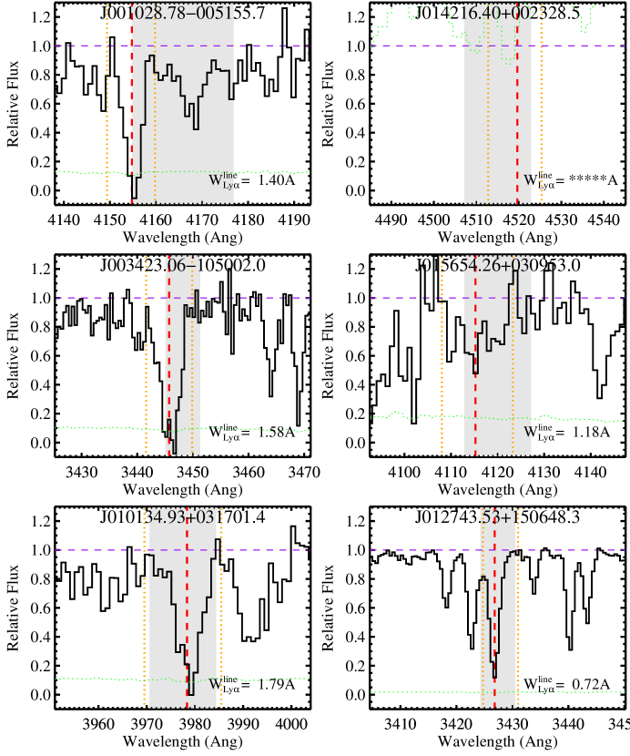
Figure 23.— The panels show snippets of spectra centered on Ly$\alpha$ of the f/g quasar $\lambda_{\rm Ly\alpha}^{\rm fg}$, in a window of $\pm 2000{\rm km~{}s^{-1}}$. The purple dashed line traces our estimates for the quasar continua (original; $\S$ 2.3.1) and the green dotted line is the estimate of the $1\sigma$ uncertainty in the relative flux. The gray shaded region specifies the $\pm 1\sigma_{z}$ uncertainty in $z_{\rm fg}$. The vertical, red-dashed line marks the strongest absorption line within a $\pm 1500{\rm km~{}s^{-1}}$ interval about $\lambda_{\rm Ly\alpha}^{\rm fg}$. We measure the rest-frame equivalent width $W_{\rm Ly\alpha}^{\rm line}$ through simple boxcar summation of the region designated by the vertical orange dotted lines. These data describe some of the complexity and uncertainty in identifying the strongest Ly$\alpha$ line associated to the f/g quasar and assessing its H I Ly$\alpha$ absorption strength.

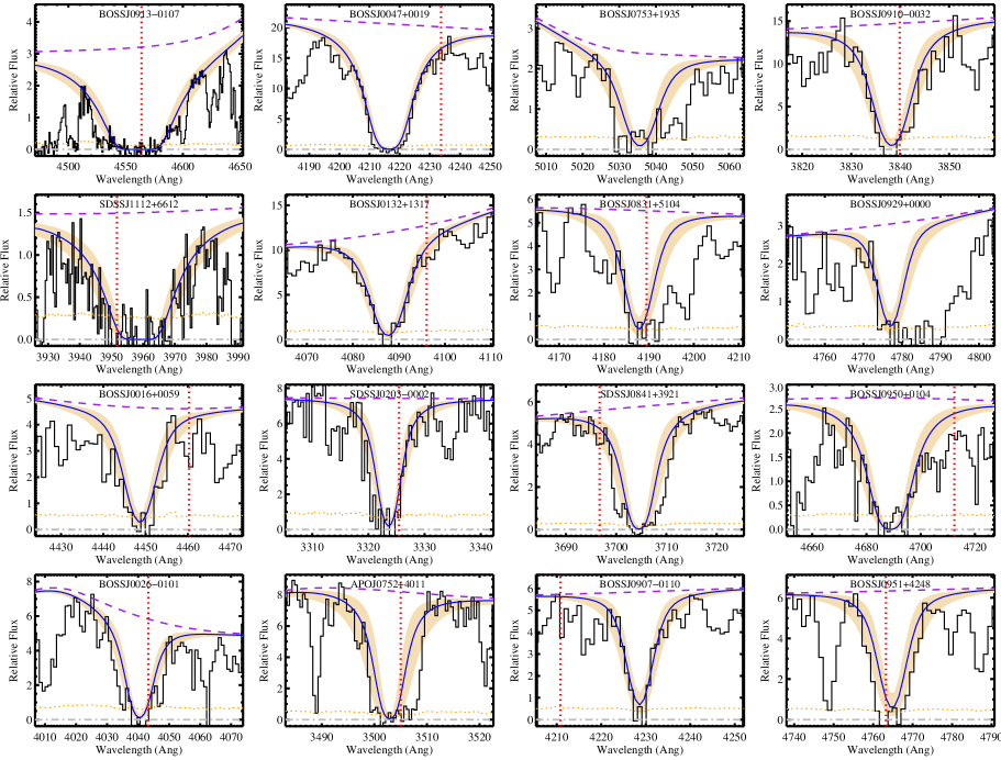
Figure 24.— Voigt profile models for the strongest H I absorbers in the QPQ6 dataset (solid blue curves with shaded regions showing the error estimate; Table 4). The purple dotted lines trace our estimate of the quasar continuum, the red dotted line marks Ly$\alpha$ of the f/g quasar ($\lambda_{\rm Ly\alpha}^{\rm fg}$), and the dotted curve traces the error array.

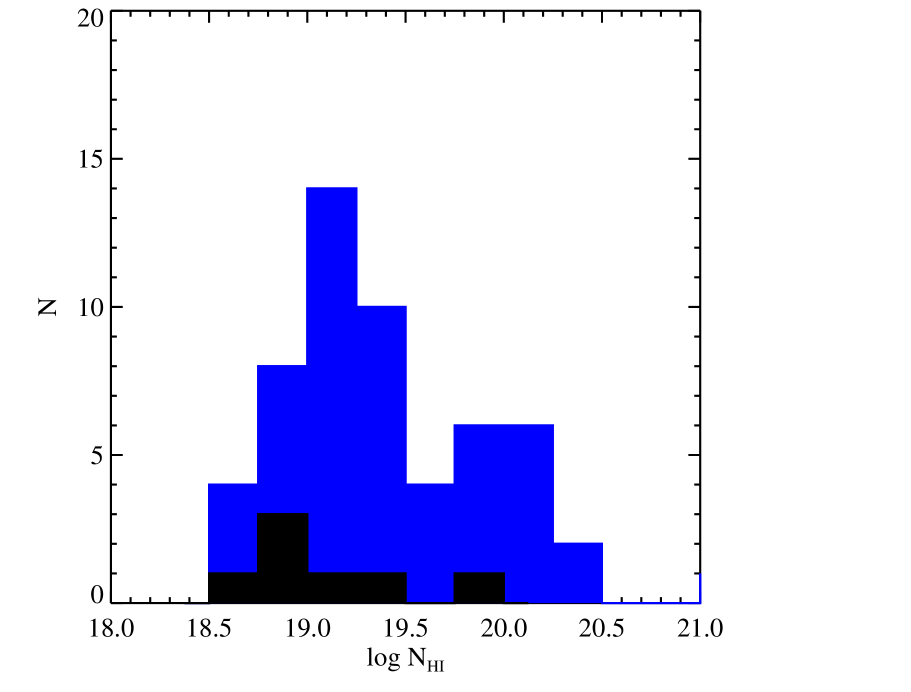
Figure 25.— Distribution of measured $N_{\rm HI}$ values along the line of sight towards quasar pairs (blue) compared to the distribution from our control sample (black). We find the shape of the two distributions are similar. The cutoff at $N_{\rm HI}\approx 10^{19}\,{\rm cm^{-2}}$ follows from our sensitivity to damping wings in the Ly$\alpha$ transition.

References

- Abazajian et al. (2009) Abazajian, K. N., et al. 2009, ApJS, 182, 543
- Adelberger et al. (2005a) Adelberger, K. L., Shapley, A. E., Steidel, C. C., Pettini, M., Erb, D. K., & Reddy, N. A. 2005a, ApJ, 629, 636
- Adelberger et al. (2005b) Adelberger, K. L., Steidel, C. C., Pettini, M., Shapley, A. E., Reddy, N. A., & Erb, D. K. 2005b, ApJ, 619, 697
- Adelberger et al. (2003) Adelberger, K. L., Steidel, C. C., Shapley, A. E., & Pettini, M. 2003, ApJ, 584, 45
- Ahn et al. (2012) Ahn, C. P., et al. 2012, ApJS, 203, 21
- Altay et al. (2011) Altay, G., Theuns, T., Schaye, J., Crighton, N. H. M., & Dalla Vecchia, C. 2011, ApJ, 737, L37
- Antonucci (1993) Antonucci, R. 1993, ARA&A, 31, 473
- Bajtlik et al. (1988) Bajtlik, S., Duncan, R. C., & Ostriker, J. P. 1988, ApJ, 327, 570
- Bardeen et al. (1986) Bardeen, J. M., Bond, J. R., Kaiser, N., & Szalay, A. S. 1986, ApJ, 304, 15
- Barkana (2004) Barkana, R. 2004, MNRAS, 347, 59
- Behroozi et al. (2013) Behroozi, P. S., Wechsler, R. H., Wu, H.-Y., Busha, M. T., Klypin, A. A., & Primack, J. R. 2013, ApJ, 763, 18
- Bernstein et al. (2003) Bernstein, R., Shectman, S. A., Gunnels, S. M., Mochnacki, S., & Athey, A. E. 2003, in Instrument Design and Performance for Optical/Infrared Ground-based Telescopes. Edited by Iye, Masanori; Moorwood, Alan F. M. Proceedings of the SPIE, Volume 4841, pp. 1694-1704 (2003)., 1694–1704
- Bielby et al. (2013) Bielby, R., et al. 2013, MNRAS, 430, 425
- Bielby et al. (2011) Bielby, R. M., et al. 2011, MNRAS, 414, 2
- Bochanski et al. (2009) Bochanski, J. J., et al. 2009, PASP, 121, 1409
- Bouché & Lowenthal (2004) Bouché, N., & Lowenthal, J. D. 2004, ApJ, 609, 513
- Bouché et al. (2004) Bouché, N., Murphy, M. T., & Péroux, C. 2004, MNRAS, 354, L25
- Bovy et al. (2011) Bovy, J., et al. 2011, ApJ, 729, 141
- Bovy et al. (2012) —. 2012, ApJ, 749, 41
- Bowen et al. (2006) Bowen, D. V., et al. 2006, ApJ, 645, L105
- Brooks et al. (2009) Brooks, A. M., Governato, F., Quinn, T., Brook, C. B., & Wadsley, J. 2009, ApJ, 694, 396
- Cantalupo et al. (2012) Cantalupo, S., Lilly, S. J., & Haehnelt, M. G. 2012, MNRAS, 425, 1992
- Cantalupo & Porciani (2011) Cantalupo, S., & Porciani, C. 2011, MNRAS, 411, 1678
- Chelouche et al. (2008) Chelouche, D., Ménard, B., Bowen, D. V., & Gnat, O. 2008, ApJ, 683, 55
- Chen et al. (2005) Chen, H.-W., Prochaska, J. X., Weiner, B. J., Mulchaey, J. S., & Williger, G. M. 2005, ApJ, 629, L25
- Conroy et al. (2008) Conroy, C., Shapley, A. E., Tinker, J. L., Santos, M. R., & Lemson, G. 2008, ApJ, 679, 1192
- Cooke et al. (2006a) Cooke, J., Wolfe, A. M., Gawiser, E., & Prochaska, J. X. 2006a, ApJ, 636, L9
- Cooke et al. (2006b) —. 2006b, ApJ, 652, 994
- Cooksey et al. (2013) Cooksey, K. L., Kao, M. M., Simcoe, R. A., O’Meara, J. M., & Prochaska, J. X. 2013, ApJ, 763, 37
- Crighton et al. (2011) Crighton, N. H. M., et al. 2011, MNRAS, 414, 28
- Croft (2004) Croft, R. A. C. 2004, ApJ, 610, 642
- Croom et al. (2005) Croom, S. M., et al. 2005, MNRAS, 356, 415
- Croom et al. (2004) Croom, S. M., Smith, R. J., Boyle, B. J., Shanks, T., Miller, L., Outram, P. J., & Loaring, N. S. 2004, MNRAS, 349, 1397
- Dall’Aglio et al. (2008) Dall’Aglio, A., Wisotzki, L., & Worseck, G. 2008, A&A, 491, 465
- Dekel & Birnboim (2006) Dekel, A., & Birnboim, Y. 2006, MNRAS, 368, 2
- Dekel et al. (2009) Dekel, A., et al. 2009, Nature, 457, 451
- Dessauges-Zavadsky et al. (2009) Dessauges-Zavadsky, M., Ellison, S. L., & Murphy, M. T. 2009, MNRAS, 396, L61
- Ellison et al. (2007) Ellison, S. L., Hennawi, J. F., Martin, C. L., & Sommer-Larsen, J. 2007, MNRAS, 378, 801
- Elvis (2000) Elvis, M. 2000, ApJ, 545, 63
- Erkal et al. (2012) Erkal, D., Gnedin, N. Y., & Kravtsov, A. V. 2012, ApJ, 761, 54
- Farina et al. (2013) Farina, E. P., Falomo, R., Decarli, R., Treves, A., & Kotilainen, J. K. 2013, MNRAS, 429, 1267
- Faucher-Giguère & Kereš (2011) Faucher-Giguère, C.-A., & Kereš, D. 2011, MNRAS, 412, L118
- Faucher-Giguère et al. (2008a) Faucher-Giguère, C.-A., Lidz, A., Hernquist, L., & Zaldarriaga, M. 2008a, ApJ, 688, 85
- Faucher-Giguère et al. (2008b) Faucher-Giguère, C.-A., Lidz, A., Zaldarriaga, M., & Hernquist, L. 2008b, ApJ, 673, 39
- Faucher-Giguère et al. (2008c) Faucher-Giguère, C.-A., Prochaska, J. X., Lidz, A., Hernquist, L., & Zaldarriaga, M. 2008c, ApJ, 681, 831
- Font-Ribera et al. (2013) Font-Ribera, A., et al. 2013, JCAP, 5, 18
- Font-Ribera et al. (2012) —. 2012, JCAP, 11, 59
- Fumagalli et al. (2013a) Fumagalli, M., Hennawi, J. F., Prochaska, J. X., Kasen, D., Dekel, A., Ceverino, D., & Primack, J. 2013a, ArXiv e-prints
- Fumagalli et al. (2011a) Fumagalli, M., O’Meara, J. M., & Prochaska, J. X. 2011a, Science, 334, 1245
- Fumagalli et al. (2013b) Fumagalli, M., O’Meara, J. M., Prochaska, J. X., & Worseck, G. 2013b, ArXiv e-prints
- Fumagalli et al. (2011b) Fumagalli, M., Prochaska, J. X., Kasen, D., Dekel, A., Ceverino, D., & Primack, J. R. 2011b, MNRAS, 418, 1796
- Gaskell (2009) Gaskell, C. M. 2009, NAR, 53, 140
- Gnedin & Hollon (2012) Gnedin, N. Y., & Hollon, N. 2012, ApJS, 202, 13
- Gnedin & Hui (1998) Gnedin, N. Y., & Hui, L. 1998, MNRAS, 296, 44
- Hennawi (2004) Hennawi, J. F. 2004, Ph.D. Thesis
- Hennawi et al. (2010) Hennawi, J. F., et al. 2010, ApJ, 719, 1672
- Hennawi & Prochaska (2007) Hennawi, J. F., & Prochaska, J. X. 2007, ApJ, 655, 735
- Hennawi & Prochaska (2013) —. 2013, ApJ, 766, 58 (QPQ4)
- Hennawi et al. (2006a) Hennawi, J. F., et al. 2006a, ApJ, 651, 61
- Hennawi et al. (2006b) —. 2006b, AJ, 131, 1
- Hewett & Wild (2010) Hewett, P. C., & Wild, V. 2010, MNRAS, 405, 2302
- Hook et al. (2004) Hook, I. M., Jørgensen, I., Allington-Smith, J. R., Davies, R. L., Metcalfe, N., Murowinski, R. G., & Crampton, D. 2004, PASP, 116, 425
- Hui (1999) Hui, L. 1999, ApJ, 516, 519
- Kaplan et al. (2010) Kaplan, K. F., Prochaska, J. X., Herbert-Fort, S., Ellison, S. L., & Dessauges-Zavadsky, M. 2010, PASP, 122, 619
- Kereš et al. (2009) Kereš, D., Katz, N., Davé, R., Fardal, M., & Weinberg, D. H. 2009, MNRAS, 396, 2332
- Kereš et al. (2005) Kereš, D., Katz, N., Weinberg, D. H., & Davé, R. 2005, MNRAS, 363, 2
- Kim & Croft (2008) Kim, Y.-R., & Croft, R. A. C. 2008, MNRAS, 387, 377
- Kirkman & Tytler (2008) Kirkman, D., & Tytler, D. 2008, MNRAS, 391, 1457
- Kulkarni et al. (2010) Kulkarni, V. P., Khare, P., Som, D., Meiring, J., York, D. G., Péroux, C., & Lauroesch, J. T. 2010, Nature, 15, 735
- Lee et al. (2013) Lee, K.-G., et al. 2013, AJ, 145, 69
- Lee et al. (2012) Lee, K.-G., Suzuki, N., & Spergel, D. N. 2012, AJ, 143, 51
- Lee et al. (2011) Lee, T. S., Nagamine, K., Hernquist, L., & Springel, V. 2011, MNRAS, 411, 54
- Maller & Bullock (2004) Maller, A. H., & Bullock, J. S. 2004, MNRAS, 355, 694
- Maller et al. (2001) Maller, A. H., Prochaska, J. X., Somerville, R. S., & Primack, J. R. 2001, MNRAS, 326, 1475
- Marshall et al. (2008) Marshall, J. L., et al. 2008, in Society of Photo-Optical Instrumentation Engineers (SPIE) Conference Series, Vol. 7014, Society of Photo-Optical Instrumentation Engineers (SPIE) Conference Series
- Martin et al. (2010) Martin, C. L., Scannapieco, E., Ellison, S. L., Hennawi, J. F., Djorgovski, S. G., & Fournier, A. P. 2010, ApJ, 721, 174
- Martin et al. (2012) Martin, C. L., Shapley, A. E., Coil, A. L., Kornei, K. A., Bundy, K., Weiner, B. J., Noeske, K. G., & Schiminovich, D. 2012, ApJ, 760, 127
- McDonald & Miralda-Escudé (1999) McDonald, P., & Miralda-Escudé, J. 1999, ApJ, 519, 486
- McLure & Dunlop (2004) McLure, R. J., & Dunlop, J. S. 2004, MNRAS, 352, 1390
- McQuinn et al. (2011) McQuinn, M., Oh, S. P., & Faucher-Giguère, C.-A. 2011, ApJ, 743, 82
- Miralda-Escudé et al. (1996) Miralda-Escudé, J., Cen, R., Ostriker, J. P., & Rauch, M. 1996, ApJ, 471, 582
- Mo & Miralda-Escude (1996) Mo, H. J., & Miralda-Escude, J. 1996, ApJ, 469, 589
- Moe et al. (2009) Moe, M., Arav, N., Bautista, M. A., & Korista, K. T. 2009, ApJ, 706, 525
- Myers et al. (2007) Myers, A. D., Brunner, R. J., Richards, G. T., Nichol, R. C., Schneider, D. P., & Bahcall, N. A. 2007, ApJ, 658, 99
- Nestor et al. (2005) Nestor, D. B., Turnshek, D. A., & Rao, S. M. 2005, ApJ, 628, 637
- Noterdaeme et al. (2012) Noterdaeme, P., et al. 2012, A&A, 547, L1
- Oke et al. (1995) Oke, J. B., et al. 1995, PASP, 107, 375
- O’Meara et al. (2007) O’Meara, J. M., Prochaska, J. X., Burles, S., Prochter, G., Bernstein, R. A., & Burgess, K. M. 2007, ApJ, 656, 666
- O’Meara et al. (2011) O’Meara, J. M., Prochaska, J. X., Chen, H.-W., & Madau, P. 2011, ApJS, 195, 16
- O’Meara et al. (2013) O’Meara, J. M., Prochaska, J. X., Worseck, G., Chen, H.-W., & Madau, P. 2013, ApJ, 765, 137
- Oppenheimer & Schaye (2013) Oppenheimer, B. D., & Schaye, J. 2013, ArXiv e-prints
- Padilla et al. (2009) Padilla, N., Lacerna, I., Lopez, S., Barrientos, L. F., Lira, P., Andrews, H., & Tejos, N. 2009, MNRAS, 395, 1135
- Pâris et al. (2012) Pâris, I., et al. 2012, A&A, 548, A66
- Péroux et al. (2007) Péroux, C., Dessauges-Zavadsky, M., D’Odorico, S., Kim, T.-S., & McMahon, R. G. 2007, MNRAS, 382, 177
- Péroux et al. (2005) Péroux, C., Dessauges-Zavadsky, M., D’Odorico, S., Sun Kim, T., & McMahon, R. G. 2005, MNRAS, 363, 479
- Péroux et al. (2006) Péroux, C., Kulkarni, V. P., Meiring, J., Ferlet, R., Khare, P., Lauroesch, J. T., Vladilo, G., & York, D. G. 2006, A&A, 450, 53
- Pogge et al. (2012) Pogge, R. W., et al. 2012, in Society of Photo-Optical Instrumentation Engineers (SPIE) Conference Series, Vol. 8446, Society of Photo-Optical Instrumentation Engineers (SPIE) Conference Series
- Pontzen et al. (2008) Pontzen, A., et al. 2008, MNRAS, 390, 1349
- Porciani et al. (2004) Porciani, C., Magliocchetti, M., & Norberg, P. 2004, MNRAS, 355, 1010
- Prochaska & Hennawi (2009) Prochaska, J. X., & Hennawi, J. F. 2009, ApJ, 690, 1558
- Prochaska et al. (2008) Prochaska, J. X., Hennawi, J. F., & Herbert-Fort, S. 2008, ApJ, 675, 1002
- Prochaska et al. (2013) Prochaska, J. X., Hennawi, J. F., & Simcoe, R. A. 2013, ApJ, 762, L19 (QPQ5)
- Prochaska et al. (2005) Prochaska, J. X., Herbert-Fort, S., & Wolfe, A. M. 2005, ApJ, 635, 123
- Prochaska et al. (2006) Prochaska, J. X., O’Meara, J. M., Herbert-Fort, S., Burles, S., Prochter, G. E., & Bernstein, R. A. 2006, ApJ, 648, L97
- Prochaska et al. (2010) Prochaska, J. X., O’Meara, J. M., & Worseck, G. 2010, ApJ, 718, 392
- Prochaska et al. (2011) Prochaska, J. X., Weiner, B., Chen, H.-W., Mulchaey, J., & Cooksey, K. 2011, ApJ, 740, 91
- Prochaska & Wolfe (2009) Prochaska, J. X., & Wolfe, A. M. 2009, ApJ, 696, 1543
- Prochaska et al. (2001) Prochaska, J. X., et al. 2001, ApJS, 137, 21
- Rafelski et al. (2012) Rafelski, M., Wolfe, A. M., Prochaska, J. X., Neeleman, M., & Mendez, A. J. 2012, ApJ, 755, 89
- Rahmati et al. (2013) Rahmati, A., Pawlik, A. H., Raicevic, M., & Schaye, J. 2013, MNRAS, 430, 2427
- Rakic et al. (2012) Rakic, O., Schaye, J., Steidel, C. C., & Rudie, G. C. 2012, ApJ, 751, 94
- Ribaudo et al. (2011) Ribaudo, J., Lehner, N., & Howk, J. C. 2011, ApJ, 736, 42
- Richards et al. (2002) Richards, G. T., Vanden Berk, D. E., Reichard, T. A., Hall, P. B., Schneider, D. P., SubbaRao, M., Thakar, A. R., & York, D. G. 2002, AJ, 124, 1
- Rorai et al. (2013) Rorai, A., Hennawi, J. F., & White, M. 2013, ArXiv e-prints
- Rosario et al. (2013) Rosario, D. J., et al. 2013, ArXiv e-prints
- Rubin et al. (2013) Rubin, K. H. R., Prochaska, J. X., Koo, D. C., Phillips, A. C., Martin, C. L., & Winstrom, L. O. 2013, ArXiv e-prints
- Rudie et al. (2012) Rudie, G. C., et al. 2012, ApJ, 750, 67
- Rupke et al. (2005) Rupke, D. S., Veilleux, S., & Sanders, D. B. 2005, ApJS, 160, 115
- Santini et al. (2012) Santini, P., et al. 2012, A&A, 540, A109
- Schaye (2006) Schaye, J. 2006, ApJ, 643, 59
- Schaye et al. (2007) Schaye, J., Carswell, R. F., & Kim, T.-S. 2007, MNRAS, 379, 1169
- Schneider et al. (2010) Schneider, D. P., et al. 2010, AJ, 139, 2360
- Scott et al. (2000) Scott, J., Bechtold, J., Dobrzycki, A., & Kulkarni, V. P. 2000, ApJS, 130, 67
- Shapley et al. (2003) Shapley, A. E., Steidel, C. C., Pettini, M., & Adelberger, K. L. 2003, ApJ, 588, 65
- Sheinis et al. (2002) Sheinis, A. I., Bolte, M., Epps, H. W., Kibrick, R. I., Miller, J. S., Radovan, M. V., Bigelow, B. C., & Sutin, B. M. 2002, PASP, 114, 851
- Shen et al. (2013) Shen, S., Madau, P., Guedes, J., Mayer, L., Prochaska, J. X., & Wadsley, J. 2013, ApJ, 765, 89
- Shen (2009) Shen, Y. 2009, ApJ, 704, 89
- Shen et al. (2010) Shen, Y., et al. 2010, ApJ, 719, 1693
- Shen et al. (2011) —. 2011, ApJS, 194, 45
- Shen et al. (2007) —. 2007, AJ, 133, 2222
- Simcoe et al. (2002) Simcoe, R. A., Sargent, W. L. W., & Rauch, M. 2002, ApJ, 578, 737
- Steidel et al. (2010) Steidel, C. C., Erb, D. K., Shapley, A. E., Pettini, M., Reddy, N., Bogosavljević, M., Rudie, G. C., & Rakic, O. 2010, ApJ, 717, 289
- Steidel et al. (1996) Steidel, C. C., Giavalisco, M., Pettini, M., Dickinson, M., & Adelberger, K. L. 1996, ApJ, 462, L17+
- Stewart et al. (2011) Stewart, K. R., Kaufmann, T., Bullock, J. S., Barton, E. J., Maller, A. H., Diemand, J., & Wadsley, J. 2011, ApJ, 735, L1
- Tejos et al. (2012) Tejos, N., Morris, S. L., Crighton, N. H. M., Theuns, T., Altay, G., & Finn, C. W. 2012, MNRAS, 425, 245
- Teyssier (2002) Teyssier, R. 2002, A&A, 385, 337
- Tinker & Chen (2008) Tinker, J. L., & Chen, H.-W. 2008, ApJ, 679, 1218
- Trainor & Steidel (2012) Trainor, R. F., & Steidel, C. C. 2012, ApJ, 752, 39
- Tumlinson et al. (2013) Tumlinson, J., Thom, C., Werk, J. K., & J.X., P. 2013, ApJ, submitted
- van de Voort & Schaye (2012) van de Voort, F., & Schaye, J. 2012, MNRAS, 423, 2991
- Vogt et al. (1994) Vogt, S. S., et al. 1994, in Proc. SPIE Instrumentation in Astronomy VIII, David L. Crawford; Eric R. Craine; Eds., Volume 2198, p. 362, 362–+
- Weiner et al. (2009) Weiner, B. J., et al. 2009, ApJ, 692, 187
- White et al. (2012) White, M., et al. 2012, MNRAS, 424, 933
- Wild et al. (2008) Wild, V., et al. 2008, MNRAS, 388, 227
- Wolfe et al. (2005) Wolfe, A. M., Gawiser, E., & Prochaska, J. X. 2005, ARA&A, 43, 861