Data Driven Search in the Displaced $b\bar{b}$ Pair Channel for a Higgs Boson Decaying to Long-Lived Neutral Particles

Abstract:

This article presents a proposal for a new search channel for the Higgs boson decaying to two long-lived neutral particles, each of which decays to $b\bar{b}$ at a displaced vertex. The decay length considered is such that the decay takes place within the LHC beampipe. We present a new data-driven analysis using jet substructure and properties of the tracks from the highly-displaced vertices. We consider a model with a 125 GeV Higgs boson with a significant branching fraction to decay via this mode, with the long-lived neutral particle having a mass in the range of 15–40 GeV and a decay length commensurate with the beam pipe radius. Such a signal can be readily observed with an integrated luminosity of 19.5 fb^-1 at 8 TeV at the LHC.

1 Introduction

Until recently, the Higgs sector was one of the great unknowns in our current understanding of particle physics, and the primary target of the current Tevatron and Large Hadron Collider (LHC) programs. The new scalar boson recently discovered at the LHC by the ATLAS and CMS experiments [1, 2] has, so far, been measured to be consistent with a Standard Model (SM) Higgs boson [3, 4]. However, the systematic uncertainties in the measurements still allow for the possibility that this new particle could be responsible for electroweak symmetry breaking and mass generation but not be the SM Higgs boson. In particular, it could have non-SM properties such as mixing with a singlet, non-standard couplings to the fermions, or other exotic decays. If one assumes a Higgs with SM couplings except additional decay channel to new particles, a branching ratio as large as 20% can be accommodated given the 2012 LHC data [5, 6].

In this article we address an exotic Higgs decay mode that would have escaped existing search strategies. We consider the possibility [7] (see also [8, 9] for closely related work) that the Higgs boson $h$ decays to two spin-zero neutral particles $X$, and the $X$ decays in turn to $b\bar{b}$ with a displaced vertex. More specifically, we will consider the case where the lifetime $\tau_{X}$ of the $X$ puts its decay at a distance from the collision point of order millimeters to a few centimeters, so that the decay vertex remains within the LHC beampipe. Searches for related signatures have also been made in D0 and ATLAS. In D0, the typical decay to two $b\bar{b}$ pairs in the several to 20 centimeter range has been studied and weakly constrained [10]. In ATLAS, strong limits on final states with a muon and multiple displaced jets have been obtained [11]; however, as the model considered involves an $R$-parity-violating neutralino decay into a muon and hadrons, the transverse momentum of the muon was required to be higher than 50 GeV/$c$, which is unlikely to result from the semileptonic decay of the bottom quark used in our model.

It is sometimes argued that searches of this type are not so well-motivated, because the chance of the $X$ having a lifetime that allows for decays inside the detector is low. However, there are both theoretical and experimental considerations in favor. First, long-lived particles are less rare in models  [13, 12, 8, 7, 9, 14, 15, 16, 17, 18, 19, 20, 21] than is commonly assumed. In hidden valley models ([22], for instance), there may be not one but many new particle states with a wide variety of lifetimes, similar to the case of QCD, and this plenitude makes it more likely that one of these particles will have a detectable displaced decay. Second, decays of such particles have such limited SM background that in principle only a few such events might suffice for a discovery, so even a small branching fraction for such particles may lead to a discovery opportunity. That said, detector backgrounds can be a serious issue, and event triggering and reconstruction may be an even larger one if the lifetimes are long enough. Each search strategy has its own features, and some are easier than others.

The Tevatron and LHC detectors were generally not optimized for finding long-lived particles, with the exception of $B$ hadrons, and searches for such particles face numerous challenges. In this paper we consider the case that, relatively speaking, is the easiest: a search for a new particle that mainly decays before that particle reaches the beampipe. Such decays face little or no background from secondary interactions of hadrons with detector material, and the dominant background is a physics background from real $B$ hadron decays. However, to the extent the $X$ lives longer than the $B$ hadron and is considerably heavier, distinguishing it from SM heavy-flavor backgrounds should be easier. For the specific case of $h\to XX$, the situation is better still, since there are two $X$ decays per event, and also a mass resonance that may be reconstructable.

The main purpose of our paper is to suggest a search strategy for $h\to XX$, with $X$ decaying to $b\bar{b}$ before passing through the wall of the beampipe. These events are selected online with a trigger requiring a single muon and two $b$-jets tagged using an algorithm measuring the secondary vertex displacement. When the mass of the $X$ is heavy, the resulting $b$-jets typically have low $p_{T}$ and cannot be triggered efficiently. Hence, we focus on the region where $X$ is light and so the jets from the two $b$-quarks merge into a single reconstructed jet. Also, as we will describe in this paper, by merging two $b$-quarks into one jet, the QCD background can be estimated using data-driven methods. Data-driven techqniues are crucial for low mass signals, where systematic uncertainty can be very large. To extract the signal, we then select $X$ boson candidates by looking for jets meeting a combination of two requirements: first, using the displacement of the individual tracks to identify long-lived particles, and second, using the internal substructure of the jet to further distinguish exotic displaced jets from displaced $b$-jets. By combining jet substructure with displaced tracks and vertices, it is possible to devise a new exotic jet tagger and propose a data-driven method for estimating the QCD background. Using our technique, it is demonstrated that new long-lived neutral particles originating from a 125 GeV/$c^{2}$ Higgs boson may be discovered using 19.5 fb^-1 of LHC data recorded at $\sqrt{s}=8$ TeV.

For our studies, we focus on a model with a non-SM Higgs with a mass of 125 GeV/$c^{2}$, which then decays into a pair of long-lived neutral bosons $X$ whose mass ranges from 15 to 40 GeV/$c^{2}$. For the boson $X$, we primarily consider the case where the $X$ subsequently decays into $b\bar{b}$. Because of the relatively low mass of the $X$ bosons considered, the $b\bar{b}$ pair is generally reconstructed as a single jet in the detector. We use the anti-$k_{T}$ [23] algorithm with $\Delta R=1.0$ in this analysis to capture the hadrons from both $b$ quarks in a single object, which we refer to as a “fat jet”. The final topology consists of two fat jets producing a resonance at the expected Higgs mass, with a distinctive two-prong jet substructure in each jet. The predominant background is the QCD production of $b\bar{b}$ pairs. However, since these pairs are being produced from a single quark, they will tend to have fewer displaced tracks, and will tend to contain only one central hard prong. These properties allow us to differentiate the signal from the much larger background.

The need for using large-radius jets instead of the standard cone size of $\Delta R=0.5$ is illustrated in Figure 1. This figure shows the results of jet reconstruction in a simulated signal sample with $m_{H}=125$ GeV/$c^{2}$, $m_{X}=20$ GeV/$c^{2}$, and $c\tau=2$ mm for two different cone sizes: the standard cone size of $\Delta R=0.5$, and our enlarged cone size of $\Delta R=1.0$. In Figure 1, we see that even with the standard cone size, in the vast majority of events the $X\rightarrow b\bar{b}$ decay is reconstructed as a single merged jet, rather than two separate jets. However, Figure 1 shows that the standard cone size is too small to capture all of the radiation from this merged jet, resulting in a significant underestimation of the reconstructed mass. Using a larger cone radius thus offers two advantages: first, the event is nearly always reconstructed with exactly two jets, allowing for more predictable reconstruction; and second, the cone size is large enough to capture all of the merged jet, allowing for more accurate mass reconstruction. We can then use subjet techniques on the merged jets to identify the two constituents.

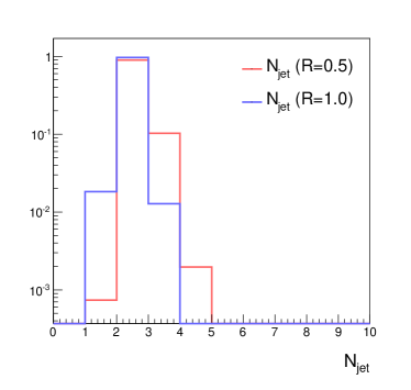
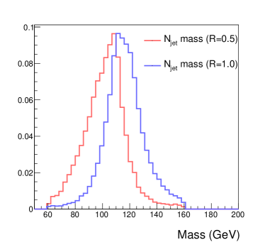
Figure 1: Results of jet clustering in simulated signal samples. Left: number of reconstructed jets using the standard cone radius of $\Delta R=0.5$ (red) and our cone radius of $\Delta R=1.0$ (blue). Right: Reconstructed two-jet mass for these two different cone radii. The signal model shown is with $m_{H}=125$ GeV/$c^{2}$, $m_{X}=20$ GeV/$c^{2}$, and $c\tau=2$ mm.

In this article a variety of proper lifetimes $c\tau$ for the long-lived particle ranging from 1 mm to 10 mm was considered. At very low lifetimes, the displacements of the resulting tracks and vertices become too small to consistently separate the signal events from background, while at high lifetimes the track and muon reconstructions suffer from inefficiencies in the tracking and trigger algorithms, which are not generally designed for highly-displaced particles. However, our simple detector simulation will be unable to take these effects into account and hence we refrain from extending our results beyond 30 mm.

Although our search strategy uses $h\to XX$ as a benchmark for optimization, it is not strongly dependent on the specific initial or final state. Consequently it should be somewhat model-independent, and would be sensitive to a variety of models with two long-lived particles in the events. For example, certain gauge-mediated supersymmetric models with a neutralino [24] decaying in flight to a $Z$ or $h$ might be picked up by our search. One point of model-dependence worth keeping in mind is that the heavy-flavor content of the $X$ decay is important for our strategy, as we will base our study on a $b$-tagger-like trigger.

2 Event Generation

At hadron colliders the dominant Higgs production mechanism is via gluon-gluon fusion. In this note we study the process $gg\rightarrow h\rightarrow(X\rightarrow b\bar{b})(X\rightarrow b\bar{b})$, where the Higgs boson is produced by gluon fusion and then decays into a pair of long lived (pseudo-)scalars which then each decay to a pair of bottom quarks. We consider this in the context of $pp$ collisions at a center-of-mass energy of $8$ TeV.

We generate the signal samples for Higgs mass $m_{h}=$ 125 GeV/$c^{2}$ and the (pseudo-)scalar mass $m_{X}$ between 15 and 40 GeV/$c^{2}$ with 5 GeV/$c^{2}$ steps. Samples were generated for the $c\tau_{X}$ of the scalar varying within a wide range between 0.1 mm to 30 mm. The signal sample is generated using Pythia 6.4.27 [25]. For the production cross section, we use the NLO cross section for SM $gg\rightarrow h$ production, which is 19.3 pb at 8 TeV [26].

The dominant background for this process comes from QCD heavy quark production, particularly events with one or more $b\bar{b}$ pairs, which represents the most difficult background to remove. Using MadGraph 5 v1.5.7 [27], we generated a sample of 500 million $b\bar{b}$ events matched up to four jets (including $b\bar{b}b\bar{b}$ and $b\bar{b}c\bar{c}$), and showered them through Pythia [25]. Matching is done using the MLM prescription [28]. In order to account for effects that may not be fully modeled in the simulation, a K-factor of 1.6 is obtained by generating another QCD $b\bar{b}$ sample at 7 TeV and reproducing the CMS analysis published in [29] (see Appendix A for details and discussion on effects from fake $b$-tags). We used the CTEQ6L1 PDF for both the signal and the background [30].

To simulate particle flow jets at CMS, the stable particles (except neutrinos) are clustered into large anti-$k_{T}$ [23] jets with a cone size of $\Delta R=1.0$ using FastJet 3.0.2 [32]. Because our jets use an anti-$k_{T}$ algorithm with a large cone size to capture as much of the $b\bar{b}$ decay as possible, they are more susceptible to underlying event and pileup effects. In order to overcome these issues, we use jet trimming with $R_{\textrm{trim}}=0.3$ and $f_{\textrm{cut}}=0.05$ [38]. The resulting jets are then smeared using the momentum resolution given in [33] . To simulate the detector response in the tracker, we associate a track to each charged final state particle with $p_{T}>1$ GeV/$c$. The production vertex of the track is then smeared by an uncertainty $\sigma_{\textrm{trk}}$, extracted from [31]:

$$\sigma_{\textrm{trk}} =a+\frac{b}{p_{T}}+\left(c+\frac{d}{p_{T}}\right)\eta^{2}$$ (1)

$$a=20.4\quad b= 56.4\quad c=-0.11\quad d=18.2,$$

where $\sigma_{\textrm{trk}}$ is in units of $\mu$m and $p_{T}$ in units of GeV/$c$. To avoid complications in finding the vertex location of our event along the beamline, we do not use any tracking information in the longitudinal direction. The QCD background is validated against published CMS results. For details, see Appendix A.

3 Displaced Jet Variables

In the following, we discuss the key variables used for identifying long-lived decays. We postpone the discussion on event selection until Section 5, where all the analysis strategies and cuts are listed in detail.

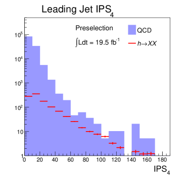
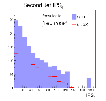
Figure 2: Distributions of $\textrm{IPS}_{4}$ after preselection. The QCD background is given by the matched $b\bar{b}$ sample, and the signal model shown is with $m_{H}=125$ GeV/$c^{2}$, $m_{X}=20$ GeV/$c^{2}$, and $c\tau=2$ mm. The signal is assumed to have SM gluon fusion production with 100% branching ratio to $XX$. Left: for the leading jet. Right: for the second-leading jet.

The primary tool we use to measure the displacement of a jet is to examine the displacement of the individual tracks in the jet. For each track, we compute the transverse Impact Parameter (IP) as follows:

$$\textrm{IP}=\frac{|v_{x}\cdot p_{y}-v_{y}\cdot p_{x}|}{p_{T}}$$ (2)

The computed IP has an associated error $\sigma_{\textrm{IP}}^{2}=\sigma^{2}_{\textrm{trk}}+\sigma^{2}_{\textrm{PV}}$, where $\sigma_{\textrm{trk}}$ is given by equation 1, and $\sigma_{\textrm{PV}}=0.025\,\mu\textrm{m}$ is the uncertainty associated with the transverse coordinate of the Primary Vertex (PV), as determined in [31]. In an actual detector, the track IP errors are often as large as the measured track IP itself, and it is advantageous to consider the impact parameter significance (IPS) [35]

$$\textrm{IPS}=\frac{\textrm{IP}}{\sigma_{\textrm{IP}}}$$ (3)

For prompt tracks, the IPS distribution tends to have a strong peak around zero and the spread of the distribution depends on the mismeasurement of the IPS or misalignment. For genuine displaced tracks, the IPS distribution will tend to have a significant tail. Validation of the IPS variable against published data is presented in Appendix A.

For each jet, we order the associated tracks in decreasing IPS. We then consider the fourth-highest IPS value, denoted by $\textrm{IPS}_{4}$. A typical $b$-jet will tend to only have two displaced tracks, while a displaced $b\bar{b}$ pair will have four, so this variable is expected to have significant discriminating power. Figure 2 shows the $\textrm{IPS}_{4}$ distributions for signal vs. QCD.

Other variables, such the significance of the decay length of the jet vertex and the fraction of the jet energy carried by prompt tracks, were considered as discriminants for identifying displaced particle decays. However, they did not result in a significant increase in discriminating power, so due to the lack of validation of these other variables and for the sake of simplicity, we do not use these in our analysis.

4 Jet Substructure

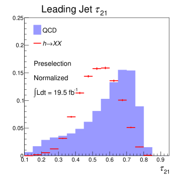
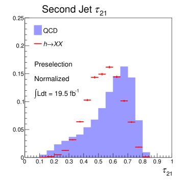
Figure 3: Distribution of $\tau_{21}$ for the leading jet (left) and the second-leading jet (right) for simulated signal events and $b\bar{b}$ background, for a signal model with $m_{H}=125$ GeV/$c^{2}$ and $m_{X}=20$ GeV/$c^{2}$.

In this analysis we look for “fat jets” that originate from the decay of the long-lived particle into a $b\bar{b}$ pair, and we expect the “fat jet” to contain a different substructure than jets originating from a single $b$ quark. In order to quantify this substructure, we use the “$N$-subjettiness” variables defined in [36, 37]. Briefly, one first defines $\tau_{N}$ by fitting $N$ axes to a jet, and computing

$$\tau_{N}=\frac{1}{d_{0}}\sum_{k}p_{T,k}\min\{\Delta R_{1,k},\ldots\Delta R_{N,k}\},$$ (4)

where $k$ runs over the constituents in the jet and $d_{0}$ is an unimportant overall normalization factor. $\tau_{N}$ is then minimized over all possible choices of the $N$ subjet axes. $\tau_{N}$ thus shows to what degree the jet can be viewed as being composed of $N$ individual subjets. For distinguishing jets with two subjets from one, we use $\tau_{21}=\tau_{2}/\tau_{1}$. If $\tau_{21}$ is close to 0, that indicates that the jet is strongly favored to have two subjets, as we would expect from our signal jets, while a $\tau_{21}$ close to 1 indicates that the jet does not have a two-subjet structure, as we would expect from QCD. One can see from Figure 3 that the $\tau_{21}$ distributions are indeed different between signal and QCD.

5 Event Selection

Following the definition of variables of interest to this analysis, we describe the selection criteria devised to select events containing $X$ boson candidates.

5.1 Trigger

We simulate one of the High Level Triggers (HLT, purely software-based and with access to the full event information) used in a CMS Higgs search [29]. As it is difficult to achieve a good trigger efficiency and purity with a purely hadronic trigger, we instead focus on events where at least one of the $b$ quarks decays semileptonically to a muon. Thus, we require the events to contain at least one muon with $p_{T}>$ 12 GeV/$c$ and two $b$-tagged jets with $p_{T}>$ 40 GeV/$c$ and 20 GeV/$c$, respectively. Our simulation adopts a slightly simpler method for $b$-tagging than that used online in CMS, and uses a track counting method [35] which requires a $b$-tagged jet to have at least two tracks with $\textrm{IPS}>$ 3. This custom selection offers a $\sim$50 % efficiency, comparable to that from CMS. The trigger is fully efficient after preselection.

5.2 Selection for $X\rightarrow b\bar{b}$

We expect the signature of the $h\rightarrow XX\rightarrow 4b$ event to be two displaced fat jets, where each displaced fat jet originates from a $b\bar{b}$ pair, and at least one muon produced by the semileptonic decay of a $b$ quark in the event. The selection is applied in two stages. First, we apply a preselection with relatively loose requirements on the displacement of the jets; the primary purpose of the preselection is to eliminate light-flavor background so that only signal and $b\bar{b}$ background remains. The preselection also reduces the correlation between the two jets, allowing us to treat them as uncorrelated. After the preselection is applied, a final selection, using the displacement and the jet substructure, is used to separate the signal from the $b\bar{b}$ background. The various selections, applied sequentially, are described below, and the yields for signal and background are presented in Table 1. The preselection consists of the following four requirements:

1. The event must pass the simulated trigger, as described above.

2. At least two fat jets, constructed as described previously, satisfying the following quality requirements:

   • $|\eta|<3.0$ and $p_{T}>$ 30 GeV/$c$

   • At least 8 associated tracks per jet

3. One of the two chosen jets must match to a muon with $p_{T}>12$ GeV/$c$.

4. Both jets must have $\textrm{IPS}_{4}>5$.

After preselection, the leading two fat jets are essentially determined to be real $b$-jets. This reduces the correlation between the two leading jets, which is crucial for the data-driven analysis. Figure 4 shows some distributions of the jets after this preselection is applied. Table 1 shows the expected efficiency of these cuts in the background and signal simulation.

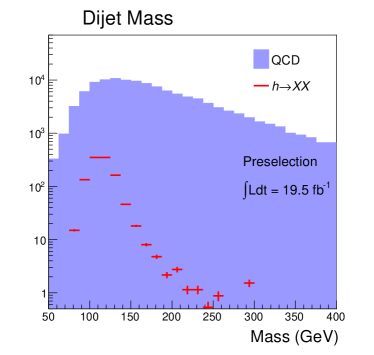
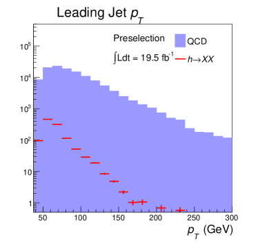
Figure 4: Distributions of some kinematic quantities after preselection. Left: $m_{jj}$, the invariant mass of the two leading jets in the event. Right: $p_{T}$ of the leading jet in the event. Shown here are simulated signal events and $b\bar{b}$ background, for a signal model with $m_{H}=125$ GeV/$c^{2}$ and $m_{X}=20$ GeV/$c^{2}$.

	Background		Signal
Cut	Number of events	Efficiency (%)	Number of events	Efficiency (%)
Trigger	7.4 x $10^{7}$	—	1.6 x $10^{4}$	—
Jet quality	1.2 x $10^{7}$	15.8	6.7 x $10^{3}$	42.4
Muon match	9.1 x $10^{6}$	78.2	4.7 x $10^{3}$	70.5
$\textrm{IPS}_{4}$	2.8 x $10^{5}$	3.1	1.4 x $10^{3}$	28.7
Mass window	6.8 x $10^{4}$	23.8	1.1 x $10^{3}$	80.7

Table 1: Efficiency of the various cuts applied in preselection (and the mass window cut). Each row shows the number of events passing the given cut, as well as all of those preceding it, and the relative efficiency of that cut for events which have passed all preceding cuts. All numbers are scaled to the 2012 CMS luminosity of 19.5 fb^-1.

In the final selection step, we look for properties of the jets which can be used to separate signal from the $b\bar{b}$ background. In general, the jets originating from our signal model have two key differences from the QCD background: first, they are expected to have more displaced tracks, and for these tracks to be more highly displaced (as the lifetimes of both the $X$ and the $b$ contribute to their displacement); and second, we expect the jets to exhibit substructure arising from the presence of the $b\bar{b}$ pair. After pre-selection, we thus apply stringent requirements on the displaced tracks and jet substructure for both jets using the variables described in Sections 3 and 4. The particular values used are as follows:

1. Dijet mass between (80,140) GeV/$c^{2}$

2. $\textrm{IPS}_{4}>25$ for both jets

3. $\tau_{21}<0.65$ for both jets

After the final selection, the QCD background is essentially eliminated. Figure 5 shows the mass distribution in the final signal region (except the mass window cut). However, since our cuts are selecting out sharply falling tails of the QCD background, Monte Carlo simulations can become very unreliable. At the LHC, data driven methods must be employed to obtain a reliable background estimate. We propose such a data-driven estimate in the next section.

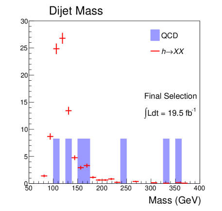
Figure 5: Distribution of $m_{jj}$, the invariant mass of the two leading jets in the event after final selection. All but the mass window cuts are applied. Shown here are simulated signal events and $b\bar{b}$ background, for a signal model with $m_{H}=125$ GeV/$c^{2}$ and $m_{X}=20$ GeV/$c^{2}$. The signal is clearly visible as a prominent peak over the background.

6 Background Estimation

We adopt a data-driven approach to estimate the expected background, in order to minimize the dependence on quantities which may not be well-modeled in the Monte Carlo simulation. We use a standard “ABCD” approach in order to estimate the expected amount of background in the signal region. Specifically, we take advantage of the fact that the two fat jets in an event, as they shower and decay independently, should have uncorrelated values for the displaced track and substructure variables.

We thus define our “signal” region for each individual jet as $\textrm{IPS}_{4}>25$ and $\tau_{21}<0.65$, and define our regions (given events that pass our preselection, including the mass window) as follows:

• Region A: both jets fail

• Region B: leading jet passes, second jet fails

• Region C: leading jet fails, second jet passes

• Region D: both jets pass (signal region)

The final background estimate is then obtained from the ratio $BC/A$. Table 2 shows the results of applying this technique to the background and signal simulation. We observe that the final estimate is consistent with the actual number of events in region D in simulation.

Region	Background	Signal
A (fail/fail)	6040 $\pm$ 220	22
B (pass/fail)	305 $\pm$ 50	47
C (fail/pass)	345 $\pm$ 53	38
D (pass/pass)	16 $\pm$ 12	77
Final estimate (BC/A)	17.4 $\pm$ 4.0

Table 2: The number of events in each region for our ABCD technique, scaled to the 2012 CMS luminosity of 19.5 fb^-1. The errors include both the statistical uncertainty (from our limited MC sample size) and the systematic uncertainty derived from comparison to the data sidebands; the latter is the dominant effect.

We can also crosscheck this method in two other ways: first, we can apply the same method but with a different mass window, in order to obtain a sideband selection of events. Using the background simulation, we get consistent results using a mass window of (100,160) or (120,180), although the expected signal in these regions is of course much less.

Another alternative crosscheck is to take advantage of the fact that the $\textrm{IPS}_{4}$ and $\tau_{21}$ variables are relatively uncorrelated, and thus can be used to define another pair of variables for applying the ABCD method. In this case, the statistics in the “B” region are relatively low, thus resulting in a larger systematic uncertainty, so we do not adopt this as our central estimate. However, we obtain an estimate of $20\pm 9$ events (statistical uncertainty only), consistent with our previous estimate.

7 Results

Applying the efficiency and the expected QCD background numbers shown in Tables 1 and 2, and using the luminosity collected at CMS in 2012 (19.5 fb^-1), we can set limits on the cross-section times branching ratio of the Higgs boson to $X\rightarrow b\bar{b}$. The limits are shown in Figure 6 and are obtained using CL_s test statistics and assuming a 50% total systematic uncertainty. The systematic uncertainty is conservatively estimated by examining the maximum deviation of the data-driven method when compared to the actual number of QCD events in different mass windows (which is limited by our QCD statistics in the higher mass windows). As seen from the figure, for the SM NLO cross-section and a branching ratio of 20%, we can exclude down to $c\tau>$ 3 mm for $m_{X}=$ 20 GeV/$c^{2}$. The limits for higher $m_{X}$ are worse due to softer jets and muons. For lower $m_{X}$, the tracks become more collimated and the $\tau_{21}$ variable becomes less effective. However, a 20% $h\rightarrow XX\rightarrow b\bar{b}b\bar{b}$ branching ratio can be consistently excluded for $m_{X}\in(15,25)$ GeV/$c^{2}$ at $c\tau>$ 3 mm. Further optimization for different mass points may be possible and we leave a detailed study to the experimental collaborations to properly take detector effects into account.

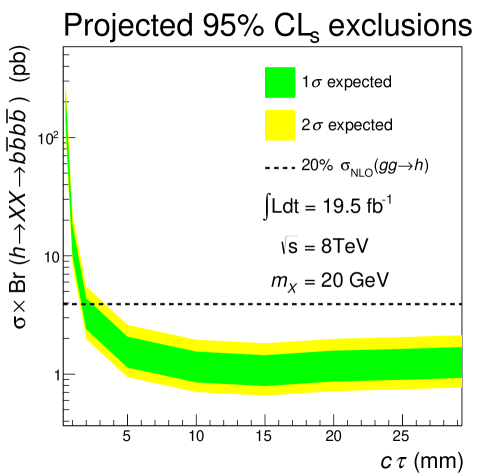
Figure 6: Expected limits on the cross-section times branching ratio of the process $h\rightarrow XX\rightarrow 4b$ given 19.5 fb^-1 of data, with 50% total uncertainty on the background. Systematic uncertainties on the luminosity and efficiency are not considered.

In Figure 7 we also consider the discovery potential for $h\rightarrow XX\rightarrow 4b$ decay. For a branching ratio of 20%, this new decay mode may be discoverable with the current 19.5 fb^-1 of 8 TeV LHC data for $m_{X}=$ 15 to 25 GeV/$c^{2}$.

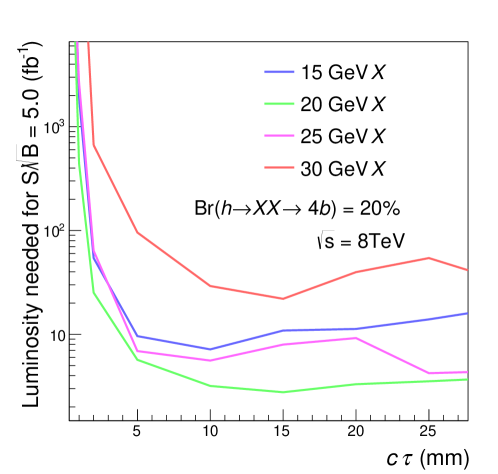
Figure 7: Luminosity needed to obtain 5$\sigma$ significance assuming a $20\%$ branching ratio of $h\rightarrow XX\rightarrow 4b$. Uncertainities are not included in this plot

8 Conclusion

In this note we have introduced several powerful kinematic cuts designed to discover a Higgs boson decaying to long-lived neutral particles. The unique features of this channel $h\rightarrow XX\rightarrow 4b$ are two-fold. First, the highly-displaced vertices resulting from the decay of the long-lived particles, some fraction of which occurs before reaching within the beampipe. The tracks from these vertices will have large IPS. Second, the long lived particles are boosted enough such the $b\bar{b}$ pairs are contained within one “fat jet”, removing combinatoric ambiguities and allowing us to take advantage of the jet substructure to distinguish the signal from the QCD background. We have developed a data-driven method to estimate the background and for certain values of the (pseudo-)scalar decay length and masses calculated the expected exclusion (Figure 6) and luminosity needed for discovery (Figure 7), showing that we have a strong discovery potential in this channel with about 19.5 fb^-1 of recorded LHC data.

Currently, the primarily limiting factor in this analysis is the trigger selection, as the existing triggers have a relatively low efficiency for the signal considered here. Given the importance of potential new discovery through exotic topologies that include long-lived particles decaying in the silicon tracker, the authors were led to evaluate a Graphics Processing Unit (GPU) enhancement of the existing High-Level Trigger (HLT) [39] to provide new complex triggers that were not previously feasible. The proposed new algorithms will allow for the first time the reconstruction of long-lived particles in the tracker system for the purpose of online selection. New ways of enhancing the trigger performance and the development of dedicated custom exotic triggers are the key for extending the reach of physics at the LHC.

As a final note, we re-iterate that this study is optimized on a specific mass point, $m_{X}=20$ GeV/$c^{2}$. A detailed optimization on the cuts on $\textrm{IPS}_{4}$ and $\tau_{21}$ could significantly improve the exclusion limits for different $X$ masses. Furthermore, even though we only focused on the $X\rightarrow b\bar{b}$ case, our techniques may be sensitive to other channels, such as $X\rightarrow\tau^{+}\tau^{-}$ or a Higgs boson decaying to a long-lived RPV neutralino $\chi$, which then decays into $\nu b\bar{b}$. With improved triggers for long-lived particles, additional searches for long-lived $X\rightarrow gg$ and $X\rightarrow qqq$ (for fermionic $X$) may also be possible. Our search channel also does not have to be limited to a 125 GeV/$c^{2}$ Higgs particle. New particles may potentially be discovered through these long-lived decays. We leave a detailed optimization of the different cuts for different decay channels for future work.

Appendix A Validations

In this section, we describe how we obtain a K-factor of 1.6 and validate our IPS variables against published results. A separate 7 TeV $b\bar{b}$ sample is generated for this purpose (matched up to four jets). 500 thousand events were generated using MadGraph 5 v1.5.7 with the same settings as those listed in Section 2. The final state particles are clustered using anti-$k_{T}$ algorithm and their momentum smeared with resolution parameters from CMS  [33]. We reproduce the CMS analysis in [29] using the quoted $b$-quark tagging efficiencies and mistag rates. A K-factor of 1.6 is obtained by matching our dijet mass distribution against Figure 4a in [29]. The resulting distribution is shown in Figure 8.

To study the effects of fake $b$-tags in events without a true $b$-quark, another 9 million 8 TeV $c\bar{c}$ events were generated using MadGraph 5 v1.5.7 (matched up to 4 jets), and no events passing preselection cuts are found. This suggests that the rate of fake $b$-tags in our analysis described can be safely neglected. It should be noted that the K-factor obtained from Figure 8 also includes the effects of mistags arising from light-quark contamination; since our pre-selection cuts are much more stringent than the analysis in [29], using this K-factor should conservatively include any effects that we might see from fake $b$-tags, so our ignoring of the light flavor QCD background is justified. The analysis in [29] also indicates that vector boson processes contribute less than 1% of the total background, hence we neglect their contributions to the background as well.

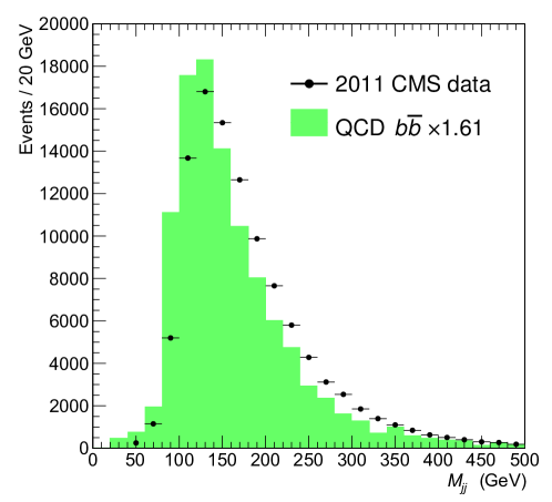
Figure 8: The mass distribution of the two leading jets as compared to the CMS analysis in [29]. A K-factor of 1.6 is obtained and serves as a conservative estimate of $c\bar{c}$ and light flavor contaminations.

To validate our displaced jet variables outlined in Section 3, we also use our 7 TeV validation sample and compare the IPS distributions to the published results in Figure 3 in [34]. The normalized distributions are shown in Figure 9. Modest disagreements are seen at large IPS. However, the deviations are smaller than our 50% systematic uncertainty. Given the systematic deviations, we also refrain from pushing our $\textrm{IPS}_{4}$ cut beyond 25, and our exclusion results are conservative.

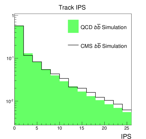
Figure 9: The normalized IPS distribution for $b$-jets when compared to published CMS results in [34].

References

- [1] G. Aad et al. [ATLAS Collaboration], Observation of a new particle in the search for the Standard Model Higgs boson with the ATLAS detector at the LHC, Phys. Lett. B 716 (2012) 1 [arXiv:1207.7214 [hep-ex]].
- [2] S. Chatrchyan et al. [CMS Collaboration], Observation of a new boson at a mass of 125 GeV with the CMS experiment at the LHC, Phys. Lett. B 716 (2012) 30 [arXiv:1207.7235 [hep-ex]].
- [3] [ATLAS Collaboration], Combined coupling measurements of the Higgs-like boson with the ATLAS detector using up to 25 fb-1 of proton-proton collision data, ATLAS-CONF-2013-034.
- [4] [CMS Collaboration], Combination of standard model Higgs boson searches and measurements of the properties of the new boson with a mass near 125 GeV, CMS-PAS-HIG-13-005.
- [5] G. Belanger, B. Dumont, U. Ellwanger, J. F. Gunion and S. Kraml, Status of invisible Higgs decays, arXiv:1302.5694 [hep-ph].
- [6] J. Ellis and T. You, Updated Global Analysis of Higgs Couplings, arXiv:1303.3879 [hep-ph].
- [7] M. J. Strassler and K. M. Zurek, Discovering the Higgs through highly-displaced vertices, Phys. Lett. B 661, 263 (2008) [hep-ph/0605193].
- [8] S. Chang, P. J. Fox and N. Weiner, Naturalness and Higgs decays in the MSSM with a singlet, JHEP 0608, 068 (2006) [hep-ph/0511250].
- [9] L. M. Carpenter, D. E. Kaplan and E. -J. Rhee, Reduced fine-tuning in supersymmetry with R-parity violation, Phys. Rev. Lett. 99, 211801 (2007) [hep-ph/0607204].
- [10] V. M. Abazov et al. [D0 Collaboration], Search for Resonant Pair Production of long-lived particles decaying to b anti-b in p anti-p collisions at s**(1/2) = 1.96-TeV, Phys. Rev. Lett. 103 (2009) 071801 [arXiv:0906.1787 [hep-ex]].
- [11] G. Aad et al. [ATLAS Collaboration], Search for long-lived, heavy particles in final states with a muon and multi-track displaced vertex in proton-proton collisions at TeV with the ATLAS detector, Phys. Lett. B 719 (2013) 280 [arXiv:1210.7451 [hep-ex]].
- [12] R. Dermisek and J. F. Gunion, Escaping the large fine tuning and little hierarchy problems in the next to minimal supersymmetric model and h —¿ aa decays, Phys. Rev. Lett. 95, 041801 (2005) [hep-ph/0502105].
- [13] R. Barbier, C. Berat, M. Besancon, M. Chemtob, A. Deandrea, E. Dudas, P. Fayet and S. Lavignac et al., R-parity violating supersymmetry, Phys. Rept. 420, 1 (2005) [hep-ph/0406039].
- [14] D. Aristizabal Sierra, W. Porod, D. Restrepo and C. E. Yaguna, Novel Higgs decay signals in R-parity violating models, Phys. Rev. D 78, 015015 (2008) [arXiv:0804.1907 [hep-ph]].
- [15] J. Kang and M. A. Luty, Macroscopic Strings and ’Quirks’ at Colliders, JHEP 0911, 065 (2009) [arXiv:0805.4642 [hep-ph]].
- [16] K. Cheung, W. -Y. Keung and T. -C. Yuan, Phenomenology of iquarkonium, Nucl. Phys. B 811, 274 (2009) [arXiv:0810.1524 [hep-ph]].
- [17] B. Bellazzini, C. Csaki, A. Falkowski and A. Weiler, Buried Higgs, Phys. Rev. D 80, 075008 (2009) [arXiv:0906.3026 [hep-ph]].
- [18] J. E. Juknevich, D. Melnikov and M. J. Strassler, A Pure-Glue Hidden Valley I. States and Decays, JHEP 0907 (2009) 055 [arXiv:0903.0883 [hep-ph]].
- [19] A. Falkowski, J. T. Ruderman, T. Volansky and J. Zupan, Hidden Higgs Decaying to Lepton Jets, JHEP 1005, 077 (2010) [arXiv:1002.2952 [hep-ph]].
- [20] C. Englert, J. Jaeckel, E. Re and M. Spannowsky, Evasive Higgs Maneuvers at the LHC, Phys. Rev. D 85, 035008 (2012) [arXiv:1111.1719 [hep-ph]].
- [21] P. W. Graham, D. E. Kaplan, S. Rajendran and P. Saraswat, Displaced Supersymmetry, JHEP 1207, 149 (2012) [arXiv:1204.6038 [hep-ph]].
- [22] M. J. Strassler and K. M. Zurek, Echoes of a hidden valley at hadron colliders, Phys. Lett. B 651, 374 (2007) [arXiv:hep-ph/0604261].
- [23] M. Cacciari, G. P. Salam and G. Soyez, The Anti-k(t) jet clustering algorithm, JHEP 0804, 063 (2008) [arXiv:0802.1189 [hep-ph]].
- [24] K. T. Matchev and S. D. Thomas, Higgs and boson signatures of supersymmetry, Phys. Rev. D 62, 077702 (2000) [arXiv:hep-ph/9908482].
- [25] T. Sjostrand, S. Mrenna and P. Z. Skands, PYTHIA 6.4 Physics and Manual, JHEP 0605, 026 (2006) [hep-ph/0603175].
- [26] LHC Higgs Cross Section Working Group, S. Heinemeyer, C. Mariotti, G. Passarino, and R. Tanaka (Eds.), Handbook of LHC Higgs Cross Sections: 3. Higgs Properties, arXiv:1201.3084 [hep-ph].
- [27] J. Alwall, M. Herquet, F. Maltoni, O. Mattelaer and T. Stelzer, MadGraph 5 : Going Beyond, JHEP 1106, 128 (2011) [arXiv:1106.0522 [hep-ph]].
- [28] M. L. Mangano, M. Moretti, F. Piccinini and M. Treccani, Matching matrix elements and shower evolution for top-quark production in hadronic collisions, JHEP 0701, 013 (2007) [hep-ph/0611129].
- [29] S. Chatrchyan et al. [CMS Collaboration], Search for a Higgs boson decaying into a b-quark pair and produced in association with b quarks in proton-proton collisions at 7 TeV, Phys. Lett. B 722, 207 (2013) [arXiv:1302.2892 [hep-ex]].
- [30] J. Pumplin, D. R. Stump, J. Huston, H. L. Lai, P. M. Nadolsky and W. K. Tung, New generation of parton distributions with uncertainties from global QCD analysis, JHEP 0207, 012 (2002) [hep-ph/0201195].
- [31] [CMS Collaboration], Tracking and Primary Vertex Results in First 7 TeV Collisions, CMS-PAS-TRK-10-005.
- [32] M. Cacciari, G. P. Salam and G. Soyez, FastJet User Manual, Eur. Phys. J. C 72, 1896 (2012) [arXiv:1111.6097 [hep-ph]].
- [33] [CMS Collaboration], Particle-Flow Event Reconstruction in CMS and Performance for Jets, Taus, and MET, CMS-PAS-PFT-09-001.
- [34] A. Rizzi, F. Palla and G. Segneri, Track impact parameter based b-tagging with CMS, CERN-CMS-NOTE-2006-019.
- [35] S. Chatrchyan et al. [CMS Collaboration], Identification of b-quark jets with the CMS experiment, JINST 8, P04013 (2013) [arXiv:1211.4462 [hep-ex]].
- [36] J. Thaler and K. Van Tilburg, Identifying Boosted Objects with N-subjettiness, JHEP 1103, 015 (2011) [arXiv:1011.2268 [hep-ph]].
- [37] J. Thaler and K. Van Tilburg, Maximizing Boosted Top Identification by Minimizing N-subjettiness, JHEP 1202, 093 (2012) [arXiv:1108.2701 [hep-ph]].
- [38] D. Krohn, J. Thaler and L. -T. Wang, Jet Trimming, JHEP 1002, 084 (2010) [arXiv:0912.1342 [hep-ph]].
- [39] V. Halyo, A. Hunt, P. Jindal, P. LeGresley and P. Lujan, GPU Enhancement of the Trigger to Extend Physics Reach at the LHC, JINST 1310, P10005 (2013) [arXiv:1305.4855 [physics.ins-det]].