Curvature-induced Rashba spin-orbit interaction in strain-driven nanostructures

Abstract

We derive the effective dimensionally reduced Schrödinger equation with spin-orbit interaction in low-dimensional electronic strain driven nanostructures. A method of adiabatic separation among fast normal quantum degrees of freedom and slow tangential quantum degrees of freedom is used to show the emergence of a strain-induced Rashba-like spin-orbit interaction (SOI). By applying this analysis to one-dimensional curved quantum wires we demonstrate that the curvature-induced Rashba SOI leads to enhanced spin-orbit effects.

I Introduction

The interest in the theory of quantum physics on bent manifolds has received a boost since the experimental progresses in synthesizing low-dimensional nanostructures with curved geometries – the next generation nanodevices ahn06 ; ko10 ; mei07 ; par10 . From a purely theoretical point of view, the problem of the quantum motion of a particle living in a curved space has represented a matter of controversy for a long time dew57 ; jen71 ; dac82 ; kap97 . The problem arises because Dirac quantization on a curved manifold leads to operator-ordering ambiguitiesdew57 . However, Jensen and Koppe jen71 and later da Costa dac82 (JKC) have introduced a thin-wall quantisation procedure that circumvents this pitfall. It treats the quantum motion on a curved two-dimensional (2D) surface – or analogously on a torsionless planar one-dimensional (1D) curved manifold – as the limiting case of a particle in three-dimensional (3D) space subject to lateral quantum confinement. For both 1D curved manifold and 2D surface with a translational invariant direction, the JKC method allows to eliminate the surface curvature from the effective dimensionally reduced Schrödinger equation at the expense of adding a potential term to it. The problem is therefore substantially simplified, since quantum carriers can actually live in a 2D or 1D space in the presence of a curvature-induced quantum geometric potential (QGP). On the nanoscale, the QGP can actually cause many intriguing phenomena can00 ; aok01 ; enc03 ; fuj05 ; kos05 ; gra05 ; cha04 ; mar05 . For instance, a quantum particle constrained to a periodically curved surface senses a periodic QGP acting as a topological crystalaok01 . Likewise the QGP in spirally rolled-up nanostructures leads to winding-generated bound statesved00 ; ort10 . The experimental observation of these fascinating phenomena is hindered by the fact that in actual systems with curvature radii on the order of a few hundred nanometers, the QGP is still very weak – it is in magnitude proportional to $\hbar$ – and typically only comes into play on the sub-Kelvin energy scale. It has been recently shown ort11b that by accounting for the effect of the deformation potentials of the model-solid theory van89 ; sun10 , the strain field induced by the curvature leads to a strain-induced geometric potential (SGP) which has the same functional form as the QGP but strongly boosting it. One cannot therefore distinguish between curvature-induced quantum effects and curvature-induced classical strain effects in nanosystems – they are always present and contribute in different amount to the same geometric potential.

In this work, we show that this strain field of bent nanostructures leads to a curvature-induced Rashba spin-orbit interaction whose strength follows precisely the local curvature of the manifold. This is immediately relevant for electronic nanodevices since the modern nanostructuring methodahn06 ; ko10 is based on the tendency of thin films detached from their substrates to assume a shape yielding the lowest possible elastic energy. As a result, thin films can either roll up into tubessch01 ; pri00 or undergo wrinkling to form nanocorrugated structuresfed06 ; mei07 ; cen09 . The nanoscale variation of the strain represents a key property of such bent nanostructures. It leads to considerable band-edge shiftsden10 with regions under tensile and compressive strain shifting in opposite directions. Strain is thus widely used and applied in nanosystems and here we put forward that it intrinsically leads to spin-orbit effects. We apply this theoretical framework to both curved two-dimensional systems and one-dimensional curved quantum wires, showing that in the latter case two different Rashba-like spin-orbit interactions come into play enhancing spin-orbit splittings.

II Curved two-dimensional systems

In the thin-wall quantization procedure, quantum excitation energies in the normal direction are raised far beyond those in the tangential direction. This allows to neglect the quantum motion in the normal direction and derive an effective, dimensionally reduced, Schrödinger equation. As opposed to a classical particle, a quantum particle constrained to a curved surface retains some knowledge of the surrounding 3D space. In spite of the absence of interactions, it indeed experiences the well-known attractive QGP dac82 . It has been shown that the JKC thin-wall quantization procedure to derive the effective Schrödinger equation is well-founded, also in the presence of externally applied electric and magnetic fieldsfer08 ; ort11 . Empirical evidence for the validity of this approach is provided by the experimental realization of an optical analogue of the curvature-induced geometric potentialsza10 .

In order to derive the effective Hamiltonian for a curved two-dimensional electron gas with spin-orbit interaction (SOI), we therefore use the same conceptual framework of the JKC thin-wall quantization procedure jen71 . The mathematical description is set by defining a 3D curvilinear coordinate system for the tubular nanostructure. We parameterize the stress-free surface ${\cal S}$ as ${\bf r}={\bf r}(s,z)$ where $z$ indicates the coordinate along the translationally invariant direction of the the tubular nanostructure and $s$ corresponds to the arclength along the curved direction of the thin film. The entire portion of the nanostructure can be similarly parameterized as ${\bf R}(s,z,q_{3})={\bf r}(s,z)+q_{3}\hat{N}(s)$ where $\hat{N}(s)$ indicates the unit vector normal to the bent direction of the thin film and is oriented so that regions with $q_{3}>0$ are under compressive strain for positive values of the radius of curvature and under tensile strain for negative ones [see Fig.1]. The strain distribution of the thin film can be easily derived assuming the in-plane strain conditioncho92 ${\epsilon}_{zz}\equiv 0$. This can be justified in nanostructures with a characteristic dimension along the $z$ direction much larger than the structural dimensions in the remaining coordinates. Following Landau lan86 , the strain component along the bent structure of the thin film reads $\epsilon_{s\,s}=-q_{3}\kappa(s)$ where $\kappa(s)$ indicates the only non-vanishing principal curvature of the curved stress-free two-dimensional manifold. The remaining strain component in the normal direction $q_{3}$ is related to $\epsilon_{ss}$ by $\epsilon_{q_{3}q_{3}}=-\left[\nu/(1-\nu)\right]\epsilon_{ss}$ with $\nu$ the Poisson ratio.

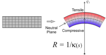
Figure 1: Cross section of a portion of the bent nanostructure with negative value of the radius of curvature. The effect of curvature leads to regions under tensile strain for $q_{3}>0$ and compressive one for $q_{3}<0$

As the linear deformation potential theory van89 predicts a strain-induced shift of the conduction band, local variations of the strain thus render a local potential for the conducting electrons ${\cal V}_{\epsilon}(s,q_{3})=\gamma\kappa(s)q_{3}$ which always implies an attraction towards the tensile regions of the thin film. Here we have introduced the characteristic energy scale $\gamma$, proportional to the hydrostatic deformation potential of the conduction valley of the nanostructure, which typically lies in the eV scale for conventional semiconductors van89 . As the strain field produces an asymmetric confining potential along the normal direction of the bent surface, it will immediately yield an average electric field $E\,\hat{N}(s)$ whose strength is proportional to the curvature of the nanostructure. The strain field therefore leads to a curvature-induced Rashba SOI. The resulting Schrödinger equation in the effective mass approximation will thus read

$$-\dfrac{\hbar^{2}}{2m^{\star}}G^{ij}{\cal D}_{i}{\cal D}_{j}\psi+{\cal V}_{\epsilon}(s,q_{3})\psi+\dfrac{\alpha}{\hbar}\,{\bm{\sigma}}\cdot{\bf p}\,\times{\hat{N}(s)}\psi=E\psi.$$ (1)

where we adopted Einstein summation convention, ${\bm{\sigma}}$ is the Pauli matrix vector and ${\bf p}$ the ordinary momentum operator in Cartesian coordinates. In Eq.1, $G^{ij}$ corresponds to the 3D metric tensor which for our coordinate system takes the simple diagonal form

$$G_{ij}=\left(\begin{array}[]{ccc}H(s)^{2}&0&0\\ 0&1&0\\ 0&0&1\end{array}\right),$$ (2)

with $H(s)=1-\kappa(s)q_{3}$. Finally the covariant derivative ${\cal D}_{i}$ is defined as ${\cal D}_{i}=\partial_{i}v_{j}-\Gamma_{i\,j}^{k}v_{k}$ with $v_{j}$ the covariant components of a generic 3D vector field, and $\Gamma_{i\,j}^{k}$ representing the Christoffel symbols

$$\Gamma_{ij}^{k}=\dfrac{1}{2}G^{kl}\left[G_{il,i}+G_{il,j}-G_{ii,j}\right].$$

With this, the Schrödinger equation Eq. 1 can be simply expanded in our curvilinear coordinate system as

$$E\,\psi = \left[-\dfrac{\hbar^{2}}{2m^{\star}\,H(s)}\partial_{s}\left(\dfrac{1}{H(s)}\partial_{s}\right)-\dfrac{\hbar^{2}}{2m^{\star}\,H(s)}\partial_{q_{3}}\right.$$ (3)

$$\left.\left(H(s)\,\partial_{q_{3}}\right)-\dfrac{\hbar^{2}}{2m^{\star}}\partial^{2}_{y}+{\cal V}_{\epsilon}(s,q_{3})+{\cal V}_{\lambda}(q_{3})\right]\psi$$

$$-i\alpha\left(\sigma_{s}\partial_{y}-\dfrac{\sigma_{y}}{H(s)}\partial_{s}\right)\psi,$$

where $\sigma_{s}={\bm{\sigma}}\cdot{\hat{s}}$ and the momentum along the bent direction of the nanostructure is $p_{s}\equiv-i\hbar G^{s\,s}\partial_{s}$ . We have also introduced a squeezing potential in the normal direction ${\cal V}_{\lambda}(q_{3})$. In Ref. ort11b this was assumed to be given by two infinite step potential barriers at $\pm\delta/2$ with $\delta$ the total thickness of the thin film. In the remainder we will instead consider the case of an harmonic trap ${\cal V}_{\lambda}(q_{3})=\lambda q_{3}^{2}/2$ to show that the ensuing results are not dependent on the specific form of the squeezing potential at hand. To proceed further we introduce, in the same spirit of the thin-wall quantization procedure, a rescaled wavefunction $\chi=\psi\times\sqrt{H(s)}$ for which the surface density probability is defined as $\int|\chi(s,y,q_{3})|^{2}dq_{3}$. The resulting Schrödinger equation is then determined by an effective Hamiltonian

$${\cal H} = -\dfrac{\hbar^{2}}{2m^{\star}}\partial_{z}^{2}-\dfrac{\hbar^{2}}{2m^{\star}}\dfrac{\partial_{s}^{2}}{H(s)^{2}}+\dfrac{\hbar^{2}}{m^{\star}}\dfrac{\partial_{s}H(s)\,\partial_{s}}{H(s)^{3}}$$ (4)

$$-\dfrac{\hbar^{2}}{2m^{\star}}\partial_{q_{3}}^{2}-\dfrac{\hbar^{2}}{2m^{\star}}\,\left[\dfrac{5}{4}\,\dfrac{\left(\partial_{s}H(s)\right)^{2}}{H(s)^{4}}-\dfrac{\partial_{s}^{2}H(s)}{2\,H(s)^{3}}\right]$$

$$-\dfrac{\hbar^{2}}{2m^{\star}}\dfrac{\left(\partial_{q_{3}}H(s)\right)^{2}}{4\,H(s)^{2}}+{\cal V}_{\lambda}(q_{3})+{\cal V}_{\epsilon}(s,q_{3})$$

$$-i\alpha\left(\sigma_{s}\partial_{z}-\sigma_{z}\dfrac{\partial_{s}}{H(s)}\right)+i\alpha\sigma_{z}\dfrac{\partial_{s}H(s)}{H(s)^{\frac{3}{2}}}.$$

For large enough strength of the squeezing potential in the normal direction, we can follow Ref. ort11b and expand the Hamiltonian of Eq.4 as ${\cal H}=\sum_{k}q_{3}^{k}{\cal H}_{k}$. At the zeroth order in $q_{3}$ and retaining the leading order correction linear in $q_{3}$, the effective Hamiltonian reads:

$${\cal H}_{0} = -\dfrac{\hbar^{2}}{2m^{\star}}\partial_{z}^{2}-\dfrac{\hbar^{2}}{2m^{\star}}\partial_{s}^{2}-\dfrac{\hbar^{2}}{2m^{\star}}\partial_{q_{3}}^{2}-\dfrac{\hbar^{2}\kappa(s)^{2}}{8m^{\star}}$$ (5)

$$-i\alpha\left(\sigma_{s}\partial_{z}-\sigma_{z}\partial_{s}\right)+{\cal V}_{\lambda}(q_{3})+{\cal V}_{\epsilon}(s,q_{3}).$$

The strong size quantisation along the normal direction allows to employ the adiabatic approximation and consider an ansatz for the wave function $\chi(s,z,q_{3})=\chi^{T}(s,q_{z})\times\chi^{N}(s,q_{3})$ with $\chi_{N}(s,q_{3})$ solving at fixed $s$ the one-dimensional Schrödinger equation for the fast normal degrees of freedom which is regulated by the Hamiltonian

$${\cal H}_{0}^{N}=-\dfrac{\hbar^{2}}{2m^{\star}}\partial_{q_{3}}^{2}+\gamma\kappa(s)q_{3}+\dfrac{1}{2}\lambda q_{3}^{2}.$$ (6)

The spectrum of the Hamiltonian above can be easily read as $E^{N}=\hbar\sqrt{\lambda/m}\left(n+1/2\right)-\gamma^{2}\kappa(s)^{2}/\lambda$. With this, the effective Hamiltonian for the slow tangential quantum degrees of freedom can be found by integrating out the $q_{3}$ degrees of freedom. We then get the dimensionally reduced effective Hamiltonian

$${\cal H}_{0}^{T}=-\dfrac{\hbar^{2}}{2m^{\star}}\partial_{z}^{2}-\dfrac{\hbar^{2}}{2m^{\star}}\partial_{s}^{2}-\dfrac{S^{2}\kappa(s)^{2}}{8m^{\star}}-i\alpha\left(\sigma_{s}\partial_{z}-\sigma_{z}\partial_{s}\right).$$ (7)

It has the same functional form of the effective Hamiltonian for a planar two-dimensional electron gas with Rashba spin-orbit interaction and a geometric potential whose magnitude $S^{2}=\hbar^{2}+8m^{\star}\gamma^{2}/\lambda$ is strongly renormalised by the strain-induced geometric potential ort11b . We point out that for systems with an intrinsic SOI the normal and tangential degrees of freedom, curvature induced geometric potential proportional to the mean curvature of the manifold can appear  chang2013 . These terms are absent in the strain-induced Rashba spin-orbit coupling because of the presence of the normal potential gradient.

We next use this theoretical framework to derive the effective dimensionally reduced Hamiltonian considering the case of a rolled-up cylindrical nanotube and a nanocorrugated thin film. For a cylindrical nanotube of radius $R$ the arclength can be easily expressed in cylindrical coordinates as $s=R\phi$ and the resulting effective Hamiltonian for a cylindrical two-dimensional electron gas (C2DEG) then reads tru07

$${\cal H}_{C2DEG} = -\dfrac{\hbar^{2}}{2m^{\star}}\partial_{z}^{2}-\dfrac{\hbar^{2}}{2m^{\star}R^{2}}\partial_{\phi}^{2}$$ (8)

$$-i\alpha\left(\sigma_{\phi}\partial_{z}-\sigma_{z}\dfrac{\partial_{\phi}}{R}\right),$$

where we have neglected the geometric potential since it corresponds to a rigid shift of the energies. For a nanocorrugated thin film instead, we start out by parametrizing the stress-free surface in the Monge gauge as $y=h(x)$ with $h$ indicating the height of the corrugation with respect to its planar counterpart. In Cartesian coordinates then the effective Hamiltonian reads

$${\cal H}_{NC} = -\dfrac{\hbar^{2}}{2m^{\star}}\partial_{z}^{2}-\dfrac{\hbar^{2}}{2m^{\star}}\dfrac{1}{1+h^{\prime}(x)^{2}}\partial_{x}^{2}$$

$$-\dfrac{S^{2}}{8m^{\star}}\dfrac{h^{\prime\prime}(x)^{2}}{\left[1+h^{\prime}(x)\right]^{3}}$$

$$-\dfrac{i\alpha}{\sqrt{1+h^{\prime}(x)^{2}}}\left(\sigma_{x}\partial_{z}+\sigma_{y}h^{\prime}(x)\partial_{z}-\sigma_{z}\partial_{x}\right)$$

III Curved quantum wires

We now apply the theoretical framework we developed in the previous section to planar curved one-dimensional electron gases. In this case, due to the asymmetric confinement in the direction perpendicular to the plane of the curved one-dimensional systems ($\hat{z}$ following the definition of the curvilinear coordinate system given in Sec.II) there is an additional Rashba SOI different from the strain-induced one. The effective Schrödinger equation reads

$$E\psi = -\dfrac{\hbar^{2}}{2m^{\star}}G^{ij}{\cal D}_{i}{\cal D}_{j}\psi+{\cal V}_{\epsilon}(s,q_{3})\psi+$$ (10)

$$\dfrac{\alpha}{\hbar}\,{\bm{\sigma}}\cdot{\bf p}\,\times{\hat{N}(s)}\psi+(\dfrac{\alpha_{R}}{\hbar}\,{\bm{\sigma}}\cdot{\bf p}\,\times{\hat{z}})\psi$$

Since there is no coupling among the curvature of the one-dimensional planar wire and the direction normal to the plane, we can safely neglect the degrees of freedom in its direction. By expanding Eq.10 by covariant calculus we get the Schrödinger equation in the planar two-dimensional space as

$$E\,\psi = \left[-\dfrac{\hbar^{2}}{2m^{\star}\,H(s)}\partial_{s}\left(\dfrac{1}{H(s)}\partial_{s}\right)-\dfrac{\hbar^{2}}{2m^{\star}\,H(s)}\partial_{q_{3}}\right.$$

$$\left.\left(H(s)\,\partial_{q_{3}}\right)+{\cal V}_{\epsilon}(s,q_{3})+{\cal V}_{\lambda}(q_{3})\right]\psi$$

$$+i\alpha\left(\dfrac{\sigma_{z}}{H(s)}\partial_{s}\right)\psi-i\alpha_{R}\left(\dfrac{\sigma_{N}}{H(s)}\partial_{s}-\sigma_{s}\partial_{q_{3}}\right)\psi,$$

where $\sigma_{N}={\bm{\sigma}}\cdot\hat{N}(s)$.

The effective dimensionally reduced one-dimensional Schrödinger equation can be found by first performing a scaling of the wavefunction so that the one-dimensional surface density probability reads $\int|\chi(s,q_{3})|^{2}dq_{3}$, then expanding the resulting Hamiltonian as in Sec.II and finally employing the method of adiabatic separation among the fast normal quantum degree of freedom $q_{3}$ an the planar slow quantum degree of freedom $s$. The resulting effective Hamiltonian is

$${\cal H}_{0} = -\dfrac{\hbar^{2}}{2m^{\star}}\partial_{s}^{2}-\dfrac{S^{2}\kappa(s)^{2}}{8m^{\star}}+i\alpha\sigma_{z}\partial_{s}$$ (12)

$$-i\alpha_{R}\left(\sigma_{N}\partial_{s}-\dfrac{1}{2}\sigma_{s}\kappa(s)\right),$$

which agrees with the Hamiltonian for a curved one-dimensional quantum wire proposed in Ref. zha07 once the strain-induced Rashba SOI is neglected. To analyse the influence of the latter, we now consider the example of a closed quantum ring mei02 shown schematically in Fig.2 .

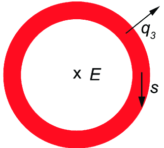
Figure 2: Schematics of the ring nanostructure. The electric field in the direction normal to the plane is due to an asymmetric confinement. Strain effects instead render an electric field in the direction $q_{3}$ normal to the ring.

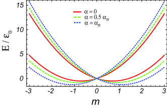
Figure 3: The bandstructure for a closed ring with strength of the Rashba SOI in the direction perpendicular to the plane $\alpha_{R}=\hbar^{2}/(2m^{\star}R)$ and different values of the strain-induced Rashba SOI $\alpha$. Energies are measured in units of $\epsilon_{0}=\hbar^{2}/(2m^{\star}R^{2})$. The spin-orbit splitting is generally enhanced by the effect of the Rashba SOI.

Adopting polar coordinates we have

$$\sigma_{s} = \sigma_{x}\sin{\phi}-\sigma_{y}\cos{\phi}$$

$$\sigma_{N} = \sigma_{x}\cos{\phi}+\sigma_{y}\sin{\phi},$$ (13)

whereas $s=R\phi$. With this, the effective Hamiltonian for the 1D ring can be then solved using a trial spinorial wave function of the form $\chi=\left[\chi_{1}\mathrm{e}^{i(m-1/2)\phi},\chi_{2}\mathrm{e}^{i(m+1/2)\phi}\right]^{T}$ where $m$ can only assume half-integer values to fulfill the periodic boundary conditions. The amplitude $\chi_{1}$ and $\chi_{2}$ depends on $m$. The corresponding energy spectrum can be simply found as

$$E(m) = \dfrac{\hbar^{2}}{2m^{\star}R^{2}}(m^{2}+\dfrac{1}{4})+\dfrac{\alpha}{2R}$$ (14)

$$\pm|m|\sqrt{\left(\dfrac{\hbar^{2}}{2m^{\star}R^{2}}+\dfrac{\alpha}{R}\right)^{2}+\dfrac{\alpha_{R}^{2}}{R^{2}}}.$$

As shown in Fig.3 the strain-induced Rashba SOI enhances the spin-orbit splitting due to the Rashba SOI in the direction perpendicular to the plane. The spin properties of the eigenstates of the Hamiltonian in Eq. 12 are not modified by the presence of the strain-induced Rashba SOI. Indeed, the expectation values for $\sigma_{s}$ and $\sigma_{N}$ are $\langle\chi|\sigma_{s}|\chi\rangle=0$ and $\langle\chi|\sigma_{N}|\chi\rangle=2\chi_{1}\,\chi_{2}$, respectively. This implies that the averaged spin projection, as expected, is pointing perpendicularly to the ring along the radial direction while the tangential component is vanishing. There is also a non trivial $z-$projection which is given by $\langle\chi|\sigma_{z}|\chi\rangle=\chi_{1}^{2}-\chi_{2}^{2}$ which is a characteristic signature of curvature effects. Hence, the presence of the strain-induced Rashba SOI affects only the intensity of the averaged spin projections by modifying the spinorial components of the wave function $\chi$. In particular, such term tends to enhance the out-of-plan spin projection. We expect this contribution to amplify the curvature effects on the spin transport properties of quantum rings liu .

IV Conclusions

We have derived, in conclusion, a dimensionally reduced Schrödinger equation with spin-orbit interaction in two-dimensional and effective one-dimensional electronic strain-driven nanostructures. By employing a method of adiabatic separation of fast and slow quantum degrees of freedom, we have shown that the effects of a finite curvature are twofold. First, in agreement with Ref. ort11b , the strain effects render an often gigantic renormalisation of the curved-induced quantum geometric potential. Second, the asymmetric confinement due to the strain field leads to a Rashba-type spin-orbit interaction whose strength is proportional to the local curvature of the nanostructure. Applying this theoretical framework to one-dimensional curved quantum wires leads to an enhanced spin-orbit splitting due to the presence of two Rashba-type SOI. The inclusion of strain effects therefore boosts the SOI which will strongly affect the electron spin transport properties of strain-driven nano structures in curved geometries.

References

- (1) J.-H. Ahn, H.-S. Kim, K. J. Lee, S. Jeon, S. J. Kang, Y. Sun, R. G. Nuzzo, and J. A. Rogers, Science 314, 1754 (2006).
- (2) H. Ko, K. Takei, R. Kapadia, S. Chuang, H. Fang, P. W. Leu, K. Ganapathi, E. Plis, H. S. Kim, S.-Y. Chen, M. Madsen, A. C. Ford, Y.-L. Chueh, S. Krishna, S. Salahuddin, and A. Javey, Nature 468, 286 (2010).
- (3) Y. Mei, S. Kiravittaya, M. Benyoucef, D. J. Thurmer, T. Zander, C. Deneke, F. Cavallo, A. Rastelli, and O. G. Schmidt, Nano Letters 7, 1676 (2007).
- (4) S.-I. Park, A.-P. Le, J. Wu, Y. Huang, X. Li, and J. A. Rogers, Advanced Materials 22, 3062 (2010).
- (5) B. S. DeWitt, Rev. Mod. Phys. 29, 377 (1957).
- (6) H. Jensen and H. Koppe, Annals of Physics 63, 586 (1971).
- (7) R. C. T. da Costa, Phys. Rev. A 23, 1982 (1981).
- (8) L. Kaplan, N. T. Maitra, and E. J. Heller, Phys. Rev. A 56, 2592 (1997).
- (9) G. Cantele, D. Ninno, and G. Iadonisi, Phys. Rev. B 61, 13730 (2000).
- (10) H. Aoki, M. Koshino, D. Takeda, H. Morise, and K. Kuroki, Phys. Rev. B 65, 035102 (2001).
- (11) M. Encinosa and L. Mott, Phys. Rev. A 68, 014102 (2003).
- (12) N. Fujita and O. Terasaki, Phys. Rev. B 72, 085459 (2005).
- (13) M. Koshino and H. Aoki, Phys. Rev. B 71, 073405 (2005).
- (14) J. Gravesen and M. Willatzen, Phys. Rev. A 72, 032108 (2005).
- (15) A. V. Chaplik and R. H. Blick, New J Phys. 6, 33 (2004).
- (16) A. Marchi, S. Reggiani, M. Rudan, and A. Bertoni, Phys. Rev. B 72, 035403 (2005).
- (17) A. I. Vedernikov and A. V. Chaplik, JETP 90, 397 (2000).
- (18) C. Ortix and J. van den Brink, Phys. Rev. B 81, 165419 (2010).
- (19) C. Ortix, S. Kiravittaya, O. G. Schmidt, and J. van den Brink, Phys. Rev. B 84, 045438 (2011).
- (20) C. G. Van de Walle, Phys. Rev. B 39, 1871 (1989).
- (21) Y. Sun, S. E. Thompson, and T. Nishida, Strain effects in semiconductors: theory and device Applications (Springer, New York, 2010).
- (22) O. G. Schmidt and K. Eberl, Nature 410, 168 (2001).
- (23) V. Y. Prinz, V. A. Seleznev, A. K. Gutakovsky, A. V. Chehovskiy, V. V. Preobrazhenskii, M. A. Putyato, and T. A. Gavrilova, Physica E (Amsterdam) 6, 828 (2000).
- (24) A. I. Fedorchenko, A.-B. Wang, V. I. Mashanov, W.-P. Huang, and H. H. Cheng, Applied Physics Letters 89, 043119 (2006).
- (25) P. Cendula, S. Kiravittaya, Y. F. Mei, C. Deneke, and O. G. Schmidt, Phys. Rev. B 79, 085429 (2009).
- (26) C. Deneke, A. Malachias, S. Kiravittaya, M. Benyoucef, T. H. Metzger, and O. G. Schmidt, Applied Physics Letters 96, 143101 (2010).
- (27) G. Ferrari and G. Cuoghi, Phys. Rev. Lett. 100, 230403 (2008).
- (28) C. Ortix and J. van den Brink, Phys. Rev. B 83, 113406 (2011).
- (29) A. Szameit, F. Dreisow, M. Heinrich, R. Keil, S. Nolte, A. Tünnermann, and S. Longhi, Phys. Rev. Lett. 104, 150403 (2010).
- (30) P. C. Chou and N. J. Pagano, Elasticity: Tensor, Dyadic and Engineering Approaches (Diver, New York, 1992).
- (31) L. D. Landau and E. M. Lifshitz, Theory of elasticity (Pergamon, New York, 1986).
- (32) Jian-Yuan Chang, Jhih-Sheng Wu, and Ching-Ray Chang, Phys. Rev. B 87, 174413 (2013)
- (33) M. Trushin and J. Schliemann, New Journal of Physics 9, 346 (2007).
- (34) E. Zhang, S. Zhang, and Q. Wang, Phys. Rev. B 75, 085308 (2007).
- (35) F. E. Meijer, A. F. Morpurgo, and T. M. Klapwijk, Phys. Rev. B 66, 033107 (2002).
- (36) Ming-Hao Liu, Jhih-Sheng Wu, Son-Hsien Chen, and Ching-Ray Chang, Phys. Rev. B 84, 085307 (2011).