Simple non–empirical procedure for spin–component–scaled MP2 methods applied to the calculation of dissociation energy curve of noncovalently–interacting systems

Abstract

We present a simple and non–empirical method to determine optimal scaling coefficients, within the (spin–component)–scaled MP2 approach, for calculating intermolecular potential energies of noncovalently–interacting systems. The method is based on an observed proportionality between (spin–component) MP2 and CCSD(T) energies for a wide range of intermolecular distances and allows to compute with high accuracy a large portion of the dissociation curve at the cost of a single CCSD(T) calculation. The accuracy of the present procedure is assessed for a series of noncovalently–interacting test systems: the obtained results reproduce CCSD(T) quality in all cases and definitely outperform conventional MP2, CCSD and SCS–MP2 results. The difficult case of the Beryllium dimer is also considered.

I Introduction

Noncovalent interactions of organic molecules play a fundamental role in biochemistry, solvation, surface science, and supermolecular chemistry. An accurate description of the noncovalent interactions is thus very important for many applications Hobza and Müller-Dethlefs (2010). Actually, the “golden standard” for the simulation of noncovalently interacting complexes is the coupled cluster single and double with perturbative triple (CCSD(T)) approach Raghavachari et al. (1989). However, the CCSD(T) method has a high computational cost, scaling as $O(N^{7})$, and it is not easily applicable in general, especially when numerous single–point calculations are required as in the determination of a potential energy surface (PES) or for geometry optimizations.

In various applications is thus necessary to recover to lower–level computational methods. However, most approaches (including density functional theory (DFT) and standard Møller–Plesset second–order perturbation theory (MP2), are not fully satisfactory for an accurate description of noncovalent interactions and the corresponding PESs Hobza (2012); Zhao and Truhlar (2005, 2006); Riley et al. (2010, 2012). Therefore, in the last years different computational schemes, mainly based on variants of MP2, have been proposed to treat noncovalent interactions with sufficient accuracy and relative small computational effort Hobza (2012); Riley et al. (2010, 2012); Marshall et al. (2001).

One of such methods is the so called spin–component–scaled MP2 (SCS–MP2) method Grimme (2003); Grimme et al. (2012) which is based on the spin resolved MP2 formula for the correlation energy

$$E_{c}^{SCS-MP2} = c_{OS}E^{MP2(OS)}+c_{SS}E^{MP2(SS)}$$

with

$$E_{c}^{MP2(OS)} = \sum_{ijab}\frac{(ia|jb)^{2}}{\epsilon_{i}+\epsilon_{j}-\epsilon_{a}-\epsilon_{b}}$$ (2)

$$E_{c}^{MP2(SS)} = \sum_{ijab}\frac{(ia|jb)[(ia|jb)-(aj|bi)]}{\epsilon_{i}+\epsilon_{j}-\epsilon_{a}-\epsilon_{b}},$$ (3)

where $i,j$ denote occupied orbitals, $a,b$ denote virtual orbitals, $(ia|jb)$ denotes a two–electron integral in the Mulliken notation, $\epsilon_{i}$ is the energy of the $i$–th orbital, and $c_{OS}$ and $c_{SS}$ are the scaling coefficients for the opposite spin (OS) and same spin (SS) correlation, respectively. This approach was shown to yield quite improved results with respect to the standard MP2, when a proper choice of the scaling parameters is performed Riley et al. (2012); Distasio Jr. and Head-Gordon (2007); Hill and Platts (2007). Alternatively, a good performance was also obtained by limiting the method to consider only the opposite spin part (i.e. setting $c_{SS}=0$ and optimizing only $c_{OS}$), resulting in the scaled–opposite–spin MP2 (SOS–MP2) method Jung et al. (2004), which allows, when properly implemented, to reduce the computational scaling to $O(N^{4})$. However, the choice of the optimal scaling parameters in SCS– and SOS–MP2 is not trivial and different proposals have been made Grimme et al. (2012), either based on theoretical considerations or on empirical fittings, showing that the “best” scaling parameters are somehow system and basis–set dependent. This issue may be not particularly relevant for covalent bonds, where the considered binding energies and improvements over MP2 are much larger that the inaccuracies due to a non–optimal choice of the parameters. It becomes anyway relevant for noncovalently bonded complexes where the energies to be computed are much smaller.

For these latter cases, very good SCS parameters were proposed by Distasio and Head–Gordon (SCS(MI)–MP2 method) Distasio Jr. and Head-Gordon (2007) by optimizing the scaling coefficients against benchmark noncovalent interaction energy data. The same authors, as well as Grant Hill and Platts in a separate paper, also showed that accurate results can even be achieved by just same–spin scaling (SSS–MP2; $c_{OS}=0$, $c_{SS}\approx$1.75) Distasio Jr. and Head-Gordon (2007); Hill and Platts (2007) methods. Additional investigations concerned the optimization of the SOS–MP2 for long–range interaction by the introduction in the SOS–MP2 method of a distance–dependent scaling coefficient and a modified distance–dependent two–electron operator Lochan et al. (2005).

The effort spent to optimize the scaling parameters and the fact that the results of these works are not in an agreement with “standard” SCS–MP2 ($c_{OS}=6/5$, $c_{SS}=1/3$) or SOS–MP2 ($c_{OS}=1.3$) values nor with the values suggested by theoretical arguments within wave function theory Szabados (2006); Fink (2010); Grimme et al. (2012), indicates the difficulty to fix optimal values of the scaling for the proper description of noncovalent interactions. Moreover, all these approaches pay the prize of introducing a high level of empiricism. Therefore, a simple non–empirical procedure to fix the value of the various scaling parameters appears highly desirable.

In this paper we address this issue and we show a simple non–empirical scheme to fix the scaling factor in calculations of the dissociation curve of noncovalent bonded complexes. Here, non–empirical denotes the fact that scaling factors will be fixed by direct use of information from high–level ab initio calculations and not from some empirical fitting procedure. Of course, some empiricism is still implied in the use of spin–resolved MP2 formulas. Our approach focuses on scaled MP2 calculations with a single parameter. To this end, we introduce the SOS(R)–MP2, SSS(R)–MP2, and scaled MP2 (S(R)–MP2, i.e. with $c_{SS}=c_{OS}$) methods. In acronym (R) stands for “calculated from Reference non–empirical values”, to avoid confusion and distinguish from empirically scaled versions of standard SCS–MP2 methods. Our procedure is based on the observation that there exist a well defined proportionality between scaled–(same/opposite)–MP2 energies and the correlation energy computed by high–level methods (e.g. CCSD(T)), which is almost independent on the intermolecular distance. Thus, the scaling parameter can be fixed once by using the information from only one expensive high–level calculations and successively the whole PES can be computed with high accuracy by performing only relatively cheap scaled–(same/opposite)–MP2 calculations. In particular, in this way the efficiency of the SOS–MP2 (SOS(R)–MP2) method ($O(N^{4})$ scaling Jung et al. (2004)) can be fully exploited for large scale explorations of dissociation potential energy surfaces (PES) without introducing empirical parameters and achieving almost the CCSD(T) accuracy.

We acknowledge that a similar approach was already recently used in Ref. Usvyat et al. (2012), to compute accurate interaction energies of an Ar monolayer adsorbed on an MgO substrate. However, in Ref. Usvyat et al. (2012) only local MP2 calculations were performed while spin-resolved MP2 calculations, which are the main topic of the present work, were not considered. In addition, in the present work, a systematic assessment of the non-empirical procedure for fixing the scaling parameters is carried out for different systems and interactions.

II Method

The main quantity of interest in the present paper is the inter–fragment correlation (IFC) energy, defined as:

$$E_{IFC}^{X}=E_{c,AB}^{X}-E_{c,A}^{X}-E_{c,B}^{X},$$ (4)

where in our calculations $X$=CCSD(T), CCSD, MP2, SOS(R)–MP2, SSS(R)–MP2 or S(R)–MP2. The IFC is the difference between the correlation energy ($E_{c,AB}$) of a complex ($AB$) and that of its constituting fragments (A and B), computed with a method $X$. The IFC for two exemplary cases (H₂O dimer and Ne₂) is reported in Fig. 1 as a function of the intermolecular distance ($R$) for different methods. The IFC is always negative and its absolute value rapidly decreases with $R$.

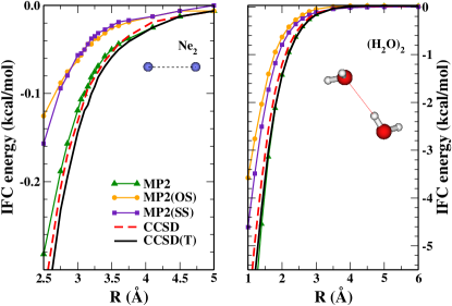
Figure 1: Inter–fragment correlation (IFC) energy of Ne₂ and (H₂O)₂ as computed with different methods.

It can be observed that for noncovalent interactions, with good approximation, the IFC energies computed at the MP2 (or equivalently MP2(SS) or MP2(OS)) level and at the CCSD(T) level are proportional to each other over a wide range of inter–fragment distances $R$. This proportionality can be verified by direct comparison of the IFC energies calculated at different levels of theory for various noncovalent interacting complexes (see Fig. 2).

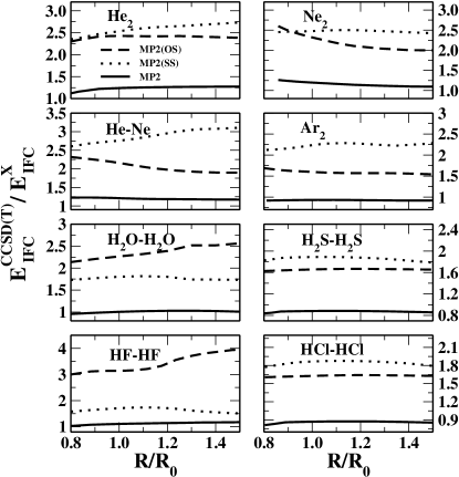
Figure 2: Ratio between different spin–resolved MP2 IFC energies and CCSD(T) ones, for various systems at several distances. $R_{0}$ denotes the equilibrium distance of each complex. $X$ = MP2 [continuous line], MP2(OS) [dashed line], and MP2(SS) [dotted line].

For MP2 the proportionality is very well satisfied for all systems and distances. MP2(SS) and MP2(OS) show instead some larger deviations at higher distances. However such deviations are not very relevant, because the IFC energy is rapidly approaching zero for large distances. In fact, as shown in Fig. 1, for $R/R_{0}\gtrsim$1.5 the IFC is already close or below subchemical accuracy.

The proportionality of the (spin–resolved) MP2 and coupled cluster energies can be rationalized considering that in noncovalent complexes the variation of IFC with distance is mainly due to relaxation of intramolecular contributions, thus both MP2 and CCSD(T) IFC energies display a very similar behavior with $R$ and their ratio stays almost constant.

This proportionality can be used to define single–parameter scaled (spin–resolved) MP2 approaches suitable for the description of the dissociation of noncovalent complexes. To do that, we define

$$E_{IFC}^{\mathrm{S(R)-MP2}} = c_{S}E_{IFC}^{\mathrm{MP2}}$$ (5)

$$E_{IFC}^{\mathrm{SOS(R)-MP2}} = c_{OS}E_{IFC}^{\mathrm{MP2(OS)}}$$ (6)

$$E_{IFC}^{\mathrm{SSS(R)-MP2}} = c_{SS}E_{IFC}^{\mathrm{MP2(SS)}}\ ,$$ (7)

with

$$c_{S} = \frac{E_{IFC}^{\mathrm{CCSD(T)}}(\tilde{R})}{E_{IFC}^{MP2}(\tilde{R})}$$ (8)

$$c_{OS} = \frac{E_{IFC}^{\mathrm{CCSD(T)}}(\tilde{R})}{E_{IFC}^{MP2(OS)}(\tilde{R})}$$ (9)

$$c_{SS} = \frac{E_{IFC}^{\mathrm{CCSD(T)}}(\tilde{R})}{E_{IFC}^{MP2(SS)}(\tilde{R})}$$ (10)

where $\tilde{R}$ is some reference distance. With this definition we fix (at the cost of a single expensive CCSD(T) calculation) the proportionality between (spin–resolved) MP2 and CCSD(T) results, by simply imposing that at some point, the two IFC energies, or analogously, the respective total binding energies ($E_{b}$) are the same.

The choice of the reference point $\tilde{R}$ in Eqs. (8)–(10) is not a major concern, since the value of $c$ is almost independent on it (see Fig. 2 and subsection III.1). In this work we have chosen for the the reference point the equilibrium distance $R_{0}$, computed at the CCSD(T) level. This choice is not mandatory, nevertheless it appears the best compromise between the need to avoid too short distances (where the proportionality relation may be less accurate) and the necessity to avoid the use of too small energies (as would result for large $R$ values) in the ratio of Eqs. (8)–(10) to minimize numerical noise(see subsection III.1 for a further discussion).

Each of the equations (8), (9), (10) provides a simple non–empirical procedure for fixing the (system–dependent) scaling factor in one–parameter (SCS–)MP2 calculations when dissociation energies of noncovalent systems are of interest. Thus, a whole dissociation curve, comprising many single–point results, can be simulated by performing only a single CCSD(T) calculation and without the introduction of any empirical parameter.

The main question is if the accuracy of the such procedure is high enough. In section III we will show that deviations from the CCSD(T) reference results are indeed well below subchemical accuracy (i.e. 0.1 kcal/mol).

II.1 Computational details

To test our scaling approach we considered a representative set of small noncovalently interacting systems: He₂, Ne₂, He–Ne, Ar₂ (dispersion interaction), (H₂O)₂, (HF)₂ (hydrogen bond), (H₂S)₂, (HCl)₂ (dipole–dipole interaction). Additionally, benzene–HCN, the stacked benzene dimer, and Be₂ have been also considered, as particular cases. The former two are in fact relatively large systems with the first one also displaying a mixed electrostatic–dispersion character, which changes with the bond distance Gráfová et al. (2010). The latter is a system where MP2 and CCSD completely fail even qualitatively Schmidt et al. (2010). The sizes of the molecules included in our test set were limited by the need to compute in all cases the full CCSD(T) dissociation curves for reference purposes, except for benzene–HCN and the stacked benzene dimer in which case the reference data were taken from Ref. Gráfová et al. (2010).

Calculations were performed with the ACES II Stanton et al. (2007) and TURBOMOLE TUR program packages. For all systems an aug–cc–pVQZ basis set Dunning, Jr. (1989); Woon and Dunning, Jr. (1994, 1993) was used, except for Ne₂ (uncontracted aug–cc–pVTZ), Be₂ (cc–pV5Z), and Ar₂ (aug–cc–pV5Z).

To assess the performance of the different methods to reproduce the full dissociation curves we considered the mean absolute error:

$$\mathrm{MAE}(X)=\frac{1}{R_{max}-R_{0}}\int_{R_{0}}^{R_{max}}|\Delta E^{X}(R)|dR\ ,$$ (11)

where $X$=CCSD, MP2, SOS(R)–MP2, …, and

$$\Delta E^{X}(R)\equiv E_{IFC}^{X}(R)-E_{IFC}^{CCSD(T)}(R)\ .$$ (12)

Note that because all the methods considered here use the Hartree–Fock exchange, the difference between the IFC energies of different methods in Eq. (12) are exactly the same as the differences in the total interaction energies. The MAE$(X)$ defined in Eq. (11) measures the average deviation of the results from the reference CCSD(T) data over a given interval. In our work we decided to remove from this evaluation the smallest values of $R$, because our approach might be not fully justified at such small inter–fragment distances. Hence, the lower bound for the integration was fixed at $R_{0}$. The upper bound of the integral was fixed instead to the value of $R$ beyond which the CCSD(T) IFC energy is lower than 10^-4 Hartree, in order to keep the normalization factor finite in Eq. (11).

Finally, we note that in all calculations no correction for the basis set superposition error (BSSE) was included, for computational simplicity and because it is readsorbed in the scaling coefficient. For the water dimer, e.g., we check that, including a BSSE correction, the MAE of Eq. (11) is 36.7, 36.6 , 5.5 $10^{-3}$ kcal/mol, for SOS(R)-MP2, SSS(R)-MP2 and S(R)-MP2 respectively. These values are in good agreement with the ones (without BSSE) reported in Tab. 2.

III Results

The values of the $c_{S}$, $c_{OS}$, and $c_{SS}$ coefficients, obtained by applying Eqs. (8), (9), and (10) to the systems considered in this work, are reported in Table 1, together with the reference inter–fragment separation $R_{0}$.

Table 1: Values of the $c_{OS}$, $c_{SS}$, and $c_{S}$ coefficients obtained via Eqs. (8), (9), (10) calculated at distance $R_{0}$ for all the systems presented in this paper.

system		$c_{OS}$	$c_{SS}$	$c_{S}$		$R_{0}$[Å]
He2		2.43	2.53	1.24		3.0
He–Ne		2.15	2.76	1.21		3.0
Ne2		2.34	2.47	1.20		3.2
Ar2		1.60	2.24	0.93		3.7
H2S–H2S		1.66	1.89	0.88		2.8
HCl–HCl		1.63	1.87	0.87		2.5
HF–HF		3.14	1.71	1.11		1.8
H2O–H2O		2.27	1.80	1.00		2.0

Inspection of the table confirms that the optimal scaling coefficients for (spin–resolved) MP2 calculations are significantly system dependent. This dependence is also more pronounced for the SSS(R)–MP2 method, in which MP2(SS) includes only a small part of the total correlation contribution, while it is much weaker for MP2, which can describe better the whole correlation effects. It is interesting to note, in addition, that the variation of the scaling coefficients among different systems is not the same for the various methods. In fact, for example the $c_{OS}$ is maximum for HF–HF and almost twice as big as the $c_{OS}$ for Ar₂, while the value of $c_{SS}$ for HF–HF is about 20% smaller than the Ar₂ one and it is maximum for He–Ne. Therefore, no clear trend can be identified for the values of the scaling coefficients when different systems (and methods) are considered.

The results of Tab. 1 also indicate that, due to the variability of the optimal scaling coefficients, global scaling factors can hardly be expected to achieve high accuracy for a broad range of applications. In fact, even if most of the coefficients displayed in the table agree reasonably well with the SOS(MI)–MP2 ($c_{OS(MI)}\approx 1.8$) and SSS(MI)–MP2 ($c_{SS(MI)}\approx 1.75$) values Hill and Platts (2007); Distasio Jr. and Head-Gordon (2007), which were especially optimized for intermolecular interaction energies, some remarkable differences appear. These reflect the peculiarities of the correlation in some systems (e.g. same–spin correlation in He₂ or opposite–spin correlation in HF–HF) which cannot be captured by “average” scaling procedures. Note finally, that all the $c_{OS}$ values are rather different from the conventional scaling coefficient of 1.3 proposed for quantum chemical applications Jung et al. (2004).

To demonstrate the performance of the method we report in Fig. 3 the binding energies of two dispersion dimers (He₂ and Ne₂) as computed with different methods.

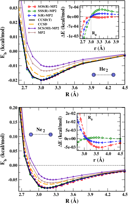
Figure 3: Binding energy of He₂ and Ne₂ as computed with different theoretical methods. In the insets we report the difference between S(R)–MP2, SSS(R)–MP2, SOS(R)–MP2 and CCSD(T) inter–fragment correlation energies (see Eq. (12)). $R_{0}$ denotes the equilibrium distance.

The figure shows that the proposed scaled–(spin–resolved)–MP2 approaches yield very good results, giving binding energy curves which are almost indistinguishable form the reference CCSD(T) ones over the whole range of inter–atomic distances considered. On the contrary, visible differences with the reference are found by considering CCSD, MP2, and SCS(MI)–MP2 results. To have more insight into these results we show in the insets of Fig. 3 also the differences between our S(R)–MP2, SOS(R)–MP2, and SSS(R)–MP2 and the CCSD(T) reference ($\Delta E$, Eq. (12)) at various distances. By definition all our approaches coincide with CCSD(T) at the equilibrium (reference) distance $R_{0}$. Remarkably, however, the accuracy of the method is found to be very good at any distance, in particular for $R>R_{0}$, where deviations from CCSD(T) values are vanishing small (of the order of 10^-3 kcal/mol). Such accuracy is not only well below subchemical accuracy but also largely sufficient to yield a highly accurate description of these dispersion dimers, as demonstrated by the comparison of the binding energy curves.

As further examples Fig. 4 reports the $\Delta E$ values also for one hydrogen–bond complex (H₂O dimer) and one dipole–dipole complex (H₂S dimer). In this case the binding curves are instead not reported because due to the relatively large value of $E_{b}$ the differences between the different methods are not easily visible on that scale.

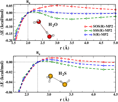
Figure 4: The difference ($\Delta E$, see Eq. (12)) between S(R)–MP2, SSS(R)–MP2, SOS(R)–MP2 and CCSD(T) inter–fragment correlation energies calculated for (H₂O)₂ and (H₂S)₂. $R_{0}$ denotes the equilibrium distance.

Inspection of the figure shows again that the present scaled approaches provide very accurate IFC energies over a broad range of intermolecular distances, with discrepancies from the reference well below the subchemical accuracy. The analysis of these results, together with those of Figs. 2 and 3, indicates that the S(R)–MP2 approach is overall slightly more accurate than SOS(R)–MP2 and SSS(R)–MP2, but all yield highly accurate results. For short distances, however, the methods necessarily face some limitations. In fact, as we mentioned above, at short inter–system separations the proportionality relation between (spin–resolved) MP2 and CCSD(T) may deteriorate due to the raising importance of intermolecular correlation (that is, the direct interaction of electrons and pairs “localized” on different systems, starts to be relevant). Moreover, even in absence of this phenomenon, i.e. for systems and distances $R<R_{0}$ where Fig. 2 suggests that the proportionality holds, the values of $\Delta E$ may be expected to rapidly increase (in absolute values) as the IFC energy is very large for $R<R_{0}$, so that small deviations are largely magnified.

To have a more quantitative and global assessment of the quality of the scaling coefficients calculated within our simple non–empirical scaling scheme we report in Tab. 2 the mean absolute error, computed via Eq. (11), for several test systems and various methods, including the spin–component scaled methods optimized for intermolecular interactions Distasio Jr. and Head-Gordon (2007), the conventional SOS–MP2 with $c_{OS}=1.3$, the unscaled CCSD and empirical $1/R^{6}$, $1/R^{5}$, and Lennard–Jones (LJ) potentials (fixed by fitting to CCSD(T) at $R_{0}$). Moreover, for comparison, we report the MAEs obtained by the popular PBE-D3 density functional (PBE exchange-correlation functional Perdew et al. (1996) supplemented with the D3 empirical dispersion correction Grimme et al. (2010); note that the PBE functional is one of the best generalized gradient approximations for non–covalent interactions Burns et al. (2001); Fabiano et al. (2011)). For DFT calculation the MAEs were computed by considering $E_{b}$ in place of $E_{IFC}$ into Eq. (12).

Table 2: Mean absolute error, as defined in Eq. (11), for different methods. Binding energies (E_b) are in kcal/mol, other results are in 10^-3 kcal/mol. RMAE (Eq. (13)) is also reported in the last line.

System	Eb	SOS(R)	SSS(R)	S(R)	SCS(MI)	SOS(MI)	SSS(MI)	SOSa	$1/R^{6}$	$1/R^{5}$	LJ	PBE-D3b	CCSD
		–MP2
He–He	0.02	0.0	0.3	0.1	3.0	2.4	3.2	4.5	0.3	2.0	5.3	1.3	0.7
He–Ne	0.05	2.0	1.4	0.5	11.5	3.7	13.2	12.2	1.0	4.1	16.6	1.9	2.8
Ne–Ne	0.08	3.0	0.3	1.5	9.6	5.8	10.4	14.3	1.7	4.0	15.2	6.5	4.3
Ar–Ar	0.56	3.8	3.6	1.0	40.9	38.3	57.5	45.0	10.6	51.0	136.9	95.4	24.9
H2S–H2S	1.97	3.3	9.0	4.5	23.9	61.7	40.3	151.2	123.3	29.6	167.6	160.3	110.1
HCl–HCl	2.41	2.7	9.2	5.3	17.6	65.0	33.2	123.9	116.1	29.0	139.2	133.7	89.3
HF–HF	4.88	78.4	36.7	5.4	29.2	112.3	40.1	125.3	54.1	51.1	74.1	169.8	30.3
H2O–H2O	5.22	31.9	28.5	5.9	25.1	57.5	29.6	86.2	48.7	41.9	62.9	101.9	29.8
RMAE		1.37%	0.93%	0.53%	7.54%	5.34%	8.81%	11.23%	2.58%	4.61%	15.02%	6.82%	3.68%

a) Conventional SOS–MP2 with $c_{os}=1.3$.

b) These data were obtained by substituting $E_{IFC}$ with $E_{b}$ in Eq. (12).

The values in the table are all very small, and are reported in unit of 10^-3 kcal/mol. The first column reports the binding energy computed at the CCSD(T) level: the considered systems span a wide range of intermolecular forces. In the last line also the relative mean absolute error (RMAE) is reported, which is computed as:

$$\mathrm{RMAE}(X)=\frac{1}{N}\sum_{i}^{N}\frac{\mathrm{MAE}_{i}(X)}{E_{b}[i]}\,$$ (13)

where the sum runs over all the $N$ systems and $E_{b}[i]$ is the binding energy of the $i$-th complex. The RMAE allows a fair global assessment of all the results.

The results of Tab. 2 clearly show that the MP2–based methods using the here proposed non–empirical scaling can reproduce the reference CCSD(T) results with an accuracy below $1.5\%$ in all systems (with a maximum MAE of 0.078 kcal/mol), with an accuracy two–three times better than the CCSD method (RMAE=3.68%). In particular, the present S(R)–MP2 has the lowest RMAE (0.53%) confirming its very high accuracy (the S(R)–MP2 MAE is always extremely small, lower than 0.006 kcal/mol). On the other hand, SCS(MI)–, SOS(MI)–, and SSS(MI)–MP2, despite performing very well in absolute terms (the deviation from CCSD(T) ranges from 0.003 to 0.1 kcal/mol) yield significantly worse results, with RMAE larger than $5\%$.

A relatively small RMAE is obtained by the empirical $1/R^{6}$ fit. This result however depends on the fact that in our test set simple dispersion dimers are predominant. The empirical potential works however much worse for other cases. In any case the RMAE of the $1/R^{6}$ fit is five times worse than that of the S(R)–MP2 approach.

Finally, the PBE-D3 approach works fairly well, yielding a RMAE comparable to that of the SOS(MI)– and SCS(MI)–MP2 methods, but in any case more than five times larger than all the methods using the here proposed non–empirical scaling procedure. In addition, we note that the PBE-D3 method yields very good results for dispersion dimers, but not so good accuracy for hydrogen-bond and dipole-dipole complexes.

III.1 Role of the reference distance

In this subsection we shortly analyze the role of the reference distance used to compute the scaling coefficients in Eqs. (8), (9), and (10). To this end we report in Tab. 3 the relative variation of the scaling coefficients and the MAEs (Eq. (11)) when the reference distance is changed from the equilibrium value $R_{0}$ to $\tilde{R}>R_{0}$.

Table 3: Relative values (with respect to equilibrium geometry) of the scaling coefficients (obtained via Eq. (8)) and mean absolute errors (Eq. (11)) calculated at non equilibrium distances ($\tilde{R}>R_{0}$) for all the systems presented in this paper.

					Mean absolute error
System	$\tilde{R}$	$c_{OS}$	$c_{SS}$	$c_{S}$	SOS(R)–MP2	SSS(R)–MP2	S(R)–MP2
He2	1.1	1.00	1.00	1.00	1.00	0.67	1.00
Ne2	1.1	0.95	1.01	0.98	0.60	0.67	0.67
He–Ne	1.1	0.95	1.04	0.98	0.55	0.71	0.40
Ar2	1.1	0.99	1.02	1.00	0.47	0.64	1.10
H2O–H2O	1.3	1.11	0.97	1.03	0.96	1.06	0.90
HF–HF	1.3	1.13	0.99	1.04	1.17	1.01	0.85
H2S–H2S	1.2	1.01	1.00	1.00	0.67	0.99	1.07
HCl–HCl	1.2	1.01	1.00	1.00	0.85	1.00	1.00

The tabulated results show that scaling coefficients change very little, as can be already inferred from Fig. 2. This provides a validation of the working hypothesis and indicates the robustness of our simple non–empirical scaling procedure. By inspecting the relative MAEs reported in Tab. 3 we see that the accuracy of the methods is not only preserved but in many cases is also improved. The improvement is anyway rather small and can be considered to lay within the numerical uncertainty related to the definition of the MAE (Eq. (11)).

This result is important because it remarks the possibility to utilize the present non–empirical scaling procedure also in all those cases where the equilibrium distance is not known, by simply performing a single CCSD(T) calculations at any “reasonable” bond distance.

III.2 Benzene complexes

In this subsection we consider the application of our new scaling method to larger systems, namely the benzene–HCN T–shaped complex and the stacked benzene dimer.

The first of these systems is particularly interesting because the interaction has a mixed character involving both electrostatic and dispersion contributions in a variable proportion along the dissociation curve Gráfová et al. (2010). Its dissociation curves computed at the (spin–resolved) MP2 level as well as the corresponding scaled results are reported in Fig. 5. Reference CCSD(T) data from Ref. Gráfová et al. (2010) are also reported.

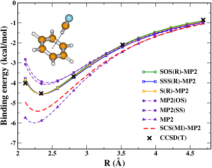
Figure 5: Binding energy for the benzene–HCN complex as a function of the inter–atomic distance $R$, for different methods.

The scaling coefficients have been computed at the equilibrium distance of 2.34 Å and are $c_{OS}=1.27$, $c_{SS}=1.35$, and $c_{S}=0.66$.

Consistently with the results discussed in the main body of section III, the non–empirical scaling methods all perform remarkably well, substantially improving over “bare” MP2, MP2(OS), and MP2(SS) calculations and especially over empirically scaling methods (e.g. SCS(MI)–MP2). S(R)–MP2, SOS(R)–MP2 and SSS(R)–MP2 show in fact deviations from the reference data below 0.5 kcal/mol along the whole range of distances considered.

Similar results are found also by using scaling coefficients obtained considering a different reference distance $\tilde{R}$. For $\tilde{R}=2.81$Å, indeed, we found $c_{OS}$=1.15, $c_{SS}$=1.14, $c_{S}$=0.57, and essentially the same performance for the binding energy (or equivalently the IFC energy). In fact, the scaling coefficients computed at the new distance are in good agreement, although slightly smaller, with the ones computed at the equilibrium distance. We remark that the small difference between the coefficients computed at different reference distances shall, in this special case, be partially traced back to the computational noise originating from the fact that the reference CCSD(T) values were not computed with the same set up as the MP2 ones, but rather extracted from the total binding energies (HF+CCSD(T) at the CBS limit) reported in Ref. Gráfová et al. (2010). Despite this small issue, the non–empirically scaled methods display an impressive robustness.

As a further test we consider a typical $\pi$-stacking complex. In Fig. 6 we thus report the dissociation curve of the stacked benzene dimer as computed at the (spin–resolved) MP2 level and with the various scaled approaches. Reference CCSD(T) data from Ref. Gráfová et al. (2010) are also reported. The scaling coefficients have been computed at the equilibrium distance of 3.765 Å and are $c_{OS}=1.39$, $c_{SS}=1.66$, and $c_{S}=0.76$.

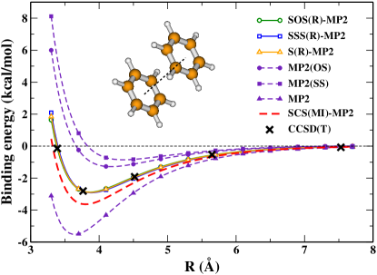
Figure 6: Binding energy for the stacked benzene dimer as a function of the inter–atomic distance $R$, for different methods.

Inspection of the figure shows that, similarly with the case of the benzene-HCN complex, all the scaled methods perform remarkably well yielding deviations within 0.2 kcal/mol from the reference CCSD(T) data. In particular, the non–empirical scaling procedure proposed here demonstrates to be able to correct well both the overbinding of the MP2 method and the strong underbinding of the MP2(OS) and MP2(SS) approaches.

Overall, the dissociation curves computed with our scaling approach agree very well with reference data and show that the method is very effective even for such “large” and “difficult” systems as the present ones. We note that this performance is remarkable especially for SOS(R)– and SSS(R)–MP2, because the MP2(OS) and MP2(SS) binding energies are almost degenerate, so that the corresponding scaling coefficient are almost identical. Thus, the same scaling is obtained for the two methods. However, this has only a minor effect on the SSS(R)–MP2 results at relatively small distances, while a good performance is observed for bond distances larger than the equilibrium one. This shows once more that the here presented scaling procedure is rather robust in many different situations.

III.3 Beryllium dimer

Finally, we consider in Fig. 7 the Beryllium dimer, which is a very difficult system where MP2 and CCSD fail to give even an approximate quantitative description of the dissociation curve Schmidt et al. (2010). For this system even CCSD(T) shows some limitations Schmidt et al. (2010). However, this high-level method can at least capture most of the features of the dissociation curve. Therefore, it will be used anyway as reference in the present example, although caution must be paid to the quantitative analysis of the results.

In this case, the computed scaling coefficients are $c_{OS}=1.79$, $c_{SS}=3.03$, and $c_{S}=1.13$. However, an accurate description of the dissociation curve is found only using the SOS(R)–MP2 method. On the contrary, methods based on the same–spin correlation fail quite evidently. This may be due to the fact that in this system, where static correlation is important, the stretching of the bond is not only promoting polarization and induction phenomena in each atom, but is also changing the actual “multireference” description of the system, influencing the same–spin correlation which includes antisymmetrized integrals. This fact indicates that the use of MP2(SS) correlation energy in scaling procedures has strong limitations for this peculiar system. Due to this limitations also the S(R)–MP2 method, which includes important contributions of same–spin correlation, cannot be accurate. Nevertheless, we remark that S(R)–MP2 and even SSS(R)–MP2 can compensate the limitations of the underlying MP2(SS) energy relatively well, thanks to appropriate values of the scaling factor granted by Eqs. (8), (9), (10). However, the independence of the scaling factor from the reference separation is partially lost and only a limited portion of the dissociation curve can be properly described when same–spin correlation is considered.

The SOS(R)–MP2 method with coefficients calculated in our scaled procedure provides for the Be₂ the best dissociation curve (as compared to CCSD(T)) significantly outperforming MP2, CCSD or SOS(MI)–MP2 methods.

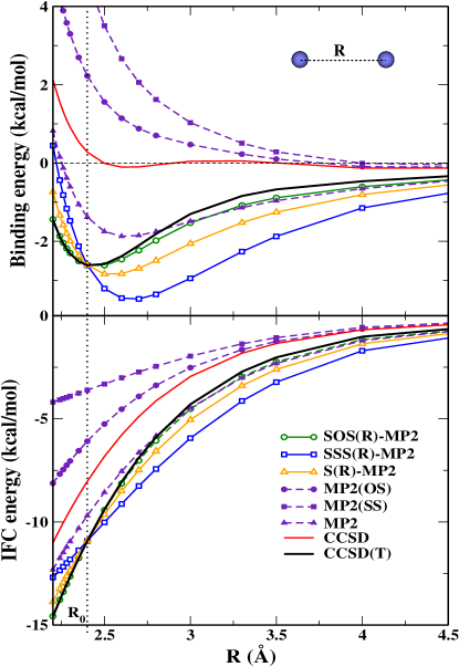
Figure 7: Binding energy and IFC energy for Be₂ as a function of the inter–atomic distance $R$, for different methods. $R_{0}$ denotes the equilibrium distance.

IV Conclusions

We have proposed a simple non–empirical procedure which can be used to calculate optimal scaling coefficients for (spin–resolved) MP2 calculations of the dissociation of noncovalent complexes. The applicability of the proposed method was demonstrated for a series of test systems, considering equilibrium and non–equilibrium reference distances, as well as for a notoriously difficult case as Be₂. The obtained results show that the presented method works well in most cases, confirming the robustness of our hypothesis.

The proposed method is especially attractive because it allows to obtain a full dissociation curve of almost CCSD(T) quality at the cost of just a single CCSD(T) calculation. Moreover, it is conceivable to replace the costly CCSD(T) calculation with a focal–point analysis East and Allen (1993); Csaszar et al. (1998) (the $\Delta$CCSD(T) procedure) to obtain an estimate of the CCSD(T) correlation energy from a cheaper calculation. In this way the computational cost is much reduced, losing only little on accuracy. Thus, future applications on large systems can be foreseen. Moreover, it might be also possible to replace the CCSD(T) reference with an alternative accurate treatment of the correlation, e.g. the CCSD[T] Urban et al. (1986); Řezáč et al. (2013) or the FNO CCSD(T) A. E. DePrince and Sherrill (2013) method, to optimize the accuracy or the computational effort.

Finally we remark that, although in this paper we focused only on single–parameter scaled MP2 methods, the methodology presented here can be extended in the future to treat the more general case of spin–component–scaled (SCS) MP2 calculations with two parameters ($c_{OS}$ and $c_{SS}$). To this end Eqs. (5)-(7) will be generalized to

$$E_{IFC}^{\mathrm{CCSD(T)}}(\tilde{R})=c_{OS}E_{IFC}^{MP2(OS)}(\tilde{R})+c_{SS}E_{IFC}^{MP2(SS)}(\tilde{R})\;,$$ (14)

and an additional constraint will be needed for the scaling parameters (e.g. fixing the sum or the ratio of the parameters from theoretical considerations). We also have to stress that this approach can be useful for the verification of the quality of SCS coefficients used in different SCS–MP2 methods.

Acknowledgments This work was supported by the Polish Committee for Scientific Research MNiSW under Grant no. N N204 560839 and by the ERC–StG FP7 Project DEDOM (no. 207441). We thank TURBOMOLE GmbH for providing the TURBOMOLE program package and M. Margarito for technical support.

References

- Hobza and Müller-Dethlefs (2010) P. Hobza and K. Müller-Dethlefs, Noncovalent Interactions: Theory and Experiment (The Royal Society of Chemistry, Cambridge, 2010).
- Raghavachari et al. (1989) K. Raghavachari, G. W. Trucks, J. A. Pople, and M. Head-Gordon, Chem. Phys. Lett. 157, 479 (1989).
- Hobza (2012) P. Hobza, Acc. Chem. Res. 45, 663 (2012).
- Zhao and Truhlar (2005) Y. Zhao and D. G. Truhlar, J. Chem. Theory Comput. 1, 415 (2005).
- Zhao and Truhlar (2006) Y. Zhao and D. G. Truhlar, J. Chem. Theory Comput. 2, 1009 (2006).
- Riley et al. (2010) K. E. Riley, M. Pitoňák, P. Jurečka, and P. Hobza, Chem. Rev. 110, 5023 (2010).
- Riley et al. (2012) K. E. Riley, J. A. Platts, J. Řezáč, P. Hobza, and J. G. Hill, J. Phys. Chem. A 116, 4159 (2012).
- Marshall et al. (2001) M. S. Marshall, L. A. Burns, and C. D. Sherrill, J. Chem. Phys. 135, 194102 (2001).
- Grimme (2003) S. Grimme, J. Chem. Phys. 118, 9095 (2003).
- Grimme et al. (2012) S. Grimme, L. Goerigk, and R. F. Fink, Wiley Interdisciplinary Reviews: Computational Molecular Science 2, 886 (2012), ISSN 1759-0884, URL http://dx.doi.org/10.1002/wcms.1110.
- Distasio Jr. and Head-Gordon (2007) R. A. Distasio Jr. and M. Head-Gordon, Mol. Phys. 105, 1073 (2007).
- Hill and Platts (2007) J. G. Hill and J. A. Platts, J. Chem. Theory Comput. 3, 80 (2007).
- Jung et al. (2004) Y. Jung, R. C. Lochan, A. D. Dutoi, and M. Head-Gordon, J. Chem. Phys. 121, 9793 (2004).
- Lochan et al. (2005) R. C. Lochan, Y. Jung, and M. Head-Gordon, J. Phys. Chem. A 109, 7598 (2005).
- Szabados (2006) A. Szabados, J. Chem. Phys. 125, 214105 (2006).
- Fink (2010) R. F. Fink, J. Chem. Phys. 133, 174113 (2010).
- Usvyat et al. (2012) D. Usvyat, K. Sadeghian, L. Maschio, and M. Schütz, Phys. Rev. B 86, 045412 (2012), URL http://link.aps.org/doi/10.1103/PhysRevB.86.045412.
- Gráfová et al. (2010) L. Gráfová, M. Pitoňák, J. Řezáč, and P. Hobza, J. Chem. Theory Comput. 6, 2365 (2010).
- Schmidt et al. (2010) M. W. Schmidt, J. Ivanic, and K. Ruedenberg, J. Phys. Chem. A 114, 8687 (2010).
- Stanton et al. (2007) J. F. Stanton, J. Gauss, J. D. Watts, M. Nooijen, N. Oliphant, S. A. Perera, P. Szalay, W. J. Lauderdale, S. Kucharski, S. Gwaltney, et al., ACES II (Quantum Theory Project, Gainesville, Florida, 2007).
- (21) TURBOMOLE V6.4 2012, a development of University of Karlsruhe and Forschungszentrum Karlsruhe GmbH, 1989-2007, TURBOMOLE GmbH, since 2007; available from http://www.turbomole.com.
- Dunning, Jr. (1989) T. H. Dunning, Jr., J. Chem. Phys. 90, 1007 (1989).
- Woon and Dunning, Jr. (1994) D. E. Woon and T. H. Dunning, Jr., J. Chem. Phys. 100, 2975 (1994).
- Woon and Dunning, Jr. (1993) D. E. Woon and T. H. Dunning, Jr., J. Chem. Phys. 98, 1358 (1993).
- Perdew et al. (1996) J. P. Perdew, K. Burke, and M. Ernzerhof, Phys. Rev. Lett. 77, 3865 (1996).
- Grimme et al. (2010) S. Grimme, J. Antony, S. Ehrlich, and H. Krieg, J. Chem. Phys. 132, 154104 (2010).
- Burns et al. (2001) L. A. Burns, A. Vázquez-Mayagoitia, B. G. Sumpter, and C. D. Sherrill, J. Chem. Phys. 134, 084107 (2001).
- Fabiano et al. (2011) E. Fabiano, L. A. Constantin, and F. Della Sala, J. Chem. Theory Comput. 7, 3548 (2011).
- East and Allen (1993) A. L. L. East and W. D. Allen, J. Chem. Phys. 99, 4638 (1993).
- Csaszar et al. (1998) A. G. Csaszar, W. D. Allen, and H. F. Schaefer, J. Chem. Phys. 108, 9571 (1998).
- Urban et al. (1986) M. Urban, J. Noga, J. Cole, and R. J. Bartlett, J. Phys. Chem. 83, 4041 (1986).
- Řezáč et al. (2013) J. Řezáč, L. Šimoňa, and P. Hobza, J. Chem. Theory Comput. 9, 364 (2013).
- A. E. DePrince and Sherrill (2013) I. A. E. DePrince and C. D. Sherrill, J. Chem. Theory Comput. 9, 293 (2013).