The modellers’ encounter with ecological theory. Or, what is this thing called ‘growth rate’?

Abstract

The attempt to determine the population growth rate from field data reveals several ambiguities in its definition(s), which seem to throw into question the very concept itself. However, an alternative point of view is proposed that not only preserves the identity of the concept, but also helps discriminate between competing models for capturing the data.

Introduction

Imagine a group of quantitative scientists, such as statisticians or mathematicians, with only a textbook knowledge of ecology, who are charged with analyzing a dataset of population counts. Let us call these scientists the “Modellers”. The Modellers feel that if their analysis is to be relevant to ecologists, it should relate to what they understand to be the most important notion in population ecology, the population growth rate. This note is written from the perspective of the Modellers and describes the difficulties they experience in the process, as well as their attempts at overcoming them.

What is the growth rate?

We give just one piece of evidence of the fundamental importance of the growth rate by quoting Berryman (2003) [1] who makes it the unsung hero of a fundamental law of ecology:

The first principle (geometric growth)
Ecologists seem to agree, in general, that geometric (exponential) growth is a good candidate for a law of population ecology. […] since geometric growth is a fundamental and self-evident property of all populations living under a certain set of conditions (unlimited resources), I prefer to think of it as the first founding principle of population dynamics […]

We have no intention here to enter the fray of the extensive debate among ecologists about whether Berryman’s law (a.k.a. the Malthusian Law) is in fact a Law of Nature and/or whether ecology has any laws at all; although we admit that the title of O’Hara’s spirited article [16] on the subject provided some inspiration for the title of the present paper.

Rather, we imagine the Modellers taking Berryman’s law to be thedefinition of the growth rate, according to which it is simply the number $r$ in an exponential-growth expression of the form $N\sim e^{rt}$ (or the discrete-time version thereof), where $N=N(t)$ denotes the total number of individuals at time $t$. As a result, the existence of a well-defined growth rate is contingent on populations under the condition of “unlimited resources" following an exponential growth law.

But then, what about the Modellers’ data, which are shown in Fig. 1 below?

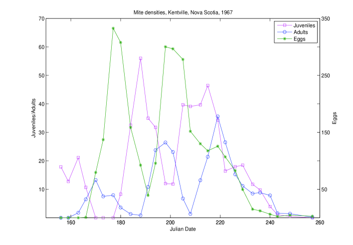
Figure 1: Mite-population field data (note the different scales for juveniles/adults and eggs).

This is a plot of field data of mites on apple trees, which, at least at the beginning of the season, do not experience any significant resource limitation. So what are the Modellers to make of the large oscillations? This does not look like a simple exponential $e^{rt}$ at all — at least not as long as $r$ is a real number; and which ecologist would put up with a complex growth rate?

One, two, three growth rates?

The Modellers may start over and look for the standard definition, which, in the words of e.g. Sibly and Hone (2002) [20], reads

Population growth rate describes the per capita rate of growth of a population, either as the factor by which population size increases per year, conventionally given the symbol $\lambda(=N_{t+1}/N_{t})$, or as $r=\log\lambda$.

But when this definition is applied to the data shown in Fig. 1 (mutatis mutandis; the relevant time step is obviously not a year) the growth rate “suddenly" starts fluctuating wildly between positive and negative values (Fig. 2).

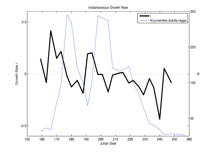
Figure 2: Instantaneous growth rate $r=\log\left(N(t+\Delta t)/N(t)\right)$, where $N(t)=E(t)+J(t)+A(t)$ is the total number of individuals.

Does this mean that a constant growth rate does not exist after all? Even if the environmental conditions are constant (as they are – at least approximately – during the beginning of the mite season)?

Sibly and Hone continue as one would expect from textbook ecology.

In the simplest population model all individuals in the population are assumed equivalent, with the same death rates and birth rates, and there is no migration in or out of the population, so exponential growth occurs; in this model, population growth rate = $r$ = instantaneous birth rate – instantaneous death rate.

What interests us the most in this quote is the appearance of the term “model" in the description of the growth rate, but more on this later. For now, we read on a little further:

Population growth rate is typically estimated using either census data over time or from demographic (fecundity and survival) data. Census data are analysed by the linear regression of the natural logarithms of abundance over time, and demographic data using the Euler–Lotka equation (Caughley 1977) and population projection matrices (Caswell 2001).

So here it is: according to this, there are at least two kinds of growth rates: one based on “demographic data", and one based on “census data". Moreover, the former seems to draw in other quantities (“fecundity and survival"), which seem to have to be known independently/beforehand.

But, if the growth rate is an inherent property of a population, should it not manifest itself in a measured population curve? Should it not be possible to determine it from measured data without reference to outside information? This appears to discredit the demographic variant of the concept – or maybe the demographic calculation as described gives an ecological quantity that is different from the growth rate.

What is more, Sibly and Hone also give two ways of “analysing" census data. In the first quote above, they present the simple formula $r=\log\left(N_{t+1}/N_{t}\right)$; i.e., the formula for the “instantaneous" growth rate [24]. Now they suggest to use “linear regression of the natural logarithms of abundance over time”, which will result in an averaged or smoothed growth quantity. But will the numerical value(s) depend on the time interval(s)? If the Modellers are asked to take averages, how are they going to decide which time interval to use?

In any case, the supposedly fundamental (and elementary) concept of growth rate certainly seems to have lost some of its simplicity and clarity.

Asymptotic vs. transient growth rate (population structure)

Experienced ecologists will readily identify the large oscillations in the data of Fig. 1 as generational waves, and they will argue that in determining the growth rate one must account for the (st)age structure of the population.

The Modellers, obediently, consult e.g. Tenhumberg (2010) [22] who uses the (instantaneous) census-data definition of the growth rate, complete with its fluctuations during the early season (“transient dynamics"), and only offers them the piece of mind of a constant-value growth rate asymptotically.

If nothing else changes, the population eventually reaches the stable stage distribution and the speed at which the population is growing approaches a constant rate (the asymptotic population growth rate).

This, of course, refers to the mathematical fact, discovered by Lotka [14], that solutions to the appropriate demographic model for structured populations eventually settle on the stable age distribution and grow exponentially with a rate that can be computed from the demographic data (“Lotka’s r" or “intrinsic rate of increase" [24]). The census-data and demographic growth rates of Sibly and Hone are in this sense actually identical!

However, this is still unsatisfactory – at least for anyone ready to accept Berryman’s law: it is, in fact, precisely during the early season that resource limitations are the least likely to occur; so during this period the exponential-growth law should work particularly well. Having to wait until the stable age distribution is assumed seems counter-intuitive — as well as unrealistic and impractical, as many species will experience diminished growth due to limited resources before they can even approach the asymptotic state and/or will change their characteristics altogether due to seasonal behaviour etc. The Modellers’ field data exhibit evidence of both phenomena: the growth of the population slows down and comes to a halt after what appears to be 20-50 days; and during the final part of the season, the population crashes, as the mites switch to laying next–season eggs that will not hatch during the season they are laid (the egg numbers shown in Fig. 1 are for same-season eggs).

It is an interesting fact, which probably deserves to be better known, that classical demography itself offers a resolution of this conundrum. Properly “re-weighting” of the (st)age groups; i.e., considering

$$V(t):=\int_{0}^{\infty}v(a)\rho(t,a)da,$$

does indeed result in an exponential-growth law of the form $V(t)\sim e^{rt}$, where $r$ is the “asymptotic growth rate" in the parlance of Tenhumberg (i.e. Lotka’s $r$). The important point here is that the exponential–growth formula for the aggregate quantity $V(t)$ actually holds for all $t$, not just for large $t$, as Tenhumberg’s terminology suggests. Demographers know the function $v(a)$ to be Fisher’s [6] age-dependent reproductive value and $V(t)$ to be the total reproductive value. The resolution of the “early-season-vs.-asymptotic" conundrum, therefore, lies in the realization that only a very specific aggregate population-size quantity (namely $V(t)$) obeys the exponential-growth law stipulated by Berryman. Other quantities, such as the total number of individuals $N(t)=\int\rho(t,a)da$, will generally not grow according to a simple exponential.

	Time Window
Model	30 days	50 days	70 days
I
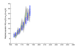
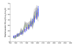
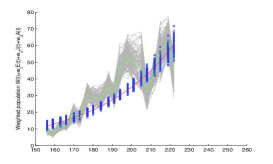
II

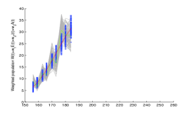
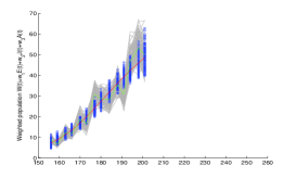
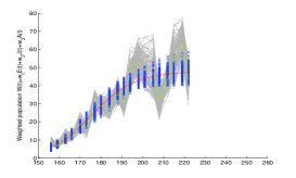
Figure 10: Fits of models I & II to re-weighted data $W(t)=w_{1}E(t)+w_{2}J(t)+w_{3}A(t)$. Plots analogous to 7. The reduction of the generational fluctuations is evident (see main text).

As an aside, it is amusing to see that applying a very simple, purely heuristic re-weighting formula of the form $W(t)=w_{1}E(t)+w_{2}J(t)+w_{3}A(t)$ can reduce the generational fluctuations in the data significantly, as demonstrated in Fig. 3 (as well as Figures 10 and 11 in E). Here the weights $w_{j}$ are computed by taking ratios of life-stage averages (see eq. (6)) and the step function

$$w(a):=\left\{\begin{array}[]{cl}w_{1},&\textrm{$a=$ egg age}\\ w_{2},&\textrm{$a=$ juvenile age}\\ w_{3},&\textrm{$a=$ adult age}\end{array}\right.$$

serves as a surrogate for $v(a)$.

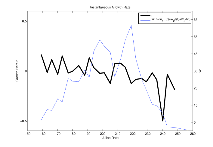
Figure 3: Instantaneous growth rate derived from the heuristically re-weighted aggregate population $W(t)=w_{1}E(t)+w_{2}J(t)+w_{3}A(t)$ (see text). Compared with Fig. 2, seasonal fluctuations during the growing phase of the season are reduced significantly.

Model parameters seasonal formula (SM) I simple exponential 2 no (1), $K=\infty$ II simple logistic 3 no (1) III linear phenomenological 11 yes (2a)–(2d), $K=\infty$ IV nonlinear phenomenological 12 yes (2a)–(2d) V linear demographic 10 yes (3a)–(3d), $\nu=0$ VI nonlinear demographic 11 yes (3a)–(3d)

Table 1: Models used. For details see B of the Supplementary Material (SM).

This observation provides a non-theoretical illustration of the basic “re-weighting" rationale behind the definition of $V(t)$, which is a reflection of the fact that in structured populations not all individuals can be “assumed equivalent", as is done “in the simplest population model". So here is this ominous term again – model – and it is finally time for us to state our thesis (as well as to abandon the, admittedly somewhat contrived, distinction between the imaginary Modellers and the authors).

(How) Many growth rates?

The concept of growth rate is model-dependent; for any given population, we may have as many reasonable answers to the question “what is the population’s growth rate?" as we have reasonable models for its dynamics.

	Time Window
Model	50 days	70 days	full season
III
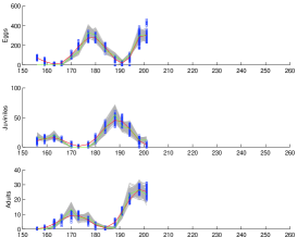
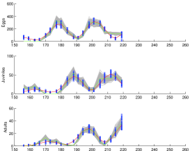
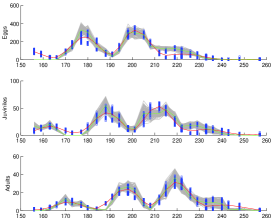
IV
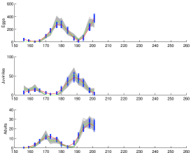
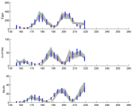
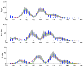
V
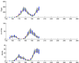
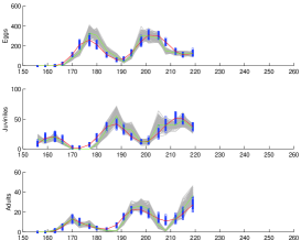
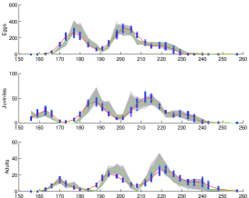
VI

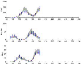
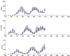
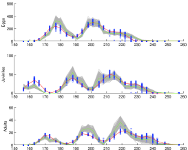
Figure 8: Fits of seasonal models: each panel shows the 100 data sets (grey) for eggs (top), juveniles (middle), and adults (bottom), as well as the values of the fitted models at the data points (blue). Green curve: mean of the 100 data sets; red curve: mean of fitted time series.

Before we offer some consolation to readers who despair at our move from the enlightened monotheism of one growth rate to the heathen polytheism of many growth rates, we are going to use the data shown above to illustrate our thesis. We used six different models to capture the data; see Table 1. The number of parameters varied between 2 for the simple exponential model $N_{0}e^{rt}$ and 12 for the most complex seasonal phenomenological model. The modelling of the data was achieved by standard parameter-fitting methods. The details of the models and the fitting process are not important for this discussion and are therefore omitted. Interested readers may consult the supplementary material available online, which contains some basic information about the models and results. Here it suffices to say that the four seasonal models considered (III-VI in Table 1) are virtually indistinguishable in term of capturing the data (see Fig. 8 of C). By contrast, the two simple non-seasonal growth models (I & II) are rather crude models of the data (see Fig. 7), as expected from the discussion above.

The first four models (I–IV) of the table explicitly contain the growth rate as a parameter. The remaining two are demographic models for which the growth rate is computed from the model parameters according to the Euler–Lotka equation (see eq. (4) in B). The results are tabulated below.

	Time Window
Model	30 days	50 days	70 days	full season
I	0.1160	0.0686	0.0329
II	0.4615	0.4636	0.4789
III		0.0371	0.0552	0.0419
IV		0.1030	0.0620	0.1255
V		0.0311	0.0210	0.0165
VI		0.0498	0.0445	0.0352

Table 2: Growth-rate values derived from various models/time windows.

Looking at Table 2, the conclusion seems inescapable: that one and only growth rate we believed we knew is dead. Using 6 models on 3 time intervals each, results in 18 growth rates! (Although some of the values are fairly close and could be interpreted as representing the same quantity.)

Back to square one?

Maybe we overstated our case when we interpreted the second Sibly-and-Hone quote above as saying that “there are at least two kinds of growth rates". A more adept reading of the quote might be that there are two (or three) ways of determining the growth rate — the implication being that the quantity itself still has a unique “identity". Similarly, we may conclude that what we interpreted as model-dependence of the concept above, may also be interpreted as multiple ways of computing the same ecological quantity, the growth rate. This point of view offers, in fact, an intriguing possibility of “turning the table" on the problem: if we were to assume that the one and only growth rate does exist after all, could we use this to discriminate between the models?

To apply this idea to our field data, we need to mention that the data actually consist of 24 replicates (see Fig. 5 in A); what we showed above were averaged data. To increase the sample size (which we arbitrarily chose to be 100), we used a simple partial averaging technique. For this larger data set (see Fig. 6), we repeated the exercise described above; that is, we fitted the 6 models to each of the 100 data sets and determined the corresponding growth-rate values. Fig. 4 shows the distributions of those values for the various models.

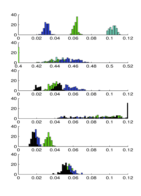
Figure 4: Growth-rate distributions for models I-VI (rows 1-6) using three different time windows for each model. Colour coding of time windows: turquoise - 30 days; green - 50 days; blue - 70 days; black - full season. (Note the different scale in row 2.)

So, which model would you trust? Or, maybe we should say, entrust with determining the “true" growth rate (assuming you believe it exists)?

Obviously, the width/narrowness of the distribution would be a factor in making the decision. Given that the data set was computed from replicates of measurements of the same population, one would expect that the different data sets essentially contain information about the same growth rate (up to some degree of noise), so one would expect the distribution of $r$-values to be fairly narrow as well. This basically eliminates models II and IV, and probably also model III. Perhaps surprisingly, the simplest model (I) has fairly tight distributions, which seems to give it an edge. However, it has a very strong dependence on the time window, over which the fitting is performed. This introduces an unacceptable arbitrariness (how would we tell which time window is the right one?), which leads us to discard this one, too. The best compromise between narrowness of the distribution and independence of the time window seem to be offered by model VI. So we may be inclined to declare this the “winner". It is worth noting that the models that perform best in terms of determining the growth rate $r$ (V & VI) are the ones that do not contain $r$ explicitly.

Of course, there are other factors (likely many) to be considered in selecting models in a particular modelling exercise, such as goodness of fit, complexity, derivability from first principles, purpose etc. (see e.g. [5] and the literature therein). More importantly, the point here is not to actually find the best model for the particular data set shown above. Rather, what we want to point out is that stipulating the existence (or “reality”) of an ecological parameter such as the growth rate can potentially provide an additional robustness criterion. This turns the apparent model dependence of that parameter into a tool for model selection. Ecologists might want try to identify other ecological quantities that could be utilized in a similar manner.

Conclusion

In this paper we offered the reader a choice: abandon the idea of a unique growth rate inherent of a given population and accept that this notion depends on the model used to determine it – or retain the idea of a single growth rate and reject models that are unable to give robust values for it. Is it a matter of mere belief — a mode of mind that many scientists probably feel has no place in scientific inquiry — on which side we come down? Do we even have to decide?

Our final argument is that the two alternatives described above may be used in an iterative manner, much like physicists view the genesis of physical theories. That is, we may take the position that an ecological quantity, such as the growth rate, can only reasonably be assumed to have reality/currency if it can be determined robustly; i.e., if at least one model can be found from which consistent and robust values of that quantity can be derived. If the quantity has gained this kind of credibility, it may be utilized as a criterion for model selection as described above. If one model emerges as particularly suitable in a modelling exercise, it can be checked again for robustness in providing values for the same and/or other credible and established quantities of interest.

As mentioned at the beginning of this story, we feel no urge (and possess no expertise) to enter the philosophical debate surrounding the interrelations of reality (or realism), laws of nature, scientific models etc. and/or the similarities and differences of ecology and the physical sciences. Nor do we make claims about novelty and originality of the ideas described above. For instance, the critical role of models (“nomological machines") and the idea of model robustness have been discussed by Cartwright [3] and Rearinne [18] (following Levins [12]), respectively, as well as others.

All we venture to do here is to advocate a pragmatic view, rooted in the simple (simplistic?) observation that scientific practice often proceeds (well) without explicit reference to abstract foundational thinking. We, the modellers, view the concept of the recursive definition of ecological quantities based on the constructibility and robustness of suitable “nomological machines" as such a pragmatic approach.

Appendix: Supplementary Material

Appendix A Data

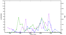
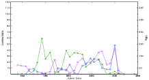
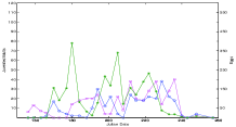
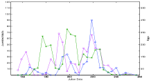
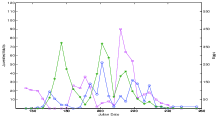
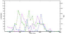
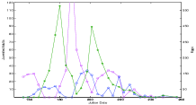
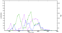
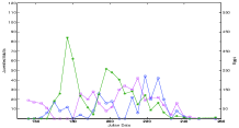
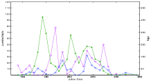
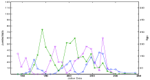
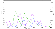
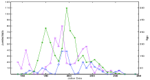
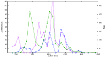
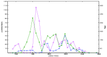
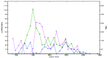
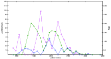
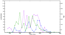
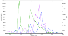
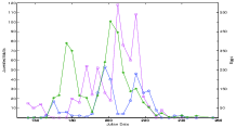
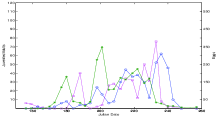
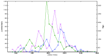
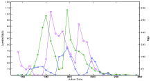
Figure 5: The 24 replicates of the mite data. Fig. 1 shows the life-stage averages of these data. (Colour coding consistent with Fig. 1.)

The growth-rate distributions shown in Fig. 4 and below were computed from an enlarged data set of 100 samples, which were generated by averaging 10 randomly selected data sets of the 24 measured replicates shown in Fig. 5. The resulting 100 times series for each age group are exhibited in Fig. 6 (grey curves).

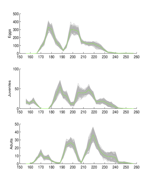
Figure 6: The 100 times series (grey curves) for each life stage: top eggs; middle juveniles; bottom adults. Green curves: means.

Appendix B Models

Simple (non-seasonal) growth models (I & II)

The exponential (I) and logistic (II) models may be parametrized as

$$N(t)=\frac{KN_{0}e^{rt}}{K-N_{0}+N_{0}e^{rt}}$$ (1)

where, formally, the exponential case (I) corresponds to the carrying capacity $K$ becoming arbitrarily large: $K\to\infty$. The other two parameters $N_{0}$ and $r$ have the interpretation of initial population size and growth rate, respectively.

Phenomenological models (III & IV)

Let $X(t)$ be either $E(t)$, $J(t)$, or $A(t)$. Then the seasonal cycle in the data may be modelled by an exponential (III) or logistic (IV) rise (for $t\leq S$), followed by a simple exponential decline ($t>S$):

$$X_{S}(t)=\left\{\begin{array}[]{ll}\frac{KX_{0}e^{rt}}{K-X_{0}+X_{0}e^{rt}},&t\leq S\\ \frac{KX_{0}e^{rS}}{K-X_{0}+X_{0}e^{rS}}e^{-\mu(t-S)},&t>S\end{array}\right.,$$ (2a)

where, as above, the linear case (III) corresponds to the limit $$K\to\infty X_{0},K,r,S,\mu X_{0} K r S \mu$$. The five parameters have the interpretation: initial size of the age group; carrying capacity; growth rate; seasonal parameter: time during the season at which mites stop laying same-season eggs; per-capita death rate.

The purely seasonal curve $X_{S}(t)$ is modulated by generational, non-seasonal, oscillations:

$$X(t)=X_{S}(t)\left[1+I\sin\left(2\pi(t-\phi_{0})/P\right)\right]$$

This adds 3 more parameters: (relative) amplitude $I$, period $P$, and phase shift $\phi_{0}$.

Now letting $X(t)=E(t)$ and assuming that the three age groups only differ by total phase shifts (parameters $\alpha_{0}$ and $\alpha_{1}$) and size (parameters $f$ and $g$), results in the 12-parameter model

$$E(t) = X_{S}(t)\left[1+I\sin\left(2\pi(t-\phi_{0})/P\right)\right]$$ (2b)

$$J(t) = fE(t-\alpha_{0})=fX_{S}(t-\alpha_{0})\left[1+I\sin\left(2\pi(t-\phi_{0}-\alpha_{0})/P\right)\right]\qquad$$ (2c)

$$A(t) = gE(t-\alpha_{1})=gX_{S}(t-\alpha_{1})\left[1+I\sin\left(2\pi(t-\phi_{0}-\alpha_{1})/P\right)\right]\qquad$$ (2d)

Demographic models (V & VI)

The underlying demographic model is the Sharpe-Lotka-McKendrick partial differential equation (PDE) [25]. Under the assumption of piecewise–constant demographic data (fecundity and mortality), delay–differential–equation (DDE) models may rigorously be derived from the full demographic model [8]. These DDE models are reminiscent of ordinary–differential–equation (ODE) compartment models, but they have the advantage of properly accounting for the time individuals spend in the various life stages. Here eggs take $a_{0}$ days to hatch and the emerging juveniles take $\delta$ days to turn into reproducing adults. The model we used reads

$$\dot{E}(t) = e^{a_{0}\mu_{0}}\beta(t)A(t)-\beta(t-a_{0})A(t-a_{0})-\mu_{0}E(t)$$ (3a)

$$\dot{J}(t) = f\beta(t-a_{0})A(t-a_{0})-fe^{-\delta\mu_{1}}\beta(t-a_{1})A(t-a_{1})-\mu_{1}J(t)\qquad$$ (3b)

$$\dot{A}(t) = fe^{-\delta\mu_{1}}\beta(t-a_{1})A(t-a_{1})-\mu_{2}A(t)$$ (3c)

where the $$\dot{X}(t)=\frac{dX}{dt} a_{1}=a_{0}+\delta$$, ,

$$\beta(t)=\beta_{m}e^{-a_{0}\mu_{0}}e^{-\nu M(t)}\left\{\begin{array}[]{cl}1,&t\leq S\\ 0,&t>S\end{array}\right\}\,\textrm{and}\,M(t)=J(t)+A(t).$$ (3d)

The parameters are: $a_{0}$ and $a_{1}=a_{0}+\delta$ – hatching and maturation age; $\mu_{0}$, $\mu_{1}$, and $\mu_{2}$ – per-capita death rate for eggs, juveniles and adults, respectively; $f$ – egg-to-juvenile attrition rate; $\beta_{m}$ – (maximal) fecundity; $\nu$ – nonlinearity coefficient parametrizing the reduction in fecundity due to overcrowding. The linear model (V) arises by setting $\nu=0$.

To obtain unique solutions , the system has to be complemented by initial conditions, which in the case of DDEs, take the form of initial functions, $E_{h}(t),N_{h}(t),A_{h}(t)$ ($0\leq t\leq a_{1}$), called histories. Strictly speaking, prescribing whole functions amounts to prescribing an infinite number of parameters. However, we found that a two-dimensional parameterization of the histories is sufficient in this modelling exercise; we chose the width of the initial age distribution and the total number of beginning-of-season eggs.

The Euler-Lotka equation for this model takes the form

$$\lambda=fe^{-[a_{0}\mu_{0}+\delta\mu_{1}]}\beta_{m}e^{-a_{1}\lambda}-\mu_{2},$$ (4)

i.e. the growth rate (Lotka’s $r$) is the largest real root $r=\lambda$ of (4).

Appendix C Parameter estimation (model fitting)

Model evaluation and fitting was performed in Matlab using standard Matlab routines such as dde23, lsqcurvefit, and nlinfit. The results are visualized in Figures 7 (models I & II) and 8 (models (III–VI).

	Time Window
Model	30 days	50 days	70 days
I
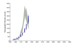
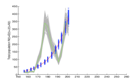
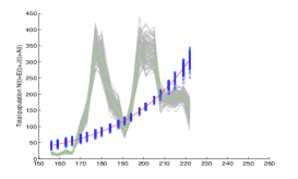
II

Figure 7: Fits of simple (non–seasonal) growth models I & II. Each panel shows the total population $N(t)=E(t)+J(t)+A(t)$ for the 100 data sets (grey) and the values of the fitted models at the data points (blue). Green curve: mean of the 100 data sets; red curve: mean of fitted time series.

Appendix D Growth-rate distributions with error bars

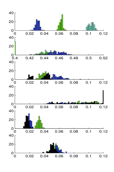
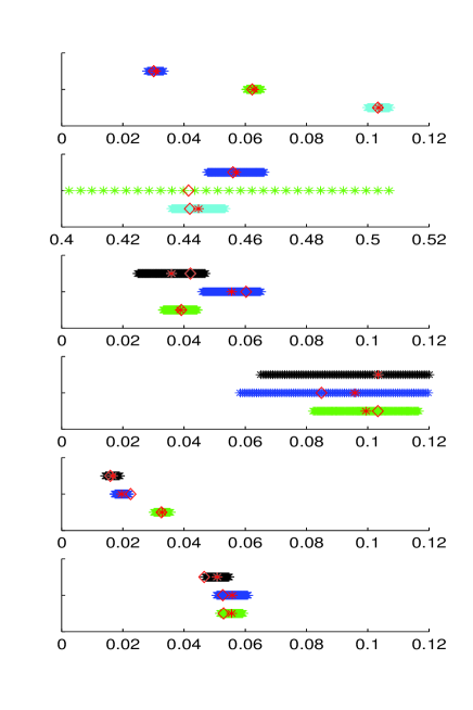
Figure 9: Growth-rate distributions for models I-VI (rows 1-6). Left: Fig. 4. Right: Means (red stars) with error bars (colour coding consistent with left panel); red diamonds: growth-rate values of Table 2 derived from the averaged data displayed in Fig. 1.

These are presented in Fig. 9. For the models in rows I, V and VI we observe that (to a good approximation)

$$\left(\parbox{82.51282pt}{growth rate of {\it averaged} data set}\right)\,=\,\left(\parbox{116.65646pt}{{\it average} of growth rates of individual data sets}\right).$$ (5)

Appendix E Re-weighting age groups 1: ad-hoc method

The weights $w_{1},w_{2},w_{3}$ of the heuristic re-wheighting method described in the main body of the paper were computed as

$$w_{1}=\frac{\int_{0}^{T/2}A(t)dt}{\int_{0}^{T/2}E(t)dt},\quad w_{2}=\frac{\int_{0}^{T/2}A(t)dt}{\int_{0}^{T/2}J(t)dt},\quad w_{3}=1.$$ (6)

where $T$ denotes the length of the season (101 days).

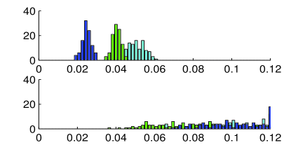
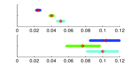
Figure 11: Plot analogous to the first two rows of Fig. 9, but scale in row 2 changed! The dependence on the time window is substantially reduced and identity (5) is satisfied to a high degree.

The growth-rate distributions with errors bars are shown on Fig. 11.

Appendix F Re-weighting age groups 2: reproductive value

	Time Window
Model	30 days	50 days	70 days
I (+V)
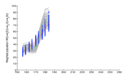
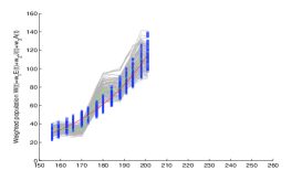
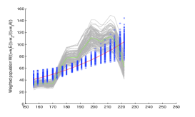
II (+V)
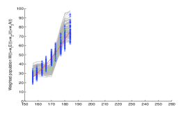
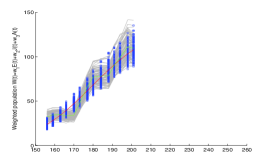
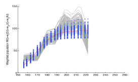
I (+VI)
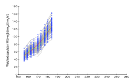
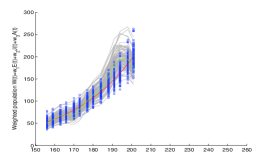
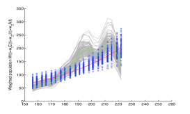
II (+VI)

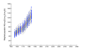
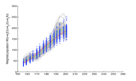
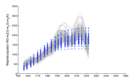
Figure 12: Fits of models I & II to total reproductive value $V(t)$. Rows 1 & 2 and 3 & 4 are analogous to Fig. 10, respectively. Rows 1 & 2: $V(t)$ is computed from the (best-fit) parameter values for the linear demographic model (V). Rows 3 & 4: $V$ is computed from the (best-fit) parameter values for the nonlinear linear demographic model (VI).

As described in the main body of the paper, “naive" aggregate population measures such as the total population may not follow an exponential growth law. Rather, one needs to take an appropriately weighted average (the weight function being given by the (age-dependent) reproductive value $v(a)$) of the various age groups to obtain an exponentially growing quantity (the total reproductive value $V(t)$). Unfortunately, computing $v(a)$ is just as (or even more) involved as determining the growth rate $r$; so the exponential growth law for $V(t)$ does not seem to be of much practical value for finding $r$.

However, this property can be used “after the fact" as another consistency or robustness check for the demographic models. The idea is this: after fitting the models to the data, one can use the (best-fit) model parameters to calculate $V(t)$. In a perfect world, $V(t)$ would be an exponential function $e^{rt}$ with $r$ derived from the Lotka-Euler equation (4). So fitting the simple exponential model (I) to the $V(t)$ time series would just reproduce $r$. Of course, the real world is messier than etherial theory and things are not quite as perfect; see Figures 12 and 13 below, where this procedure was carried out for the model parameters derived from the linear and nonlinear models (V & VI) and the resulting time series $V(t)$ was fitted to the exponential and logistic growth models (I & II).

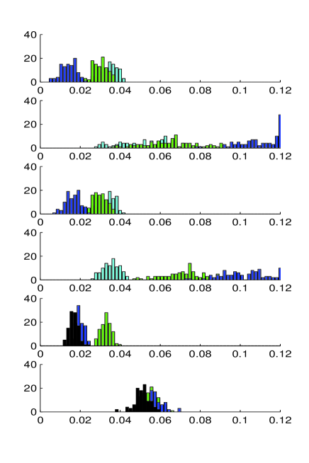
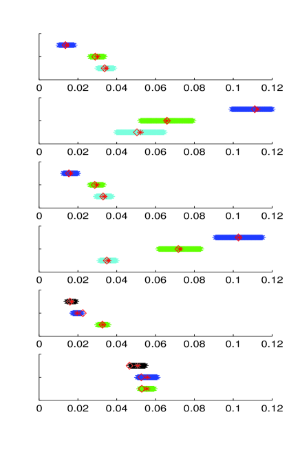
Figure 13: Growth-rate distributions corresponding to Fig. 12 (rows 1-4). Rows 5 and 6 show the distributions derived directly from models V and VI (identical with rows 5 and 6 of Fig. 9); shown for comparison.

References

- [1] Alan A. Berryman. On principles, laws and theory in population ecology. Oikos, 103(3):695–701, 2003.
- [2] Nancy Cartwright. How the laws of physics lie. Clarendon Press, 1983.
- [3] Nancy Cartwright. The dappled world: A study of the boundaries of science. Cambridge University Press, 1999.
- [4] Marvin Chester. A fundamental principle governing populations. Acta Biotheoretica, 60(3):289–302, 2012.
- [5] Matthew R Evans, Volker Grimm, Karin Johst, Tarja Knuuttila, Rogier de Langhe, Catherine M Lessells, Martina Merz, Maureen A O’Malley, Steve H Orzack, Michael Weisberg, et al. Do simple models lead to generality in ecology? to appear in Trends in Ecology & Evolution, 2013.
- [6] Ronald Aylmer Fisher. The actuarial treatment of official birth records. The Eugenics review, 19(2):103, 1927.
- [7] Lev R Ginzburg, Christopher XJ Jensen, and Jeffrey V Yule. Aiming the “unreasonable effectiveness of mathematics" at ecological theory. Ecological Modelling, 207(2):356–362, 2007.
- [8] Joshua Michael Gould. Age-structured population models for species of pest mites. Acadia University, 2007.
- [9] JM Hardman, HJ Herbert, KH Sanford, and D Hamilton. Effect of populations of the european red mite, panonychus ulmi, on the apple variety red delicious in nova scotia. The Canadian Entomologist, 117(10):1257–1265, 1985.
- [10] HJ Herbert. Limits of each stage in populations of the European red mite, Panonychus ulmi. The Canadian Entomologist, 102(01):64–68, 1970.
- [11] HJ Herbert and KH Sanford. The influence of spray programs on the fauna of apple orchards in Nova Scotia: XIX. Apple rust mite, Vasates Schlechtendali, a food source for predators. The Canadian Entomologist, 101(01):62–67, 1969.
- [12] Richard Levins. The strategy of model building in population biology. American Scientist, 54(4):421–431, 1966.
- [13] Dale R Lockwood. When logic fails ecology. The Quarterly Review of Biology, 83(1):57–64, 2008.
- [14] Alfred J Lotka. The stability of the normal age distribution. In Proceedings of the National Academy of Science, volume 8, pages 339–345, 1922.
- [15] DB Marshall and DJ Pree. Effects of miticides on the life stages of the european red mite, panonychus ulmi (koch)(acari: Tetranychidae). The Canadian Entomologist, 123(01):77–87, 1991.
- [16] R.B. O’Hara. The anarchist’s guide to ecological theory. Or, we don’t need no stinkin’ laws. Oikos, 110(2):390–393, 2005.
- [17] Steven Hecht Orzack. The philosophy of modelling or does the philosophy of biology have any use? Philosophical Transactions of the Royal Society B: Biological Sciences, 367(1586):170–180, 2012.
- [18] Jani Raerinne. Robustness and sensitivity of biological models. Philosophical Studies: 1–19, 2012.
- [19] Jani Raerinne. Stability and lawlikeness. Biology & Philosophy: 1–19, 2013.
- [20] R.M. Sibly and J. Hone. Population growth rate and its determinants: an overview. Philosophical Transactions of the Royal Society of London. Series B: Biological Sciences, 357(1425):1153–1170, 2002.
- [21] Fritz Taylor. Convergence to the stable age distribution in populations of insects. American Naturalist, pages 511–530, 1979.
- [22] B. Tenhumberg. Ignoring population structure can lead to erroneous predictions of future population size. Nature Education Knowledge, 1, 2010.
- [23] Peter Turchin. Does population ecology have general laws? Oikos, 94(1):17–26, 2001.
- [24] W.K. Walthall and J.D. Stark. Comparison of two population-level ecotoxicological endpoints: The intrinsic () and instantaneous () rates of increase. Environmental Toxicology and Chemistry, 16(5):1068–1073, 1997.
- [25] G. Webb. Theory of nonlinear age-dependent population dynamics, volume 89. CRC, 1985.