Detrended Cross-Correlation Analysis Consistently Extended to Multifractality

Abstract

We propose a novel algorithm - Multifractal Cross-Correlation Analysis (MFCCA) - that constitutes a consistent extension of the Detrended Cross-Correlation Analysis (DCCA) and is able to properly identify and quantify subtle characteristics of multifractal cross-correlations between two time series. Our motivation for introducing this algorithm is that the already existing methods like MF-DXA have at best serious limitations for most of the signals describing complex natural processes and often indicate multifractal cross-correlations when there are none. The principal component of the present extension is proper incorporation of the sign of fluctuations to their generalized moments. Furthermore, we present a broad analysis of the model fractal stochastic processes as well as of the real-world signals and show that MFCCA is a robust and selective tool at the same time, and therefore allows for a reliable quantification of the cross-correlative structure of analyzed processes. In particular, it allows one to identify the boundaries of the multifractal scaling and to analyze a relation between the generalized Hurst exponent and the multifractal scaling parameter $\lambda_{q}$. This relation provides information about character of potential multifractality in cross-correlations and thus enables a deeper insight into dynamics of the analyzed processes than allowed by any other related method available so far. By using examples of time series from stock market, we show that financial fluctuations typically cross-correlate multifractally only for relatively large fluctuations, whereas small fluctuations remain mutually independent even at maximum of such cross-correlations. Finally, we indicate possible utility of MFCCA to study effects of the time-lagged cross-correlations.

I Introduction

Analysis of time series with nonlinear long-range correlations is often grounded on a study of their multifractal structure halsey86 ; mandelbrot96 ; muzy94 ; kwapien12 ; struzik02 ; oswiecimka05 ; drozdz09 ; mandelbrot89 . Existing algorithms used in such an analysis allow for determining generalized fractal dimensions or Hölder exponents based either on statistical properties of time series kantelhardt02 ; grech13 or on time-frequency information muzy94 ; oswiecimka06 . Because of implementation simplicity and their utility, these algorithms have already been applied to characterize correlation structure of data in various areas of science like physics muzy08 ; subramaniam08 , biology ivanov99 ; makowiec09 ; rosas02 , chemistry stanley88 ; udovichenko02 , geophysics witt13 ; telesca05 , economics ausloos02 ; calvet02 ; turiel05 ; drozdz10 ; oswiecimka08 ; zhou09 ; bogachev09 ; su09 , hydrology koscielny06 , atmospheric physics kantelhardt06 , quantitative linguistics ausloos12 ; grabska12 , music jafari07 ; oswiecimka11 , and human communications perello08 . As an important step towards quantifying complexity, in recent years algorithms designed for investigation of fractal cross-correlations were proposed podobnik08 ; podobnik09 followed by the new statistical cross-correlation tests zebende11 ; podobnik11 . These developments are based on the Detrended Cross-Correlation Analysis (DCCA) which constitutes a straightforward generalization of the fractal auto-correlation (DFA) kantelhardt01 on the case of fractally cross-correlated signals. In that case, the cross-correlation scaling exponent $\lambda$ can be obtained. However, literature still lacks comprehensive interpretation of this quantity.

Subsequently, the multifractal extension (MF-DXA) of the DCCA method was proposed zhou08 . Other closely related methods to deal with multifractal cross-correlations have also been introduced kristoufek11 . However, these extensions naturally involve computation of arbitrary powers of cross-covariances and this leads to serious limitations since such cross-covariances may, in general, become negative. In such a case the net result, expressed in terms of the usual fluctuation functions, thus becomes complex-valued which does not allow to determine the scaling exponents by conventional means. A simplistic resolution, so far available in the literature, to this difficulty is based on taking modulus jiang11 ; he11 ; li12 ; wang12 of the cross-covariance function in order to get rid of its negative signs. In most realistic cases, as our analysis below shows, this however seriously distorts or even spuriously amplifies the multifractal cross-correlation measures. Our motivation therefore is to elaborate an algorithm that we call Multifractal Cross-Correlation Analysis (MFCCA), such that for any two signals it allows to compute their arbitrary-order covariance function and at the same time it properly takes care of the relative signs in the signals.

The proposed method allows us to calculate the spectrum of the exponents $\lambda_{q}$, which characterize multifractal properties of the cross-covariance. However, unlike the method proposed ealier, in our procedure, the scaling properties of the $q$th order cross-covariance function are estimated with respect to the original sign of the cross-covariance. This procedure makes the method both more sensitive to cross-correlation structure and free from limitations of other algorithms. It also turns out that the proposed method is a more natural generalization of the monofractal DCCA than is MF-DXA. The robustness of our algorithm makes it applicable to different data types in various fields of science.

II Description of the MFCCA algorithm

Multifractal Cross-Correlation Analysis consists of several steps which are described in detail below. As it was mentioned above, MFCCA has been developed based on the DCCA procedure podobnik08 , therefore the initial steps are the same.

Consider two time series $x_{i}$, $y_{i}$ where $i=1,2...N$. At first, the signal profile has to be calculated for each of them:

$$X\left(j\right)=\sum_{i=1}^{j}[x_{i}-\langle x\rangle],\quad Y\left(j\right)=\sum_{i=1}^{j}[y_{i}-\langle y\rangle].$$ (1)

Here, $\langle\rangle$ denotes averaging over entire time series. Then, both signal profiles are divided into $M_{s}=N/s$ disjoint segments $\nu$ of length $s$. For each box $\nu$, the assumed trend is estimated by fitting a polynomial of order $m$ ($P^{(m)}_{X,\nu}$ for $X$ and $P^{(m)}_{Y,\nu}$ for $Y$). Based on our own experience oswiecimka06 , as optimal we use a polynomial of order $m=2$ throughout this paper but the proposed procedure is not restricted to this particular order and can be used for much larger one when needed (as, for instance, in signals involving a highly periodic component horvatic11 ; ludescher11 ). Next, the trend is subtracted from the data and the detrended cross-covariance within each box is calculated:

$$F_{xy}^{2}(\nu,s)=\frac{1}{s}\Sigma_{k=1}^{s}\{(X((\nu-1)s+k)-P^{(m)}_{X,\nu}(k))\times\\ \times(Y((\nu-1)s+k)-P^{(m)}_{Y,\nu}(k))\}$$ (2)

In contrast to the detrended variance calculated in the MFDFA procedure kantelhardt02 , in the present case, $F_{xy}^{2}(\nu,s)$ can take both positive and negative values (for an example see Sec. III.3 Fig.12). Therefore, gradual investigation of scaling properties from small to large fluctuations through their covariances of increasing order should take into account also sign of $F_{xy}^{2}(\nu,s)$. Accordingly, the most natural form of the $q$th order covariance function is postulated by the following equation:

$$F_{xy}^{q}(s)=\frac{1}{M_{s}}\Sigma_{\nu=1}^{M_{s}}{\rm sign}(F_{xy}^{2}(\nu,s))|F_{xy}^{2}(\nu,s)|^{q/2},$$ (3)

where ${\rm sign}(F_{xy}^{2}(\nu,s))$ denotes the sign of $F_{xy}^{2}(\nu,s)$. The parameter $q$ can take any real number except zero. However, for $q=0$, the logarithmic version of Eq. (3) can be employed kantelhardt02 :

$$F_{xy}^{0}(s)=\frac{1}{M_{s}}\Sigma_{\nu=1}^{M_{s}}{\rm sign}(F_{xy}^{2}(\nu,s))\ln|F_{xy}^{2}(\nu,s)|.$$ (4)

As we can see in Eq. (3), for negative values of $q$, small values of the covariance function $F_{xy}^{2}(\nu,s)$ are amplified, while for large $q>0$, its large values dominate. Moreover, the formula for calculating $F_{xy}^{q}(s)$ respects the genuine signs of the amplified (or supressed) fluctuations of the detrended cross-covariance function (Eq. (2)) and, at the same time, it allows to avoid complex numbers associated with the arbitrary powers of negative fluctuations. The above described steps of MFCCA should be repeated for different scales $s$. If the so-obtained function $F_{xy}^{q}(s)$ does not develop scaling, by for instance fluctuating around zero, there is no fractal cross-correlation between the time series under study for the considered value of $q$. Multifractal cross-correlation is expected to manifest itself in the power-law dependence of $F_{xy}^{q}(s)$ (if the $q$th order covariance function is negative for every $s$, we may take $F_{xy}^{q}(s)\longrightarrow-F_{xy}^{q}(s)$ podobnik08 ) and the following relation is fulfilled:

$$F_{xy}^{q}(s)^{1/q}=F_{xy}(q,s)\sim s^{\lambda_{q}}$$ (5)

(or $\exp(F_{xy}^{0}(s))=F_{xy}(0,s)\sim s^{\lambda_{0}}$ for $q=0$), where $\lambda_{q}$ is an exponent that quantitatively characterizes fractal properties of the cross-covariance. For the monofractal cross-correlation, the exponents $\lambda_{q}$ are independent of $q$ and equal to $\lambda$ as obtained from the DCCA method. In the case of multifractal cross-correlation, however, $\lambda_{q}$ varies with $q$, with $\lambda$ retrieved for $q=2$. The minimum and maximum scales ($s_{min}$ and $s_{max}$, respectively) depend on the length $N$ of the time series under study. In practice, it is reasonable to take $s_{max}<N/5$.

III Analysis of examplary models and stock market data

In order to verify the usefulness of MFCCA algorithm, we test it by using both artificially generated cross-correlated time series and real-world signals. In order to avoid divergent moments due to fat tails in the distribution of fluctuations, we restrict $q$ to $\langle-4,4\rangle$ with a step $0.2$ throughout this paper. In the case of computer-generated signals, results for each process are averaged over its 20 independent realizations.

III.1 ARFIMA processes

Figure 1: (Color online) (Left) Family of the $q$th-order cross-covariance functions $F_{xy}(q,s)$ calculated for ARFIMA processes for three different combinations of the parameters $H_{1}$ and $H_{2}$. The lowest and the highest line in each panel refers to $q=-4$ and $q=4$, respectively. (Right) Multifractal cross-correlation scaling exponents $\lambda_{q}$ (black circles) and the average generalized Hurst exponents $h_{xy}(q)$ (red squares). Error bars indicate standard deviation calculated from 20 independent realizations of the corresponding processes.

We start our study from an analysis of the well-known ARFIMA processes hosking81 , which are examples of monofractal, long-range correlated signals. In Ref. podobnik08 , such processes were used to show usefulness of the DCCA algorithm. Our goal is to show the cross-correlation structure of the above-mentioned processes more completely. To generate a pair ($x_{i},y_{i}$) of the cross-correlated ARFIMA processes, we use the following equations:

$$x_{i}=\Sigma_{j=1}^{\infty}a_{j}(d_{x})x_{i-j}+\epsilon_{i}\,$$ (6)

$$y_{i}=\Sigma_{j=1}^{\infty}a_{j}(d_{y})y_{i-j}+\epsilon_{i}$$ (7)

where $d_{x}$ and $d_{y}$ are parameters characterizing linear long-range autocorrelations of the times series. These quantities can be related to the Hurst exponents kantelhardt01 by the relation $H=1/2+d_{x(y)}$, ($-1/2<d_{x(y)}<1/2$). Positively correlated (persistent) time series are characterized by $H>0.5$, whereas negative autocorrelation (antipersistent signal) is characterized by $H<0.5$; H=0.5 means no linear autocorrelation. The quantity $a_{j}(d_{x(y)})$ is called weight and is defined by $a_{j}(d_{x(y)})=\Gamma(j-d_{x(y)})/[\Gamma(-d_{x(y)})\Gamma(1+j)]$, where $\Gamma()$ stands for Gamma function. $\epsilon_{i}$ is an i.i.d. Gaussian random variable. The processes $x_{i}$ and $y_{i}$ are cross-correlated, because the same noise component $\epsilon_{i}$ is used in both Eq.(6) and Eq.(7). We generate three pairs of cross-correlated signals: ($H_{1}$=0.5, $H_{2}$=0.6), ($H_{1}$=0.5, $H_{2}$=0.7), and ($H_{1}$=0.5, $H_{2}$=0.9), where $H_{1}$ and $H_{2}$ characterize long-range autocorrelation of the first and the second time series, respectively. In order to obtain statistically significant results, we generate time series of lengh $N=100,000$ points each.

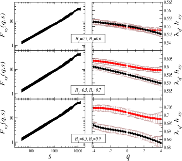
In the left panels of Fig. 1, we present the calculated $F_{xy}(q,s)$ for all the signal pairs. Each line corresponds to a different value of $q$. As it can be seen, in all the cases, $F_{xy}(q,s)$ is a power function of scale $s$. This indicates the fractal nature of the cross-correlations. Moreover, for all types of signals, the functions $F_{xy}(q,s)$ are almost parallel to each other implying largely homogeneous character of the corresponding cross-correlations. Indeed, as shown in the right panels of the Fig. 1, the difference between the extreme values of $\lambda_{q}$ expressed by $\Delta\lambda_{q}=\max(\lambda_{q})-\min(\lambda_{q})$ is approximately 0.005, 0.007, and 0.011 for the top, middle, and the bottom panel, respectively. These narrow ranges of $\lambda_{q}$ indicate that the ARFIMA processes reveal correlations that are monofractal regardless of the types of linear autocorrelation of signals.

In literature, the estimated fractal cross-correlations are often related to the fractal properties of the individual signals themselves podobnik08 ; siqueira10 ; shadkhoo09 . Therefore, in Fig. 1, we also show the average of the generalized Hurst exponents  kantelhardt02 :

$$h_{xy}(q)=(h_{x}(q)+h_{y}(q))/2,$$ (8)

where $h_{x}(q)$ and $h_{y}(q)$ refer to fractal properies of individual time series, respectively and, for $q=2$, they correspond to the Hurst exponent $H$. It is worth noticing that relation between $\lambda_{q}$ and $h_{xy}(q)$ depends on temporal organization of the signals as determined by their Hurst exponents. For two signals whose Hurst exponents $H$ are alike, their multifractal cross-correlation characteristics described by $\lambda_{q}$ and $h_{xy}(q)$ are almost identical, while the divergence between $\lambda_{q}$ and $h_{xy}(q)$ becames more sizeble for time series with more significant differences in autocorrelation (different Hurst exponent $H$).

This result means that, in the case of the ARFIMA processes, the relation $\lambda\approx(h_{x}(2)+h_{y}(2))/2$ introduced in Ref. podobnik08 applies only to a situation when differences between $h_{x}$ and $h_{y}$ are negligible.

III.2 Markov-switching multifractal model

As an example of multfractal process, we consider the Markov-switching multifractal model (MSM) liu07 . MSM is an iterative model, which is able to replicate hierarchical, multiplicative structure of real data and, thus, insures multifractal properties of the generated time series. Because of its properties, MSM is commonly used in finance, where multifractality of price fluctuations is one of the main stylized facts liu08 ; kwapien05 . Equally well this model can be used to simulate many other multifractal time series representing natural phenomena as it is able to generate the volatility clustering responsible for the underlying nonlinear temporal correlations drozdz09 . Below, we present the main stages of the model’s construction.

Figure 2: (Color online) (Left) Family of the $q$th-order cross-covariance functions $F_{xy}(q,s)$ calculated for two pairs of the MSM time series corresponding to $m_{0}^{(1)}=1.2$, $m_{0}^{(2)}=1.35$ (top) and $m_{0}^{(1)}=1.2$, $m_{0}^{(2)}=1.6$ (bottom). The lowest and the highest line on each panel refers to $q=-4$ and $q=4$, respectively. (Right) Multifractal cross-correlation scaling exponents $\lambda_{q}$ (black circles) and the average generalized Hurst exponents $h_{xy}(q)$ (red squares). Insets present the differences between $\lambda_{q}$ and $h_{xy}$.

Figure 3: (Color online) (Inset) Average $\lambda_{2}=\lambda$ and average $h_{xy}(2)$ as a function of $\Delta m_{12}=m_{0}^{(2)}-m_{0}^{(1)}$. Black circles and red squares correspond to the $\lambda$ and $h_{xy}(2)$, respectively. Error bars indicate standard deviation calculated from 20 independent realizations of the corresponding process. (Main) Difference of the average $\lambda$ and the average $h_{xy}(2)$ as a function of $\Delta m_{12}$.

In MSM, evolution of an observable $r_{t}$ in time $t$ is modeled by the formula liu08 :

$$r_{t}=\sigma_{t}\cdot u_{t},$$ (9)

where $u_{t}$ stands for a Gaussian random variable and $\sigma_{t}$ (multifractal process) stands for the instantaneous volatility component. The volatility $\sigma_{t}$ is a product of $k$ multipliers $M_{1}(t),M_{2}(t),...,M_{k}(t)$ such that

$$\sigma^{2}_{t}=\sigma^{2}\prod_{i=1}^{k}M_{i}(t),$$ (10)

where $\sigma^{2}$ is a constant factor. A common version of the model assumes that the multipliers $M_{i}(t)$ are drawn from the binomial or from the log-normal distribution. Here, we use the binomial one with $M_{i}(t)\sim\{m_{0},2-m_{0}\}$, $1\leq m_{0}<2$. Any change of a multiplier in the hierarchical structure of volatility is determined by the transition probabilities liu07 :

$$\gamma_{i}=1-(1-\gamma_{k})^{b^{i-k}},\quad i=1,2...k.$$ (11)

Thus, a multiplier $M_{i}(t)$ is renewed with probability $\gamma_{i}$ and remains unchanged with probability $1-\gamma_{i}$. The parameter $\gamma_{k}$ is taken from the range $(0,1)$, and $b>1$. We put $\gamma_{k}=0.5$ and $b=2$, which leads to the relation:

$$\gamma_{i}=1-(0.5)^{2^{i-k}},\quad i=1,2...k.$$ (12)

Thus, for the initial stages of the cascade, a renewal of the multipliers $M_{i}(t)$ occurs with relatively small probability, while the largest $\gamma_{i}=0.5$ appears for $i=k$.

III.2.1 Unsigned version of the MSM model

For the purpose of this analysis, we generate a set of multifractal time series ($\sigma_{t}$) of length $131,072$ points each. However, in all realizations of the model, we conserve the hierarchical structure of the multipliers, since the renewals of $M_{i}(t)$ appear for the same $i$ and $t$ in each generated series. This procedure insures cross-correlations between series with different $m_{0}$.

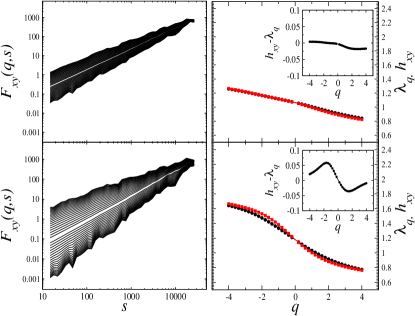
In Fig. 2, we present sample results of MFCCA obtained for two pairs of MSM series with the parameters $m_{0}^{(1)}=1.2$ and $m_{0}^{(2)}=1.35$ (top panels) and $m_{0}^{(1)}=1.2$ and $m_{0}^{(2)}=1.6$ (bottom panels). The $q$th-order covariance functions $F_{xy}(q,s)$ (left hand side of this Figure) display a clear multifractal scaling within the whole range $(-4,4)$ of the $q$ values. The resulting $\lambda_{q}$ is a decreasing function of $q$, which is a hallmark of multifractality. Moreover, the rate of decrease of $\lambda_{q}$ depends on the values of mutlipliers. For the first pair of signals (with $m_{0}^{(2)}=1.35$), the exponents $\lambda_{q}$ are contained in the range (0.81,1.25), while for the second pair (with $m_{0}^{(2)}=1.6$), $0.75\leq\lambda_{q}\leq 1.7$. In the same Fig. 2, we also show the average of the generalized Hurst exponents calculated for each time series independently (red squares).

Interestingly, for the signals with a relatively small difference $\Delta m_{12}=m_{0}^{(2)}-m_{0}^{(1)}$ - in other words, for similar multifractals - $\lambda_{q}$ approximately equals the average of $h_{x}(q)$ and $h_{y}(q)$. A tiny difference between $h_{xy}(q)$ and $\lambda_{q}$ is here visible only for $q>0$. This effect is depicted more quantitatively in the insets of Fig. 2, where $h_{xy}(q)-\lambda_{q}$ is presented as a function of $q$. The maximum deviation from zero can be seen for $q=2.2$, reaching a value of $0.02$. For the second pair of signals, the difference $h_{xy}(q)-\lambda_{q}$ is more pronounced and concerns both negative and positive $q$’s. In this case, the largest difference of $h_{xy}(q)$ and $\lambda_{q}$ is for $q=-2$ and equals 0.07.

III.2.2 Relation between $\lambda_{q}$ and $h_{xy}$

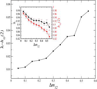
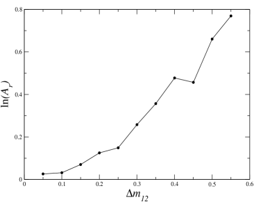
To have some insight into the relation between $\lambda_{q}$ and $h_{xy}(q)$, we perform a systematic MFCCA study for the set of time series pairs, such that one of them is generated with $m_{0}^{(1)}=1.2$ and the other one with $m_{0}^{(2)}$ from the range $\langle 1.25,1.9\rangle$ (the step is 0.05). However, the multifractal characteristics were possible to estimate only for $\Delta m_{12}<0.6$. In the case of $\Delta m_{12}>0.6$, $F_{xy}^{q}$ takes both positive and negative values and Eq.(5) is not satisfied. At first, we focus on the relationship between $\lambda_{2}=\lambda$ and the average Hurst exponent $h_{xy}(2)$. In the inset of Fig. 3, we present these quantities as a function of $\Delta m_{12}$. It is clearly visible that both these quantities are monotonically decreasing and they take approximately the same values for small $\Delta m_{12}$. However, for $\Delta m_{12}>0.25$, $\lambda(\Delta m_{12})$ decreases slower than the Hurst index (thus $\lambda>H$) and the statistics diverge. To highlight this result, we calculate also the difference between these two quantities which is shown in Fig.3. As one can see, $\lambda-h_{xy}(2)$ is an increasing function of $\Delta m_{12}$. This result indicates that the difference between $\lambda$ and the average Hurst exponent becomes larger for time series whose multifractal characteristics depart more from each other, while the opposite is observed when these characteristics are alike, which at the same time results in stronger cross-correlations.

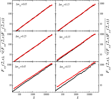
To better understand this effect, we analyze a covariance function $F_{xy}(2,s)\sim s^{\lambda}$ and an expression based on fluctuation functions kantelhardt02 : $\sqrt{F_{xx}(2,s)F_{yy}(2,s)}\sim s^{\frac{h_{x}(2)+h_{y}(2)}{2}}=s^{h_{xy}(2)}$. In Fig. 4, we show these functions calculated for different values of $\Delta m_{12}$. It is easy to notice that the presented functions are almost identical to each other for small $\Delta m_{12}$. However, the larger $\Delta m_{12}$ is, the more visible is a departure between the analyzed statistics. In all cases, the values of $F_{xy}(2,s)$ are at most equal to $\sqrt{F_{xx}(2,s)F_{yy}(2,s)}$ and estimated $\lambda$ is larger than $h_{xy}(2)$. These numerical results are in accord with the following relation:

$$F_{xy}(2,s)\leq\sqrt{F_{xx}(2,s)F_{yy}(2,s)},$$ (13)

which straightforwardly results from the definitions of these quantities considered in terms of the scalar products of vectors formed from the underlying time series he11 . In order to more clearly see the relationship between $\lambda$ and $h_{xy}(2)$, we can reformulate Eq. (13) in the case when the relations $F_{xy}(2,s)=a_{xy}s^{\lambda}$, $F_{xx}(2,s)=a_{x}s^{h_{x}(2)}$, and $F_{yy}(2,s)=a_{y}s^{h_{y}(2)}$ apply, to obtain:

$$a_{xy}s^{\lambda}\leq(a_{x}a_{y})^{1/2}s^{\frac{h_{x}(2)+h_{y}(2)}{2}}.$$ (14)

This leads to:

$$\lambda\leq\log_{s}(\frac{(a_{x}a_{y})^{1/2}}{a_{xy}})+\frac{h_{x}(2)+h_{y}(2)}{2}.$$ (15)

For two identical time series, the equality in Eq. (13) holds leading to obvious $\lambda=\frac{h_{x}(2)+h_{y}(2)}{2}$. In general, however,

$$A_{r}=\frac{(a_{x}a_{y})^{1/2}}{a_{xy}}\neq 1,$$ (16)

and thus a difference between $\lambda$ and $h_{xy}(2)$ in either direction is allowed or even forced, depending on a sign of $\log_{s}(A_{r})$. For negative values of this quantity, $\lambda$ has to be smaller than $h_{xy}(2)$, while for positive values it can become larger. An example demonstrating the rate of changes of $\ln(A_{r})$ as a function of $\Delta m_{12}$ for $q=2$ is shown in Fig. 5. In this case, $\ln(A_{r})$ is positive and quickly increases with $\Delta m_{12}$, thus with the degree of dissimilarity between the two series. The related dependencies are even more involved and appear to strongly vary with the parameter $q$ as it is more systematically shown in Fig. 6. The $\ln(A_{r})$ is seen to be positive for $q>0$ with an increasing value at maximum with increasing $\Delta m_{12}$, and a larger amplitude of changes with increasing $q$. Similar, but reversed in sign and with an even larger amplitude of changes, is the situation for $q<0$. These results nicely coincide - and thus point to their origin - with those presented in Fig. 2, where $\lambda_{q}$ is larger than $h_{xy}(q)$ for positive values of $q$ and smaller for negative ones. Even the maxima of these differences occur for those values of $q$, where they are seen in Fig. 6 and they are larger on the negative side of $q$. Of course, they are also larger for larger $\Delta m_{12}$.

Figure 4: (Color online) Comparision of covariance function $F_{xy}(2,s)$ (black circles) with its equivalent $\sqrt{F_{xx}(2,s)F_{yy}(2,s)}$ (red squares) derived from the variance functions of individual MSM time series. The slope of this functions refers to $\lambda_{2}$ and $h_{xy}(2)$, respectively.

Figure 5: Plot of $\ln(A_{r})$ calculated for $q=2$ as a function of similarity parameter $\Delta m_{12}$ of the MSM time series.

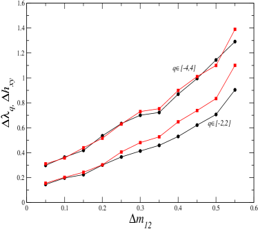
The difference between $\lambda_{q}$ and $h_{xy}(q)$ has its reflection - also consistent with the findings presented in Figs. 2 and 6 - in another popular multifractal measure, namely in the range of scaling exponents. In Fig. 7, we display $\Delta\lambda_{q}$ as a function of $\Delta m_{12}$ for the two ranges of $q$: $-2\leq q\leq 2$ and $-4\leq q\leq 4$. For comparison, in the same Figure, we show $\Delta h_{xy}=\max(h_{xy})-\min(h_{xy})$ calculated for the same ranges of $q$. The $\Delta h_{xy}(q)$ and $\Delta\lambda_{q}$ are seen to be monotonically increasing functions of $\Delta m_{12}$ in all the cases. However, for $-4\leq q\leq 4$ these characteristics are almost the same, while for $-2\leq q\leq 2$ the difference between $\Delta h_{xy}$ and $\Delta\lambda_{q}$ systematically increases with $\Delta m_{12}$. This suggests that for relatively large values of $|q|$ (magnifying the largest and the smallest fluctuations of instantaneous volatility components) the fractal character of the considered processes is similar, which may reflect the effect of preserving the same hierarchical structure of multipliers for all generated multifractals, where only relative changes of volatility are possible. The above results thus indicate that the difference between $h_{xy}(q)$ and $\lambda_{q}$ is to be considered an important ingredient of measure of the fractal cross-correlation between two time series.

Figure 6: Plot of $\ln(A_{r})$ as a function of $q$. Each line corresponds to different degree of similarity $\Delta m_{12}$ of the MSM time series.

Figure 7: (Color online) $\Delta\lambda_{q}$ (black circles) and $\Delta h_{xy}$ (red squares) as functions of multiplier difference $\Delta m_{12}=m_{0}^{(2)}-m_{0}^{(1)}$ calculated for two ranges of the parameter $q$.

III.2.3 Performance comparison of MFCCA and MF-DXA

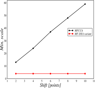
In the next stage of our study of the MSM generated $\sigma_{t}$ time series, we analyze output of MFCCA if one time series of a pair is gradually being shifted in time with respect to the other one. Then the correlations, especially their fractal character, should undergo an obvious weakening. This test is aimed at further verifying performance of the algorithm. As an input, we use a time series with $m_{0}=1.2$ and the same one, but shifted by a certain number of points. We notice that the larger is the relative shift between the time series, the shorter is the scaling range of $F_{xy}$. However, in all cases, the estimated $\lambda$ is equal to the generalized Hurst exponent calculated for a single series. This shortening of the range of scaling is not symmetric from both sides of the scale range, but gradually arrives entirely from the small scale side. The shift dependence of the lower bound of the scaling regime that can be used to determine $\lambda_{q}$ is shown in Fig. 8. As expected, lifting of this lower bound is seen to be almost linear. In the same Figure, we also present the result of an analogous analysis, but performed by means of the common variant of the MF-DXA procedure that, in order to resolve the sign problem, makes use of the absolute values of the fluctuation functions jiang11 ; he11 ; li12 ; wang12 . In this case, the procedure is seen not to be sensitive to this type of surrogate and, thus, evidently generates spurious cross-correlations.

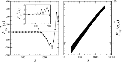
In order to elaborate more in detail on this last issue, we generate an example of a pair of the MSM time series with $m_{0}=1.2$ drawn independently, i.e., with no taking care about preserving the hierarchical structure of the multipliers. Even though individually both such series are multifractal with the same multifractality characteristics, there is no reason to expect them to be multifractally cross-correlated. Indeed, in the present case the corresponding $q$th order covariance functions determined through the Eq. (3) do not scale and for small and moderate scales they even assume the negative values by fluctuating around zero. An example of $F^{2}_{xy}(s)$ demonstrating this behavior is shown in the left panel of Fig. 9. In fact, this dependence closely resembles the DCCA result (Fig. 1b in ref. podobnik08 ) obtained in an analogous situation of the two uncorrelated series. This correspondence thus provides an additional argument that it is MFCCA proposed here that constitutes a natural and correct multifractal generalization of DCCA. Application of a previously postulated zhou08 extension of DCCA in the present example would lead to complex-valued $q$th-order covariances. As already mentioned in Introduction, a commonly adopted resolution to this difficulty is based on taking modulus of the cross-covariance before computing its $q$th order. The result of such a procedure applied to our example of two independently generated MSM time series with $m_{0}=1.2$ is shown in the right panel of Fig. 9 and it clearly indicates a convincing multifractal scaling. This, of course, is however a false signal as these series are not expected to be multifractally correlated.

Figure 8: (Color online) Lower bound of the scaling regime that can be used in the calculation of $\lambda_{q}$ as a function of the shift between two independent realizations of the MSM time series with $m_{0}=1.2$. Black circles and red squares refer to calculations performed by means of MFCCA and a commonly adopted ’modulus’ variant of the MF-DXA procedure, respectively.

Figure 9: (Left) 2nd-order covariance function $F_{xy}^{2}(s)$ obtained by means of MFCCA for two independently generated MSM time series with $m_{0}=1.2$. (Inset) The same function for a shorter range of scales $s$. (Right) A family of the $F_{xy}(q,s)$ functions calculated by means of the ’modulus’ variant of MF-DXA. The lowest and the highest line refers to $q=-4$ and $q=4$, respectively.

III.2.4 Signed version of the MSM model

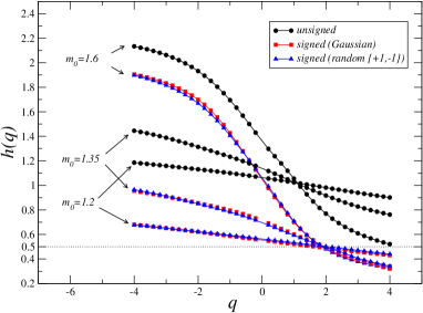
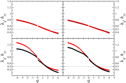
The time series of $\sigma_{t}$ considered above represent unsigned fluctuations (volatility in financial terms) and therefore their individual Hurst exponents are significantly larger than 0.5. By incorporating the Gaussian random variable $u_{t}$ drawn from $N(0,1)$ through the Eq. (9), one obtains the signed time series $r_{t}$ with the Hurst exponents close to 0.5 (as for the financial returns, for instance). Very similar effect one obtains when multiplying the original unsigned fluctuations simply by randomly drawn either $+1$ or $-1$. The influence of such procedures on the generalized Hurst exponents $h(q)$ is shown in Fig. 10 for the same pairs of the MSM time series as before, i.e., with $m_{0}=1.2,m_{0}=1.35$ and $m_{0}=1.2,m_{0}=1.6$. Circles indicate $h(q)$ for the original unsigned series while squares and triangles indicate the series signed by the Gaussian random variable and by the pure random sign, respectively. Introducing sign clearly shifts the lines down relative to the unsigned case, such that the usual Hurst exponent $H=h(2)$ assumes value of $0.5$ for all the signed series. The $q$-dependence of $h(q)$, naturally stronger for larger $m_{0}$, remains however essentially preserved after introducing the sign, which reflects the fact that such an operation influences primarily the linear temporal correlations in the series leaving the nonlinear ones, related to the volatility clustering drozdz09 , preserved. As far as multifractal cross-correlations between such series are concerned, more care is needed. Drawing the term $u_{t}$ in Eq. (9) independently for the two series destroys their original (unsigned) cross-correlations and the corresponding $q$th-order covariances calculated through the Eq. (3) develop similar fluctuations as those in the left panel of Fig. 9. One most straightforward way to preserve multifractal cross-correlations is to use the same $u_{t}$ for the two series under consideration. Examples of the so-prepared pairs of series, for the same combination of the parameters $m_{0}$ as before for the unsigned series, i.e., $m_{0}=1.2$ versus $m_{0}=1.35$ and $m_{0}=1.2$ versus $m_{0}=1.6$, are analyzed in Fig. 11 in terms of $\lambda_{q}$ and $h_{xy}(q)$. For the first of these pairs, irrespective of the sign adding variant, the multifractal cross-correlations are seen to remain essentially on the same level of strength as those for the corresponding unsigned signals shown in the upper panel of Fig 2. The departures between $\lambda_{q}$ and $h_{xy}(q)$ for the other pair ($m_{0}=1.2$ and $m_{0}=1.6$) of the signed series can be seen to be somewhat larger relative to their unsigned counterparts, which signals slight weakening of their multifractal cross-correlations. This in fact is consistent with the generalized Hurst exponents $h(q)$ seen in Fig. 10. When sign is applied to the series, the distance between the corresponding $h(q)$ routes increases, especially on the negative $q$ side, as compared to the unsigned case.

Figure 10: (Color online) Generalized Hurst exponent $h(q)$ calculated for individual MSM time series. The circles refer to the original unsigned series while squares and triangles refer to the series signed by the Gaussian random variable and by pure random sign, respectively.

Figure 11: (Color online) $q$th-order fluctuation function scaling exponent $\lambda_{q}$ (black circles) and the average generalized Hurst exponent $h_{xy}(q)$ (red squares) calculated for two pairs of signed MSM time series corresponding to $m_{0}^{(1)}=1.2$, $m_{0}^{(2)}=1.35$ (top) and $m_{0}^{(1)}=1.2$, $m_{0}^{(2)}=1.6$ (bottom). (Left) MSM time series signed by a Gaussian random variable. (Right) MSM time series signed by a pure random sign.

III.3 Examples of stock market data

The financial fluctuations can be considered a physical process which constitutes one of the most complex generalizations of the conventional Brownian motion carrying at the same time convincing traces of nontrivial fractality mandelbrot97 ; bogachev07 ; ludescher11b . They therefore offer a very demanding territory to test the related concepts and algorithms. For this reason, as final examples of utility of the MFCCA method, we present an analysis of empirical data coming from the German stock exchange. Furthermore, since multifractal analysis of financial data is one of the most informative methods of investigating such complex systems oswiecimka05 ; drozdz10 ; zhou09 ; kwapien05 ; lopez03 , we believe that MFCCA will be very useful in this field as well. We consider logarithmic price increments $g(i)$ and linear time increments $\Delta t(i)$ representing dynamics of a sample German stocks - E.ON (ticker: EOA) and Deutsche Bank (ticker: DBK) (from the same database as used before oswiecimka05 ) being part of the DAX30 index. These quantities are obtained according to the formulas:

$$g(i)=\ln(p(i+1))-\ln(p(i)),\ \$$ (17)

$$\Delta t(i)=t(i+1)-t(i),$$ (18)

where $p(i),i=1,...,N$ is a time series of price quotes taken in discrete transaction time $t(i)$. As it has been shown previously oswiecimka05 , both $g(i)$ and $\Delta t(i)$ are processes with self-similar structure and could be analyzed by the multifractal methods. Quantifying the character of cross-correlations just between these two characteristics of the financial dynamics is also of particular importance for forecasting volatility within models such as the Multifractal Model of Asset Returns mandelbrot96 ; mandelbrot97 ; lux03 ; oswiecimka06b ; eisler04 . Our analysis is performed on time series comprising the period between Nov. 28, 1997 and Dec. 31, 1999. The time series consists of $T=294,862$ and $T=497,513$ points for EOA and DBK, respectively. Therefore, the time series are long enough to bring statistically significant results.

Figure 12: Top and middle: detrended variance functions $F_{xx}^{2}(\nu,500)$ and $F_{yy}^{2}(\nu,500)$ calculated for time series of price increments and waiting times of E.ON stock (ticker: EOA), respectively. Bottom: detrended cross-covariance function $F_{xy}^{2}(\nu,500)$ calculated for the same data. Calculations were carried out for segments of length of 500 points.

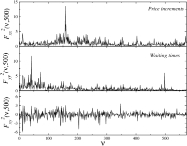
In Fig. 12, we show one of the first steps of our algorithm, i.e., the detrended cross-covariance function $F^{2}_{xy}(\nu,500)$ (for the scale $s=500$) as a function of the box number $\nu$ (Eq. (2)). For comparison, in the same Fig. 12, we depicted the detrended variance function $F_{xx}^{2}(\nu,500)$ and $F_{yy}^{2}(\nu,500)$ (obtained from MFDFA) calculated for individual time series of price increments and waiting times, respectively. It is easy to notice that the detrended variance calculated for individual time series takes only positive values, whereas the detrended cross-covariance function $F_{xy}^{2}(\nu,s)$ takes both negative and positive values. This constitutes the already-mentioned principal problem in straightforward calculation of the $q$th-order cross-covariance function $F_{xy}(q,s)$ for odd $q$s that results in complex values of this function (see Eq. (5)). It is worth stressing that this difficulty does not affect the fractal analysis of individual time series (MFDFA), because then the detrended variance function $F_{xx}^{2}(\nu,s)$ may only be positive. It follows that proper handling of the sign of $F_{xy}^{2}(\nu,s)$ is of crucial importance for a consistent extension of DCCA to treat the multifractally correlated signals. At present, a solution of this problem is offered only by the MFCCA algorithm proposed in Sec. II.

In order to characterize the cross-correlations in the present case, the function $F_{xy}(q,s)$ is calculated. As far as the multifractal scaling is concerned, the situation is significantly more subtle than in the previous model cases. It turns out that the scaling property of $F_{xy}(q,s)$ applies only selectively. First of all, for the negative $q$s, $F_{xy}^{q}(s)$ fluctuates around zero and Eq. (5) is not satisfied. For positive values of $q$, the function $F_{xy}^{q}(s)$ assumes positive values but clear scaling of $F_{xy}(q,s)$ begins with $q=1$ upwards. For $q<1$, these functions develop increasing fluctuations when $q$ moves towards zero. This effect is especially strong for DBK. Furthermore, the lower limit of scales where $F_{xy}(q,s)$ develops the convincing power-law behavior varies and it takes place at the higher values of $s$ for DBK than for EOA, which signals a weaker form of multifractal cross-correlation in the former case. The corresponding characteristics are shown in the upper panels of Fig. 13 with the scaling bounds both in $q$ and in $s$ indicated by the dashed lines.

Figure 13: (Color online) (Top) Family of the $F_{xy}(q,s)$ functions calculated for time series of price increments and waiting times of E.ON (EOA) and Deutsche Bank (DBK). The lowest and the highest line on each panel refers to $q=0.2$ and $q=4$, respectively. The dashed lines indicate scaling bounds both in $q$ and $s$. (Bottom) Multifractal cross-correlation exponent $\lambda_{q}$ (black circles) and the average generalized Hurst exponents $h_{xy}(q)$ (red squares) for the same data as above. The exponents $\lambda_{q}$ are estimated only for $1\leq q\leq 4$.

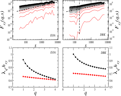
The calculated $\lambda_{q}$ and $h_{xy}(q)$ are shown in the bottom panels of Fig. 13. It is clearly visible that, for EOA, both functions converge to each other for large values of $q$, while $\lambda_{q}$ is significantly larger than $h_{xy}(q)$ for smaller values of $q$. These results imply that the scaling properties of $F_{xy}(q,s)$ strongly depend on the considered time span and they cannot be fully quantified by a unique exponent $\lambda$. Moreover, based on our results for the MSM model, we can infer that the analyzed processes are ruled by the similar fractal dynamics only in periods with relatively large $F_{xy}^{2}(\nu,s)$ (associated with large $q$). For smaller $q$’s, the difference between $\lambda_{q}$ and $h_{xy}(q)$ is more evident, which suggests that dynamics of these processes is significantly different, but still cross-correlative. It is worth to mention that large values of $F_{xy}^{2}(\nu,s)$ can be a consequence of cross-correlation both in the signs and the amplitudes of the signals. However, the waiting times are unsigned and the price increments are signed, but the sign is uncorrelated. This means that, in our case, the amplitude of $F_{xy}^{2}(\nu,s)$ is only a result of the cross-correlation of the observed amplitude. The strong cross-correlation of volatility (modulus of time series) is confirmed by Fig.14, where the cross-correlation function for the waiting times and absolute values of the price increments is depicted. Therefore, we conclude that large fluctuations are much more strongly cross-correlated than the smaller ones. Complexity of the multifractal cross-correlation is expressed by the range of $\lambda_{q}$ that is approximately $0.32$ in this case.

Figure 14: (Color online) Cross-correlation function $C_{xy}(\tau)=|x_{i+\tau}||y_{i}|$ corresponding to modulus of price increments and transaction times of EOA (black squares) and DBK (red circles). Inset: the same function but calculated for randomly shuffled data.

As may be anticipated already from the structure of $F_{xy}(q,s)$ for DBK, the behavior of $\lambda_{q}$ is slightly different and the difference between $h_{xy}(q)$ and $\lambda_{q}$ is substantial both for small and for large values of $q$ (Fig. 13, right panel). Also $\Delta\lambda_{q}$ for DBK is smaller than in the case of EOA and takes a value of $0.22$. This suggest that although structure of the cross-correlation between the inter-transaction times and the price increments for DBK is multifractal, its heterogeneity is poorer than in the case of EOA. Moreover, similarity between the fractal dynamics of large fluctuations is not so evident than in the former case. These results are also confirmed by Fig. 14, where a difference between the strength of volatility cross-correlations for both considered stocks is easily visible.

The results presented here indicate that the multifractal cross-correlation characterizes only relatively large fluctuations of the signals under study. Smaller fluctuations that are filtered out by $q<1$, from the perspective of multifractal cross-correlation, may be considered mutually independent.

In connection with the present example we also wish to mention - but without showing the results explicitly in order not to confuse the reader - that taking absolute values of the fluctuation functions to get rid of the sign problem (as recently often done in literature he11 ; li12 ; wang12 ), in the present financial data case, would result in a convincing but apparent multifractal scaling for all values of $q$, similar to one that we have already seen for the MSM model in Fig. 9. Also, the so determined $\lambda_{q}$ equals $h_{xy}(q)$ as in the MSM model. This way one, however, does not extract genuine correlations, but only measures the averaged multifractal properties of individual time series.

Another type of correlations that are of theoretical as well as of practical interest are the correlations among stock returns kwapien12 ; mantegna00 . These are typically quantified in terms of the Pearson correlation coefficients or, more generally, in terms of the correlation matrix. This way of quantifying correlations is, however, restricted to their linear component only. The present formalism of studying the multifractal cross-correlations allows one to reveal some of their potential nonlinear components. As an example, we therefore use the same two stocks as above (EOA and DBK) and, in addition, Commerzbank (CBK) from the same, German stock exchange over the same period, and perform a similar analysis as above for two pairs of time series (CBK-DBK and DBK-EON) representing the corresponding 1 min returns. Over the period considered, this yields 267,241 data points. The results in the same representation as before are presented in Fig. 15.

Figure 15: (Color online) (Top) Family of the $q$th-order cross-covariance functions $F_{xy}(q,s)$ calculated for 1 min returns of two pairs of stocks corresponding to Commerzbank (CBK) and Deutsche Bank (DBK), and Deutsche Bank and E.ON (EOA). The lowest and the highest line on each panel refers to $q=0.2$ and $q=4$, respectively. The dashed lines indicate scaling bounds both in $q$ and $s$. (Bottom) Multifractal cross-correlation exponent $\lambda_{q}$ (black circles) and the average generalized Hurst exponents $h_{xy}(q)$ (red squares) for the same data. Calculation of $\lambda_{q}$ was restricted to $0.6\leq q\leq 4$.

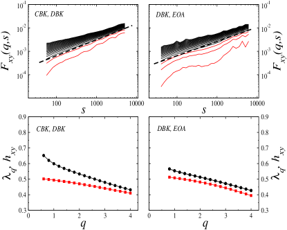
For $q<0$, the $F_{xy}(q,s)$ are not drawn since the corresponding $F_{xy}^{q}(s)$ functions fluctuate around zero. As we go to the positive $q$ values, however, they start developing a convincing scaling already for $q=0.6$ (as indicated by the dashed lines) for both pairs and for all the scales considered. This scaling is clearly multifractal and the resulting $\lambda_{q}$ and $h_{xy}(q)$, shown in the lower panels of Fig. 15, are somewhat closer to each other than the ones previously considered for correlations between the price increments and the inter-transaction times. Slight differences in relation between the present two pairs of time series are also visible, however. For DBK-EON, the departures between $\lambda_{q}$ and $h_{xy}(q)$ are largely independent on $q$ in the region where scaling applies, while for CBK-DBK it starts from larger values for the smallest $q$-values (0.6), but it converges to even smaller values with an increasing $q$. This can be interpreted as an indication that multifractal character of cross-correlations resembles more each other for CBK and DBK on the level of large fluctuations and weakens for the smaller ones, while, within the pair DBK-EON, they are of similar strength in the comparable range of fluctuation size. Of course, in both cases this kind of cross-correlations disappears on the level of small fluctuations that are filtered out by the negative values of $q$, and this seems quite a natural effect in the financial context.

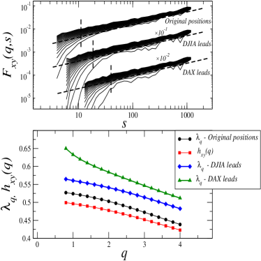
As a final example indicating possible applications of the MFCCA method introduced in this paper, we study the cross-correlations between the two world leading stock market indices, the Dow Jones Industrial Average (DJIA) and the Deutscher Aktienindex (DAX), based on their daily returns. The period considered for both these indices begins on January 12, 1990 and ends on October 12, 2013. This results in time series of length of 5881 data points. Due to different time zones which the two indices are traded in and in order to test potential applicability of the present algorithm in detecting possible time-lags or asymmetry effects in correlations, we study three possible variants of positioning the time series relative to each other. The first variant is most natural, i.e., data points in the two time series meet each other at the same date they are recorded. The other two variants are such that the time series are shifted by one day relative to each other, either DAX is advanced by one day or DJIA is. The corresponding $F_{xy}(q,s)$ functions are displayed in the upper panel of Fig. 16. Unlike the high-frequency recordings discussed above, the significantly shorter time series in the present case restrict us to cover a smaller scale range. Nevertheless, evident multifractal scaling can still be identified in this case as indicated by the dashed lines in Fig. 16, provided the range of $q$ is restricted as well. Similarly to the situation with the high frequency cross-correlations within the German stocks, here $F_{xy}^{q}(s)$ also fluctuates around zero for negative $q$s, and therefore the corresponding functions $F_{xy}(q,s)$ are not shown. Interestingly, the lower bound in $s$ where scaling starts visibly lifts up as we move from the same date, through the situation described as ’DJIA leads’, and becomes the shortest in the situation ’DAX leads’. Accordingly, the departures between $h_{xy}(q)$, which, of course, remains invariant with respect to such relative shifts of the time series, and $\lambda_{q}$ increase as we go through the above three relative locations of DJIA versus DAX (lower panel of Fig. 16). The strongest DJIA-DAX multifractal cross-correlation is detected when the series are originally arranged relative to each other. Their relative 1-day shifts reveal an effect of asymmetry, however. The situation ’DJIA leads’ preserves significantly more of such cross-correlations than the opposite ”DAX leads’ one. This result can be interpreted as an indication that the DJIA close has more influence on the DAX close next day than the DAX close has on the DJIA close next day. In fact, as verified additionaly, splitting the time series considered here into two halves shows that this effect is more evident in 1990’s than more recently. Such an asymmetry in information transfer between these two stock markets is understandable in economic terms, and in fact it is also consistent with the previous study drozdz01 based on the correlation matrix formalism. Finally, we wish to mention that more distant relative shifts of the two present time series quickly deteriorate the multifractal cross-correlation, while at the same time the modulus-based MF-DXA approach leaves them unchanged.

Figure 16: (Color online) (Top) Three families of the $q$th-order cross-covariance functions $F_{xy}(q,s)$ calculated for different synchronization levels of time series representing daily returns of two market indices, DJIA and DAX: (1) the synchronous (original) index positions, (2) DAX retarded by one day with respect to DJIA (DJIA leads), and (3) vice versa (DAX leads). For clarity, the functions $F_{xy}(q,s)$ for ’DJIA leads’ and ’DAX leads’ are vertically shifted. The lowest and the highest line for each considered case refers to $q=0.2$ and $q=4$, respectively. The dashed lines indicate scaling bounds both in $q$ and $s$. (Bottom) Multifractal cross-correlation exponent $\lambda_{q}$ and the average generalized Hurst exponents $h_{xy}(q)$ calculated for the corresponding time series ($0.8\leq q\leq 4$).

IV Summary and conclusions

We proposed an algorithm, which we called Multifractal Cross-Correlation Analysis, that allows for quantitative description of multiscale cross-correlations between two time series and that is free of limitations the other existing algorithms, like MF-DXA, suffer from. The key point that distinguishes MFCCA from other related methods is construction of the $q$th-order cross-covariance function $F_{xy}^{q}(s)$ in Eq.(3), which preserves the sign of the cross-covariance fluctuation function $F_{xy}^{2}(\nu,s)$ after its modulus has been raised to a power of $q/2$. This step has two immediate consequences: (1) it eliminates the risk of appearance of complex values that might lead to problems with their correct interpretation, and (2) it prohibits losing information that is stored in the negative cross-covariance. It follows that, as we showed in Sec. III.2 regarding known model data, the results obtained with MFCCA are more logical and better coincide with intuition than do the parallel results of MF-DXA. This was true both for the signed and the unsigned, volatility-like processes. On this ground we concluded that MFCCA provides us with the most complete information about fractal cross-correlations possible as compared to the other related methods existing so far. Having realized this, we applied MFCCA to sample real-world data from the stock markets. We found that both the cross-stock correlations and the lagged inter-market correlations of returns, as well as the correlations between price movements and the corresponding transaction time intervals are clearly multifractal. Moreover, we showed that carriers of these cross-correlations are predominantly the large fluctuations in both signals, while the smaller fluctuations contribute rather little. This outcome may suggest that an important ingredient of financial complexity, which manifests itself here as multifractality, might be temporal relations between large events.

Apart from the introduction of MFCCA, we also focused our attention on the relation between the $q$th-order scaling exponent $\lambda_{q}$ and the averaged generalized Hurst exponents $h_{xy}(q)$. Both these measures are equally important if one intends to comprehend fractal structure of the data under study. This is because their spectra analyzed in parallel for each signal separately contain information about similarity of their fractal structure. For example, based on model data, we found that the larger is the difference between $\lambda_{q}$ and $h_{xy}(q)$, the more different are the considered (multi)fractals. We thus strongly recommend investigation of both these quantities in parallel.

We believe that our approach presented here will allow for a wider application of multifractal cross-correlation analysis to empirical data in different areas of science.

V Acknowledgements

The calculations were done at the Academic Computer Centre CYFRONET AGH, Kraków, Poland (Zeus Supercomputer) using Matlab environment.

References

- (1) T.C. Halsey, M.H. Jensen, L.P. Kadanoff, I. Procaccia, and B.I. Shraiman, Phys. Rev. A 33, 1141 (1986).
- (2) B.B. Mandelbrot, A.J. Fisher, and L.E. Calvet, Cowles Fundation Discussion Paper No. 1164 (1996).
- (3) J.-F. Muzy, E. Bacry, and A. Arneodo, Int. J. Bifur. Chaos 4, 245 (1994).
- (4) J. Kwapień, and S. Drożdż, Phys. Rep 515, 115 (2012).
- (5) Z.R. Struzik, and A.P.J.M. Siebes, Physica A 309, 388 (2002).
- (6) P. Oświȩcimka, J. Kwapień, and S. Drożdż, Physica A 347, 626 (2005).
- (7) S. Drożdż, J. Kwapień, P. Oświȩcimka, and R. Rak, EPL 88, 60003, (2009).
- (8) B. B. Mandelbrot, Pure Appl. Geophys. 131, 5 (1989).
- (9) J.W. Kantelhardt, S. A. Zschiegner, E. Koscielny-Bunde, S. Havlin, A. Bunde, and H.E. Stanley, Physica A 316, 87 (2002).
- (10) D. Grech and Z. Mazur, Phys. Rev. E 87, 052809 (2013).
- (11) P. Oświȩcimka, J. Kwapień, and S. Drożdż, Phys. Rev. E 74, 016103 (2006).
- (12) J.F. Muzy, E. Bacry, R. Baile, and P. Poggi, EPL 82, 60007 (2008).
- (13) A.R. Subramaniam, I.A. Gruzberg, and A.W.W. Ludwig, Phys. Rev. B 78, 245105 (2008).
- (14) P.Ch. Ivanov, L. A. N. Amaral, A. L. Goldberger, S. Havlin, M. G. Rosenblum, Z. R. Struzik, and H. E. Stanley, Nature 399, 461 (1999).
- (15) D. Makowiec, A. Dudkowska, R. Gała̧ska, and A. Rynkiewicz, Physica A 388, 3486 (2009).
- (16) A. Rosas, E. Nogueira Jr., and J.F. Fontanari, Phys. Rev. E 66, 061906 (2002).
- (17) H.E. Stanley and P. Meakin, Nature 335, 405 (1988).
- (18) V.V. Udovichenko and P.E. Strizhak, Theor. Exp. Chem. 38, 259 (2002).
- (19) A. Witt and B.D. Malamud, Surv. Geophys. 34, 541 (2013).
- (20) L. Telesca, V. Lapenna, and M. Macchiato, New J. Phys. 7, 214 (2005).
- (21) M. Ausloos and K. Ivanova, Comp. Phys. Comm. 147, 582 (2002).
- (22) L. Calvet and A. Fisher, Rev. Econ. Stat. 84, 381 (2002).
- (23) A. Turiel and C.J. Perez-Vicente, Physica A 355, 475 (2005).
- (24) S. Drożdż, J. Kwapień, P. Oświȩcimka, and R. Rak, New J. Phys. 12 105003 (2010).
- (25) P. Oświȩcimka, J. Kwapień, S. Drożdż, A.Z. Górski, and R. Rak, Acta Phys. Pol. A 114, 547 (2008).
- (26) W.-X Zhou, EPL 88, 28004 (2009).
- (27) M.I. Bogachev and A. Bunde, Phys. Rev. E 80, 026131 (2009).
- (28) Z.-Y. Su, Y.-T.Wang and H.-Y. Huang, J. Korean Phys. Soc. 54, 1395 (2009).
- (29) E. Koscielny-Bunde, J.W. Kantelhardt, P. Braund, A. Bunde and S. Havlin, J. Hydrology 322, 120 (2006).
- (30) J.W. Kantelhardt, E. Koscielny-Bunde, D. Rybski, P. Braun, A. Bunde and S. Havlin, J. Geophys. Res. (Atmosph.) 111, D01106 (2006).
- (31) M. Ausloos, Phys. Rev. E 86, 031108 (2012).
- (32) I. Grabska-Gradzińska, A. Kulig, J. Kwapień, P. Oświȩcimka and S. Drożdż, AWERProcedia Information Technology & Computer Science 03, 1700 (2013).
- (33) G.R. Jafari, P. Pedram, and L. Hedayatifar, J. Stat. Mech., P04012 (2007).
- (34) P. Oświȩcimka, J. Kwapień, I. Celińska, S. Drożdż, and R. Rak, arXiv:1106.2902, 2011.
- (35) J. Perello, J. Masoliver, A. Kasprzak, and R. Kutner, Phys. Rev. E 78, 036108 (2008).
- (36) B. Podobnik and H.E. Stanley, Phys. Rev. Lett. 100, 084102 (2008).
- (37) B. Podobnik, D. Horvatic, A. M. Petersen, and H. E. Stanley, Proc. Natl. Acad. Sci. USA 106, 22079 (2009).
- (38) G.F. Zebende, Physica A 390, 614 (2011).
- (39) B. Podobnik, Z.-Q. Jiang, W.X. Zhou, and H.E. Stanley, Phys. Rev. E 84, 066118 (2011).
- (40) J.W. Kantelhardt, E. Koscielny-Bunde, H.H.A Rego, S. Havlin, and A. Bunde, Physica A 295, 441 (2001).
- (41) W.-X Zhou, Phys. Rev. E 77, 066211 (2008).
- (42) L. Kristoufek, EPL 95, 68001 (2011).
- (43) Z.-Q. Jiang and W.-X. Zhou, Phys. Rev. E 84, 016106 (2011).
- (44) L.-Y. He and S.-P. Chen, Physica A 390, 297 (2011).
- (45) Z. Li and X. Lu, Physica A 391, 3930 (2012).
- (46) G.-J. Wang and C. Xie, Acta Phys. Pol. B, 43 2021 (2012).
- (47) D. Horvatic, H.E. Stanley and B. Podobnik, EPL 94, 18007 (2011).
- (48) J. Ludescher, M.I. Bogachev, J.W. Kantelhardt, A.Y. Schumann, A. Bunde, Physica A 390, 2480 (2011).
- (49) J. Hosking, Biometrika 68, 165 (1981).
- (50) E. L. Siqueira Jr., T Stošić, L. Bejan, and B. Stošić, Physica A 389, 2739 (2010).
- (51) S. Shadkhoo and G.R. Jafari, Eur. Phys. J. B 72, 679 (2009).
- (52) R. Liu, T. Di Matteo, and T. Lux, Physica A 383, 35 (2007).
- (53) R. Liu, T. Di Matteo, and T. Lux, Kiel Working Paper No. 1427 (2008).
- (54) J. Kwapień, P. Oświȩcimka, and S. Drożdż, Physica A 350, 466 (2005).
- (55) B.B. Mandelbrot, Fractal and Scaling in Finance: Discontinuity, Concentration, Risk (Springer, New York, 1997).
- (56) M. I. Bogachev, J. F. Eichner, and A. Bunde, Phys. Rev. Lett. 99, 240601 (2007).
- (57) J. Ludescher, C. Tsallis, and A. Bunde, EPL 95, 68002 (2011).
- (58) J.L. López, and J.G. Contreras, Phys. Rev E 87, 022918 (2013).
- (59) T. Lux, University of Kiel, Working Paper No. 2003-13 (2013).
- (60) P. Oświȩcimka, J. Kwapień, S. Drożdż, A.Z. Górski and R. Rak, Acta Phys. Pol. B 37, 3083 (2006).
- (61) Z. Eisler and J. Kertesz, Physica A 343, 603 (2004).
- (62) R.N. Mantegna and H.E. Stanley, An Introduction to Econophysics (Cambridge University Press, Cambridge, 2000).
- (63) S. Drożdż, F. Grümmer, F. Ruf and J. Speth, Physica A 294, 226 (2001).