Light-Cone Distribution Amplitudes
for Heavy-Quark Hadrons

Abstract

We construct parametrizations of light-cone distribution amplitudes (LCDAs) for $B$-mesons and $\Lambda_{b}$-baryons that obey various theoretical constraints, and which are simple to use in factorization theorems relevant for phenomenological applications in heavy-flavour physics. In particular, we find the eigenfunctions of the Lange-Neubert renormalization kernel, which allow for a systematic implementation of renormalization-group evolution effects for both $B$-meson and $\Lambda_{b}$-baryon decays. We also present a new strategy to construct LCDA models from momentum-space projectors, which can be used to implement Wandzura-Wilczek–like relations, and which allow for a comparison with theoretical approaches that go beyond the collinear limit for the light-quark momenta in energetic heavy-hadron decays.

1 Motivation

Light-cone distribution amplitudes (LCDAs) play a key role in the factorization of short- and long-distance dynamics entering exclusive transition amplitudes in Quantum Chromodynamics (QCD). Defined as hadronic matrix elements of composite QCD operators with fields separated along the light-cone, they represent genuine non-perturbative quantities, whose renormalization-scale dependence follows from the anomalous dimension of the defining operators which can be computed in perturbation theory. While early analyses focused on light hadrons (pions, kaons, nucleons, etc. Efremov:1979qk ; Lepage:1979zb ; Duncan:1979hi ; Chernyak:1983ej ), with the running $b$-physics program at “B-Factories” or high-luminosity hadron colliders, the interest in exclusive decay channels of $B$-mesons and $\Lambda_{b}$-baryons revealed the importance of LCDAs for hadrons containing a heavy quark. For instance, the former provide the dominant hadronic input for the theoretical description of radiative leptonic $B$-decays Korchemsky:1999qb ; DescotesGenon:2002mw ; Lunghi:2002ju ; Bosch:2003fc ; Beneke:2011nf ; Braun:2012kp , they enter the QCD-factorization approach for non-leptonic and semi-leptonic $B$-decays Beneke:1999br ; Beneke:2000wa ; Bosch:2001gv ; Ali:2001ez ; Beneke:2001at ; Kagan:2001zk , and they naturally appear in the context of soft-collinear effective theory (SCET) Bauer:2000yr ; Beneke:2002ph . They can also be used in correlation functions that form the basis of light-cone sum rules for heavy-to-light transition form factors DeFazio:2005dx ; Khodjamirian:2005ea , and they appear as limiting cases in the $k_{T}$-factorization approach for heavy-meson Keum:2000wi ; Lu:2000em or heavy-baryon He:2006ud decays.

Theoretical properties of LCDAs have been classified for heavy mesons (see e.g. Grozin:1996pq ; Beneke:2000wa ; Kawamura:2001jm ) and heavy baryons (see e.g. Ball:2008fw ; Feldmann:2011xf ; Ali:2012pn ). The renormalization-group (RG) evolution of the LCDAs has been derived in the heavy-quark limit, where the $b$-quark fields are treated in heavy-quark effective theory (HQET), for both, mesons Lange:2003ff ; Braun:2003wx ; Lange:2004yh ; Lee:2005gza ; Bell:2008er ; DescotesGenon:2009hk ; Knodlseder:2011gc and baryons Ball:2008fw . Available model parametrizations are typically inspired by sum-rule analyses, for instance Braun:2003wx for $B$-mesons or Ball:2008fw for $\Lambda_{b}$-baryons. Certain inverse moments of the $B$-meson LCDA can also be constrained from experimental data, most notably from the radiative leptonic decay $B\to\gamma\ell\nu$ (see Beneke:2011nf ; Braun:2012kp for recent analyses).

In this article, our aim is to improve the theoretical modelling of LCDAs for $B$-mesons and $\Lambda_{b}$-baryons in two aspects: First, we introduce a new representation for LCDAs in terms of a convolution of Bessel functions and a spectral function, which behaves in a dual way compared to the original LCDAs. This representation diagonalizes the Lange-Neubert (LN) evolution kernel, and therefore greatly simplifies the analytic solution of the RG equation. Our formalism also provides a systematic method to include the Efremov-Radyushkin–Brodsky-Lepage (ERBL) kernel, which arises from gluon exchange among the light spectator quarks in the $\Lambda_{b}$-baryon. — Second, we develop a general procedure for an efficient modelling of LCDAs, starting from momentum-space projectors, which satisfy the equations of motion for the partonic Fock-state components. In this approach, the LCDAs follow as simple integrals over a set of (fewer) on-shell wave functions, which allows for a comparison between LCDAs used in the collinear factorization approach and transverse-momentum-dependent wave-functions employed in the $k_{T}$-factorization approach. For $B$-mesons, our formalism reproduces the so-called Wandzura-Wilczek (WW) relations established in Beneke:2000wa , and for $\Lambda_{b}$-baryons, we derive analogous relations between the various 3-particle LCDAs.

Our paper is organized as follows. In the first part, we focus on $B$-meson LCDAs for which we first recollect the main definitions and results, before we introduce our new representation in terms of dual spectral functions and give a detailed discussion on the RG properties. As a sample application of our formalism, we briefly reconsider the RG-improved factorization formula for the radiative leptonic $B\to\gamma\ell\nu$ decay. We proceed with the definition of on-shell momentum-space wave functions, and show how to construct the LCDAs and the corresponding momentum-space projectors to be used in applications of (collinear) QCD factorization. We also discuss how to incorporate corrections to the WW relations from 3-particle Fock states, and discuss two simple wave function models in detail. — In the second part we present an analogous analysis for baryon LCDAs. Here, we show that the momentum-space construction – together with some simplifying assumptions – leads to an enormous reduction of independent hadronic functions. The RG equations for the baryon LCDAs are more complicated than for the meson LCDAs, because the LN kernel and the ERBL kernel depend differently on the two light-quark momenta. Nevertheless, we show that the RG equations can be solved systematically in the dual space in an expansion in Gegenbauer polynomials. This also establishes the general properties of leading-twist baryon LCDAs in the asymptotic limit.

Our results are shortly summarized in Section 4. In the appendix we generalize our results for the $B$-meson momentum-space projectors to an arbitrary frame, where the heavy quark has a transverse velocity component. We also provide some details about the ERBL evolution of the baryon LCDAs, and collect some general integral relations for Bessel functions.

2 $B$–Mesons

2.1 Light-Cone Distribution Amplitudes

We first recapitulate the properties of $B$-meson LCDAs in the heavy-quark limit, see e.g. Grozin:1996pq and references therein.

2.1.1 Light-Cone Projector for 2-Particle Fock State

The 2-particle LCDAs of the $B$-meson in HQET (which differ from the QCD definition, see Pilipp:2007sb ; Li:2012md ) can be obtained from the coordinate-space matrix elements

$$\langle 0|\bar{q}^{\beta}(z)\,[z,0]\,h_{v}^{\alpha}(0)|\bar{B}(v)\rangle$$ (1)

$$=-\frac{i\tilde{f}_{B}m_{B}}{4}\left[\frac{1+\not{v}}{2}\left\{2\,\tilde{\Phi}_{B}^{+}(t,z^{2})+\frac{\tilde{\Phi}_{B}^{-}(t,z^{2})-\tilde{\Phi}_{B}^{+}(t,z^{2})}{t}\,\not{z}\right\}\gamma_{5}\right]^{\alpha\beta}\,,$$ (2)

in the limit of light-like separation $z^{2}\to 0$. Here $t=v\cdot z$, and $[z,0]$ denotes a gauge-link represented by a straight Wilson line along $z^{\mu}$. The heavy $b$-quark field in HQET is denoted as $h_{v}$ for a $B$-meson that moves with velocity $v^{\mu}$. The decay constant $\tilde{f}_{B}$ in the heavy-quark limit includes the non-trivial scale dependence from the non-vanishing anomalous dimension of the local heavy-to-light current in HQET.

The terms in curly brackets can be expanded around $z^{2}=0$, using the power-counting induced by the convolution with generic hard-scattering kernels in factorization theorems (see the discussion in Beneke:2000wa ). Introducing light-like vectors $n_{\pm}^{\mu}$ with $(n_{-}\!\cdot\!n_{+})=2$ and $v^{\mu}=\frac{n_{-}^{\mu}+n_{+}^{\mu}}{2}$, and taking $(n_{-}z)\ll z_{\perp}\ll(n_{+}z)$, we obtain

$$2\,\tilde{\Phi}_{B}^{+}(t,z^{2})+\frac{\tilde{\Phi}_{B}^{-}(t,z^{2})-\tilde{\Phi}_{B}^{+}(t,z^{2})}{t}\,\not{z}$$ (3)

$$\stackrel{{\scriptstyle\not{v}\to 1}}{{\longrightarrow}}\quad \tilde{\phi}_{B}^{+}(\tau)\,\not{n}_{+}+\tilde{\phi}_{B}^{-}(\tau)\,\not{n}_{-}+\frac{\tilde{\phi}_{B}^{-}(\tau)-\tilde{\phi}_{B}^{+}(\tau)}{\tau}\,\not{z}_{\perp}+{\cal O}(z_{\perp}^{2},n_{-}z)\,,$$ (4)

where $t\to\tau=\frac{n_{+}z}{2}$ can be interpreted as the Fourier-conjugated variable to the momentum component $\omega=(n_{-}k)$ associated with the light anti-quark field. Defining the LCDAs in momentum space from the Fourier transform,

$$\phi_{B}^{\pm}(\omega) \equiv\int\frac{d\tau}{2\pi}\,e^{i\omega\tau}\,\tilde{\phi}_{B}^{\pm}(\tau)\,,$$ (5)

the light-cone expansion in (4) corresponds to the momentum-space projector Beneke:2000wa

$${\cal M}_{B}(v,\omega) =-\frac{i\tilde{f}_{B}m_{B}}{4}\left[\frac{1+\not{v}}{2}\bigg{\{}\phi_{B}^{+}(\omega)\,\not{n}_{+}+\phi_{B}^{-}(\omega)\,\not{n}_{-}\right.$$ (6)

$$\qquad\qquad\left.-\int_{0}^{\omega}d\eta\left(\phi_{B}^{-}(\eta)-\phi_{B}^{+}(\eta)\right)\gamma^{\mu}_{\perp}\frac{\partial}{\partial k_{\perp}^{\mu}}\bigg{\}}\gamma_{5}\right]\,,$$ (7)

to be used in factorization theorems with hard-scattering kernels where the $k_{\perp}^{2}$ and $(n_{+}k)$-dependence can be neglected (see below).

2.1.2 Wandzura-Wilczek Approximation

In the approximation where 3-particle contributions to the $B$-meson wave function are neglected, the equations of motion for the (massless) light-quark field yield WW relations between the 2-particle LCDAs Beneke:2000wa ,

$$\frac{d\tilde{\phi}_{B}^{-}(\tau)}{d\tau}+\frac{1}{\tau}\left(\tilde{\phi}_{B}^{-}(\tau)-\tilde{\phi}_{B}^{+}(\tau)\right)=0$$ (8)

$$\Leftrightarrow\quad \int_{0}^{\omega}d\eta\left(\phi_{B}^{-}(\eta)-\phi_{B}^{+}(\eta)\right)=\omega\,\phi_{B}^{-}(\omega)\quad\Leftrightarrow\quad\phi_{B}^{+}(\omega)=-\omega\,\frac{d\phi_{B}^{-}(\omega)}{d\omega}\,.$$ (9)

Including the contributions from 3-particle LCDAs as defined in (74) below, this is generalized to

$$\omega\,\phi_{B}^{-}(\omega)-\int_{0}^{\omega}d\eta\left(\phi_{B}^{-}(\eta)-\phi_{B}^{+}(\eta)\right)=2\,\int_{0}^{\omega}d\eta\int_{\omega-\eta}^{\infty}\frac{d\xi}{\xi}\,\frac{\partial}{\partial\xi}\left(\Psi_{A}(\eta,\xi)-\Psi_{V}(\eta,\xi)\right)\,.$$ (10)

2.1.3 Renormalization-Group Evolution

The RG evolution equation for the LCDA $\phi_{B}^{+}(\omega,\mu)$ reads (with a slight change of notation compared to Lange:2003ff )

$$\frac{d\phi_{B}^{+}(\omega,\mu)}{d\ln\mu} =-\left[\Gamma_{\rm cusp}(\alpha_{s})\,\ln\frac{\mu}{\omega}+\gamma_{+}(\alpha_{s})\right]\phi_{B}^{+}(\omega,\mu)-\omega\,\int_{0}^{\infty}d\eta\,\Gamma_{+}(\omega,\eta,\alpha_{s})\,\phi_{B}^{+}(\eta,\mu)\,,$$ (11)

where the leading terms in the various contributions to the anomalous dimensions in units of $\alpha_{s}C_{F}/4\pi$ are

$$\Gamma_{\rm cusp}^{(1)}=4\,,\qquad\gamma_{+}^{(1)}=-2\,,\qquad\Gamma^{(1)}_{+}(\omega,\eta)=-\Gamma_{\rm cusp}^{(1)}\left[\frac{\theta(\eta-\omega)}{\eta(\eta-\omega)}+\frac{\theta(\omega-\eta)}{\omega(\omega-\eta)}\right]_{+}\,,$$ (12)

with the usual definition of the plus distribution Lange:2003ff . The RG equation can be solved in closed form Lee:2005gza . Starting from the Fourier transform with respect to the variable $\ln\omega/\mu$,

$$\varphi_{B}^{+}(\theta,\mu) =\int_{0}^{\infty}\frac{d\omega}{\omega}\,\left(\frac{\omega}{\mu}\right)^{-i\theta}\phi_{B}^{+}(\omega,\mu)\quad\Leftrightarrow\quad\phi_{B}^{+}(\omega,\mu)=\int_{-\infty}^{\infty}\frac{d\theta}{2\pi}\left(\frac{\omega}{\mu}\right)^{i\theta}\varphi_{B}^{+}(\theta,\mu)\,,$$ (13)

one has an explicit solution of the RG equation,

$$\varphi_{B}^{+}(\theta,\mu) =e^{V-2\gamma_{E}g}\left(\frac{\mu}{\mu_{0}}\right)^{i\theta}\,\frac{\Gamma(1-i\theta)\,\Gamma(1+i\theta-g)}{\Gamma(1+i\theta)\,\Gamma(1-i\theta+g)}\,\varphi_{B}^{+}(\theta+ig,\mu_{0})\,,$$ (14)

where the RG functions are Lee:2005gza

$$V:=V(\mu,\mu_{0}) =-\int\limits_{\alpha_{s}(\mu_{0})}^{\alpha_{s}(\mu)}\frac{d\alpha}{\beta(\alpha)}\left[\Gamma_{\rm cusp}(\alpha)\int\limits_{\alpha_{s}(\mu_{0})}^{\alpha}\frac{d\alpha^{\prime}}{\beta(\alpha^{\prime})}+\gamma_{+}(\alpha)\right]\,,$$

$$g:=g(\mu,\mu_{0}) =\int\limits_{\alpha_{s}(\mu_{0})}^{\alpha_{s}(\mu)}d\alpha\,\frac{\Gamma_{\rm cusp}(\alpha)}{\beta(\alpha)}\,.$$ (15)

Transforming back to momentum space, the RG solution can be written as a convolution involving hypergeometric functions,

$$\phi_{B}^{+}(\omega,\mu) =e^{V-2\gamma_{E}g}\,\frac{\Gamma(2-g)}{\Gamma(g)}\,\int_{0}^{\infty}\frac{d\eta}{\eta}\,\phi_{B}^{+}(\eta,\mu_{0})\left(\frac{\max(\omega,\eta)}{\mu_{0}}\right)^{g}$$ (16)

$$\qquad{}\times\frac{\min(\omega,\eta)}{\max(\omega,\eta)}\,{}_{2}F_{1}\left(1-g,2-g,2,\frac{\min(\omega,\eta)}{\max(\omega,\eta)}\right)\,,$$ (17)

which is valid for $0<g<1$ (larger values of $g$ do not appear in phenomenological applications and will not be considered further).

As one of the central new ideas of this paper, we suggest an alternative representation of the RG solution, which is obtained from the ansatz

$$\varphi_{B}^{+}(\theta,\mu) :=\frac{\Gamma(1-i\theta)}{\Gamma(1+i\theta)}\,\int_{0}^{\infty}\frac{d\omega^{\prime}}{\omega^{\prime}}\,\rho_{B}^{+}(\omega^{\prime},\mu)\left(\frac{\mu}{\omega^{\prime}}\right)^{i\theta}\,.$$ (18)

The particular parametrization for $\varphi_{B}^{+}(\theta)$ implies a simple RG behaviour for the spectral function $\rho_{B}^{+}(\omega^{\prime})$,

$$\rho_{B}^{+}(\omega^{\prime},\mu) =e^{V}\left(\frac{\mu_{0}}{\hat{\omega}^{\prime}}\right)^{-g}\,\rho_{B}^{+}(\omega^{\prime},\mu_{0})=e^{\bar{V}}\left(\frac{\mu\mu_{0}}{(\hat{\omega}^{\prime})^{2}}\right)^{-g/2}\,\rho_{B}^{+}(\omega^{\prime},\mu_{0})\,,$$ (19)

as a solution to the RG equation,

$$\frac{d\rho_{B}^{+}(\omega^{\prime},\mu)}{d\ln\mu} =-\left[\Gamma_{\rm cusp}(\alpha_{s})\,\ln\frac{\mu}{\hat{\omega}^{\prime}}+\gamma_{+}(\alpha_{s})\right]\rho_{B}^{+}(\omega^{\prime},\mu)\,.$$ (20)

Here we have defined

$$\hat{\omega}^{\prime}=e^{-2\gamma_{E}}\,\omega^{\prime}\,,\qquad\bar{V}(\mu,\mu_{0})=\frac{1}{2}\left(V(\mu,\mu_{0})-V(\mu_{0},\mu)\right)\,,$$ (21)

to write the solution in a manifestly symmetric form with respect to $\mu\leftrightarrow\mu_{0}$. The relation between the original LCDA $\phi_{B}^{+}(\omega)$ and the spectral function $\rho_{B}^{+}(\omega^{\prime})$ then follows as

$$\phi_{B}^{+}(\omega,\mu) =\int_{-\infty}^{\infty}\frac{d\theta}{2\pi}\frac{\Gamma(1-i\theta)}{\Gamma(1+i\theta)}\,\int_{0}^{\infty}\frac{d\omega^{\prime}}{\omega^{\prime}}\,\rho_{B}^{+}(\omega^{\prime},\mu)\left(\frac{\omega}{\omega^{\prime}}\right)^{i\theta}$$ (22)

$$=\int_{0}^{\infty}\frac{d\omega^{\prime}}{\omega^{\prime}}\,\sqrt{\frac{\omega}{\omega^{\prime}}}\,J_{1}\left(2\,\sqrt{\frac{\omega}{\omega^{\prime}}}\right)\rho_{B}^{+}(\omega^{\prime},\mu)$$ (23)

$$=e^{V}\,\int_{0}^{\infty}\frac{d\omega^{\prime}}{\omega^{\prime}}\,\sqrt{\frac{\omega}{\omega^{\prime}}}\,J_{1}\left(2\,\sqrt{\frac{\omega}{\omega^{\prime}}}\right)\left(\frac{\mu_{0}}{\hat{\omega}^{\prime}}\right)^{-g}\,\rho_{B}^{+}(\omega^{\prime},\mu_{0})\,,$$ (24)

where $J_{1}$ is the Bessel function of the first kind. The expansion of the LCDA $\phi_{B}^{+}(\omega,\mu)$ in terms of Bessel functions and a spectral weight $\rho_{B}^{+}(\omega^{\prime},\mu)$ with simple RG properties can be viewed as the analogue of the Gegenbauer expansion for light mesons, where the Gegenbauer polynomials diagonalize the corresponding one-loop RG kernel. Therefore, instead of defining a model for the input function $\phi_{B}^{+}(\omega,\mu_{0})$, one can equivalently define a model for the dual spectral function $\rho_{B}^{+}(\omega^{\prime},\mu_{0})$ at a given hadronic input scale, and determine $\phi_{B}(\omega,\mu)$ at a different scale from a relatively simple convolution integral. Alternatively, one can express $\rho_{B}^{+}(\omega^{\prime},\mu_{0})$ in terms of $\phi_{B}^{+}(\omega,\mu_{0})$ as

$$\rho_{B}^{+}(\omega^{\prime},\mu_{0}) =\int_{0}^{\infty}\frac{d\omega}{\omega}\,\sqrt{\frac{\omega}{\omega^{\prime}}}\,J_{1}\left(2\,\sqrt{\frac{\omega}{\omega^{\prime}}}\right)\phi_{B}^{+}(\omega,\mu_{0})\,,$$ (25)

such that the solution of the RG equation for $\phi_{B}^{+}(\omega,\mu)$ can also be obtained from a double convolution,

$$\phi_{B}^{+}(\omega,\mu) =e^{V}\,\int_{0}^{\infty}\frac{d\omega^{\prime}}{\omega^{\prime}}\,\int_{0}^{\infty}\frac{d\eta}{\eta}\,\sqrt{\frac{\omega\eta}{(\omega^{\prime})^{2}}}\,$$ (26)

$$\qquad{}\times J_{1}\left(2\,\sqrt{\frac{\eta}{\omega^{\prime}}}\right)J_{1}\left(2\,\sqrt{\frac{\omega}{\omega^{\prime}}}\right)\left(\frac{\mu_{0}}{\hat{\omega}^{\prime}}\right)^{-g}\,\phi_{B}^{+}(\eta,\mu_{0})\,.$$ (27)

It is also interesting to note, how the spectral function is connected with the function $\tilde{\phi}_{B}^{+}(\tau)$ appearing in the defining light-cone matrix elements. From (5) and (25) we obtain

$$\rho_{B}^{+}(\omega^{\prime},\mu) =\int\frac{d\tau}{2\pi}\left(1-\exp\left[-\frac{i}{\omega^{\prime}\,\tau}\right]\right)\,\tilde{\phi}_{B}^{+}(\tau,\mu)\,.$$ (28)

The fact that the product $\omega^{\prime}\tau$ appears as the inverse in the exponential — as compared to $\omega\tau$ in the conventional Fourier transform in (5) — justifies the notion “dual function”. It also illustrates, why the function $\rho_{B}^{+}(\omega^{\prime})$ cannot be reconstructed through its positive moments related to a local operator product expansion around $\tau\to 0$ (see also the discussion in Braun:2003wx ; Lee:2005gza ; Kawamura:2008vq ).

The 2-particle operator that defines the LCDA $\phi_{B}^{+}(\omega,\mu)$ does not mix with the contributions from 3-particle operators under RG evolution DescotesGenon:2009hk ; Knodlseder:2011gc . In contrast, the evolution of the LCDA $\phi_{B}^{-}(\omega,\mu)$ contains a part that is independent of the 3-particle contributions and can be reconstructed from the WW relation Bell:2008er , and a part that describes the explicit mixing with the combination $(\Psi_{A}-\Psi_{V})$ of 3-particle LCDAs that enters the corrections to the WW relations in (10). In the WW approximation, the RG equation for the LCDA $\phi_{B}^{-}(\omega,\mu)$ can be solved in closed form Bell:2008er . In terms of our new strategy for the RG solution, we find that the transformation

$$\phi_{B}^{-}(\omega,\mu) =\int_{0}^{\infty}\frac{d\omega^{\prime}}{\omega^{\prime}}\,J_{0}\left(2\,\sqrt{\frac{\omega}{\omega^{\prime}}}\right)\rho_{B}^{-}(\omega^{\prime},\mu)$$ (29)

with inverse transformation

$$\rho_{B}^{-}(\omega^{\prime},\mu) =\int_{0}^{\infty}\frac{d\omega}{\omega^{\prime}}\,J_{0}\left(2\,\sqrt{\frac{\omega}{\omega^{\prime}}}\right)\phi_{B}^{-}(\omega,\mu)$$ (30)

diagonalizes the corresponding one-loop renormalization kernel. The WW relation (9) implies a particularly simple relation between the spectral functions,

$$\rho_{B}^{-}(\omega^{\prime}) =\rho_{B}^{+}(\omega^{\prime}),$$ (31)

and the solution for the LCDA $\phi_{B}^{-}(\omega,\mu)$ takes the form

$$\phi_{B}^{-}(\omega,\mu) =e^{V}\,\int_{0}^{\infty}\frac{d\omega^{\prime}}{\omega^{\prime}}\,J_{0}\left(2\,\sqrt{\frac{\omega}{\omega^{\prime}}}\right)\left(\frac{\mu_{0}}{\hat{\omega}^{\prime}}\right)^{-g}\,\rho_{B}^{-}(\omega^{\prime},\mu_{0})\,.$$ (32)

We will give explicit examples for $\phi_{B}^{\pm}(\omega)$, and $\rho_{B}^{\pm}(\omega^{\prime})$ from different models further below.

2.1.4 Application in Factorization Theorems

The most relevant parameter in phenomenological applications of the factorization approach is the first inverse moment of the LCDA $\phi_{B}^{+}(\omega)$. Interestingly, equation (27) implies — as a consequence of the completeness relation (266) for Fourier-Bessel transforms — that this moment is identical to the first inverse moment of the corresponding spectral function $\rho_{B}^{+}(\omega^{\prime})$. This result can be generalized to moments with one or two additional powers of $\ln\omega$,

$$\int_{0}^{\infty}\frac{d\omega}{\omega}\,\ln^{n}\left(\frac{\omega}{\mu}\right)\phi_{B}^{+}(\omega,\mu)\ \stackrel{{\scriptstyle n=0,1,2}}{{=}}\ \int_{0}^{\infty}\frac{d\omega^{\prime}}{\omega^{\prime}}\,\ln^{n}\left(\frac{\hat{\omega}^{\prime}}{\mu}\right)\rho_{B}^{+}(\omega^{\prime},\mu)$$ (33)

$$= \,e^{V}\,\int_{0}^{\infty}\frac{d\omega^{\prime}}{\omega^{\prime}}\,\ln^{n}\left(\frac{\hat{\omega}^{\prime}}{\mu}\right)\left(\frac{\mu_{0}}{\hat{\omega}^{\prime}}\right)^{-g}\rho_{B}^{+}(\omega^{\prime},\mu_{0})\,.$$ (34)

The logarithmic moments in the dual space,

$$L_{n}(\mu)\equiv\int_{0}^{\infty}\frac{d\omega^{\prime}}{\omega^{\prime}}\,\ln^{n}\left(\frac{\hat{\omega}^{\prime}}{\mu}\right)\rho_{B}^{+}(\omega^{\prime},\mu)\,,$$ (35)

obey a RG equation,

$$\frac{dL_{n}(\mu)}{d\ln\mu} =\Gamma_{\rm cusp}(\alpha_{s})\,L_{n+1}(\mu)-\gamma_{+}(\alpha_{s})L_{n}(\mu)-n\,L_{n-1}(\mu)\,,$$ (36)

which is simpler than the corresponding expressions for the logarithmic moments of $\phi_{B}^{+}(\omega)$, see Bell:2008er . Its solution can be explicitly written as

$$L_{n}(\mu) =e^{V}\sum_{m=0}^{\infty}\,\frac{g^{m}}{m!}\;\sum_{j=0}^{n}\,\frac{n!}{(n-j)!\,j!}\;\ln^{n-j}\left(\frac{\mu_{0}}{\mu}\right)L_{m+j}(\mu_{0})\,.$$ (37)

However, to make use of this relation in practice, one would have to truncate the infinite sum, i.e. expand the result for $g\ll 1$. Evidently, the solution for the spectral function (19) – which contains the same information as (37) – is much simpler and very economic.

Moreover, in terms of the spectral function $\rho_{B}^{+}(\omega^{\prime},\mu)$, the RG-improved factorization formulas in exclusive $B$-decays take a particularly simple form. For example, using the results from Lunghi:2002ju ; Bosch:2003fc ; Beneke:2011nf , the form factor relevant for the radiative leptonic $B\to\gamma\ell\nu$ decay in the heavy-quark limit, can be written as

$$F(E_{\gamma}) =H(E_{\gamma},\mu)\,\int\limits_{0}^{\infty}\frac{d\omega^{\prime}}{\omega^{\prime}}\,j(2E_{\gamma}\hat{\omega}^{\prime},\,\mu)\,\rho_{B}^{+}(\omega^{\prime},\mu)\,.$$ (38)

Here $H(E_{\gamma},\mu)$ contains the hard-matching coefficients from QCD onto SCET and HQET, and satisfies the RG equation

$$\frac{dH(E_{\gamma},\mu)}{d\ln\mu} =\left[\Gamma_{\rm cusp}(\alpha_{s})\,\ln\frac{2E_{\gamma}}{\mu}-\gamma_{h}(\alpha_{s})\right]H(E_{\gamma},\mu)\,,$$ (39)

and $j(s^{\prime},\mu)$ is the hard-collinear function which has a perturbative expansion

$$j(s^{\prime},\mu) =1+\frac{\alpha_{s}C_{F}}{4\pi}\left(\ln^{2}\frac{s^{\prime}}{\mu^{2}}-1-\frac{\pi^{2}}{6}\right)+\ldots$$ (40)

and obeys the simple RG equation

$$\frac{dj(s^{\prime},\mu)}{d\ln\mu} =-\bigg{[}\Gamma_{\rm cusp}(\alpha_{s})\,\ln\frac{s^{\prime}}{\mu^{2}}+\gamma_{\rm hc}(\alpha_{s})\bigg{]}\,j(s^{\prime},\mu)\,,$$ (41)

with $\gamma_{\rm hc}={\cal O}(\alpha_{s}^{2})$. Notice that the hard-collinear function in dual space depends on $\hat{\omega}^{\prime}$ via the combination $\ln(2E_{\gamma}\hat{\omega}^{\prime}/\mu^{2})$, where $\hat{\omega}^{\prime}$ is defined in (21). The resulting form factor is RG-invariant, $dF(E_{\gamma})/d\ln\mu=0\,,$ when $(\gamma_{h}+\gamma_{\rm hc}+\gamma_{+})=0$, which has been checked at one-loop accuracy. The RG-improved factorization formula for the form factor can thus be written as

$$F(E_{\gamma}) =\left[e^{V_{h}(\mu,\mu_{h})}\left(\frac{\mu_{h}}{2E_{\gamma}}\right)^{-g(\mu,\mu_{h})}H(E_{\gamma},\mu_{h})\right]$$ (42)

$$\quad\times\int\limits_{0}^{\infty}\frac{d\omega^{\prime}}{\omega^{\prime}}\left[e^{-2V_{\rm hc}(\mu,\mu_{\rm hc})}\left(\frac{\mu_{\rm hc}^{2}}{2E_{\gamma}\hat{\omega}^{\prime}}\right)^{g(\mu,\mu_{\rm hc})}j(2E_{\gamma}\hat{\omega}^{\prime},\,\mu_{\rm hc})\right]$$ (43)

$$\qquad\qquad\times\left[e^{V(\mu,\mu_{0})}\left(\frac{\mu_{0}}{\hat{\omega}^{\prime}}\right)^{-g(\mu,\mu_{0})}\rho_{B}^{+}(\omega^{\prime},\mu_{0})\right]\,,$$ (44)

where the evolution factor for the hard coefficient, $V_{h}(\mu,\mu_{h})$, is defined as $V(\mu,\mu_{0})$ in (15) with $\gamma_{+}$ replaced by $\gamma_{h}$, and similarly for $V_{\rm hc}(\mu,\mu_{\rm hc})$ with $\gamma_{+}$ replaced by $\gamma_{\rm hc}$. Here, $\mu_{\rm hc}$ has to be chosen as a hard-collinear scale of order $\sqrt{2E_{\gamma}\langle\hat{\omega}^{\prime}\rangle}$, and $\mu_{h}$ is the hard scale of order $m_{b}\sim 2E_{\gamma}$.

2.2 Construction from Momentum Space

As the second main subject of this paper, we are now going to present a general framework to construct momentum-space projectors from “on-shell wave functions” with definite relations to the LCDAs as defined above.

2.2.1 2-Particle Wave Functions

An alternative method to construct momentum-space projectors that obey the WW relations starts from a generic Dirac matrix (with the correct behaviour under space-time transformations as defined by the hadronic bound state) that can be constructed from on-shell momenta ($k^{\mu}$ with $k^{2}=0$ for the light anti-quark, and $m_{b}v^{\mu}$ with $v^{2}=1$ for the heavy quark),

$${\cal M}_{B}^{(2)}(v,k) =-\frac{i\tilde{f}_{B}m_{B}}{4}\left[(1+\not{v})\,\not{k}\,\gamma_{5}\right]\,\psi_{B}(2\,v\cdot k)\,,$$ (45)

and that also fulfills the free Dirac equations for both constituents,

$$(\not{v}-1)\,{\cal M}_{B}^{(2)}={\cal M}_{B}^{(2)}\,\not{k}=0\,.$$ (46)

The interpretation as a wave function for a 2-particle Fock state requires to consider a particular gauge, in this case light-cone gauge with $n_{-}A(x)=0$. We define a Lorentz-invariant integration measure $\widetilde{dk}$ for an on-shell massless particle, for which we can choose a representation that reflects the light-cone kinematics of a hard-scattering process (with the azimuthal angle in the transverse plane integrated out),

$$\widetilde{dk} :=d|k_{\perp}|^{2}\,\frac{d\omega}{\omega}=\frac{d^{3}k}{\pi\,v\cdot k}\,,\qquad\mbox{with}\qquad k^{\mu}=\omega\,\frac{n_{+}^{\mu}}{2}+k_{\perp}^{\mu}+\frac{|k_{\perp}|^{2}}{\omega}\,\frac{n_{-}^{\mu}}{2}\,.$$ (47)

To make contact with the general definition of LCDAs, we consider the convolution with a hard-scattering kernel that is at most linear in $k_{\perp}$, and obtain

$$\int\widetilde{dk}\,{\rm tr}\left[\left(T_{0}(\omega)+k_{\perp}^{\mu}T_{\mu}(\omega)\right){\cal M}^{(2)}_{B}(v,k)\right]$$ (48)

$$= -\frac{i\tilde{f}_{B}m_{B}}{4}\,{\rm tr}\left[\int d\omega\,T_{0}(\omega)\,\int d|k_{\perp}^{2}|\,\psi_{B}(x)\,\frac{1+\not{v}}{2}\left(\not{n}_{+}+\frac{|k_{\perp}|^{2}}{\omega^{2}}\,\not{n}_{-}\right)\gamma_{5}\right]$$ (49)

$$-\frac{i\tilde{f}_{B}m_{B}}{4}\,{\rm tr}\left[\int d\omega\,T_{\mu}(\omega)\,\int d|k_{\perp}^{2}|\,\psi_{B}(x)\,\frac{1+\not{v}}{2}\left(-\frac{|k_{\perp}|^{2}}{\omega}\,\gamma_{\perp}^{\mu}\right)\gamma_{5}\right]\,,$$ (50)

with $x=2\,v\cdot k=\omega+|k_{\perp}|^{2}/\omega$. Comparison with (7) implies

$$\phi_{B}^{+}(\omega) =\int_{0}^{\infty}d|k_{\perp}^{2}|\,\psi_{B}(x)=\omega\,\int_{\omega}^{\infty}dx\,\psi_{B}(x)\,,$$ (51)

$$\phi_{B}^{-}(\omega) =\int_{0}^{\infty}d|k_{\perp}^{2}|\,\frac{|k_{\perp}|^{2}}{\omega^{2}}\,\psi_{B}(x)=\int_{\omega}^{\infty}dx\,(x-\omega)\,\psi_{B}(x)\,,$$ (52)

together with

$$\int_{0}^{\omega}d\eta\left(\phi_{B}^{-}(\eta)-\phi_{B}^{+}(\eta)\right) =\omega\,\int_{\omega}^{\infty}dx\,(x-\omega)\,\psi_{B}(x)=\omega\,\phi_{B}^{-}(\omega)\,,$$ (53)

which is in line with the WW relations. Interestingly, in this approximation, the LCDAs $\phi_{B}^{+}(\omega)$ and $\phi_{B}^{-}(\omega)$ can be obtained by simple $k_{\perp}$-integrals of a light-cone wave function $\psi_{B}(x)$ (in particular, this procedure could be used to match calculations in the $k_{T}$-factorization approach Keum:2000wi ; Lu:2000em ; He:2006ud to collinear QCD factorization at tree level). Notice that in the WW approximation the wave function $\psi_{B}(x)$ can be reconstructed from $\phi_{B}^{+}(\omega)$ or $\phi_{B}^{-}(\omega)$ as follows,

$$\psi_{B}(x) =\frac{\phi_{B}^{+}(x)}{x^{2}}-\frac{1}{x}\,\frac{d\,\phi_{B}^{+}(x)}{dx}=\frac{d^{2}\phi_{B}^{-}(x)}{dx^{2}}\qquad\quad\mbox{(WW)}\,.$$ (54)

This also implies that the RG evolution for $\psi_{B}(x,\mu)$ can be easily obtained from that of $\rho_{B}^{+}(x,\mu)$ as in (24),

$$\psi_{B}(x,\mu) =\frac{1}{x}\,\int_{0}^{\infty}\frac{d\omega^{\prime}}{\omega^{\prime}}\,\frac{1}{\omega^{\prime}}\,J_{2}\left(2\,\sqrt{\frac{x}{\omega^{\prime}}}\right)\rho_{B}^{+}(\omega^{\prime},\mu)\,.$$ (55)

Using that

$$\rho_{B}^{+}(\omega^{\prime},\mu) =\int_{0}^{\infty}d\omega\,\sqrt{\frac{\omega}{\omega^{\prime}}}\,J_{1}\left(2\,\sqrt{\frac{\omega}{\omega^{\prime}}}\right)\,\int_{\omega}^{\infty}dx\,\psi_{B}(x,\mu)$$ (56)

$$=\int_{0}^{\infty}dx\,x\,J_{2}\left(2\,\sqrt{\frac{x}{\omega^{\prime}}}\right)\,\psi_{B}(x,\mu)\,,$$ (57)

we obtain an explicit solution for the RG evolution of the wave function $\psi_{B}(x,\mu)$,

$$\psi_{B}(x,\mu) =e^{V}\,\int_{0}^{\infty}\frac{d\omega^{\prime}}{\omega^{\prime}}\,\int_{0}^{\infty}dx^{\prime}\,\frac{x^{\prime}}{x\omega^{\prime}}\left(\frac{\mu_{0}}{\hat{\omega}^{\prime}}\right)^{-g}$$ (58)

$$\quad\times\,J_{2}\left(2\,\sqrt{\frac{x}{\omega^{\prime}}}\right)J_{2}\left(2\,\sqrt{\frac{x^{\prime}}{\omega^{\prime}}}\right)\,\psi_{B}(x^{\prime},\mu_{0})\,,$$ (59)

which is similar to the one for the LCDA $\phi_{B}^{+}(\omega,\mu)$ in (27). We stress that the scale dependence of $\psi_{B}(x,\mu)$, according to our definition, follows directly from the renormalization of the LCDAs. In the $k_{T}$-factorization approach, the RG properties of the transverse-momentum-dependent wave functions will in general be different, depending on the exact definition of the gauge-link operator beyond the collinear limit (we refer to Collins:2003fm for more detailed discussions). The ansatz for the momentum-space projector is thus consistent with the RG behaviour (within the WW approximation).

As an example, exponentially decreasing LCDAs – which are often used in phenomenological applications – can be obtained from the model

$$\psi_{B}(x) \to\ \frac{e^{-x/\omega_{0}}}{\omega_{0}^{3}}\quad\Leftrightarrow\quad\phi_{B}^{+}(\omega)\to\frac{\omega\,e^{-\omega/\omega_{0}}}{\omega_{0}^{2}}\,,\quad\phi_{B}^{-}(\omega)\to\frac{e^{-\omega/\omega_{0}}}{\omega_{0}}\,.$$ (60)

They correspond to a spectral function

$$\rho_{B}^{+}(\omega^{\prime})=\rho_{B}^{-}(\omega^{\prime})\to\frac{e^{-\omega_{0}/\omega^{\prime}}}{\omega^{\prime}}\,.$$ (61)

Note that the spectral function $\rho_{B}^{+}(\omega^{\prime})$ shows dual behaviour compared to the function $\phi_{B}^{+}(\omega)$, i.e. it is exponentially suppressed at small values of $\omega^{\prime}$ and vanishes linearly with $1/\omega^{\prime}$ for $\omega^{\prime}\to\infty$, whereas $\phi_{B}^{+}(\omega)$ decreases linearly at small $\omega$ and vanishes exponentially for $\omega\to\infty$.

For comparison, a free parton picture with $v\cdot k=M_{B}-m_{b}=\bar{\Lambda}$ (cf. Kawamura:2001jm ) would correspond to

$$\psi_{B}(x) \to\ \frac{\delta(x-2\bar{\Lambda})}{2\bar{\Lambda}^{2}}\quad\Leftrightarrow\quad\phi_{B}^{+}(\omega)\to\frac{\omega}{2\bar{\Lambda}^{2}}\,\theta(2\bar{\Lambda}-\omega)\,,\quad\phi_{B}^{-}(\omega)\to\frac{2\bar{\Lambda}-\omega}{2\bar{\Lambda}^{2}}\,\theta(2\bar{\Lambda}-\omega)\,,$$ (62)

with a spectral function

$$\rho_{B}^{+}(\omega^{\prime})=\rho_{B}^{-}(\omega^{\prime})\to\frac{1}{{\bar{\Lambda}}}\,J_{2}\left(2\,\sqrt{\frac{2\bar{\Lambda}}{\omega^{\prime}}}\right)\,.$$ (63)

Numerical examples for the two models with a sample RG evolution are plotted in Fig. 1. As expected, the RG evolution tends to “wash out” the differences between the shapes of the input functions at higher scales. In particular, the LCDA of the free parton model has become a smooth function after RG evolution (the oscillatory behaviour of $\rho_{B}^{+}$ at small values of $\omega^{\prime}$ is a relic from the singular behaviour of $\rho_{B}^{+}$ at $\omega^{\prime}=2\bar{\Lambda}$).

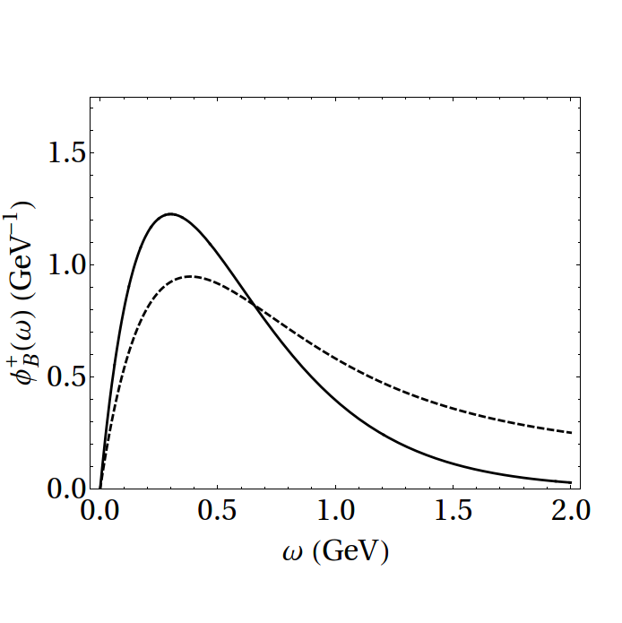
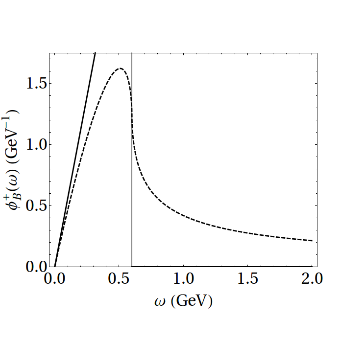
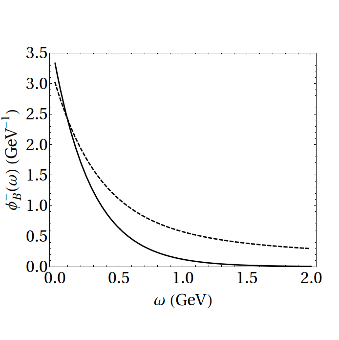
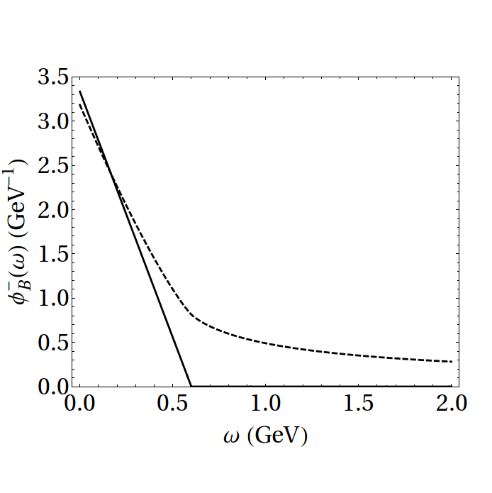
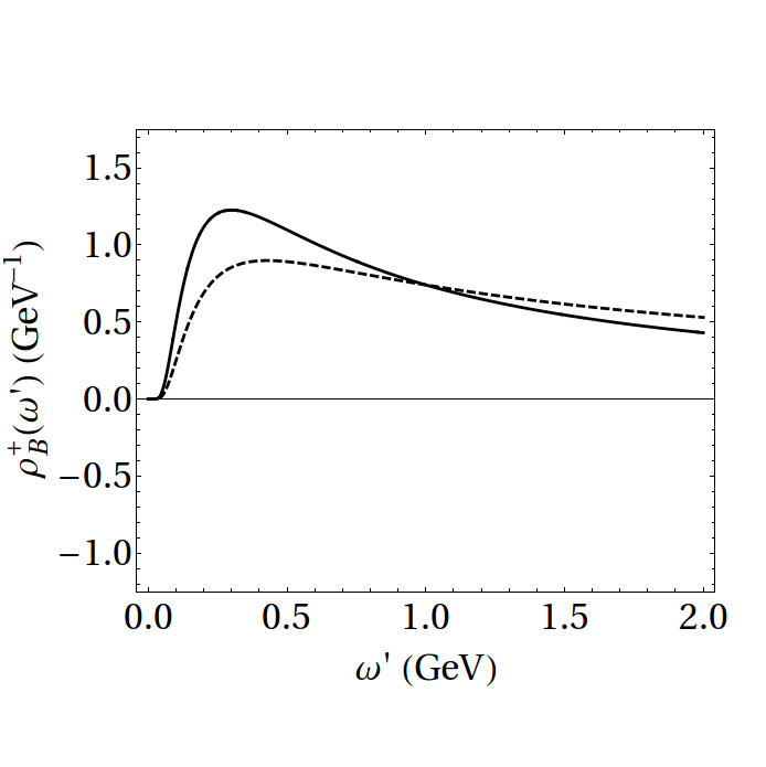
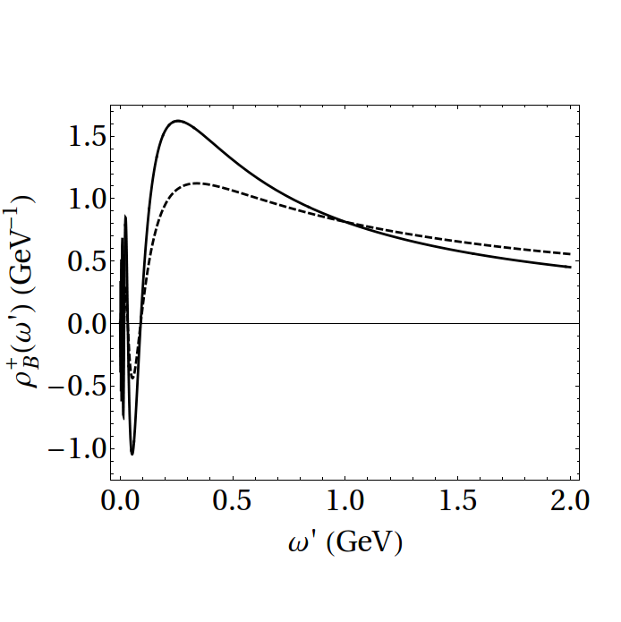
Figure 1: Left: exponential model from (60) showing the LCDAs $\phi_{B}^{+}(\omega)$ (top), $\phi_{B}^{-}(\omega)$ (center) and the spectral function $\rho_{B}^{+}(\omega^{\prime})$ (bottom), using $\mu_{0}=1$ GeV and $\omega_{0}=0.3$ GeV as input (solid line) and evolving to another scale corresponding to $g=0.3$ (dashed line) and neglecting the overall factor $e^{V-2\gamma_{E}g}$ for simplicity. Right: the same for the free parton model (62) with $\bar{\Lambda}=0.3$ GeV.

2.2.2 Corrections to Wandzura-Wilczek Relation

Corrections to the WW approximation can be incorporated by abandoning the constraint ${\cal M}_{B}^{(2)}\not{k}=0$ from the light quark’s Dirac equation. We thus write a more general ansatz,

$${\cal M}_{B}^{(2)}(v,k) =-\frac{i\tilde{f}_{B}m_{B}}{4}\left[(1+\not{v})\left\{\not{k}\,\psi_{B1}(x)+x\,\psi_{B2}(x)\right\}\gamma_{5}\right]\,.$$ (64)

Considering again the convolution with an appropriate hard-scattering kernel, one has

$$\int\widetilde{dk}\,{\rm tr}\left[\left(T_{0}(\omega)+k_{\perp}^{\mu}T_{\mu}(\omega)\right){\cal M}_{B}^{(2)}(v,k)\right]$$ (65)

$$= -\frac{i\tilde{f}_{B}m_{B}}{4}\,{\rm tr}\left[\int d\omega\,T_{0}(\omega)\,\int dx\,\psi_{B1}(x)\,\frac{1+\not{v}}{2}\left(\omega\not{n}_{+}+(x-\omega)\,\not{n}_{-}\right)\gamma_{5}\right]$$ (66)

$$-\frac{i\tilde{f}_{B}m_{B}}{4}\,{\rm tr}\left[\int d\omega\,T_{0}(\omega)\,\int dx\,\psi_{B2}(x)\,\frac{1+\not{v}}{2}\left(x\,\not{n}_{+}+x\,\not{n}_{-}\right)\gamma_{5}\right]$$ (67)

$$-\frac{i\tilde{f}_{B}m_{B}}{4}\,{\rm tr}\left[\int d\omega\,T_{\mu}(\omega)\,\int dx\,\psi_{B1}(x)\,\frac{1+\not{v}}{2}\left(-\omega\,(x-\omega)\,\gamma_{\perp}^{\mu}\right)\gamma_{5}\right]\,.$$ (68)

The LCDAs for this ansatz follow as

$$\phi_{B}^{+}(\omega) =\int_{\omega}^{\infty}dx\left\{\omega\,\psi_{B1}(x)+x\,\psi_{B2}(x)\right\}\,,$$ (69)

$$\phi_{B}^{-}(\omega) =\int_{\omega}^{\infty}dx\,\left\{(x-\omega)\,\psi_{B1}(x)+x\,\psi_{B2}(x)\right\}\,,$$ (70)

together with

$$\omega\,\phi_{B}^{-}(\omega)-\int_{0}^{\omega}d\eta\left(\phi_{B}^{-}(\eta)-\phi_{B}^{+}(\eta)\right) =\omega\,\int_{\omega}^{\infty}dx\,x\,\psi_{B2}(x)\,.$$ (71)

The wave function $\psi_{B2}(x)$ can thus be reconstructed from integrals of the 3-particle LCDAs $(\Psi_{A}-\Psi_{V})$ using (10), and vice versa.

2.2.3 Higher Fock States

Our formalism can also be applied to construct on-shell wave functions for higher Fock states. As an example, we will consider the quark-antiquark-gluon contribution in the WW approximation. We recall that the partonic Fock-state interpretation refers to light-cone gauge $n_{-}A(x)=0$, which we will assume in the following. For the 3-particle contributions, it is for practical purposes often sufficient to consider convolutions with a hard-scattering kernel that does not depend on any transverse momenta. To keep the discussion simple, we will therefore focus on the strict collinear limit, i.e. we will assume a corresponding hard-scattering kernel without the linear terms in partonic transverse momenta.

The conventional definition of 3-particle LCDAs starts from the position-space matrix element Kawamura:2001jm (see also Geyer:2005fb ; Huang:2005kk )

$$z_{\nu}\,\langle 0|\bar{q}^{\beta}(z)\,[z,uz]\,gG^{\mu\nu}(uz)\,[uz,0]\,h_{v}^{\alpha}(0)|\bar{B}(v)\rangle$$ (72)

$$=\frac{\tilde{f}_{B}m_{B}}{2}\left[\frac{1+\not{v}}{2}\bigg{\{}(v^{\mu}\not{z}-t\gamma^{\mu})\,\big{(}\tilde{\Psi}_{A}(t,u)-\tilde{\Psi}_{V}(t,u)\big{)}\right.$$ (73)

$$\hskip 88.2037pt\left.-i\sigma^{\mu\nu}z_{\nu}\tilde{\Psi}_{V}(t,u)-z^{\mu}\tilde{X}_{A}(t,u)+\frac{z^{\mu}}{t}\not{z}\tilde{Y}_{A}(t,u)\bigg{\}}\gamma_{5}\right]^{\alpha\beta},$$ (74)

with $t=v\cdot z$. In order to relate this representation to the wave-function approach, we need the momentum-space projector corresponding to the non-local matrix element

$$\langle 0|\bar{q}^{\beta}(z)\,g\,A^{\mu}(uz)\,h_{v}^{\alpha}(0)|\bar{B}(v)\rangle$$ (75)

in light-cone gauge. In the collinear approximation, we further have $z^{\mu}=\tau n_{-}^{\mu}$, such that $t=\tau$ in a frame where $(v\cdot n_{-})=1$. We then obtain

$${\cal M}_{B}^{(3)}{}^{\mu}(v,\omega,\xi)=-{i\over\xi}\,\frac{\tilde{f}_{B}m_{B}}{2}\left[\frac{1+\not{v}}{2}\bigg{\{}(n_{-}^{\mu}\not{n}_{-}-n_{-}^{\mu}-\gamma_{\perp}^{\mu})\big{(}\Psi_{A}(\omega,\xi)-\Psi_{V}(\omega,\xi)\big{)}\right.$$ (76)

$$\hskip 31.2982pt\left.+(n_{-}^{\mu}\not{n}_{-}-n_{-}^{\mu}+\gamma_{\perp}^{\mu}\not{n}_{-})\Psi_{V}(\omega,\xi)-n_{-}^{\mu}X_{A}(\omega,\xi)+n_{-}^{\mu}\not{n}_{-}Y_{A}(\omega,\xi)\bigg{\}}\gamma_{5}\right]\,,$$ (77)

where we introduced the Fourier-transformed LCDAs

$$\Psi_{A}(\omega,\xi) =\int\frac{d\tau}{2\pi}\,\int\frac{du}{2\pi}\;\tau\,e^{i(\omega+\xi u)\tau}\,\tilde{\Psi}_{A}(\tau,u)\,,\qquad\text{etc.}$$ (78)

Proceeding in analogy to the 2-particle construction, we may formulate an equivalent representation of the momentum-space projector starting from on-shell momenta for the Fock-state components ($k^{\mu}$ with $k^{2}=0$ for the light anti-quark, $l^{\mu}$ with $l^{2}=0$ for the gluon, and $m_{b}v^{\mu}$ with $v^{2}=1$ for the heavy quark). The most general ansatz that fulfills the equations of motion for all constituents,

$$(\not{v}-1)\,{\cal M}_{B}^{(3)}{}^{\mu}={\cal M}_{B}^{(3)}{}^{\mu}\,\not{k}={\cal M}_{B}^{(3)}{}^{\mu}\,l_{\mu}=0\,,$$ (79)

is given by

$${\cal M}_{B}^{(3)}{}^{\mu}(v,k,l) =-i\,\frac{\tilde{f}_{B}m_{B}}{2}\;(1+\not{v})\,\bigg{\{}yk^{\mu}\Phi_{1}(x,y)+xl^{\mu}\Phi_{2}(x,y)+x\big{(}y\gamma^{\mu}-2v^{\mu}\not{l}\big{)}\Phi_{3}(x,y)$$ (80)

$$\hskip 28.45274pt+k^{\mu}\not{l}\Phi_{4}(x,y)+l^{\mu}\not{l}\Phi_{5}(x,y)+x\big{(}\gamma^{\mu}\not{l}-\not{l}\gamma^{\mu}\big{)}\Phi_{6}(x,y)\bigg{\}}\,\not{k}\gamma_{5}\,.$$ (81)

In general, the wave functions $\Phi_{i}$ depend on three invariants, $x=2\,v\cdot k$, $y=2\,v\cdot l$ and $z=2\,k\cdot l$, but in the above decomposition we have neglected the invariant mass of the antiquark-gluon subsystem, $z=(k+l)^{2}\simeq 0$, for simplicity, which is based on the assumption that the wave functions only depend on the total invariant mass of the partonic configuration, $(m_{b}v+k+l)^{2}\simeq m_{b}^{2}+m_{b}(x+y)$. Writing

$$k^{\mu}=\omega\,\frac{n_{+}^{\mu}}{2}+k_{\perp}^{\mu}+\frac{|k_{\perp}|^{2}}{\omega}\,\frac{n_{-}^{\mu}}{2}\,,\qquad\quad l^{\mu}=\xi\,\frac{n_{+}^{\mu}}{2}+l_{\perp}^{\mu}+\frac{|l_{\perp}|^{2}}{\xi}\,\frac{n_{-}^{\mu}}{2}\,,$$ (82)

which implies $x=\omega+|k_{\perp}|^{2}/\omega$ and $y=\xi+|l_{\perp}|^{2}/\xi$, we may neglect any odd powers of $k_{\perp}$ and $\l_{\perp}$ in the transverse-momentum integrals with a hard-scattering kernel. In light-cone coordinates, the momentum-space projector (81) may then be rewritten in terms of six independent structures, which we choose as

$$n_{-}^{\mu}\,,\ n_{+}^{\mu}\,,\ \gamma_{\perp}^{\mu}\,,\ n_{-}^{\mu}\not{n}_{-}\,,\ n_{+}^{\mu}\not{n}_{-}\,,\ \gamma_{\perp}^{\mu}\not{n}_{-}\,.$$ (83)

The light-cone gauge condition, ${\cal M}_{B}^{(3)}{}^{\mu}\,{n_{-}}_{\mu}=0$, further eliminates the $n_{+}^{\mu}$ and $n_{+}^{\mu}\not{n}_{-}$ structures (we use these constraints to determine $\Phi_{1}$ and $\Phi_{4}$). The remaining four Lorentz structures are of the form (77), and we can read off

$$\Psi_{A}(\omega,\xi)-\Psi_{V}(\omega,\xi)=\xi\,\int_{\omega}^{\infty}dx\int_{\xi}^{\infty}dy\bigg{\{}\xi(\omega-x)x\,\Phi_{2}(x,y)+2\big{(}\omega y-\xi(\omega-x)\big{)}x\,\Phi_{3}(x,y)$$ (84)

$$\hskip 28.45274pt+\xi\big{(}(\omega-x)\xi+(\xi-y)\omega\big{)}\,\Phi_{5}(x,y)+2\big{(}(\omega-x)\xi+2(\xi-y)\omega\big{)}x\,\Phi_{6}(x,y)\bigg{\}}\,,$$ (85)

$$\Psi_{V}(\omega,\xi)={\xi\over 2}\,\int_{\omega}^{\infty}dx\int_{\xi}^{\infty}dy\bigg{\{}2x(x(y-2\xi)+2\omega(\xi-y))\,\Phi_{3}(x,y)$$ (86)

$$\hskip 28.45274pt+\xi(\omega(3y-4\xi)+x(3\xi-2y))\,\Phi_{5}(x,y)+4x\omega(y-\xi)\,\Phi_{6}(x,y)\bigg{\}}\,,$$ (87)

$$\Psi_{A}(\omega,\xi)+X_{A}(\omega,\xi)=\xi\,\int_{\omega}^{\infty}dx\int_{\xi}^{\infty}dy\bigg{\{}x(\xi x-y\omega)\,\Phi_{2}(x,y)-(y-\xi)(y\omega-\xi x)\,\Phi_{5}(x,y)$$ (88)

$$\hskip 28.45274pt+2x\big{(}\xi(x-\omega)+\omega(y-\xi)\big{)}\,\left(\Phi_{3}(x,y)-\Phi_{6}(x,y)\right)\bigg{\}}\,,$$ (89)

$$\Psi_{A}(\omega,\xi)+Y_{A}(\omega,\xi)=-{\xi\over 2\omega}\,\int_{\omega}^{\infty}dx\int_{\xi}^{\infty}dy\bigg{\{}x(x-2\omega)(\xi x-y\omega)\,\Phi_{2}(x,y)$$ (90)

$$\hskip 28.45274pt+\big{(}\xi x-y\omega\big{)}^{2}\,\Phi_{5}(x,y)-2x^{2}\big{(}\xi(x-\omega)+\omega(y-\xi)\big{)}\,\left(\Phi_{3}(x,y)-\Phi_{6}(x,y)\right)\bigg{\}}\,.$$ (91)

In the collinear approximation, the four 3-particle LCDAs $\Psi_{A},\Psi_{V},X_{A}$ and $Y_{A}$ can thus be expressed through four independent on-shell wave functions.

3 $\Lambda_{b}$–Baryons

3.1 Light-Cone Distribution Amplitudes

Light-cone distribution amplitudes for $\Lambda_{b}$-baryons in HQET have been classified in Ball:2008fw (for related work, see also Ali:2012pn ). They contain the hadronic information entering factorization theorems for exclusive $\Lambda_{b}$ transitions in the heavy-quark limit (see e.g. Feldmann:2011xf ; Wang:2009hra ). In this work, we will focus on the LCDAs related to the leading 3-particle operators Ball:2008fw (gauge-links are understood implicitly, but not shown for simplicity),

$$\epsilon^{abc}\,\langle 0|\left(u^{a}(\tau_{1}n_{-})\,C\gamma_{5}\,\not{n}_{-}\,d^{b}(\tau_{2}n_{-})\right)h_{v}^{c}(0)|\Lambda_{b}(v,s)\rangle =f_{\Lambda_{b}}^{(2)}\,\tilde{\phi}_{2}(\tau_{1},\tau_{2})\,u_{\Lambda_{b}}(v,s)\,,$$ (92)

$$\epsilon^{abc}\,\langle 0|\left(u^{a}(\tau_{1}n_{-})\,C\gamma_{5}\,\not{n}_{+}\,d^{b}(\tau_{2}n_{-})\right)h_{v}^{c}(0)|\Lambda_{b}(v,s)\rangle =f_{\Lambda_{b}}^{(2)}\,\tilde{\phi}_{4}(\tau_{1},\tau_{2})\,u_{\Lambda_{b}}(v,s)\,,$$ (93)

for the chiral-odd part (i.e. with an odd number of Dirac matrices in the light-diquark current), and

$$\epsilon^{abc}\,\langle 0|\left(u^{a}(\tau_{1}n_{-})\,C\gamma_{5}\,d^{b}(\tau_{2}n_{-})\right)h_{v}^{c}(0)|\Lambda_{b}(v,s)\rangle =f_{\Lambda_{b}}^{(1)}\,\tilde{\phi}_{3}^{s}(\tau_{1},\tau_{2})\,u_{\Lambda_{b}}(v,s)\,,$$ (94)

$$\epsilon^{abc}\,\langle 0|\left(u^{a}(\tau_{1}n_{-})\,C\gamma_{5}\,i\sigma_{\mu\nu}n_{+}^{\mu}n_{-}^{\nu}\,d^{b}(\tau_{2}n_{-})\right)h_{v}^{c}(0)|\Lambda_{b}(v,s)\rangle =2\,f_{\Lambda_{b}}^{(1)}\,\tilde{\phi}_{3}^{\sigma}(\tau_{1},\tau_{2})\,u_{\Lambda_{b}}(v,s)\,,$$ (95)

for the chiral-even part. Here $u_{\Lambda_{b}}(v,s)$ denotes the on-shell Dirac spinor for the $\Lambda_{b}$-baryon, and the prefactors $f_{\Lambda_{b}}^{(1,2)}$ are defined by the normalization of the matrix elements of the corresponding local operators in HQET at a given renormalization scale.

3.1.1 Light-Cone Projectors for 3-Particle Fock State

The above definitions can be cast into a manifestly Lorentz-invariant form by defining the most general non-local matrix elements in coordinate space as Feldmann:2011xf

$$\epsilon^{abc}\,\langle 0|\left(u^{a}_{\alpha}(z_{1})\,d^{b}_{\beta}(z_{2})\right)h^{c}_{v}(0)|\Lambda_{b}(v,s)\rangle$$ (96)

$$\equiv \frac{1}{4}\left\{f^{(1)}_{\Lambda_{b}}\left[\tilde{M}^{(1)}(v,z_{1},z_{2})\gamma_{5}C^{T}\right]_{\beta\alpha}+f^{(2)}_{\Lambda_{b}}\left[\tilde{M}^{(2)}(v,z_{1},z_{2})\gamma_{5}C^{T}\right]_{\beta\alpha}\right\}u_{\Lambda_{b}}(v,s)\,,$$ (97)

with a part that contains an odd number of Dirac matrices ($t_{i}=v\cdot z_{i}$),

$$\tilde{M}^{(2)}(v,z_{1},z_{2}) =\hbox to0.0pt{\hbox to5.20601pt{\hfil/\hfil}\hss}v\,\tilde{\Phi}_{2}(t_{1},t_{2},z_{1}^{2},z_{2}^{2},z_{1}\cdot z_{2})+\frac{\tilde{\Phi}_{X}(t_{1},t_{2},z_{1}^{2},z_{2}^{2},z_{1}\cdot z_{2})}{4t_{1}t_{2}}\left(\hbox to0.0pt{\hbox to5.0903pt{\hfil/\hfil}\hss}z_{2}\hbox to0.0pt{\hbox to5.20601pt{\hfil/\hfil}\hss}v\hbox to0.0pt{\hbox to5.0903pt{\hfil/\hfil}\hss}z_{1}-\hbox to0.0pt{\hbox to5.0903pt{\hfil/\hfil}\hss}z_{1}\hbox to0.0pt{\hbox to5.20601pt{\hfil/\hfil}\hss}v\hbox to0.0pt{\hbox to5.0903pt{\hfil/\hfil}\hss}z_{2}\right)$$ (98)

$$\quad+\frac{\tilde{\Phi}_{42}^{(i)}(t_{1},t_{2},z_{1}^{2},z_{2}^{2},z_{1}\cdot z_{2})}{2t_{1}}\,\hbox to0.0pt{\hbox to5.0903pt{\hfil/\hfil}\hss}z_{1}+\frac{\tilde{\Phi}_{42}^{(ii)}(t_{1},t_{2},z_{1}^{2},z_{2}^{2},z_{1}\cdot z_{2})}{2t_{2}}\,\hbox to0.0pt{\hbox to5.0903pt{\hfil/\hfil}\hss}z_{2}\,,$$ (99)

(100)

and a part that contains an even number of Dirac matrices,

$$\tilde{M}^{(1)}(v,z_{1},z_{2}) =\tilde{\Phi}_{3}^{(0)}(t_{1},t_{2},z_{1}^{2},z_{2}^{2},z_{1}\cdot z_{2})+\frac{\tilde{\Phi}_{Y}(t_{1},t_{2},z_{1}^{2},z_{2}^{2},z_{1}\cdot z_{2})}{4t_{1}t_{2}}\left(\hbox to0.0pt{\hbox to5.0903pt{\hfil/\hfil}\hss}z_{2}\hbox to0.0pt{\hbox to5.0903pt{\hfil/\hfil}\hss}z_{1}-\hbox to0.0pt{\hbox to5.0903pt{\hfil/\hfil}\hss}z_{1}\hbox to0.0pt{\hbox to5.0903pt{\hfil/\hfil}\hss}z_{2}\right)$$ (101)

$$\quad+\frac{\tilde{\Phi}_{3}^{(i)}(t_{1},t_{2},z_{1}^{2},z_{2}^{2},z_{1}\cdot z_{2})}{2t_{1}}\,\hbox to0.0pt{\hbox to5.20601pt{\hfil/\hfil}\hss}v\hbox to0.0pt{\hbox to5.0903pt{\hfil/\hfil}\hss}z_{1}+\frac{\tilde{\Phi}_{3}^{(ii)}(t_{1},t_{2},z_{1}^{2},z_{2}^{2},z_{1}\cdot z_{2})}{2t_{2}}\,\hbox to0.0pt{\hbox to5.0903pt{\hfil/\hfil}\hss}z_{2}\hbox to0.0pt{\hbox to5.20601pt{\hfil/\hfil}\hss}v\,.$$ (102)

(103)

Considering isospin invariance for the light-quark fields (exchanging $z_{1}\leftrightarrow z_{2}$ and taking care of the charge-conjugation properties of the Dirac matrices), one obtains the following relations between the individual functions,

$$\tilde{\Phi}_{2}(t_{1},t_{2},z_{1}^{2},z_{2}^{2},z_{1}\cdot z_{2}) =\tilde{\Phi}_{2}(t_{2},t_{1},z_{2}^{2},z_{1}^{2},z_{1}\cdot z_{2})\,,$$ (104)

$$\tilde{\Phi}_{42}^{(i)}(t_{1},t_{2},z_{1}^{2},z_{2}^{2},z_{1}\cdot z_{2}) =\tilde{\Phi}_{42}^{(ii)}(t_{2},t_{1},z_{2}^{2},z_{1}^{2},z_{1}\cdot z_{2})\,,$$ (105)

$$\tilde{\Phi}_{X}(t_{1},t_{2},z_{1}^{2},z_{2}^{2},z_{1}\cdot z_{2}) =\tilde{\Phi}_{X}(t_{2},t_{1},z_{2}^{2},z_{1}^{2},z_{1}\cdot z_{2})\,,$$ (106)

and

$$\tilde{\Phi}_{3}^{(0)}(t_{1},t_{2},z_{1}^{2},z_{2}^{2},z_{1}\cdot z_{2}) =\tilde{\Phi}_{3}^{(0)}(t_{2},t_{1},z_{2}^{2},z_{1}^{2},z_{1}\cdot z_{2})\,,$$ (107)

$$\tilde{\Phi}_{3}^{(i)}(t_{1},t_{2},z_{1}^{2},z_{2}^{2},z_{1}\cdot z_{2}) =\tilde{\Phi}_{3}^{(ii)}(t_{2},t_{1},z_{2}^{2},z_{1}^{2},z_{1}\cdot z_{2})\,,$$ (108)

$$\tilde{\Phi}_{Y}(t_{1},t_{2},z_{1}^{2},z_{2}^{2},z_{1}\cdot z_{2}) =\tilde{\Phi}_{Y}(t_{2},t_{1},z_{2}^{2},z_{1}^{2},z_{1}\cdot z_{2})\,.$$ (109)

3.1.2 The Chiral-Odd Projector $\tilde{M}^{(2)}$

In the same way as we argued for $B$-mesons, we may again expand the arguments $z_{1}$ and $z_{2}$ around the light-cone, such that $(n_{-}z_{i})\ll z_{i}^{\perp}\ll(n_{+}z_{i})$, to obtain the projector in coordinate-space as

$$\tilde{M}^{(2)}(v,z_{1},z_{2}) \longrightarrow\frac{\hbox to0.0pt{\hbox to6.00235pt{\hfil/\hfil}\hss}n_{+}}{2}\,\tilde{\phi}_{2}(\tau_{1},\tau_{2})+\frac{\hbox to0.0pt{\hbox to6.00235pt{\hfil/\hfil}\hss}n_{-}}{2}\left(\tilde{\phi}_{2}(\tau_{1},\tau_{2})+\tilde{\phi}_{42}^{(i)}(\tau_{1},\tau_{2})+\tilde{\phi}_{42}^{(ii)}(\tau_{1},\tau_{2})\right)$$ (110)

$$\quad+\frac{\tilde{\phi}_{42}^{(i)}(\tau_{1},\tau_{2})}{2\tau_{1}}\,\hbox to0.0pt{\hbox to5.0903pt{\hfil/\hfil}\hss}z_{1}^{\perp}+\frac{\tilde{\phi}_{42}^{(ii)}(\tau_{1},\tau_{2})}{2\tau_{2}}\,\hbox to0.0pt{\hbox to5.0903pt{\hfil/\hfil}\hss}z_{2}^{\perp}$$ (111)

$$\quad+\tilde{\phi}_{X}(\tau_{1},\tau_{2})\left(\frac{\hbox to0.0pt{\hbox to5.0903pt{\hfil/\hfil}\hss}z_{1}^{\perp}}{2\tau_{1}}-\frac{\hbox to0.0pt{\hbox to5.0903pt{\hfil/\hfil}\hss}z_{2}^{\perp}}{2\tau_{2}}\right)\left(\frac{\hbox to0.0pt{\hbox to6.00235pt{\hfil/\hfil}\hss}n_{-}\hbox to0.0pt{\hbox to6.00235pt{\hfil/\hfil}\hss}n_{+}}{4}-\frac{\hbox to0.0pt{\hbox to6.00235pt{\hfil/\hfil}\hss}n_{+}\hbox to0.0pt{\hbox to6.00235pt{\hfil/\hfil}\hss}n_{-}}{4}\right)+{\cal O}(z_{i\perp}^{2},n_{-}z_{i})\,.$$ (112)

Here again we denote with $\tau_{i}=\frac{n_{+}z_{i}}{2}$ the Fourier-conjugate variables to the momentum components $\omega_{i}=(n_{-}k_{i})$ of the associated light-quark states in the heavy baryon, such that

$$\phi_{2}(\omega_{1},\omega_{2}) \equiv\int\frac{d\tau_{1}}{2\pi}\,e^{i\omega_{1}\tau_{1}}\,\int\frac{d\tau_{2}}{2\pi}\,e^{i\omega_{2}\tau_{2}}\,\tilde{\phi}_{2}(\tau_{1},\tau_{2})\qquad\mbox{etc.}$$ (113)

Comparison with the definition in (93) yields the relation

$$\tilde{\phi}_{42}^{(i)}(\tau_{1},\tau_{2})+\tilde{\phi}_{42}^{(ii)}(\tau_{1},\tau_{2}) =\tilde{\phi}_{4}(\tau_{1},\tau_{2})-\tilde{\phi}_{2}(\tau_{1},\tau_{2})\,,$$ (114)

while the asymmetric combination of $\tilde{\phi}_{42}^{(i)}$ and $\tilde{\phi}_{42}^{(ii)}$, as well as $\tilde{\phi}_{X}$ do not contribute in the collinear limit $z_{i}^{2}\to 0$. After Fourier transformation, the general momentum-space representation for (112) including the first-order terms off the light-cone becomes

$$M^{(2)}(\omega_{1},\omega_{2})= \ \frac{\hbox to0.0pt{\hbox to6.00235pt{\hfil/\hfil}\hss}n_{+}}{2}\,\phi_{2}(\omega_{1},\omega_{2})+\frac{\hbox to0.0pt{\hbox to6.00235pt{\hfil/\hfil}\hss}n_{-}}{2}\,\phi_{4}(\omega_{1},\omega_{2})$$ (115)

$$-\frac{1}{2}\,\gamma_{\mu}^{\perp}\,\int_{0}^{\omega_{1}}d\eta_{1}\left(\phi_{42}^{(i)}(\eta_{1},\omega_{2})-\phi_{X}(\eta_{1},\omega_{2})\right)\frac{\hbox to0.0pt{\hbox to6.00235pt{\hfil/\hfil}\hss}n_{+}\hbox to0.0pt{\hbox to6.00235pt{\hfil/\hfil}\hss}n_{-}}{4}\,\frac{\partial}{\partial k_{1\mu}^{\perp}}$$ (116)

$$-\frac{1}{2}\,\gamma_{\mu}^{\perp}\,\int_{0}^{\omega_{1}}d\eta_{1}\left(\phi_{42}^{(i)}(\eta_{1},\omega_{2})+\phi_{X}(\eta_{1},\omega_{2})\right)\frac{\hbox to0.0pt{\hbox to6.00235pt{\hfil/\hfil}\hss}n_{-}\hbox to0.0pt{\hbox to6.00235pt{\hfil/\hfil}\hss}n_{+}}{4}\,\frac{\partial}{\partial k_{1\mu}^{\perp}}$$ (117)

$$-\frac{1}{2}\,\gamma_{\mu}^{\perp}\,\int_{0}^{\omega_{2}}d\eta_{2}\left(\phi_{42}^{(ii)}(\omega_{1},\eta_{2})-\phi_{X}(\omega_{1},\eta_{2})\right)\frac{\hbox to0.0pt{\hbox to6.00235pt{\hfil/\hfil}\hss}n_{-}\hbox to0.0pt{\hbox to6.00235pt{\hfil/\hfil}\hss}n_{+}}{4}\,\frac{\partial}{\partial k_{2\mu}^{\perp}}$$ (118)

$$-\frac{1}{2}\,\gamma_{\mu}^{\perp}\,\int_{0}^{\omega_{2}}d\eta_{2}\left(\phi_{42}^{(ii)}(\omega_{1},\eta_{2})+\phi_{X}(\omega_{1},\eta_{2})\right)\frac{\hbox to0.0pt{\hbox to6.00235pt{\hfil/\hfil}\hss}n_{+}\hbox to0.0pt{\hbox to6.00235pt{\hfil/\hfil}\hss}n_{-}}{4}\,\frac{\partial}{\partial k_{2\mu}^{\perp}}\,.$$ (119)

Compared to the mesonic analogue, we observe that a larger number of independent terms that are sensitive to the transverse momenta of the light quarks in the hard-scattering kernel appear.

3.1.3 The Chiral-Even Projector $\tilde{M}^{(1)}$

Similarly, for the chiral-even projector we obtain the expansion around the collinear limit as

$$\tilde{M}^{(1)}(v,z_{1},z_{2}) \longrightarrow\tilde{\phi}_{3}^{(0)}(\tau_{1},\tau_{2})+\tilde{\phi}_{3}^{(i)}(\tau_{1},\tau_{2})\,\frac{\hbox to0.0pt{\hbox to6.00235pt{\hfil/\hfil}\hss}n_{+}\hbox to0.0pt{\hbox to6.00235pt{\hfil/\hfil}\hss}n_{-}}{4}+\tilde{\phi}_{3}^{(ii)}(\tau_{1},\tau_{2})\,\frac{\hbox to0.0pt{\hbox to6.00235pt{\hfil/\hfil}\hss}n_{-}\hbox to0.0pt{\hbox to6.00235pt{\hfil/\hfil}\hss}n_{+}}{4}$$ (120)

$$\quad+\tilde{\phi}_{3}^{(i)}(\tau_{1},\tau_{2})\,\frac{\hbox to0.0pt{\hbox to5.20601pt{\hfil/\hfil}\hss}v\hbox to0.0pt{\hbox to5.0903pt{\hfil/\hfil}\hss}z_{1}^{\perp}}{2\tau_{1}}+\tilde{\phi}_{3}^{(ii)}(\tau_{1},\tau_{2})\,\frac{\hbox to0.0pt{\hbox to5.0903pt{\hfil/\hfil}\hss}z_{2}^{\perp}\hbox to0.0pt{\hbox to5.20601pt{\hfil/\hfil}\hss}v}{2\tau_{2}}$$ (121)

$$\quad+\tilde{\phi}_{Y}(\tau_{1},\tau_{2})\left(\frac{\hbox to0.0pt{\hbox to5.0903pt{\hfil/\hfil}\hss}z_{2}^{\perp}\hbox to0.0pt{\hbox to6.00235pt{\hfil/\hfil}\hss}n_{-}}{2\tau_{2}}+\frac{\hbox to0.0pt{\hbox to6.00235pt{\hfil/\hfil}\hss}n_{-}\hbox to0.0pt{\hbox to5.0903pt{\hfil/\hfil}\hss}z_{1}^{\perp}}{2\tau_{1}}\right)+{\cal O}(z_{i\perp}^{2},n_{-}z_{i})\,,$$ (122)

where now from the comparison with (95) one has the relations

$$\tilde{\phi}_{3}^{s}(\tau_{1},\tau_{2}) =\frac{2\tilde{\phi}_{3}^{(0)}(\tau_{1},\tau_{2})+\tilde{\phi}_{3}^{(i)}(\tau_{1},\tau_{2})+\tilde{\phi}_{3}^{(ii)}(\tau_{1},\tau_{2})}{2}\,,$$ (123)

$$\tilde{\phi}_{3}^{\sigma}(\tau_{1},\tau_{2}) =\frac{\tilde{\phi}_{3}^{(ii)}(\tau_{1},\tau_{2})-\tilde{\phi}_{3}^{(i)}(\tau_{1},\tau_{2})}{2}\,.$$ (124)

It is sometimes more convenient to define symmetric and antisymmetric combinations of the functions $\phi_{3}^{s}$ and $\phi_{3}^{\sigma}$ which will be denoted as Ball:2008fw

$$\tilde{\phi}_{3}^{+-}(\tau_{1},\tau_{2}) =2\left(\tilde{\phi}_{3}^{s}(\tau_{1},\tau_{2})+\tilde{\phi}_{3}^{\sigma}(\tau_{1},\tau_{2})\right)=2\left(\tilde{\phi}_{3}^{(0)}(\tau_{1},\tau_{2})+\tilde{\phi}_{3}^{(ii)}(\tau_{1},\tau_{2})\right)\,,$$ (125)

$$\tilde{\phi}_{3}^{-+}(\tau_{1},\tau_{2}) =2\left(\tilde{\phi}_{3}^{s}(\tau_{1},\tau_{2})-\tilde{\phi}_{3}^{\sigma}(\tau_{1},\tau_{2})\right)=2\left(\tilde{\phi}_{3}^{(0)}(\tau_{1},\tau_{2})+\tilde{\phi}_{3}^{(i)}(\tau_{1},\tau_{2})\right)\,.$$ (126)

The expansion of the corresponding momentum-space projector then takes the general form

$$M^{(1)}(\omega_{1},\omega_{2})= \ \frac{\hbox to0.0pt{\hbox to6.00235pt{\hfil/\hfil}\hss}n_{-}\hbox to0.0pt{\hbox to6.00235pt{\hfil/\hfil}\hss}n_{+}}{8}\,\phi_{3}^{+-}(\omega_{1},\omega_{2})+\frac{\hbox to0.0pt{\hbox to6.00235pt{\hfil/\hfil}\hss}n_{+}\hbox to0.0pt{\hbox to6.00235pt{\hfil/\hfil}\hss}n_{-}}{8}\,\phi_{3}^{-+}(\omega_{1},\omega_{2})$$ (127)

$$-\frac{1}{2}\,\int_{0}^{\omega_{1}}d\eta_{1}\,\phi_{3}^{(i)}(\eta_{1},\omega_{2})\,\hbox to0.0pt{\hbox to5.20601pt{\hfil/\hfil}\hss}v\,\gamma_{\mu}^{\perp}\,\frac{\partial}{\partial k_{1\mu}^{\perp}}-\frac{1}{2}\,\int_{0}^{\omega_{2}}d\eta_{2}\,\phi_{3}^{(ii)}(\omega_{1},\eta_{2})\,\gamma_{\mu}^{\perp}\,\hbox to0.0pt{\hbox to5.20601pt{\hfil/\hfil}\hss}v\,\frac{\partial}{\partial k_{2\mu}^{\perp}}$$ (128)

$$-\frac{1}{2}\,\int_{0}^{\omega_{1}}d\eta_{1}\,\phi_{Y}(\eta_{1},\omega_{2})\,\hbox to0.0pt{\hbox to6.00235pt{\hfil/\hfil}\hss}n_{-}\gamma_{\mu}^{\perp}\,\frac{\partial}{\partial k_{1\mu}^{\perp}}-\frac{1}{2}\,\int_{0}^{\omega_{2}}d\eta_{2}\,\phi_{Y}(\omega_{1},\eta_{2})\,\gamma_{\mu}^{\perp}\,\hbox to0.0pt{\hbox to6.00235pt{\hfil/\hfil}\hss}n_{-}\frac{\partial}{\partial k_{2\mu}^{\perp}}\,.$$ (129)

(130)

Again, in the general case, it involves four independent structures related to transverse momenta of the light quarks.

3.1.4 Wandzura-Wilczek Approximation

In the WW approximation, the matrices $\tilde{M}^{(1,2)}(z_{1},z_{2})$ fulfill the equations of motion for free quark fields,

$$\gamma_{\mu}\,i\partial_{2}^{\mu}\,\tilde{M}^{(1,2)}(v,z_{1},z_{2})=i\partial_{1}^{\mu}\,\tilde{M}^{(1,2)}(v,z_{1},z_{2})\,\gamma_{\mu}=0\,,$$ (131)

which translates into differential equations for the LCDAs in the collinear limit. These can be obtained by expanding the above equations around the light-cone, and solving for the derivatives with respect to the arguments $(z_{i}^{2},z_{1}\cdot z_{2})$ off the light cone. Alternatively, one can start from the expanded form of $\tilde{M}^{(1,2)}$ and consider the projected equations

$$\frac{\hbox to0.0pt{\hbox to6.00235pt{\hfil/\hfil}\hss}n_{+}\hbox to0.0pt{\hbox to6.00235pt{\hfil/\hfil}\hss}n_{-}}{4}\,\gamma_{\mu}\,i\partial_{2}^{\mu}\,\tilde{M}^{(1,2)}(v,z_{1},z_{2})\big{|}_{z_{1,2}^{\perp}=0}=i\partial_{1}^{\mu}\,\tilde{M}^{(1,2)}(v,z_{1},z_{2})\,\gamma_{\mu}\frac{\hbox to0.0pt{\hbox to6.00235pt{\hfil/\hfil}\hss}n_{-}\hbox to0.0pt{\hbox to6.00235pt{\hfil/\hfil}\hss}n_{+}}{4}\big{|}_{z_{1,2}^{\perp}=0}=0\,.$$ (132)

In both cases, this yields the following WW relations for the LCDAs in $\tilde{M}^{(2)}$,

$$\tilde{\phi}_{42}^{(i)}(\tau_{1},\tau_{2})+\tilde{\phi}_{X}(\tau_{1},\tau_{2})+\tau_{1}\,\frac{\partial}{\partial\tau_{1}}\,\tilde{\phi}_{4}(\tau_{1},\tau_{2})=0\,,$$ (133)

$$\tilde{\phi}_{42}^{(ii)}(\tau_{1},\tau_{2})+\tilde{\phi}_{X}(\tau_{1},\tau_{2})+\tau_{2}\,\frac{\partial}{\partial\tau_{2}}\,\tilde{\phi}_{4}(\tau_{1},\tau_{2})=0\,.$$ (134)

For the Fourier-transformed LCDAs this implies

$$\phi_{42}^{(i)}(\omega_{1},\omega_{2})+\phi_{X}(\omega_{1},\omega_{2})-\frac{\partial}{\partial\omega_{1}}\left(\omega_{1}\,\phi_{4}(\omega_{1},\omega_{2})\right)=0\,,$$ (135)

$$\phi_{42}^{(ii)}(\omega_{1},\omega_{2})+\phi_{X}(\omega_{1},\omega_{2})-\frac{\partial}{\partial\omega_{2}}\left(\omega_{2}\,\phi_{4}(\omega_{1},\omega_{2})\right)=0\,.$$ (136)

Equivalently, by considering linear combinations of the above, the following relations hold

$$\phi_{42}^{(i)}(\omega_{1},\omega_{2})-\phi_{42}^{(ii)}(\omega_{1},\omega_{2}) =\frac{\partial}{\partial\omega_{1}}\left(\omega_{1}\,\phi_{4}(\omega_{1},\omega_{2})\right)-\frac{\partial}{\partial\omega_{2}}\left(\omega_{2}\,\phi_{4}(\omega_{1},\omega_{2})\right)\,,$$ (137)

$$2\,\phi_{X}(\omega_{1},\omega_{2})+\phi_{4}(\omega_{1},\omega_{2})-\phi_{2}(\omega_{1},\omega_{2}) =\frac{\partial}{\partial\omega_{1}}\left(\omega_{1}\,\phi_{4}(\omega_{1},\omega_{2})\right)+\frac{\partial}{\partial\omega_{2}}\left(\omega_{2}\,\phi_{4}(\omega_{1},\omega_{2})\right)\,.$$ (138)

This reveals that, once the functions $\phi_{2}$ and $\phi_{4}$ – which are the relevant LCDAs in the collinear limit – are given, the function $\phi_{X}$ and the asymmetric combination of $\phi_{42}^{(i,ii)}$ can be calculated from the WW approximation.

In a similar way, for the LCDAs in $\tilde{M}^{(1)}$ we obtain the relations

$$\tilde{\phi}_{3}^{(i)}(\tau_{1},\tau_{2})+\tau_{1}\,\frac{\partial}{\partial\tau_{1}}\left(\tilde{\phi}_{3}^{(0)}(\tau_{1},\tau_{2})+\tilde{\phi}_{3}^{(i)}(\tau_{1},\tau_{2})\right) =0\,,$$ (139)

$$\tilde{\phi}_{3}^{(ii)}(\tau_{1},\tau_{2})+\tau_{2}\,\frac{\partial}{\partial\tau_{2}}\left(\tilde{\phi}_{3}^{(0)}(\tau_{1},\tau_{2})+\tilde{\phi}_{3}^{(ii)}(\tau_{1},\tau_{2})\right) =0\,,$$ (140)

or, in momentum space,

$$\phi_{3}^{(i)}(\omega_{1},\omega_{2})-\frac{\partial}{\partial\omega_{1}}\left(\omega_{1}\,\phi_{3}^{(0)}(\omega_{1},\omega_{2})+\omega_{1}\,\phi_{3}^{(i)}(\omega_{1},\omega_{2})\right) =0\,,$$ (141)

$$\phi_{3}^{(ii)}(\omega_{1},\omega_{2})-\frac{\partial}{\partial\omega_{2}}\left(\omega_{2}\,\phi_{3}^{(0)}(\omega_{1},\omega_{2})+\omega_{2}\,\phi_{3}^{(ii)}(\omega_{1},\omega_{2})\right) =0\,.$$ (142)

Notice that in this case, the function $\phi_{Y}$ does not appear in the WW relations, and therefore remains independent, whereas the functions $\phi_{3}^{+-}$ and $\phi_{3}^{-+}$ that are relevant in the collinear limit are related by

$$-\omega_{1}\,\frac{\partial}{\partial\omega_{1}}\,\phi_{3}^{-+}(\omega_{1},\omega_{2}) =-\omega_{2}\,\frac{\partial}{\partial\omega_{2}}\,\phi_{3}^{+-}(\omega_{1},\omega_{2})=2\,\phi_{3}^{(0)}(\omega_{1},\omega_{2})\,.$$ (143)

3.2 Construction from Momentum Space

We are now going to apply the same formalism that we have developed for $B$-mesons to construct momentum-space projectors for $\Lambda_{b}$-baryons from 3-particle wave functions. To keep the discussion simple, we will ignore corrections to the WW relation in the rest of the paper. The most general form of the momentum-space projectors can then be written as

$$M^{(1)}(v,k_{1},k_{2}) =\tilde{\psi}_{s}(x_{1},x_{2},K^{2})\,\hbox to0.0pt{\hbox to5.52084pt{\hfil/\hfil}\hss}k_{2}\,\hbox to0.0pt{\hbox to5.52084pt{\hfil/\hfil}\hss}k_{1}\,,\qquad M^{(2)}(v,k_{1},k_{2})=\tilde{\psi}_{v}(x_{1},x_{2},K^{2})\,\hbox to0.0pt{\hbox to5.52084pt{\hfil/\hfil}\hss}k_{2}\,\hbox to0.0pt{\hbox to5.20601pt{\hfil/\hfil}\hss}v\,\hbox to0.0pt{\hbox to5.52084pt{\hfil/\hfil}\hss}k_{1}\,,$$ (144)

with $x_{i}=2\,v\cdot k_{i}$ and $K^{2}=(k_{1}+k_{2})^{2}$ and two independent wave functions $\psi_{s}$ and $\psi_{v}$. The equations of motion, $\hbox to0.0pt{\hbox to5.52084pt{\hfil/\hfil}\hss}k_{2}\,M^{(1,2)}(v,k_{1},k_{2})=M^{(1,2)}(v,k_{1},k_{2})\hbox to0.0pt{\hbox to5.52084pt{\hfil/\hfil}\hss}k_{1}=0$, are again trivially fulfilled for on-shell quarks, $k_{i}^{2}=0$. On the other hand, the invariant mass of the diquark system – in principle – can be arbitrary, $K^{2}\neq 0$. For simplicity, we will ignore the potential $K^{2}$ dependence, which would correspond to the case where the wave function only depends on the total invariant mass of the three quarks in the $\Lambda_{b}$-baryon, $(m_{b}v+k_{1}+k_{2})^{2}\simeq m_{b}^{2}+m_{b}(x_{1}+x_{2})$.

3.2.1 The Chiral-Odd Projector $M^{(2)}$

To compare with the general definition of LCDAs, we again consider the convolution with a hard-scattering kernel that is at most linear in $k_{i\perp}$. For the chiral-odd projector $M^{(2)}$, we obtain

$$\int\widetilde{dk_{1}}\,\int\widetilde{dk_{2}}\,{\rm tr}\left[\left(T_{0}(\omega_{1},\omega_{2})+k_{i\perp}^{\mu}T_{\mu}^{i}(\omega_{1},\omega_{2})\right)M^{(2)}(v,k_{1},k_{2})\right]$$ (145)

$$= \int d\omega_{1}\,d\omega_{2}\,\int\limits_{\omega_{1}}^{\infty}dx_{1}\int\limits_{\omega_{2}}^{\infty}dx_{2}\Bigg{\{}$$ (146)

$$\quad\,{\rm tr}\left[T_{0}(\omega_{1},\omega_{2})\left(\omega_{1}\omega_{2}\,\frac{\hbox to0.0pt{\hbox to6.00235pt{\hfil/\hfil}\hss}n_{+}}{2}+(x_{1}-\omega_{1})(x_{2}-\omega_{2})\,\frac{\hbox to0.0pt{\hbox to6.00235pt{\hfil/\hfil}\hss}n_{-}}{2}\right)\right]$$ (147)

$$-{\rm tr}\left[T_{\mu}^{1}(\omega_{1},\omega_{2})\left(\omega_{1}\omega_{2}(x_{1}-\omega_{1})\,\frac{\hbox to0.0pt{\hbox to6.00235pt{\hfil/\hfil}\hss}n_{+}\hbox to0.0pt{\hbox to6.00235pt{\hfil/\hfil}\hss}n_{-}}{4}+\omega_{1}(x_{1}-\omega_{1})(x_{2}-\omega_{2})\,\frac{\hbox to0.0pt{\hbox to6.00235pt{\hfil/\hfil}\hss}n_{-}\hbox to0.0pt{\hbox to6.00235pt{\hfil/\hfil}\hss}n_{+}}{4}\right)\frac{\gamma_{\perp}^{\mu}}{2}\right]$$ (148)

$$-{\rm tr}\left[T_{\mu}^{2}(\omega_{1},\omega_{2})\,\frac{\gamma_{\perp}^{\mu}}{2}\left(\omega_{1}\omega_{2}(x_{2}-\omega_{2})\,\frac{\hbox to0.0pt{\hbox to6.00235pt{\hfil/\hfil}\hss}n_{-}\hbox to0.0pt{\hbox to6.00235pt{\hfil/\hfil}\hss}n_{+}}{4}+\omega_{2}(x_{1}-\omega_{1})(x_{2}-\omega_{2})\,\frac{\hbox to0.0pt{\hbox to6.00235pt{\hfil/\hfil}\hss}n_{+}\hbox to0.0pt{\hbox to6.00235pt{\hfil/\hfil}\hss}n_{-}}{4}\right)\right]$$ (149)

$$\qquad\Bigg{\}}\,\psi_{v}(x_{1},x_{2})\,,$$ (150)

where the momentum integrations for the light quarks are defined as in the mesonic case. Comparison with the momentum-space projector shown in (119) above, yields

$$\phi_{2}(\omega_{1},\omega_{2}) =\int\limits_{\omega_{1}}^{\infty}dx_{1}\int\limits_{\omega_{2}}^{\infty}dx_{2}\,\omega_{1}\omega_{2}\,\psi_{v}(x_{1},x_{2})\,,$$ (151)

$$\phi_{4}(\omega_{1},\omega_{2}) =\int\limits_{\omega_{1}}^{\infty}dx_{1}\int\limits_{\omega_{2}}^{\infty}dx_{2}\,(x_{1}-\omega_{1})(x_{2}-\omega_{2})\,\psi_{v}(x_{1},x_{2})\,,$$ (152)

together with

$$\phi_{42}^{(i)}(\omega_{1},\omega_{2}) =\frac{1}{2}\,\int_{\omega_{1}}^{\infty}dx_{1}\int_{\omega_{2}}^{\infty}dx_{2}\,x_{2}\,(x_{1}-2\omega_{1})\,\psi_{v}(x_{1},x_{2})\,,$$ (153)

$$\phi_{42}^{(ii)}(\omega_{1},\omega_{2}) =\frac{1}{2}\,\int_{\omega_{1}}^{\infty}dx_{1}\int_{\omega_{2}}^{\infty}dx_{2}\,x_{1}\,(x_{2}-2\omega_{2})\,\psi_{v}(x_{1},x_{2})\,,$$ (154)

and

$$\phi_{X}(\omega_{1},\omega_{2}) =\frac{1}{2}\,\int_{\omega_{1}}^{\infty}dx_{1}\int_{\omega_{2}}^{\infty}dx_{2}\,(x_{1}-2\omega_{1})\,(x_{2}-2\omega_{2})\,\psi_{v}(x_{1},x_{2})\,.$$ (155)

It can easily be checked that the LCDAs constructed in this way satisfy the WW relations as derived above. Notice that our simplified ansatz relates all LCDAs to $x_{i}$ moments of only two fundamental wave functions $\psi_{v}$ (and $\psi_{s}$ below). The functional form of $\psi_{v}$ can be reconstructed, for instance, from

$$\psi_{v}(x_{1},x_{2}) =\frac{d^{2}}{dx_{1}\,dx_{2}}\left(\frac{\phi_{2}(x_{1},x_{2})}{x_{1}x_{2}}\right)=\frac{d^{4}\phi_{4}(x_{1},x_{2})}{dx_{1}^{2}\,dx_{2}^{2}}\qquad\quad\mbox{(WW)}\,.$$ (156)

In a more general ansatz, these relations would be modified by the non-trivial $K^{2}$-dependence of the wave functions.

In the simplest case, we could again model the wave functions by assuming an exponential dependence of $\psi_{v}$ on $(x_{1}+x_{2})$ with a single hadronic parameter $\omega_{0}$ measuring the average energy of the light quarks,

$$\psi_{v}(x_{1},x_{2}) \to\frac{\exp\left(-\frac{x_{1}+x_{2}}{\omega_{0}}\right)}{\omega_{0}^{6}}\,.$$ (157)

This ansatz yields the following exponential model for the various LCDAs defined above,

$$\phi_{2}(\omega_{1},\omega_{2}) \to\frac{\omega_{1}\omega_{2}}{\omega_{0}^{4}}\,e^{-(\omega_{1}+\omega_{2})/\omega_{0}}\,,\qquad\phi_{4}(\omega_{1},\omega_{2})\to\frac{1}{\omega_{0}^{2}}\,e^{-(\omega_{1}+\omega_{2})/\omega_{0}}\,,$$ (158)

and

$$\phi_{42}^{(i)}(\omega_{1},\omega_{2}) \to\frac{(\omega_{0}-\omega_{1})(\omega_{0}+\omega_{2})}{2\omega_{0}^{4}}\,e^{-(\omega_{1}+\omega_{2})/\omega_{0}}\,,$$ (159)

$$\phi_{42}^{(ii)}(\omega_{1},\omega_{2}) \to\frac{(\omega_{0}+\omega_{1})(\omega_{0}-\omega_{2})}{2\omega_{0}^{4}}\,e^{-(\omega_{1}+\omega_{2})/\omega_{0}}\,,$$ (160)

and

$$\phi_{X}(\omega_{1},\omega_{2}) \to\frac{(\omega_{0}-\omega_{1})(\omega_{0}-\omega_{2})}{2\omega_{0}^{4}}\,e^{-(\omega_{1}+\omega_{2})/\omega_{0}}\,.$$ (161)

with

$$\phi_{42}^{(i)}(\omega_{1},\omega_{2})-\phi_{42}^{(ii)}(\omega_{1},\omega_{2}) \to\frac{\omega_{2}-\omega_{1}}{\omega_{0}^{3}}\,e^{-(\omega_{1}+\omega_{2})/\omega_{0}}\,.$$ (162)

For comparison, an alternative model based on a free parton picture with the constraint $x_{1}+x_{2}=2\bar{\Lambda}=M_{\Lambda_{b}}-m_{b}$ would correspond to a wave function

$$\psi_{v}(x_{1},x_{2}) \to\frac{15}{4\,\bar{\Lambda}^{5}}\,\delta(x_{1}+x_{2}-2\bar{\Lambda})\,.$$ (163)

From this, our construction immediately yield the corresponding expressions for the LCDAs in terms of $\theta$-functions,

$$\phi_{2}(\omega_{1},\omega_{2}) \to\frac{15\,\omega_{1}\,\omega_{2}\,(2\bar{\Lambda}-\omega_{1}-\omega_{2})}{4\bar{\Lambda}^{5}}\,\theta(2\bar{\Lambda}-\omega_{1}-\omega_{2})\,,$$ (164)

$$\phi_{4}(\omega_{1},\omega_{2}) \to\frac{5\,(2\bar{\Lambda}-\omega_{1}-\omega_{2})^{3}}{8\bar{\Lambda}^{5}}\,\theta(2\bar{\Lambda}-\omega_{1}-\omega_{2})\,,\qquad\mbox{etc.}$$ (165)

To illustrate these model results, we compare the LCDA $\phi_{2}(\omega_{1},\omega_{2})$ following from the exponential ansatz in (158), the free-parton approximation (165) and the model from Eq. (38) in Ball:2008fw . For that purpose, we disentangle the dependence on the total light-cone momentum $\omega$ and the momentum fractions $u$ of the light quarks by considering the projections

$$h_{2}(\omega) :=\omega\,\int_{0}^{1}du\,\phi_{2}(u\omega,\bar{u}\omega)=\left\{\begin{array}[]{ccl}\frac{\omega^{3}}{6\omega_{0}^{4}}\,e^{-\omega/\omega_{0}}&&\mbox{(\ref{M2expresults}) with $\omega_{0}=\frac{2\bar{\Lambda}}{5}=0.4$~{}GeV}\\[1.99997pt] \frac{\omega^{3}}{6\epsilon_{0}^{4}}\,e^{-\omega/\epsilon_{0}}&&\mbox{\cite[cite]{\@@bibref{Authors Phrase1YearPhrase2}{Ball:2008fw}{\@@citephrase{(}}{\@@citephrase{)}}} with $\epsilon_{0}=0.2$~{}GeV}\\[1.99997pt] \frac{5\omega^{3}\,(2\bar{\Lambda}-\omega)}{8\bar{\Lambda}^{5}}\,\theta(2\bar{\Lambda}-\omega)&&\mbox{(\ref{M2partonresults}) with $\bar{\Lambda}=1$~{}GeV}\end{array}\right.$$ (169)

and

$$g_{2}(u) :=\int_{0}^{\infty}d\omega\,\phi_{2}(u\omega,\bar{u}\omega)=\left\{\begin{array}[]{ccl}\frac{2u\bar{u}}{\omega_{0}}&&\mbox{(\ref{M2expresults}) with $\omega_{0}=0.4$~{}GeV}\\[1.99997pt] u\bar{u}\left(\frac{2}{\epsilon_{0}}+\frac{3a_{2}\left(5(u-\bar{u})^{2}-1\right)}{\epsilon_{1}}\right)&&\mbox{\cite[cite]{\@@bibref{Authors Phrase1YearPhrase2}{Ball:2008fw}{\@@citephrase{(}}{\@@citephrase{)}}} with $\left\{\begin{array}[]{l}\epsilon_{0}=0.2~{}{\rm GeV}\\ \epsilon_{1}=0.65~{}{\rm GeV}\\ a_{2}=1/3\end{array}\right.$ }\\[1.99997pt] \frac{5u\bar{u}}{\bar{\Lambda}}&&\mbox{(\ref{M2partonresults}) with $\bar{\Lambda}=1$~{}GeV}\end{array}\right.$$ (176)

The parameter $\omega_{0}$ in the first case has been related to the value of $\bar{\Lambda}$ in the third case, such that the $\langle\omega^{-1}\rangle$ moment of $h_{2}$ is identical in both cases. Notice that the two models for the LCDA $\phi_{2}$ which are based on a wave function $\psi_{v}$ that only depends on the sum of the light-quark energies, lead to

$$\psi_{v}=\psi_{v}(x_{1}+x_{2}) \quad\Leftrightarrow\quad\phi_{2}(u\omega,\bar{u}\omega)\propto u\bar{u}\,.$$ (177)

In contrast, the model in Ball:2008fw takes into account a non-trivial shape from the next-to-leading term in a Gegenbauer expansion. That model also prefers a smaller value for the parameter $\epsilon_{0}$ and a corresponding larger value for the inverse moment $\langle\omega^{-1}\rangle$ than in the other two models. The numerical comparison between the three models is shown in Fig. 2.

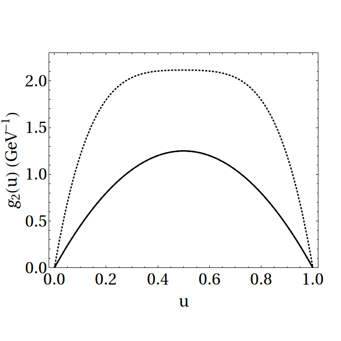
Figure 2: The functions $h_{2}(\omega)$ (left) and $g_{2}(u)$ (right) for different models of the LCDA $\phi_{2}(\omega_{1},\omega_{2})$. Solid lines correspond to the model (158), dashed lines to (165) and light-dotted lines to Ball:2008fw (in the right figure the dashed line is on top of the solid line).

3.2.2 The Chiral-Even Projector $M^{(1)}$

For the chiral-even projector $M^{(1)}$, we again consider the convolution with a hard-scattering kernel, and obtain

$$\int\widetilde{dk_{1}}\,\int\widetilde{dk_{2}}\,{\rm tr}\left[\left(T_{0}(\omega_{1},\omega_{2})+k_{i\perp}^{\mu}T_{\mu}^{i}(\omega_{1},\omega_{2})\right)M^{(1)}(v,k_{1},k_{2})\right]$$ (178)

$$= \int d\omega_{1}\,d\omega_{2}\,\int\limits_{\omega_{1}}^{\infty}dx_{1}\int\limits_{\omega_{2}}^{\infty}dx_{2}\Bigg{\{}$$ (179)

$$\quad\,{\rm tr}\left[T_{0}(\omega_{1},\omega_{2})\left(\omega_{2}\,(x_{1}-\omega_{1})\,\frac{\hbox to0.0pt{\hbox to6.00235pt{\hfil/\hfil}\hss}n_{+}\hbox to0.0pt{\hbox to6.00235pt{\hfil/\hfil}\hss}n_{-}}{4}+\omega_{1}\,(x_{2}-\omega_{2})\,\frac{\hbox to0.0pt{\hbox to6.00235pt{\hfil/\hfil}\hss}n_{-}\hbox to0.0pt{\hbox to6.00235pt{\hfil/\hfil}\hss}n_{+}}{4}\right)\right]$$ (180)

$$-{\rm tr}\left[T_{\mu}^{1}(\omega_{1},\omega_{2})\left(\omega_{1}\omega_{2}\,(x_{1}-\omega_{1})\,\frac{\hbox to0.0pt{\hbox to6.00235pt{\hfil/\hfil}\hss}n_{+}}{2}+\omega_{1}\,(x_{1}-\omega_{1})\,(x_{2}-\omega_{2})\,\frac{\hbox to0.0pt{\hbox to6.00235pt{\hfil/\hfil}\hss}n_{-}}{2}\right)\frac{\gamma_{\perp}^{\mu}}{2}\right]$$ (181)

$$-{\rm tr}\left[T_{\mu}^{2}(\omega_{1},\omega_{2})\,\frac{\gamma_{\perp}^{\mu}}{2}\left(\omega_{1}\omega_{2}\,(x_{2}-\omega_{2})\,\frac{\hbox to0.0pt{\hbox to6.00235pt{\hfil/\hfil}\hss}n_{+}}{2}+\omega_{2}\,(x_{1}-\omega_{1})\,(x_{2}-\omega_{2})\,\frac{\hbox to0.0pt{\hbox to6.00235pt{\hfil/\hfil}\hss}n_{-}}{2}\right)\right]$$ (182)

$$\qquad\Bigg{\}}\,\psi_{s}(x_{1},x_{2})\,.$$ (183)

Comparison with the momentum-space expression (130) yields

$$\phi_{3}^{-+}(\omega_{1},\omega_{2})=2\left(\phi_{3}^{(0)}(\omega_{1},\omega_{2})+\phi_{3}^{(i)}(\omega_{1},\omega_{2})\right) =2\,\int\limits_{\omega_{1}}^{\infty}dx_{1}\int\limits_{\omega_{2}}^{\infty}dx_{2}\,\omega_{2}\,(x_{1}-\omega_{1})\,\psi_{s}(x_{1},x_{2})\,,$$ (184)

$$\phi_{3}^{+-}(\omega_{1},\omega_{2})=2\left(\phi_{3}^{(0)}(\omega_{1},\omega_{2})+\phi_{3}^{(ii)}(\omega_{1},\omega_{2})\right) =2\,\int\limits_{\omega_{1}}^{\infty}dx_{1}\int\limits_{\omega_{2}}^{\infty}dx_{2}\,\omega_{1}\,(x_{2}-\omega_{2})\,\psi_{s}(x_{1},x_{2})\,,$$ (185)

and

$$\phi_{3}^{(0)}(\omega_{1},\omega_{2}) =\int\limits_{\omega_{1}}^{\infty}dx_{1}\int\limits_{\omega_{2}}^{\infty}dx_{2}\,\omega_{1}\omega_{2}\,\psi_{s}(x_{1},x_{2})\,,$$ (186)

$$\phi_{Y}(\omega_{1},\omega_{2}) =\frac{1}{2}\,\int\limits_{\omega_{1}}^{\infty}dx_{1}\int\limits_{\omega_{2}}^{\infty}dx_{2}\,(2\omega_{1}-x_{1})\,(2\omega_{2}-x_{2})\,\psi_{s}(x_{1},x_{2})\,.$$ (187)

Again, the wave function $\psi_{s}$ in our approximation can be reconstructed from

$$\psi_{s}(x_{1},x_{2}) =\frac{d^{2}}{dx_{1}\,dx_{2}}\left(\frac{\phi_{3}^{(0)}(x_{1},x_{2})}{x_{1}x_{2}}\right)\qquad\quad\mbox{(WW)}\,.$$ (188)

With the exponential model for the wave function, we now obtain

$$\psi_{s}(x_{1},x_{2}) \to\frac{\exp\left(-\frac{x_{1}+x_{2}}{\omega_{0}}\right)}{\omega_{0}^{6}}\,,$$ (189)

which yields

$$\phi_{3}^{-+}(\omega_{1},\omega_{2}) \to\frac{2\,\omega_{2}}{\omega_{0}^{3}}\,e^{-(\omega_{1}+\omega_{2})/\omega_{0}}\,,\qquad\phi_{3}^{+-}(\omega_{1},\omega_{2})\to\frac{2\,\omega_{1}}{\omega_{0}^{3}}\,e^{-(\omega_{1}+\omega_{2})/\omega_{0}}\,,$$ (190)

and

$$\phi_{3}^{(0)}(\omega_{1},\omega_{2}) \to\frac{\omega_{1}\omega_{2}}{\omega_{0}^{4}}\,e^{-(\omega_{1}+\omega_{2})/\omega_{0}}\,,$$ (191)

$$\phi_{Y}(\omega_{1},\omega_{2}) \to\frac{(\omega_{1}-\omega_{0})(\omega_{2}-\omega_{0})}{2\omega_{0}^{4}}\,e^{-(\omega_{1}+\omega_{2})/\omega_{0}}\,.$$ (192)

The free parton picture now yields

$$\phi_{3}^{-+}(\omega_{1},\omega_{2}) \to\frac{15\,\omega_{2}\,(2\bar{\Lambda}-\omega_{1}-\omega_{2})^{2}}{4\,\bar{\Lambda}^{5}}\,\theta(2\bar{\Lambda}-\omega_{1}-\omega_{2})\,,$$ (193)

$$\phi_{3}^{+-}(\omega_{1},\omega_{2}) \to\frac{15\,\omega_{1}\,(2\bar{\Lambda}-\omega_{1}-\omega_{2})^{2}}{4\,\bar{\Lambda}^{5}}\,\theta(2\bar{\Lambda}-\omega_{1}-\omega_{2})\,,$$ (194)

etc.

3.3 Renormalization-Group Evolution

In the following, we will focus on the twist-2 $\Lambda_{b}$ LCDA $\phi_{2}(\omega_{1},\omega_{2})$ which enters the leading terms in factorization theorems for exclusive heavy-to-light decay amplitudes in the heavy-quark limit, see e.g. Wang:2011uv . Its one-loop RG equation has been extensively discussed in Ball:2008fw , and reads

$$\frac{d\phi_{2}(\omega_{1},\omega_{2},\mu)}{d\ln\mu} =-\left[\Gamma_{\rm cusp}(\alpha_{s})\,\ln\frac{\mu}{\sqrt{\omega_{1}\omega_{2}}}+\gamma_{+}(\alpha_{s})\right]\phi_{2}(\omega_{1},\omega_{2},\mu)$$ (195)

$$\qquad-\frac{\omega_{1}}{2}\,\int_{0}^{\infty}d\eta_{1}\,\Gamma_{+}(\omega_{1},\eta_{1},\alpha_{s})\,\phi_{2}(\eta_{1},\omega_{2},\mu)$$ (196)

$$\qquad-\frac{\omega_{2}}{2}\,\int_{0}^{\infty}d\eta_{2}\,\Gamma_{+}(\omega_{2},\eta_{2},\alpha_{s})\,\phi_{2}(\omega_{1},\eta_{2},\mu)$$ (197)

$$\qquad+\frac{\alpha_{s}C_{F}}{2\pi}\,\int_{0}^{1}dv\,V^{\rm ERBL}(u,v)\,\phi_{2}(v\omega,\bar{v}\omega,\mu)\,,$$ (198)

where $\omega=\omega_{1}+\omega_{2}$, and $u=1-\bar{u}=\omega_{1}/\omega$, and $\bar{v}=1-v$. Here the first three lines correspond to the LN kernel for heavy baryons with the same anomalous dimensions as in (12), whereas the last term is the ERBL kernel Efremov:1979qk ; Lepage:1979zb , which arises from gluon exchange among the light quarks in the heavy baryon.

3.3.1 Analytic Solution

We follow a similar strategy as for the $B$-meson LCDA $\phi_{+}$, and as a first step introduce the logarithmic Fourier transform (which is in almost one-to-one correspondence to the Mellin moments discussed in Ball:2008fw ),

$$\varphi_{2}(\theta_{1},\theta_{2},\mu) =\int_{0}^{\infty}\frac{d\omega_{1}}{\omega_{1}}\,\int_{0}^{\infty}\frac{d\omega_{2}}{\omega_{2}}\,\phi_{2}(\omega_{1},\omega_{2},\mu)\left(\frac{\omega_{1}}{\mu}\right)^{-i\theta_{1}}\left(\frac{\omega_{2}}{\mu}\right)^{-i\theta_{2}}\,.$$ (199)

Next, we introduce the ansatz

$$\varphi_{2}(\theta_{1},\theta_{2},\mu) :=\frac{\Gamma(1-i\theta_{1})\,\Gamma(1-i\theta_{2})}{\Gamma(1+i\theta_{1})\,\Gamma(1+i\theta_{2})}\,\int_{0}^{\infty}\frac{d\omega_{1}^{\prime}}{\omega_{1}^{\prime}}\,\int_{0}^{\infty}\frac{d\omega_{2}^{\prime}}{\omega_{2}^{\prime}}\,\rho_{2}(\omega_{1}^{\prime},\omega_{2}^{\prime},\mu)\left(\frac{\mu}{\omega_{1}^{\prime}}\right)^{i\theta_{1}}\left(\frac{\mu}{\omega_{2}^{\prime}}\right)^{i\theta_{2}}$$ (200)

in complete analogy to the mesonic case, such that

$$\phi_{2}(\omega_{1},\omega_{2},\mu) =\int_{0}^{\infty}\frac{d\omega_{1}^{\prime}}{\omega_{1}^{\prime}}\,\int_{0}^{\infty}\frac{d\omega_{2}^{\prime}}{\omega_{2}^{\prime}}\,\sqrt{\frac{\omega_{1}\omega_{2}}{\omega_{1}^{\prime}\omega_{2}^{\prime}}}\,J_{1}\left(2\sqrt{\frac{\omega_{1}}{\omega_{1}^{\prime}}}\right)J_{1}\left(2\sqrt{\frac{\omega_{2}}{\omega_{2}^{\prime}}}\right)\rho_{2}(\omega_{1}^{\prime},\omega_{2}^{\prime},\mu)\,.$$ (201)

The inverse transformation that expresses the dual spectral function $\rho_{2}(\omega_{1}^{\prime},\omega_{2}^{\prime})$ in terms of the momentum-space LCDA is then given by

$$\rho_{2}(\omega_{1}^{\prime},\omega_{2}^{\prime},\mu)=\int_{0}^{\infty}{d\omega_{1}\over\omega_{1}}\int_{0}^{\infty}{d\omega_{2}\over\omega_{2}}\sqrt{{\omega_{1}\omega_{2}\over\omega_{1}^{\prime}\omega_{2}^{\prime}}}\,\,J_{1}\left(2\sqrt{{\omega_{1}\over\omega_{1}^{\prime}}}\right)\,J_{1}\left(2\sqrt{{\omega_{2}\over\omega_{2}^{\prime}}}\right)\,\,\phi_{2}(\omega_{1},\omega_{2},\mu)\,.$$ (202)

The one-loop RG equation (198) can be rewritten for the spectral function $\rho_{2}(\omega_{1}^{\prime},\omega_{2}^{\prime})$ in a straightforward manner. In the absence of the ERBL kernel, the LN terms alone would take an analogous factorized form as in the case of the $B$-meson spectral function $\rho_{B}^{+}(\omega^{\prime},\mu)$,

$$\frac{d\rho_{2}(\omega_{1}^{\prime},\omega_{2}^{\prime},\mu)}{d\ln\mu}\Big{|}_{\rm LN}= -\left[\Gamma_{\rm cusp}(\alpha_{s})\,\ln\frac{\mu}{\sqrt{\hat{\omega}_{1}^{\prime}\hat{\omega}_{2}^{\prime}}}+\gamma_{+}(\alpha_{s})\right]\rho_{2}(\omega_{1}^{\prime},\omega_{2}^{\prime},\mu)\,.$$ (203)

In this approximation the RG equation would simply be solved by

$$\rho_{2}(\omega_{1}^{\prime},\omega_{2}^{\prime},\mu)\Big{|}_{\rm LN} =e^{V}\left(\frac{\mu_{0}}{\sqrt{\hat{\omega}_{1}^{\prime}\hat{\omega}_{2}^{\prime}}}\right)^{-g}\rho_{2}(\omega_{1}^{\prime},\omega_{2}^{\prime},\mu_{0})\,,$$ (204)

with $\hat{\omega}^{\prime}_{i}=e^{-2\gamma_{E}}\,\omega^{\prime}_{i}$, and the RG functions $V$ and $g$ from (15). The derivation of the ERBL term for the evolution of $\rho_{2}(\omega_{1}^{\prime},\omega_{2}^{\prime},\mu)$, however, is more complicated (the details can be found in Appendix B). Interestingly, the final result takes a simple form when written in terms of the reduced dual momentum and dual momentum fractions,

$$\omega_{r}^{\prime}\equiv\frac{\omega_{1}^{\prime}\omega_{2}^{\prime}}{\omega_{1}^{\prime}+\omega_{2}^{\prime}} \qquad\mbox{and}\quad u^{\prime}=1-\bar{u}^{\prime}=\frac{\omega_{1}^{\prime}}{\omega_{1}^{\prime}+\omega_{2}^{\prime}}\,.$$ (205)

Writing

$$\rho_{2}(\omega_{1}^{\prime},\omega_{2}^{\prime})\equiv\hat{\rho}_{2}(\omega_{r}^{\prime},u^{\prime})\,$$ (206)

we obtain

$$\frac{d\hat{\rho}_{2}(\omega_{r}^{\prime},u^{\prime},\mu)}{d\ln\mu}\Big{|}_{\rm LN+ERBL}= -\left[\Gamma_{\rm cusp}(\alpha_{s})\,\ln\frac{\mu\,\sqrt{u^{\prime}\bar{u}^{\prime}}}{\hat{\omega}_{r}^{\prime}}+\gamma_{+}(\alpha_{s})\right]\hat{\rho}_{2}(\omega_{r}^{\prime},u^{\prime},\mu)$$ (207)

$$\quad+\frac{\alpha_{s}C_{F}}{2\pi}\,\int_{0}^{1}dv^{\prime}\,V^{\rm ERBL}(u^{\prime},v^{\prime})\,\hat{\rho}_{2}\left(\omega_{r}^{\prime},v^{\prime},\mu\right)\,.$$ (208)

If we expand the spectral function in terms of Gegenbauer polynomials $C_{n}^{(3/2)}(2u^{\prime}-1)$, which are the eigenfunctions of the ERBL kernel,

$$\hat{\rho}_{2}(\omega_{r}^{\prime},u^{\prime},\mu) :=\sum_{n=0,2,4,\ldots}^{\infty}u^{\prime}\,\bar{u}^{\prime}\,f_{n}(\omega_{r}^{\prime},\mu)\,C_{n}^{(3/2)}(2u^{\prime}-1)\,,$$ (209)

the coefficients $f_{n}(\omega_{r}^{\prime},\mu)$ satisfy the RG equation

$$\frac{df_{n}(\omega_{r}^{\prime},\mu)}{d\ln\mu}= -\left[\Gamma_{\rm cusp}(\alpha_{s})\,\ln\frac{\mu}{\hat{\omega}_{r}^{\prime}}+\gamma_{+}(\alpha_{s})+\frac{\alpha_{s}C_{F}}{4\pi}\,\gamma_{n}^{\rm ERBL}\right]f_{n}(\omega_{r}^{\prime},\mu)$$ (210)

$$\qquad-\Gamma_{nm}(\alpha_{s})\,f_{m}(\omega_{r}^{\prime},\mu)\,,$$ (211)

with $\gamma_{n}^{\rm ERBL}$ given in (247), and a non-diagonal contribution from the substitution of variables in the LN kernel, given by

$$\Gamma_{nm}(\alpha_{s}) =\Gamma_{\rm cusp}(\alpha_{s})\,\frac{2(2n+3)}{(n+1)(n+2)}\,\int\limits_{0}^{1}du^{\prime}\,u^{\prime}\bar{u}^{\prime}\,\ln(u^{\prime}\bar{u}^{\prime})\,C_{n}^{(3/2)}(2u^{\prime}-1)\,C_{m}^{(3/2)}(2u^{\prime}-1)$$

$$=-\Gamma_{\rm cusp}(\alpha_{s})\left(\begin{array}[]{cccc}\frac{5}{6}&\frac{3}{10}&\frac{3}{28}&\cdots\\ \frac{7}{60}&\frac{473}{420}&\frac{7}{18}&\cdots\\ \frac{11}{420}&\frac{11}{45}&\frac{16.847}{13.860}&\cdots\\ \cdots&\cdots&\cdots&\cdots\end{array}\right)\,,$$ (216)

where the different lines refer to $n=0,2,4,\text{etc}$ and the columns to $m=0,2,4,\text{etc}$. As one can see, the off-diagonal terms are typically smaller than the diagonal ones, and therefore, as a first approximation could be neglected. In that case, the particular form of the leading-twist baryon LCDA in (177), which translates into

$$\hat{\rho}_{2}(\omega_{r}^{\prime},u^{\prime},\mu) \to u^{\prime}\,\bar{u}^{\prime}\,f_{0}(\omega_{r}^{\prime},\mu)\,,$$ (217)

and

$$\phi_{2}(\omega_{1},\omega_{2},\mu) \to\frac{\omega_{1}\omega_{2}}{\omega_{1}+\omega_{2}}\,\int_{0}^{\infty}\frac{d\omega_{r}^{\prime}}{(\omega_{r}^{\prime})^{2}}\,\sqrt{\frac{\omega_{r}^{\prime}}{\omega_{1}+\omega_{2}}}\,J_{3}\left(2\,\sqrt{\frac{\omega_{1}+\omega_{2}}{\omega_{r}^{\prime}}}\right)f_{0}(\omega_{r}^{\prime},\mu)\,,$$ (218)

and

$$\psi_{v}(x_{1}+x_{2},\mu) \to\frac{1}{(x_{1}+x_{2})^{5/2}}\,\int_{0}^{\infty}d\omega_{r}^{\prime}\,\frac{1}{(\omega_{r}^{\prime})^{5/2}}\,J_{5}\left(2\,\sqrt{\frac{x_{1}+x_{2}}{\omega_{r}^{\prime}}}\right)f_{0}(\omega_{r}^{\prime},\mu)\,,$$ (219)

would be stable under evolution. Diagonalizing the r.h.s. of the RG equation, truncated to a finite number of Gegenbauer coefficients, is now also a straightforward task, which will be illustrated below. As already discussed in Ball:2008fw the numerical effect of the ERBL term is in any case expected to be sub-leading, and for practical applications it should be sufficient to treat it in an approximate way.

We finally note that the connection between the function $\tilde{\phi}_{2}(\tau_{1},\tau_{2})$, appearing in the light-cone matrix elements in coordinate space, and the spectral function $\hat{\rho}_{2}(\omega_{r}^{\prime},u^{\prime})$ in the baryonic case is given by

$$\hat{\rho}_{2}(\omega_{r}^{\prime},u^{\prime},\mu) =\int\frac{d\tau_{1}}{2\pi}\,\frac{d\tau_{2}}{2\pi}\left(1-\exp\left[-\frac{i\bar{u}^{\prime}}{\omega_{r}^{\prime}\tau_{1}}\right]\right)\left(1-\exp\left[-\frac{iu^{\prime}}{\omega_{r}^{\prime}\tau_{2}}\right]\right)\tilde{\phi}_{2}(\tau_{1},\tau_{2},\mu)\,.$$ (220)

3.3.2 Numerical Examples and Asymptotic Form

In the following, we study the coefficient functions $f_{0,2}(\omega_{r}^{\prime},\mu)$ and their RG behaviour, starting from different models for the LCDA $\phi_{2}$ defined at some input scale $\mu_{0}$. For a given LCDA, making use of (272) in the Appendix, we find (using $\omega_{1}=u\omega$, $\omega_{2}=\bar{u}\omega$)

$$f_{n}(\omega_{r}^{\prime},\mu_{0}) =\frac{4\,(2n+3)}{(n+1)(n+2)}\int\limits_{0}^{\infty}\frac{d\omega}{\omega}\sqrt{\frac{\omega}{\omega_{r}^{\prime}}}\,J_{2n+3}\left(2\sqrt{\frac{\omega}{\omega_{r}^{\prime}}}\right)\int\limits_{0}^{1}du\,C_{n}^{(3/2)}(2u-1)\,\phi_{2}(u\omega,\bar{u}\omega,\mu_{0})$$ (221)

Notice that the Gegenbauer expansion of the original LCDA $\phi_{2}(u\omega,\bar{u}\omega)$ directly translates to the Gegenbauer expansion of the spectral function $\hat{\rho}_{2}(\omega_{r}^{\prime},u^{\prime})$. For the models discussed above (169), this leads to

model 1: $$f_{0}(\omega_{r}^{\prime},\mu_{0})=\frac{1}{(\omega_{r}^{\prime})^{2}}\,e^{-\omega_{0}/\omega_{r}^{\prime}}\,,\qquad f_{n\geq 2}(\omega_{r}^{\prime},\mu_{0})=0\,;$$ (222)

model 2: $$f_{0}(\omega_{r}^{\prime},\mu_{0})=\frac{1}{(\omega_{r}^{\prime})^{2}}\,e^{-\epsilon_{0}/\omega_{r}^{\prime}}\,,\qquad f_{n>2}(\omega_{r}^{\prime},\mu_{0})=0\,,$$ (223)

$$f_{2}(\omega_{r}^{\prime},\mu_{0})={a_{2}\over(\omega_{r}^{\prime})^{2}}\bigg{\{}e^{-{1/x_{r}}}(720\,x_{r}^{5}+600\,x_{r}^{4}+240\,x_{r}^{3}+60\,x_{r}^{2}+10\,x_{r}+1)$$ (224)

$$\phantom{f_{0}(\omega_{r}^{\prime},\mu_{0})=}\qquad+120\,x_{r}^{4}\,(1-6\,x_{r})\bigg{\}}\,,\quad(x_{r}\equiv\omega_{r}^{\prime}/\epsilon_{1})\,;$$ (225)

model 3: $$f_{0}(\omega_{r}^{\prime},\mu_{0})=\frac{15}{\bar{\Lambda}^{2}}\,\sqrt{{2\omega_{r}^{\prime}\over\bar{\Lambda}}}\,J_{5}\left(2\sqrt{{2\bar{\Lambda}\over\omega_{r}^{\prime}}}\right)\,,\qquad f_{n\geq 2}(\omega_{r}^{\prime},\mu_{0})=0\,.$$ (226)

The qualitative behaviour of model 1 and model 3 is similar to what we have discussed for the corresponding functions in the $B$-meson case. Notice that the contribution of the coefficient function $f_{2}(\omega_{r}^{\prime})$ to the spectral function $\hat{\rho}_{2}(\omega_{r}^{\prime},u^{\prime})$ in model 2 is concentrated at very low values of $\omega_{r}^{\prime}$, while for generic values of $\omega_{r}^{\prime}$ its contribution is practically negligible. In order to study systematic deviations from the particular form of $\hat{\rho}_{2}(\omega_{r}^{\prime},u^{\prime})$ in (217), it would therefore be more convenient to define a modified version, for which we propose

model 2’: $$f_{0}(\omega_{r}^{\prime},\mu_{0})\equiv\frac{1}{(\omega_{r}^{\prime})^{2}}\,e^{-\epsilon_{0}/\omega_{r}^{\prime}}\,,\qquad f_{2}(\omega_{r}^{\prime},\mu_{0})\equiv\frac{a_{2}}{6}\,{\epsilon_{1}^{2}\over(\omega_{r}^{\prime})^{4}}\,e^{-\epsilon_{1}/\omega_{r}^{\prime}}\,,$$ (227)

which has the same functional form as model 2 at large $\omega_{r}^{\prime}$ (except for a different normalization) such that the $1/\omega_{r}^{\prime}$ moment of $f_{2}(\omega_{r}^{\prime})$ in model 2 and model 2’ coincide. In the original momentum space, this corresponds to a LCDA

model 2’: $$\phi_{2}(\omega_{1},\omega_{2},\mu_{0})=\frac{\omega_{1}\omega_{2}}{\epsilon_{0}^{4}}\,e^{-(\omega_{1}+\omega_{2})/\epsilon_{0}}+a_{2}\,\frac{\omega_{1}\omega_{2}\left(\omega_{1}^{2}-3\omega_{1}\omega_{2}+\omega_{2}^{2}\right)}{\epsilon_{1}^{6}}\,e^{-(\omega_{1}+\omega_{2})/\epsilon_{1}}\,.$$ (228)

Concerning the RG behaviour, we first note that the explicit solution for the functions $f_{0,2}(\omega_{r}^{\prime},\mu)$ in the absence of higher Gegenbauer coefficients reads

$$f_{0}(\omega_{r}^{\prime},\mu) =e^{V}\left({\mu_{0}\over\hat{\omega}_{r}^{\prime}}\right)^{-g}\left\{c_{1}\,e^{0.877g}-0.378\,c_{2}\,e^{0.040g}\right\}\,,$$ (229)

$$f_{2}(\omega_{r}^{\prime},\mu) =e^{V}\left({\mu_{0}\over\hat{\omega}_{r}^{\prime}}\right)^{-g}\left\{0.147\,c_{1}\,e^{0.877g}+c_{2}\,e^{0.040g}\right\}\,,$$ (230)

where the two integration constants are related to the initial condition of the evolution via

$$c_{1} =0.947\,f_{0}(\omega_{r}^{\prime},\mu_{0})+0.358\,f_{2}(\omega_{r}^{\prime},\mu_{0})\,,$$ (231)

$$c_{2} =-0.139\,f_{0}(\omega_{r}^{\prime},\mu_{0})+0.947\,f_{2}(\omega_{r}^{\prime},\mu_{0})\,.$$ (232)

In the asymptotic limit, i.e. for large renormalization scales and large values of $g$, the first exponential in the curly brackets dominates, and the ratio of the two coefficients approaches a constant, $f_{2}/f_{0}\simeq 0.147$. This is illustrated for model 2 and model 2’ in Fig. 3. For both models, the asymptotic value for $f_{2}/f_{0}$ is reached for $g\mathrel{\hbox{\hbox to0.0pt{\hbox{\lower 4.0pt\hbox{$\sim$}}\hss}\hbox{$>$}}}3$.

When higher Gegenbauer moments are included, the asymptotic form is similarly determined by the largest eigenvalue of the RG equation (211) after subtracting the LN terms. We then find that the ratio $f_{2}/f_{0}$ converges to about 20%, and that the admixtures of the higher Gegenbauer moments are less important, with $f_{4}/f_{0}\simeq 9\%$, $f_{6}/f_{0}\simeq 5\%$, etc. The resulting asymptotic $u^{\prime}$-dependence of the spectral function, corresponding to the different levels of truncation in the Gegenbauer expansion, is illustrated in Fig. 4. The functional form that is approached asymptotically is well approximated by $\hat{\rho}_{2}(\omega_{r}^{\prime},u^{\prime},\mu)\propto(u^{\prime}(1-u^{\prime}))^{1/3}f_{0}(\omega_{r}^{\prime},\mu)$.

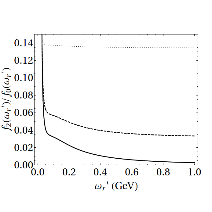
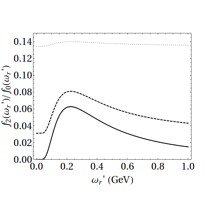
Figure 3: Numerical examples for the evolution of the ratio of Gegenbauer coefficient functions $f_{2}(\omega_{r}^{\prime},\mu)/f_{0}(\omega_{r}^{\prime},\mu)$. Left: for model 2 from Ball:2008fw . Right: for model 2’, with $a_{2}=1/3$, $\epsilon_{0}=0.2$ GeV, $\epsilon_{1}=0.65$ GeV, see text. Solid lines: input model at $\mu_{0}$; dashed lines: RG evolution corresponding to $g=0.3$; dotted line: with $g=3$.

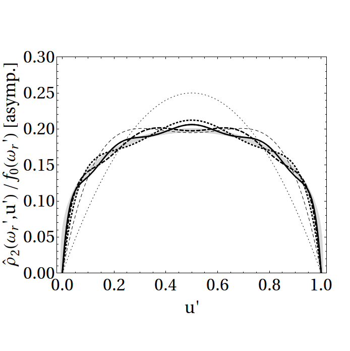
Figure 4: Asymptotic $u^{\prime}$-dependence of the spectral function $\hat{\rho}_{2}(\omega_{r}^{\prime},u^{\prime},\mu)/f_{0}(\omega_{r}^{\prime},\mu)$, for different levels of truncation in the Gegenbauer expansion: $n=0$ (thin dotted), $n=2$ (thin dashed), $n=4$ (thick dotted), $n=6$ (thick dashed), $n=8$ (solid). The gray band shows the approximation $\hat{\rho}_{2}(\omega_{r}^{\prime},u^{\prime},\mu)/f_{0}(\omega_{r}^{\prime},\mu)\propto(u^{\prime}(1-u^{\prime}))^{1/3}$.

4 Summary

We have investigated light-cone distribution amplitudes (LCDAs) as defined in heavy-quark effective theory for $B$-mesons and $\Lambda_{b}$-baryons. On the one hand, we have constructed easy-to-use momentum-space representations for the leading Fock states, which reduce to an expansion in terms of conventional LCDAs when convoluted with a hard-scattering kernel in the (collinear) QCD factorization approach, but also allows for a comparison with models for transverse-momentum-dependent wave functions. In the simplest case, our construction automatically implements so-called Wandzura-Wilczek relations, which connect different LCDAs in the limit where higher Fock-state contributions to the equations of motion are neglected. We have also illustrated how corrections to the Wandzura-Wilczek approximation can be taken into account consistently within our approach. For the baryonic case in particular, our ansatz leads to a significant reduction of independent hadronic functions which appear at sub-leading order in the collinear expansion. The sub-leading functions are needed, for instance, in SCET sum rules analyses of exclusive $\Lambda_{b}$ transitions for cases where the standard QCD factorization approach would lead to endpoint-sensitive (formally ill-defined) convolution integrals (see e.g. the discussion in Feldmann:2011xf ).

Furthermore, we have found a new representation of LCDAs in terms of dual spectral functions, which are the eigenfunctions of the Lange-Neubert renormalization kernel. The connection between the LCDAs and their dual representations is via convolution integrals with Bessel functions. In the dual space, the solutions to the renormalization-group equations are extremely simple. In the mesonic case, they are local in the dual momentum variable $\omega^{\prime}$ of the light quark. We have demonstrated the simplifications that arise when re-formulating the factorization theorem for radiative leptonic $B\to\gamma\ell\nu$ decays in terms of the new spectral function and an associated new hard-collinear function, which evolve both by a multiplicative factor. Again, the baryonic case is more complicated, because the Lange-Neubert kernel and the Efremov-Radyushkin–Brodsky-Lepage kernel cannot be separated in the usual momentum space. In the dual space, however, a separation of the reduced dual momentum $\omega_{r}^{\prime}=\omega_{1}^{\prime}\omega_{2}^{\prime}/(\omega_{1}^{\prime}+\omega_{2}^{\prime})$ and the dual momentum fraction $u^{\prime}=\omega_{1}^{\prime}/(\omega_{1}^{\prime}+\omega_{2}^{\prime})$ is possible, which opens the way for a systematic solution of the baryonic renormalization-group equation in terms of an expansion in Gegenbauer polynomials (as known from the pion LCDAs).

In summary, our results should be helpful in calculations of exclusive decay amplitudes for hadrons containing a heavy quark in the framework of QCD factorization, soft-collinear effective theory or light-cone sum rules. Specifically for applications involving heavy baryons, we expect more transparent and efficient estimates of theoretical hadronic uncertainties, which are needed, for instance, to constrain physics beyond the Standard Model from rare decays like $\Lambda_{b}\to\Lambda\mu^{+}\mu^{-}$ which are currently studied at hadron colliders.

Appendix A $B$-Meson Projectors in arbitrary Frame

In certain applications, one would need the momentum-space projectors in an arbitrary frame, where $n_{-}\cdot n_{+}=2$, but the heavy-quark velocity reads

$$v^{\mu}=(n_{-}v)\,\frac{n_{+}^{\mu}}{2}+(n_{+}v)\,\frac{n_{-}^{\mu}}{2}+v_{\perp}^{\mu}\,,\qquad v_{\perp}^{2}=1-(n_{-}v)(n_{+}v)\,.$$

A.1 2-Particle Projector

Taking $(n_{-}z)\ll z_{\perp}\ll(n_{+}z)$ and expanding the non-local matrix element for the $B$-meson 2-particle LCDAs, we then obtain

$$2\,\tilde{\Phi}_{B}^{+}(t,z^{2})+\frac{\tilde{\Phi}_{B}^{-}(t,z^{2})-\tilde{\Phi}_{B}^{+}(t,z^{2})}{t}\,\not{z}$$ (233)

$$\qquad=2\,\tilde{\phi}_{B}^{+}(\tau)+\left(\tilde{\phi}_{B}^{-}(\tau)-\tilde{\phi}_{B}^{+}(\tau)\right)\frac{\not{n}_{-}}{(n_{-}v)}+\frac{\tilde{\phi}_{B}^{-}(\tau)-\tilde{\phi}_{B}^{+}(\tau)}{\tau}\,\not{z}_{\perp}$$ (234)

$$\qquad\quad+\frac{\partial}{\partial\tau}\left(2\tilde{\phi}_{B}^{+}(\tau)+\left(\tilde{\phi}_{B}^{-}(\tau)-\tilde{\phi}_{B}^{+}(\tau)\right)\frac{\not{n}_{-}}{(n_{-}v)}\right)(v_{\perp}\cdot z_{\perp})+{\cal O}(z_{\perp}^{2},n_{-}z)\,,$$ (235)

where now $\tau=\frac{(n_{-}v)\,(n_{+}z)}{2}$ can be interpreted as the Fourier-conjugated variable to the momentum component of the light anti-quark,

$$\omega=\frac{(n_{-}k)}{(n_{-}v)}\,,\qquad\omega\,\tau=\frac{(n_{-}k)(n_{+}z)}{2}\,.$$

The light-cone expansion in (235) corresponds to the momentum-space projector

$$2\phi_{B}^{+}(\omega)+\Big{(}\phi_{B}^{-}(\omega)-\phi_{B}^{+}(\omega)\Big{)}\frac{\not{n}_{-}}{(n_{-}v)}-\int_{0}^{\omega}d\eta\,\Big{(}\phi_{B}^{-}(\eta)-\phi_{B}^{+}(\eta)\Big{)}\,\gamma^{\mu}_{\perp}\,\frac{\partial}{\partial k_{\perp}^{\mu}}$$ (236)

$$\qquad{}+\omega\bigg{(}2\phi_{B}^{+}(\omega)+\Big{(}\phi_{B}^{-}(\omega)-\phi_{B}^{+}(\omega)\Big{)}\frac{\not{n}_{-}}{(n_{-}v)}\bigg{)}\left(v_{\perp}\cdot\frac{\partial}{\partial k_{\perp}}\right)$$ (237)

to be used in factorization theorems with hard-scattering kernels where the $k_{\perp}^{2}$ and $(n_{+}k)$-dependence can be neglected. Notice that the so-defined projector is manifestly invariant under Lorentz boosts, $n_{\pm}\to\gamma^{\pm 1}n_{\pm}$.

A.2 3-Particle Projector

Following the same procedure as for the 2-particle momentum-space projector, we obtain the leading contribution to the 3-particle projector in a general frame as

$${\cal M}_{B}^{(3)}{}^{\mu}(v,\omega,\xi) =-{i\over\xi}{\tilde{f}_{B}m_{B}\over 2}\,\Bigg{[}{1+\not{v}\over 2}\Bigg{\{}$$ (239)

$$\quad\left(\frac{(n_{+}v)\,n_{-}^{\mu}\not{n}_{-}-n_{-}^{\mu}+(v_{\perp}^{\mu}\not{n}_{-}+n_{-}^{\mu}\not{v}_{\perp})}{(n_{-}v)}-\gamma_{\perp}^{\mu}\right)\big{(}\Psi_{A}(\omega,\xi)-\Psi_{V}(\omega,\xi)\big{)}$$ (240)

$$\quad+\left(\frac{n_{-}^{\mu}\not{n}_{-}+n_{-}^{\mu}\not{n}_{-}\not{v}_{\perp}}{(n_{-}v)}-n_{-}^{\mu}+\gamma_{\perp}^{\mu}\not{n}_{-}\right)\frac{\Psi_{V}(\omega,\xi)}{(n_{-}v)}$$ (241)

$$\quad-\frac{n_{-}^{\mu}}{(n_{-}v)}\,X_{A}(\omega,\xi)+\frac{n_{-}^{\mu}\not{n}_{-}}{(n_{-}v)^{2}}\,Y_{A}(\omega,\xi)\Bigg{\}}\gamma_{5}\Bigg{]}\,,$$ (242)

which is again manifestly invariant under longitudinal Lorentz boosts.

Appendix B The ERBL Term for the dual LCDA of the $\Lambda_{b}$–Baryon

The ERBL contribution to the RG equation for the LCDAs $\phi_{2}(\omega_{1},\omega_{2})$ reads Ball:2008fw

$$\frac{d}{d\ln\mu}\,\phi_{2}(u\omega,\bar{u}\omega,\mu)\Big{|}_{\rm ERBL} =\frac{\alpha_{s}C_{F}}{2\pi}\,\int_{0}^{1}dv\,V^{\rm ERBL}(u,v)\,\phi_{2}(v\omega,\bar{v}\omega,\mu)\,,$$ (243)

with

$$\omega=\omega_{1}+\omega_{2}\,,\quad u=\frac{\omega_{1}}{\omega_{1}+\omega_{2}}\,,\quad\bar{u}=1-u=\frac{\omega_{2}}{\omega_{1}+\omega_{2}}\,.$$ (244)

The one-loop expression for the ERBL kernel is given by

$$V^{\rm ERBL}(u,v) =\left[\frac{1-u}{1-v}\left(1+\frac{1}{u-v}\right)\theta(u-v)+\frac{u}{v}\left(1+\frac{1}{v-u}\right)\theta(v-u)\right]_{+}$$ (245)

$$=-u(1-u)\sum_{n=0}^{\infty}\frac{2(2n+3)}{(n+1)(n+2)}\,\gamma_{n}^{\rm ERBL}\,C_{n}^{3/2}(2u-1)\,C_{n}^{3/2}(2v-1)\,,$$ (246)

where in the last line we have quoted the expansion in terms of Gegenbauer polynomials Braun:2003rp , with the eigenvalues of the corresponding anomalous-dimension matrix given by

$$\gamma_{n}^{\rm ERBL} =1-\frac{2}{(n+1)(n+2)}+4\,\sum_{m=2}^{n+1}\frac{1}{m}\,.$$ (247)

The transformation to the spectral function $\rho_{2}$ reads

$$\frac{d}{d\ln\mu}\,\rho_{2}(\omega_{1}^{\prime},\omega_{2}^{\prime},\mu)\Big{|}_{\rm ERBL}$$ (248)

$$\quad=\frac{d}{d\ln\mu}\int\limits_{0}^{\infty}\frac{d\omega_{1}}{\omega_{1}}\int\limits_{0}^{\infty}\frac{d\omega_{2}}{\omega_{2}}\,\sqrt{\frac{\omega_{1}\omega_{2}}{\omega_{1}^{\prime}\omega_{2}^{\prime}}}\,J_{1}\left(2\sqrt{\frac{\omega_{1}}{\omega_{1}^{\prime}}}\right)J_{1}\left(2\sqrt{\frac{\omega_{2}}{\omega_{2}^{\prime}}}\right)\phi_{2}(\omega_{1},\omega_{2},\mu)\Big{|}_{\rm ERBL}$$ (249)

$$\quad=\frac{d}{d\ln\mu}\int\limits_{0}^{\infty}\frac{d\omega}{\omega}\int\limits_{0}^{1}\frac{du}{u\bar{u}}\,\sqrt{\frac{u\bar{u}\omega^{2}}{\omega_{1}^{\prime}\omega_{2}^{\prime}}}\,J_{1}\left(2\sqrt{\frac{u\omega}{\omega_{1}^{\prime}}}\right)J_{1}\left(2\sqrt{\frac{\bar{u}\omega}{\omega_{2}^{\prime}}}\right)\phi_{2}(u\omega,\bar{u}\omega,\mu)\Big{|}_{\rm ERBL}$$ (250)

$$\quad=\frac{\alpha_{s}C_{F}}{2\pi}\,\int\limits_{0}^{\infty}\frac{d\omega}{\omega}\int\limits_{0}^{1}\frac{du}{u\bar{u}}\,\sqrt{\frac{u\bar{u}\omega^{2}}{\omega_{1}^{\prime}\omega_{2}^{\prime}}}\,J_{1}\left(2\sqrt{\frac{u\omega}{\omega_{1}^{\prime}}}\right)J_{1}\left(2\sqrt{\frac{\bar{u}\omega}{\omega_{2}^{\prime}}}\right)$$ (251)

$$\qquad\ \times\int_{0}^{1}dv\,V^{\rm ERBL}(u,v)\,\phi_{2}(v\omega,\bar{v}\omega,\mu)$$ (252)

$$\quad=\frac{\alpha_{s}C_{F}}{2\pi}\,\int\limits_{0}^{\infty}\frac{d\omega}{\omega}\int\limits_{0}^{1}\frac{du}{u\bar{u}}\,\sqrt{\frac{u\bar{u}\omega^{2}}{\omega_{1}^{\prime}\omega_{2}^{\prime}}}\,J_{1}\left(2\sqrt{\frac{u\omega}{\omega_{1}^{\prime}}}\right)J_{1}\left(2\sqrt{\frac{\bar{u}\omega}{\omega_{2}^{\prime}}}\right)\int_{0}^{1}dv\,V^{\rm ERBL}(u,v)$$ (253)

$$\qquad\ \times\int\limits_{0}^{\infty}\frac{d\eta_{1}^{\prime}}{\eta_{1}^{\prime}}\int\limits_{0}^{\infty}\frac{d\eta_{2}^{\prime}}{\eta_{2}^{\prime}}\,\sqrt{\frac{v\bar{v}\omega^{2}}{\eta_{1}^{\prime}\eta_{2}^{\prime}}}\,J_{1}\left(2\sqrt{\frac{v\omega}{\eta_{1}^{\prime}}}\right)J_{1}\left(2\sqrt{\frac{\bar{v}\omega}{\eta_{2}^{\prime}}}\right)\rho_{2}(\eta_{1}^{\prime},\eta_{2}^{\prime},\mu)\,.$$ (254)

In terms of the integrals $I_{n}$ defined in (267) below, using the Gegenbauer expansion of the ERBL kernel, we can write

$$\frac{d}{d\ln\mu}\,\rho_{2}(\omega_{1}^{\prime},\omega_{2}^{\prime},\mu)\Big{|}_{\rm ERBL}$$ (255)

$$\quad=-\frac{\alpha_{s}C_{F}}{2\pi}\,\sum_{n=0}^{\infty}\frac{2(2n+3)}{(n+1)(n+2)}\,\gamma_{n}^{\rm ERBL}\int\limits_{0}^{\infty}\frac{d\omega}{\omega}\int\limits_{0}^{\infty}\frac{d\eta_{1}^{\prime}}{\eta_{1}^{\prime}}\int\limits_{0}^{\infty}\frac{d\eta_{2}^{\prime}}{\eta_{2}^{\prime}}\,$$ (256)

$$\quad\times\,\sqrt{\frac{\omega^{2}}{\omega_{1}^{\prime}\omega_{2}^{\prime}}}\,\sqrt{\frac{\omega^{2}}{\eta_{1}^{\prime}\eta_{2}^{\prime}}}\,I_{n}\left(2\sqrt{\frac{\omega}{\omega_{1}^{\prime}}},2\sqrt{\frac{\omega}{\omega_{2}^{\prime}}}\right)\,I_{n}\left(2\sqrt{\frac{\omega}{\eta_{1}^{\prime}}},2\sqrt{\frac{\omega}{\eta_{2}^{\prime}}}\right)\rho_{2}(\eta_{1}^{\prime},\eta_{2}^{\prime},\mu)\,.$$ (257)

As the integrals $I_{n}$ themselves are proportional to Bessel functions and have a homogeneous scaling with the variable $\omega$, we can use the completeness relation (266) to perform the $\omega$ integration explicitly for each individual order in the Gegenbauer expansion. It is furthermore convenient to introduce new variables

$$\omega_{r}^{\prime}\equiv\frac{\omega_{1}^{\prime}\omega_{2}^{\prime}}{\omega_{1}^{\prime}+\omega_{2}^{\prime}} \qquad\mbox{and}\quad u^{\prime}=1-\bar{u}^{\prime}=\frac{\omega_{1}^{\prime}}{\omega_{1}^{\prime}+\omega_{2}^{\prime}}\,,$$ (258)

$$\eta_{r}^{\prime}\equiv\frac{\eta_{1}^{\prime}\eta_{2}^{\prime}}{\eta_{1}^{\prime}+\eta_{2}^{\prime}} \qquad\mbox{and}\quad v^{\prime}=1-\bar{v}^{\prime}=\frac{\eta_{1}^{\prime}}{\eta_{1}^{\prime}+\eta_{2}^{\prime}}\,,$$ (259)

and to denote the spectral function in terms of the new variables according to

$$\rho_{2}(\omega_{1}^{\prime},\omega_{2}^{\prime})\equiv\hat{\rho}_{2}(\omega_{r}^{\prime},u^{\prime})\,.$$ (260)

We then obtain

$$\frac{d}{d\ln\mu}\,\hat{\rho}_{2}(\omega_{r}^{\prime},u^{\prime},\mu)\Big{|}_{\rm ERBL}$$ (261)

$$\qquad=-\frac{\alpha_{s}C_{F}}{2\pi}\,\sum_{n=0}^{\infty}\frac{2(2n+3)}{(n+1)(n+2)}\,\gamma_{n}^{\rm ERBL}\,u^{\prime}\bar{u}^{\prime}\,C_{n}^{(3/2)}(2u^{\prime}-1)$$ (262)

$$\qquad\qquad\times\int_{0}^{1}dv^{\prime}\,C_{n}^{(3/2)}(2v^{\prime}-1)\,\int_{0}^{\infty}d\eta_{r}^{\prime}\,\delta(\omega_{r}^{\prime}-\eta_{r}^{\prime})\,\hat{\rho}_{2}(\eta_{r}^{\prime},v^{\prime},\mu)$$ (263)

$$\qquad=\frac{\alpha_{s}C_{F}}{2\pi}\,\int_{0}^{1}dv^{\prime}\,V^{\rm ERBL}(u^{\prime},v^{\prime})\,\hat{\rho}_{2}(\omega_{r}^{\prime},v^{\prime},\mu)\,.$$ (264)

Appendix C Some Relations with Bessel Functions

The completeness relation for Bessel functions,

$$\int_{0}^{\infty}dz\,z\,J_{n}(az)\,J_{n}(bz) =\frac{1}{a}\,\delta(a-b)\,,$$

can be written as

$$\int_{0}^{\infty}\frac{d\omega^{\prime}}{\omega^{\prime}}\,\frac{1}{\omega^{\prime}}\,J_{n}\left(2\,\sqrt{\frac{a}{\omega^{\prime}}}\right)J_{n}\left(2\,\sqrt{\frac{b}{\omega^{\prime}}}\right)$$ (265)

$$= \int_{0}^{\infty}d\omega\,J_{n}\left(2\,\sqrt{a\omega}\right)J_{n}\left(2\,\sqrt{b\omega}\right)=\delta(a-b)\,,$$ (266)

which has been frequently used in the text.

We further define integrals with Bessel functions and Gegenbauer polynomials,

$$I_{n}(\alpha,\beta) \equiv\int_{0}^{1}dv\,\sqrt{v(1-v)}\,J_{1}(\alpha\sqrt{v})\,J_{1}(\beta\sqrt{1-v})\,C_{n}^{3/2}(2v-1)\,.$$ (267)

For the first few (even) values of $n$, we obtain

$$I_{0}(\alpha,\beta) =2\,\alpha\beta\frac{1}{(\alpha^{2}+\beta^{2})^{3/2}}\,J_{3}(\sqrt{\alpha^{2}+\beta^{2}})\,,$$ (268)

$$I_{2}(\alpha,\beta) =12\,\alpha\beta\,\frac{\alpha^{4}-3\,\alpha^{2}\beta^{2}+\beta^{4}}{(\alpha^{2}+\beta^{2})^{7/2}}\,J_{7}(\sqrt{\alpha^{2}+\beta^{2}})\,,$$ (269)

$$I_{4}(\alpha,\beta) =30\,\alpha\beta\,\frac{\alpha^{8}-10\,\alpha^{6}\beta^{2}+20\,\alpha^{4}\beta^{4}-10\,\alpha^{2}\beta^{6}+\beta^{8}}{(\alpha^{2}+\beta^{2})^{11/2}}\,J_{11}(\sqrt{\alpha^{2}+\beta^{2}})\,.$$ (270)

The general formula can be constructed by introducing the variables

$$\alpha=2\,\sqrt{\frac{x}{1-u}}\,,\quad\beta=2\,\sqrt{\frac{x}{u}}\,,\quad\Leftrightarrow\quad x=\frac{\alpha^{2}\beta^{2}}{4\,(\alpha^{2}+\beta^{2})}\,,\qquad u=\frac{\alpha^{2}}{\alpha^{2}+\beta^{2}}\,,$$ (271)

for which we obtain the compact expression

$$I_{n}(\alpha,\beta) =\frac{u(1-u)}{\sqrt{x}}\,C_{n}^{(3/2)}(2u-1)\,J_{2n+3}\left(2\sqrt{\frac{x}{u(1-u)}}\right)\,.$$ (272)

We also often used the relation

$$J_{n}(x) =\frac{x}{2n}\left(J_{n-1}(x)+J_{n+1}(x)\right)\qquad(n\geq 1)\,.$$ (273)

References

• (1) A. V. Efremov and A. V. Radyushkin, “Factorization and Asymptotical Behavior of Pion Form-Factor in QCD,” Phys. Lett. B 94 (1980) 245.
• (2) G. P. Lepage and S. J. Brodsky, “Exclusive Processes in Quantum Chromodynamics: Evolution Equations for Hadronic Wave Functions and the Form-Factors of Mesons,” Phys. Lett. B 87 (1979) 359; “Exclusive Processes in Perturbative Quantum Chromodynamics,” Phys. Rev. D 22 (1980) 2157.
• (3) A. Duncan and A. H. Mueller, “Asymptotic Behavior of Composite Particle Form-Factors and the Renormalization Group,” Phys. Rev. D 21 (1980) 1636.
• (4) V. L. Chernyak and A. R. Zhitnitsky, “Asymptotic Behavior of Exclusive Processes in QCD,” Phys. Rept.  112 (1984) 173.
• (5) G. P. Korchemsky, D. Pirjol and T. -M. Yan, “Radiative leptonic decays of $B$ mesons in QCD,” Phys. Rev. D 61 (2000) 114510 [hep-ph/9911427].
• (6) S. Descotes-Genon and C. T. Sachrajda, “Factorization, the light cone distribution amplitude of the $B$-meson and the radiative decay $B\to\gamma\ell\nu_{\ell}$,” Nucl. Phys. B 650 (2003) 356 [hep-ph/0209216].
• (7) E. Lunghi, D. Pirjol and D. Wyler, “Factorization in leptonic radiative $b\to\gamma e\nu$ decays,” Nucl. Phys. B 649 (2003) 349 [hep-ph/0210091].
• (8) S. W. Bosch, R. J. Hill, B. O. Lange and M. Neubert, “Factorization and Sudakov resummation in leptonic radiative $B$ decay,” Phys. Rev. D 67 (2003) 094014 [hep-ph/0301123].
• (9) M. Beneke and J. Rohrwild, “$B$-meson distribution amplitude from $B\to\gamma\ell\nu$,” Eur. Phys. J. C 71 (2011) 1818 [arXiv:1110.3228 [hep-ph]].
• (10) V. M. Braun and A. Khodjamirian, “Soft contribution to $B\to\gamma\ell\nu_{\ell}$ and the $B$-meson distribution amplitude,” Phys. Lett. B 718 (2013) 1014 [arXiv:1210.4453 [hep-ph]].
• (11) “QCD factorization for $B\to\pi\pi$ decays: Strong phases and CP violation in the heavy quark limit,” Phys. Rev. Lett.  83 (1999) 1914 [hep-ph/9905312]; M. Beneke, G. Buchalla, M. Neubert and C. T. Sachrajda, “QCD factorization in $B\to\pi K,\pi\pi$ decays and extraction of Wolfenstein parameters,” Nucl. Phys. B 606 (2001) 245 [hep-ph/0104110].
• (12) M. Beneke, Th. Feldmann, “Symmetry breaking corrections to heavy-to-light $B$-meson form factors at large recoil,” Nucl. Phys.  B592, 3-34 (2001) [hep-ph/0008255].
• (13) S. W. Bosch and G. Buchalla, “The Radiative decays $B\to V\gamma$ at next-to-leading order in QCD,” Nucl. Phys. B 621 (2002) 459 [hep-ph/0106081].
• (14) A. Ali and A. Y. Parkhomenko, “Branching ratios for $B\to K^{*}\gamma$ and $B\to\rho\gamma$ decays in next-to-leading order in the large energy effective theory,” Eur. Phys. J. C 23 (2002) 89 [hep-ph/0105302]; A. Ali, B. D. Pecjak and C. Greub, “$B\to V\gamma$ Decays at NNLO in SCET,” Eur. Phys. J. C 55 (2008) 577 [arXiv:0709.4422 [hep-ph]].
• (15) M. Beneke, Th. Feldmann and D. Seidel, “Systematic approach to exclusive $B\to V\ell^{+}\ell^{-}$, $V\gamma$ decays,” Nucl. Phys. B 612 (2001) 25 [hep-ph/0106067]; “Exclusive radiative and electroweak $b\to d$ and $b\to s$ penguin decays at NLO,” Eur. Phys. J. C 41 (2005) 173 [hep-ph/0412400].
• (16) A. L. Kagan and M. Neubert, “Isospin breaking in $B\to K^{*}\gamma$ decays,” Phys. Lett. B 539 (2002) 227 [hep-ph/0110078].
• (17) C. W. Bauer, S. Fleming, D. Pirjol and I. W. Stewart, “An Effective field theory for collinear and soft gluons: Heavy to light decays,” Phys. Rev. D 63 (2001) 114020 [hep-ph/0011336]; C. W. Bauer, D. Pirjol and I. W. Stewart, “Soft collinear factorization in effective field theory,” Phys. Rev. D 65 (2002) 054022 [hep-ph/0109045].
• (18) M. Beneke, A. P. Chapovsky, M. Diehl, Th. Feldmann, “Soft collinear effective theory and heavy to light currents beyond leading power,” Nucl. Phys.  B643 (2002) 431-476 [hep-ph/0206152]; M. Beneke and Th. Feldmann, “Multipole expanded soft collinear effective theory with non-Abelian gauge symmetry,” Phys. Lett. B 553 (2003) 267 [hep-ph/0211358].
• (19) F. De Fazio, Th. Feldmann, T. Hurth, “Light-cone sum rules in soft-collinear effective theory,” Nucl. Phys.  B733 (2006) 1-30 [hep-ph/0504088]; “SCET sum rules for $B\to P$ and $B\to V$ transition form factors,” JHEP 0802 (2008) 031 [arXiv:0711.3999 [hep-ph]].
• (20) A. Khodjamirian, T. Mannel and N. Offen, “$B$-meson distribution amplitude from the $B\to\pi$ form-factor,” Phys. Lett. B 620 (2005) 52 [hep-ph/0504091]; “Form-factors from light-cone sum rules with $B$-meson distribution amplitudes,” Phys. Rev.  D75 (2007) 054013. [hep-ph/0611193].
• (21) Y. Y. Keum, H. -N. Li and A. I. Sanda, “Penguin enhancement and $B\to K\pi$ decays in perturbative QCD,” Phys. Rev. D 63 (2001) 054008 [hep-ph/0004173].
• (22) C. -D. Lu, K. Ukai and M. -Z. Yang, “Branching ratio and CP violation of $B\to\pi\pi$ decays in perturbative QCD approach,” Phys. Rev. D 63 (2001) 074009 [hep-ph/0004213].
• (23) X. -G. He, T. Li, X. -Q. Li and Y. -M. Wang, “PQCD calculation for $\Lambda_{b}\to\Lambda\gamma$ in the standard model,” Phys. Rev. D 74 (2006) 034026 [hep-ph/0606025]; C. -D. Lu, Y. -M. Wang, H. Zou, A. Ali and G. Kramer, “Anatomy of the pQCD Approach to the Baryonic Decays $\Lambda_{b}\to p\pi,pK$,” Phys. Rev. D 80 (2009) 034011 [arXiv:0906.1479 [hep-ph]].
• (24) A. G. Grozin and M. Neubert, “Asymptotics of heavy-meson form factors,” Phys. Rev.  D 55 (1997) 272 [arXiv:hep-ph/9607366]; A. G. Grozin, “$B$-meson distribution amplitudes,” Int. J. Mod. Phys.  A 20 (2005) 7451 [arXiv:hep-ph/0506226].
• (25) H. Kawamura, J. Kodaira, C. -F. Qiao, K. Tanaka, “$B$ meson light cone distribution amplitudes in the heavy quark limit,” Phys. Lett. B 523 (2001) 111 [Erratum-ibid. B 536 (2002) 344] [hep-ph/0109181].
• (26) P. Ball, V. M. Braun and E. Gardi, “Distribution Amplitudes of the $\Lambda_{b}$ Baryon in QCD,” Phys. Lett. B 665 (2008) 197 [arXiv:0804.2424 [hep-ph]].
• (27) Th. Feldmann and M. W. Y. Yip, “Form Factors for $\Lambda_{b}\to\Lambda$ Transitions in SCET,” Phys. Rev. D 85 (2012) 014035 [Erratum-ibid. D 86 (2012) 079901] [arXiv:1111.1844 [hep-ph]]; M. W. Y. Yip, “Rare Decays of Heavy Baryons using Soft Collinear Effective Theory”, PhD Thesis, Durham University, July 2013.
• (28) A. Ali, C. Hambrock, A. Y. .Parkhomenko and W. Wang, “Light-Cone Distribution Amplitudes of the Ground State Bottom Baryons in HQET,” Eur. Phys. J. C 73 (2013) 2302 [arXiv:1212.3280 [hep-ph]].
• (29) B. O. Lange, M. Neubert, “Renormalization group evolution of the $B$-meson light cone distribution amplitude,” Phys. Rev. Lett.  91 (2003) 102001 [hep-ph/0303082].
• (30) V. M. Braun, D. Y. Ivanov and G. P. Korchemsky, “The B-Meson Distribution Amplitude in QCD,” Phys. Rev.  D 69 (2004) 034014 [arXiv:hep-ph/0309330].
• (31) B. O. Lange, “Soft-collinear factorization and Sudakov resummation of heavy meson decay amplitudes with effective field theories,” hep-ph/0409277.
• (32) S. J. Lee, M. Neubert, “Model-independent properties of the $B$-meson distribution amplitude,” Phys. Rev. D 72 (2005) 094028 [hep-ph/0509350].
• (33) G. Bell, Th. Feldmann, “Modelling light-cone distribution amplitudes from non-relativistic bound states,” JHEP 0804 (2008) 061 [arXiv:0802.2221 [hep-ph]].
• (34) S. Descotes-Genon, and N. Offen, “Three-particle contributions to the renormalisation of $B$-meson light-cone distribution amplitudes,” JHEP 0905 (2009) 091 [arXiv:0903.0790 [hep-ph]]; “Renormalization of $B$-meson distribution amplitudes,” PoS EFT 09 (2009) 004 [arXiv:0904.4687 [hep-ph]].
• (35) M. Knodlseder and N. Offen, “Renormalisation of heavy-light light operators,” JHEP 1110 (2011) 069 [arXiv:1105.4569 [hep-ph]].
• (36) V. Pilipp, “Matching of $\lambda_{B}$ onto HQET,” hep-ph/0703180.
• (37) H. -N. Li, Y. -L. Shen, Y. -M. Wang, “Resummation of rapidity logarithms in $B$ meson wave functions,” JHEP 1302 (2013) 008 [arXiv:1210.2978 [hep-ph]].
• (38) H. Kawamura and K. Tanaka, “Evolution equation for the $B$-meson distribution amplitude in the heavy-quark effective theory in coordinate space,” Phys. Rev. D 81 (2010) 114009 [arXiv:1002.1177 [hep-ph]].
• (39) H. Kawamura and K. Tanaka, “Operator product expansion for $B$-meson distribution amplitude and dimension-5 HQET operators,” Phys. Lett. B 673 (2009) 201 [arXiv:0810.5628 [hep-ph]].
• (40) J. C. Collins, “What exactly is a parton density?,” Acta Phys. Polon. B 34 (2003) 3103 [hep-ph/0304122].
• (41) B. Geyer and O. Witzel, “$B$-meson distribution amplitudes of geometric twist vs. dynamical twist,” Phys. Rev. D 72 (2005) 034023 [hep-ph/0502239].
• (42) T. Huang, C. -F. Qiao, and X. -G. Wu, “$B$-meson wavefunction with 3-particle Fock states’ contributions,” Phys. Rev. D 73 (2006) 074004 [hep-ph/0507270].
• (43) Y. -M. Wang, Y. -L. Shen and C. -D. Lü, “$\Lambda_{b}\to p,\Lambda$ transition form factors from QCD light-cone sum rules,” Phys. Rev. D 80 (2009) 074012 [arXiv:0907.4008 [hep-ph]].
• (44) W. Wang, “Factorization of Heavy-to-Light Baryonic Transitions in SCET,” Phys. Lett. B 708 (2012) 119 [arXiv:1112.0237 [hep-ph]].
• (45) V. M. Braun, G. P. Korchemsky and D. Müller, “The Uses of conformal symmetry in QCD,” Prog. Part. Nucl. Phys.  51 (2003) 311 [hep-ph/0306057].