On the Systematic Errors of Cosmological-Scale Gravity Tests using Redshift Space Distortion: Non-linear Effects and the Halo Bias

Abstract

Redshift space distortion (RSD) observed in galaxy redshift surveys is a powerful tool to test gravity theories on cosmological scales, but the systematic uncertainties must carefully be examined for future surveys with large statistics. Here we employ various analytic models of RSD and estimate the systematic errors on measurements of the structure growth-rate parameter, $f\sigma_{8}$, induced by non-linear effects and the halo bias with respect to the dark matter distribution, by using halo catalogues from 40 realisations of $3.4\times 10^{8}$ comoving $h^{-3}$Mpc³ cosmological N-body simulations. We consider hypothetical redshift surveys at redshifts $z\!=\!0.5$, 1.35 and 2, and different minimum halo mass thresholds in the range of $5.0\times 10^{11}$–$2.0\times 10^{13}\,h^{-1}\mathrm{M_{\odot}}$. We find that the systematic error of $f\sigma_{8}$ is greatly reduced to $\sim\!$ 5 per cent level, when a recently proposed analytical formula of RSD that takes into account the higher-order coupling between the density and velocity fields is adopted, with a scale-dependent parametric bias model. Dependence of the systematic error on the halo mass, the redshift, and the maximum wavenumber used in the analysis is discussed. We also find that the Wilson-Hilferty transformation is useful to improve the accuracy of likelihood analysis when only a small number of modes are available in power spectrum measurements.

1 Introduction

Many observational facts suggest that our universe is now in the period of accelerated expansion but its physical origin is yet to be understood (Riess et al., 1998; Perlmutter et al., 1999; Spergel et al., 2003; Tegmark et al., 2004). This might be a result of an exotic form of energy with negative pressure that should be added to the right-hand-side of the Einstein equation as the cosmological constant $\Lambda$, or more generally a time varying dark energy term. Another possibility is that gravity is not described by the Einstein equation on cosmological scales. Therefore observational tests of gravity theories on cosmological scales are important, and the redshift space distortion (RSD) effect observed in galaxy redshift surveys gives such a test. RSD is distortion of a galaxy distribution in redshift space caused by peculiar motions of the galaxies (see Hamilton 1998 for a review). The magnitude of this effect is expressed by the anisotropy parameter $\beta\!=\!f/b$ at the linear level (Kaiser, 1987), where $f\!=\!\mathrm{d}\ln\delta/\mathrm{d}\ln a$ is the linear growth rate of the fractional density fluctuations $\delta$, $a$ the scale factor of the universe, and $b$ the galaxy bias with respect to the matter distribution. This is simply a result of the mass continuity that relates the growth rate and the velocity of large-scale systematic infall motion, and thus is always valid regardless of gravity theories. When the galaxy bias is independently measured, one can derive the parameter $f$. When the galaxy bias is unknown, we can still measure the combination of $f\sigma_{8}$ using the observed fluctuation amplitude of the galaxy density field, where $\sigma_{8}$ is the rms amplitude of the mass fluctuations on comoving $8\,h^{-1}\mathrm{Mpc}$ scale.

A number of measurements of the growth rate have been reported up to $z\!\sim\!0.8$ by using the data of various galaxy surveys (Tadros et al. 1999; Percival et al. 2004; Cole et al. 2005; Guzzo 2008; Blake et al. 2004; Samushia, Percival & Raccanelli 2012; Reid et al. 2012; Beutler et al. 2013; de la Torre et al. 2013; Contreras et al. 2013a; Oka et al. 2013). In the near future we expect more RSD measurements at even higher redshifts. Although the statistical significance is not as large as those at lower redshifts, an RSD measurement at $z\!\sim\!3$ has also been reported by Bielby et al. (2013). Planned/on-going surveys, such as VLT/VIPERS ($z\lesssim 1$), Subaru/FastSound ($z\!\sim\!1.3$) and HETDEX ($z\sim 3$), will give further constraints on the modified gravity theories proposed to explain the accelerated cosmic expansion.

However, there are several effects that could result in systematic errors of the growth rate measurement, e.g., the non-linear evolution of the power spectrum, and the galaxy/halo bias. These must carefully be examined in advance of future ambitious surveys, in which the systematic error might be larger than the statistical error.

Okumura & Jing (2011) demonstrated the importance of non-linear corrections to the growth-rate parameter measurement by using the multipole moment method for the linear power spectrum (Cole, Fisher & Weinberg, 1994) with an assumption of a scale-independent constant halo bias, by using halo catalogues from N-body simulations at $z\sim 0.3$. A simple step to go beyond the linear-theory formula is to include the effect of the velocity dispersion that erases the apparent fluctuations on small scales (Fisher et al., 1994; Peacock & Dodds, 1994; Hatton & Cole, 1998; Peacock, 1999; Tinker, Weinberg & Zheng, 2006). Although this effect was originally discussed to describe the random motions of galaxies inside a halo and usually referred to as the Finger-of-God (FoG) effect (Jackson 1972; Tully & Fisher 1978), the presence of any pairwise velocity between galaxies (or even haloes) results in the damping of the clustering amplitude (see, e.g., Scoccimarro, 2004). This is often phenomenologically modeled by multiplying a damping factor that reflects the pairwise velocity distribution function. Bianchi et al. (2012) found that the RSD parameter $\beta$ measured using this approach has a systematic error of up to 10 per cent for galaxy-sized haloes in simulated halo catalogues at $z\!=\!1$.

Another step to include the effect of the non-linear evolution is to use analytical redshift-space formulae of the power spectrum and/or the correlation function for modestly non-linear scales larger than the FoG scale (Scoccimarro 2004; Taruya, Nishimichi & Saito 2010 (TNS); Nishimichi & Taruya 2011; Tang, Kayo & Takada 2011; Seljak & McDonald 2011; Reid & White 2011; Kwan, Lewis & Linder 2012). de la Torre & Guzzo (2011) showed that an accuracy of 4 per cent is achievable for measurements of $f$ from two-dimentional (2D) two-point correlation functions, when the TNS formula for the matter power spectrum is applied. In these previous studies, the halo bias was treated as a constant free parameter, or the correct scale-dependence of the bias parameter directly measured from numerical simulations was used, to derive the RSD parameters. However, in real surveys the true bias cannot be measured and hence it is uncertain whether this accuracy can really be achieved. A more practical method to include the effect of a general scale-dependent bias is to use phenomenological and parametrized bias models, such as the parametrization proposed by Cole et al. (2005) (we call it ‘Q-model bias’ in this paper), but such models have not been extensively tested in the previous studies.

In addition to these analytical approaches, there are fully empirical RSD models based on N-body simulations both in Fourier and in configuration spaces. Jennings, Baugh & Pascoli (2011b) reported that, by employing their fitting formula for the non-linear power spectra of velocity divergence (Jennings, Baugh & Pascoli, 2011a), they can recover the correct growth rate $f$ from the redshift-space matter power spectrum. Also, Contreras et al. (2013b) developed an empirical fitting function of the 2D correlation function, and also recover the correct value of the growth rate $f$ from halo catalogues by excluding small-scale regions from their analysis.

In this study, we investigate the accuracy of the RSD measurement for various halo catalogues at three redshifts of 0.5, 1.35 and 2. Especially, we investigate how the accuracy improves by using the TNS formula of the power spectrum with the scale-dependent Q-model bias. We run high-resolution cosmological N-body simulations of collisionless dark matter particles, and produce 40 realisations of halo catalogues in a comoving volume of $3.4\times 10^{8}$ $h^{-3}\,\mathrm{Mpc^{3}}$ at each of the three redshifts. We then measure the growth rate $f\sigma_{8}$ by fitting the 2D halo power spectrum $P_{\mathrm{halo}}(k,\mu)$ with theoretical models, where $k$ is the wavenumber and $\mu$ the cosine of the angle between the line-of-sight and the wavevector. We search six model parameters: $f$, the three parameters of the Q-model bias, the one-dimensional velocity dispersion $\sigma_{\mathrm{v}}$, and the amplitude of the mass fluctuations $\sigma_{8}$. The other cosmological parameters are fixed in this study.

This paper is organized as follows. In Sec. 2, we describe the N-body simulations, the generation of halo catalogues, and the measurement of the 2D power spectrum $P_{\mathrm{sim}}(k,\mu)$ for matter and haloes. In Sec. 3, we introduce the theoretical RSD models that we test, and the Markov-chain-Monte-Carlo (MCMC) method with which we measure the systematic and statistical errors on $f\sigma_{8}$ and the other model parameters. We give the main results in Sec. 4 with some implications for future surveys, and Sec. 5 is devoted to the summary of this paper.

Throughout the paper, we assume a flat $\Lambda$CDM cosmology with the matter density $\Omega_{\mathrm{m}}\!=\!0.272$, the baryon density $\Omega_{\mathrm{b}}\!=\!0.046$, the cosmological constant $\Omega_{\Lambda}\!=\!0.728$, the spectral index of the primordial fluctuation spectrum $n_{\mathrm{s}}\!=\!0.97$, $\sigma_{8}\!=\!0.81$, and the Hubble parameter $h\!=\!0.70$, which are consistent with the 7-year WMAP results (Komatsu et al., 2011).

2 Mock Catalogue Generation and Power Spectrum Measurement

In this section, we describe the details of our N-body simulation and how to measure the 2D power spectra for matter and haloes. Although our main interest is on the analysis for halo catalogues, we also analyse the matter power spectra to check the consistency between theoretical predictions and the measured power spectra from simulations, and to check if we can measure $f\sigma_{8}$ correctly when the halo bias does not exist.

We use the cosmological simulation code GADGET2 (Springel et al., 2001; Springel, 2005). We employ $N_{\mathrm{p}}\!=\!1024^{3}$ dark matter particles in cubic boxes of a side length $700\,h^{-1}\mathrm{Mpc}$ (or equivalently, a survey volume $V\!\sim\!3.4\!\times\!10^{8}\,h^{-3}\mathrm{Mpc}^{3}$) with periodic boundary conditions, giving the mass resolution of $2.4\!\times\!10^{10}\,h^{-1}\mathrm{M}_{\odot}$. This box size is appropriate to achieve the halo mass resolution for galaxy surveys. The gravitational softening length is set to be 4 per cent of the mean inter-particle distance. In our simulation, GADGET2 parameters regarding force and time integration accuracy are as follows: ${\tt PMGRID}\!=\!2048^{3},\,{\tt MaxSizeTimestep}\!=\!0.03,\,{\tt MaxRMSDisplacementFac}\!=\!0.25$ and ${\tt ErrTolForceAcc}\!=\!0.001$. We checked if this parameter choice is adequate by comparing with more precise simulations (i.e., ${\tt PMGRID}\!=\!1024^{3}$, ${\tt MaxSizeTimestep}\!=\!0.005$, ${\tt MaxRMSDisplacementFac}\!=\!0.01$ and ${\tt ErrTolForceAcc}\!=\!0.0002$). We ran these simulations from the identical initial condition used for fiducial run, and the measured power spectra from them converge (within statistical errors). In addition, we ran higher mass resolution simulations employing $N_{\mathrm{p}}\!=\!1280^{3}$ and $1536^{3}$ particles. We found that the difference of the power spectra is negligible to (see Fig. 1). We confirmed that systematic error of the growth-rate measurement arising from these changes is smaller than the statistical error.

We generate the initial conditions at $z\!=\!49$ using a parallel code developed in Nishimichi et al. (2009) and Valageas & Nishimichi (2011), which employs the second-order Lagrangian perturbation theory. The matter transfer function is calculated with CAMB (Code for Anisotropies in the Microwave Background; Lewis, Challinor & Lasenby 2000). We run a total of 40 independent realisations to reduce the statistical error on the matter and halo power spectra. For each realisation, snapshot data are dumped at three redshifts $z\!=\!0.5$, 1.35 and 2.

We identify dark matter haloes using the Friends-of-Friends (FoF) algorithm with a linking length $b_{\mathrm{FoF}}\!=\!0.2$. We use a set of halo catalogues with different minimum masses in the range of $5.0\times 10^{11}$–$2.0\times 10^{13}\,h^{-1}\mathrm{M}_{\odot}$. The detailed properties of the catalogues including the minimum mass $M_{\mathrm{min}}$, the mean halo mass $\overline{M}_{\mathrm{halo}}$ (simple average mass of haloes), and the number density of the haloes $n_{\mathrm{halo}}$ are shown in Table 1. Note that, particles grouped into a halo by the FoF algorithm may include gravitationally unbound ones, in particular for light FoF haloes. In order to evaluate the effect of this contamination, we measured $f\sigma_{8}$ using only central subhaloes identified by using SUBFIND algorithm (Springel et al., 2001; Nishimichi & Oka, 2013). It turns out that this alternative analysis gives consistent $f\sigma_{8}$ values within 1 per cent level with those from the original analysis using FoF haloes.

Table 1: Summary of the halo catalogues. The minimum mass $M_{\mathrm{min}}$ and the mean halo mass $\overline{M}_{\mathrm{halo}}$ are shown in units of $h^{-1}\mathrm{M}_{\odot}$, and the halo number density $n_{\mathrm{halo}}$ is shown in $h^{3}\mathrm{Mpc}^{-3}$. The halo bias shows the value of $b_{0}\sigma_{8}/\sigma_{8,\mathrm{input}}$, where $b_{0}$ and $\sigma_{8}$ are the best-fitting parameters by fitting with the TNS+Q-model bias. (See Sec. 3.1 for the definition of $\sigma_{8,\mathrm{input}}$.)

	$z\!=\!2$			$z\!=\!1.35$			$z\!=\!0.5$
$M_{\mathrm{min}}$	$\overline{M}_{\mathrm{halo}}$	$n_{\mathrm{halo}}$	bias	$\overline{M}_{\mathrm{halo}}$	$n_{\mathrm{halo}}$	bias	$\overline{M}_{\mathrm{halo}}$	$n_{\mathrm{halo}}$	bias
$5.0\times\!10^{11}$	$1.51\times\!10^{12}$	$4.52\times\!10^{-3}$	2.3	$1.92\times\!10^{12}$	$6.15\times\!10^{-3}$	1.7	$2.83\times\!10^{12}$	$7.43\times\!10^{-3}$	1.1
$1.0\times\!10^{12}$	$2.65\times\!10^{12}$	$1.91\times\!10^{-3}$	2.6	$3.32\times\!10^{12}$	$2.96\times\!10^{-3}$	1.9	$4.90\times\!10^{12}$	$3.77\times\!10^{-3}$	1.2
$2.0\times\!10^{12}$	$4.61\times\!10^{12}$	$7.52\times\!10^{-4}$	3.1	$5.71\times\!10^{12}$	$1.28\times\!10^{-3}$	2.2	$8.36\times\!10^{12}$	$1.90\times\!10^{-3}$	1.4
$5.0\times\!10^{12}$	$9.80\times\!10^{12}$	$1.80\times\!10^{-4}$	3.9	$1.19\times\!10^{13}$	$3.90\times\!10^{-4}$	2.7	$1.70\times\!10^{13}$	$7.22\times\!10^{-4}$	1.7
$1.0\times\!10^{13}$	$1.74\times\!10^{13}$	$5.14\times\!10^{-5}$	4.7	$2.08\times\!10^{13}$	$1.42\times\!10^{-4}$	3.3	$2.90\times\!10^{13}$	$3.30\times\!10^{-4}$	1.9
$2.0\times\!10^{13}$	$3.13\times\!10^{13}$	$1.16\times\!10^{-5}$	6.1	$3.66\times\!10^{13}$	$4.43\times\!10^{-5}$	4.0	$4.96\times\!10^{13}$	$1.40\times\!10^{-4}$	2.3

We measure the 2D power spectra $P_{\mathrm{sim}}(k,\mu)$ for the halo catalogues as well as the matter distribution by using the standard method based on the Fourier transform. To measure the power spectra in redshift space, the positions of haloes (or matter) are shifted along the line-of-sight coordinate as ${\bf s}\!=\!{\bf x}+v_{z}/(aH)\hat{u}_{z}$ under the plane-parallel approximation, where ${\bf s}$ is the redshift-space coordinate, ${\bf x}$ the real-space counterpart whereas $\hat{u}_{z}$ denotes the unit vector along the line-of-sight. Then the haloes are assigned onto regular $1280^{3}$ grids through the clouds-in-cells (CIC) interpolation scheme, to obtain the density field on the grids. We perform FFT with deconvolution of the smoothing effect of the CIC (Hockney & Eastwood, 1988; Takahashi et al., 2008, 2009a). We set the wavenumber bin size $\Delta k\!=\!0.01\,h\mathrm{Mpc}^{-1}$ and the direction cosine bin size $\Delta\mu\!=\!0.1$. The binned power spectrum for a given realisation is estimated as

$$\hat{P}(k,\mu)=\frac{1}{N_{\mathrm{mode}}}\sum_{\mbox{\boldmath{\footnotesize{$k$}}}}\left|\delta_{\mbox{\boldmath{\footnotesize$k$}}}\right|^{2}-P_{\mathrm{shot}}$$ (1)

where the summation is taken over $N_{\mathrm{mode}}$ Fourier modes in a bin. In the above equation, $P_{\mathrm{shot}}$ denotes the shot noise given by the inverse of the halo number density, $n_{\mathrm{halo}}^{-1}$, and we do not subtract the shot noise for the matter power spectrum. We show the measured 2D power spectra $\hat{P}(k,\mu)$ for haloes with the mass threshold of $M_{\mathrm{min}}\!=\!5.0\!\times\!10^{11}\,h^{-1}\mathrm{M}_{\odot}$ at $z\!=\!1.35$ in Fig. 1, for three direction cosine values of $\mu\!=\!0.05,\,0.55$ and 0.95. We can see that three power spectra measured from different mass resolution simulations (i.e. $N_{\mathrm{p}}\!=\!1024^{3},1280^{3}$ and $1536^{3}$), which are started from the same input power spectrum, are in good agreement with each other.

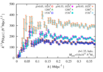
Figure 1: The measured 2D power spectra in redshift space for halo catalogues of $M_{\mathrm{min}}\!=\!5.0\!\times\!10^{11}\,h^{-1}\mathrm{M}_{\odot}$ at $z\!=\!1.35$. Open, filled and plus (cross, star) symbols show the power spectra at $\mu=0.05,\,0.55$ and 0.95, respectively. For the same $\mu$ value, three types of points show the power spectra for different mass resolution simulations with $N_{p}\!=\!1024^{3},\,1280^{3}$ and $1536^{3}$ from left to right, respectively. Error bars show FKP error estimated as $(\hat{P}+P_{\mathrm{shot}})/\sqrt{N_{\mathrm{mode}}}$ (Feldman, Kaiser & Peacock, 1994). All the data points are on the same $k$ grids but they are slightly shifted horizontally around the true $k$ values for clarity.

Finally, we average the 40 independent power spectra and obtain $P_{\mathrm{ave40}}(k,\mu)$ for matter and haloes ​.

3 RSD Model Fittings

3.1 Theoretical RSD Models

In this section we introduce four theoretical models tested in this study: two analytical models for the 2D power spectrum in redshift space, and two types of parametrization for the halo bias. We also explain how to determine the best-fitting parameters in the models through the MCMC method.

In linear theory, the 2D halo power spectrum in redshift space can be written as

$$P(k,\mu)=b^{2}(1\!+\!\beta\mu^{2})^{2}P_{\mathrm{lin}}(k)$$ (2)

(Kaiser, 1987) where $b$ is the halo bias and $P_{\mathrm{lin}}(k)$ the linear matter power spectrum in real space. We model the FoG effect arising from halo velocity dispersion by the Lorentzian-type damping function:

$$P(k,\mu)=D_{\mathrm{FoG}}(k\mu f\sigma_{\mathrm{v}})\!\times\!b^{2}(1\!+\!\beta\mu^{2})^{2}P_{\mathrm{lin}}(k)$$ (3)

$$D_{\mathrm{FoG}}(x)=\frac{1}{(1\!+\!x^{2}/2)^{2}}.$$ (4)

(Peacock & Dodds, 1994). We call this model ‘the Kaiser model’. As another model that takes into account the non-linear evolution on mildly non-linear scales, we use the model based on the perturbative expansion (Taruya et al., 2010) and generalized to biased tracers in Nishimichi & Taruya (2011):

$$P(k,\mu)=D_{\mathrm{FoG}}(k\mu f\sigma_{\mathrm{v}})$$ (5)

$$\qquad\times b^{2}\Bigl{[}P_{\delta\delta}(k)\!+\!2\beta\mu^{2}P_{\delta\theta}(k)\!+\!\beta^{2}\mu^{4}P_{\theta\theta}(k)\Bigr{.}$$

$$\qquad\qquad\qquad\qquad\qquad\Bigl{.}+bC_{A}(k,\mu;\beta)\!+\!b^{2}C_{B}(k,\mu;\beta)\Bigr{]}$$

where $P_{\delta\delta}$, $P_{\theta\theta}$ and $P_{\delta\theta}$ denote the auto power spectra of density contrast and of velocity divergence $\theta\!=\!\nabla\!\cdot\!{\mbox{\boldmath$u$}}\!=\!-\nabla\!\cdot\!{\mbox{\boldmath$v$}}/(aHf)$, and their cross power spectrum, respectively (Scoccimarro, 2004; Percival & White, 2009), and $C_{A}$ and $C_{B}$ are the correction terms arising from the higher-order mode coupling between the density and velocity fields (Taruya et al., 2010; Nishimichi & Taruya, 2011). This model is referred to as ‘the TNS model’ hereafter. It should be noted that this RSD model is strictly valid only when the halo bias is assumed to be constant. However, later we will introduce a scale-dependent halo bias to the TNS model, to incorporate the scale dependence of bias. Though there is an inconsistency here, this is probably the best approach available for the moment to get a good estimate of $f\sigma_{8}$.

For our MCMC analysis described in the next subsection, we in advance prepare templates for the power spectrum of eq. (5) at each of the three redshifts for a fiducial cosmological model. In particular, the three power spectra, $P_{\delta\delta}$, $P_{\delta\theta}$ and $P_{\theta\theta}$, are calculated by using the closure approximation up to the second-order Born approximation, and the correction terms, $C_{A}$ and $C_{B}$, are evaluated by the one-loop standard perturbation theory (Taruya & Hiramatsu, 2008; Taruya et al., 2009, 2010). In computing these templates, we use the fiducial value of the density fluctuation amplitude $\sigma_{8,\mathrm{fid}}(z\!=\!0)\!=\!0.81$ and the linear-theory growth factor at each redshift.

In the MCMC analysis, we treat $\sigma_{8}$ as a free parameter and re-scale the template spectra as follows. We replace the density and velocity spectra as $P_{ab}\rightarrow P_{ab}\!\times\!(\sigma_{8}(z)/\sigma_{8,\mathrm{input}}(z))^{2}$ and the correction terms as $C_{A}({\rm or\ }C_{B})\rightarrow C_{A}({\rm or\ }C_{B})\!\times\!(\sigma_{8}(z)/\sigma_{8,\mathrm{input}}(z))^{4}$. These replacements are valid at the leading order, and we expect that the error induced by this approximated treatment would be small. This procedure significantly saves computing time to calculate the spectra for a given value of $\sigma_{8}$.

As for the halo bias, we assume a linear bias $b\!=\!\delta_{\mathrm{halo}}/\delta_{\mathrm{matter}}$, and we adopt two models: a constant bias and a parametrized ‘Q-model’ bias to allow scale-dependence (or, equivalently, non-locality of the relation between the halo and matter density fields) (Cole et al., 2005; Nishimichi & Taruya, 2011). These are expressed as

$$b(k)=\begin{cases}\displaystyle{b_{0}}&\text{: constant bias}\\ \displaystyle{b_{0}\,\sqrt{\frac{1+Qk^{2}}{1+Ak}}}&\text{: Q-model bias},\end{cases}$$ (6)

where $b_{0}$, $Q$ and $A$ are model parameters.

To summarize, we test the following four theoretical models for the 2D halo power spectrum in redshift space: ‘Kaiser+constant bias’, ‘Kaiser+Q-model bias’, ‘TNS+constant bias’ and ‘TNS+Q-model bias’ in this study. All the models include the four parameters, $f,b_{0},\sigma_{\mathrm{v}}$ and $\sigma_{8}$. Additionally, the two models with the Q-model bias have two more parameters, $Q$ and $A$. When we analyse the matter power spectrum, we fix the bias parameters as $b_{0}\!=\!1$, and $Q\!=\!A\!=\!0$.

3.2 Fitting Methods

In this study, we employ the maximum likelihood estimation using the MCMC method and find the best-fitting model parameters as well as their allowed regions. In contrast to the analysis using the ratio of the multipole moments (e.g. Cole et al., 1994), we try to fit the shape of the 2D power spectrum, $P_{\mathrm{sim}}(k,\mu)$, directly. In such a case, we should take into account the fact that there is only a small numbers of Fourier modes in a $(k,\mu)$ bin. If the measured power spectrum $P(k,\mu)$ at each $(k,\mu)$ bin follows the Gaussian distribution, the likelihood can be written as $L\propto\exp(-\chi^{2}/2)$, where the chi-square $\chi^{2}$ is calculated in the standard manner from the measured and expected values of $P(k,\mu)$ and its standard deviation.

In reality, however, $P(k,\mu)$ does not follow the Gaussian but the chi-squared distribution even when the density contrast itself is perfectly Gaussian. In order to take into account this statistical property in the maximum likelihood estimation, we apply the Wilson-Hilferty (WH) transformation (Wilson & Hilferty, 1931) that makes a $\chi^{2}$ distribution into an approximate Gaussian. We define a new variable

$$P^{\prime}_{\mathrm{sim}}(k,\mu)=(P_{\mathrm{sim}}\!+\!P_{\mathrm{shot}})^{1/3}\ ,$$ (7)

and $P^{\prime}_{\mathrm{sim}}$ is expected to approximately obey the Gaussian distribution with a mean of

$$P^{\prime}_{\mathrm{true}}\!=\!\left[1\!-\!\frac{1}{9N_{\mathrm{mode}}}\right](P_{\mathrm{true}}\!+\!P_{\mathrm{shot}})^{1/3}$$ (8)

and a variance of

$$\sigma_{P^{\prime}}^{2}\!=\!\frac{1}{9N_{\mathrm{mode}}}(P_{\mathrm{true}}\!+\!P_{\mathrm{shot}})^{2/3}\ .$$ (9)

It should be noted that the power spectrum amplitude directly measured from the simulations, $P_{\mathrm{sim}}\!+\!P_{\mathrm{shot}}$, does not exactly obey the chi-squared distribution, because it includes the shot noise term. However, the WH transformation should be effective only at small wavenumbers where the number of modes in a $k$-space bin is small, and the shot noise term is relatively unimportant also at small wavenumbers. Therefore we adopt the above transformation, expecting that $P_{\mathrm{sim}}\!+\!P_{\mathrm{shot}}$ approximately obeys a chi-squared distribution. (For the wavenumbers where the shot noise term becomes comparable with the real-space halo power spectrum, see Fig. 8.)

Thus after this transformation, we expect that

$$\chi^{2}=\sum_{k<k_{\mathrm{max}}}\sum_{\mu}\frac{\left[P^{\prime}_{\mathrm{sim}}(k,\mu)-P^{\prime}_{\mathrm{model}}(k,\mu)\right]^{2}}{\sigma_{P^{\prime}\!,\mathrm{model}}^{2}}$$ (10)

approximately obeys a chi-squared distribution, with better accuracy than simply using $P_{\mathrm{sim}}$, where $k_{\mathrm{max}}$ is the upper bound of the range of wavenumbers that we use in fitting, $P^{\prime}_{\mathrm{model}}$ and $\sigma_{P^{\prime}_{\mathrm{model}}}$ are the WH-transformed model power spectrum and its variance given by eqs. (8) and (9) with replacing $P_{\mathrm{true}}$ by the model power spectrum $P_{\mathrm{model}}$. In our analyses, we vary $k_{\mathrm{max}}$ from $0.05$ to $0.50\,h\mathrm{Mpc}^{-1}$ at an interval of $0.05\,h\mathrm{Mpc}^{-1}$.

To see how much the fit is improved by this WH approximation, we will later compare the results with those obtained using the standard chi-square statistic calculation without the WH transformation, in which we simply use $P_{\mathrm{sim}}$, $P_{\mathrm{model}}$ and a variance of $\sigma^{2}_{P}\!=\!(P_{\mathrm{model}}\!+\!P_{\mathrm{shot}})^{2}/N_{\mathrm{mode}}$ (Feldman et al., 1994).

Then we find the best-fitting values and their allowed regions of all the model parameters (four parameters, $f,b_{0},\sigma_{\mathrm{v}}$ and $\sigma_{8}$, for the models with the constant bias, and additional two, $Q$ and $A$, for the models with the Q-model) simultaneously, by the standard MCMC technique.

4 Results and Discussion

4.1 Matter Power Spectrum

Before presenting our main results using haloes in the next subsection, let us discuss the robustness of the $f\sigma_{8}$ measurement in the absence of the halo/galaxy bias.

In the upper panel of Fig. 2, we show the matter power spectra in real space at $z\!=\!0.5$, 1.35 and 2 with the reference wavenumbers $k_{1\%}$, up to which the closure theory is expected to be accurate within 1 per cent, indicated by arrows (see Nishimichi et al., 2009; Taruya et al., 2010). The measured power spectra indeed agree with $P_{\delta\delta}$ predicted by the closure theory at $\sim\!3$ per cent level, in rough agreement with the definition of $k_{1\%}$. Therefore we use $k_{1\%}$ as indicators of a few per cent accuracy wavenumbers through the paper. In the lower panel, we show the measured $f\sigma_{8}$ values normalized by the correct ones assumed in the simulations, and the reduced chi-squared values $\chi^{2}_{\mathrm{red}}$ for the best-fitting models. It is clearly seen that $f\sigma_{8}$ from the Kaiser model (open symbols) is significantly underestimated at $k_{\max}\gtrsim 0.10\,h\mathrm{Mpc}^{-1}$ at all the redshifts, while the TNS model (filled symbols) returns $f\sigma_{8}$ closer to the correct value, with systematic errors of less than 4 per cent up to $k_{\max}\sim 0.30\,h\mathrm{Mpc}^{-1}$. As wavenumber increases, $\chi^{2}_{\mathrm{red}}$ boosts up quickly away from unity, and the maximum wavenumber $k_{\mathrm{max}}$ up to which $\chi_{\mathrm{red}}\simeq 1$ roughly coincides with $k_{1\%}$. Systematic overestimates by the TNS model are seen at $k_{\mathrm{max}}\!=\!0.20$ and $0.25\,h\mathrm{Mpc}^{-1}$ at $z\!=\!0.5$, and underestimates at $k_{\mathrm{max}}\!>\!0.15\,h\mathrm{Mpc}^{-1}$ at $z\!=\!2$. The origin of these is rather uncertain, but these might arise from sub-percent uncertainty of the power spectrum prediction by the closure theory, or from the incompleteness in the RSD modeling of the TNS model.

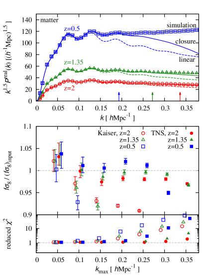
Figure 2: Upper panel: Comparison of the measured matter power spectra from simulations, with the theoretical predictions from the closure theory $P_{\delta\delta}$ (solid lines), and from a linear theory $P_{\mathrm{lin}}$ (dashed lines), at the three different redshifts. Arrows indicate the wavenumbers up to which the closure theory is accurate at 1 per cent level ($k_{\mathrm{1\%}}\!=\!0.19$, 0.27 and $0.34\,h\mathrm{Mpc}^{-1}$ at $z\!=\!0.5$, 1.35 and 2, respectively). Lower panel: The best-fitting $f\sigma_{8}$ with 1-$\sigma$ error bars and the reduced chi-squared values by fitting with the Kaiser model (open symbols) and with the TNS model (filled symbols) as a function of the maximum wavenumber $k_{\mathrm{max}}$ used in fitting. (All the data points are on the same $k_{\mathrm{max}}$ grids for the different models and redshifts, but they are slightly shifted horizontally for clarity (see also Fig. 1).

The MCMC analysis above is done with the power spectrum, $P_{\mathrm{ave40}}$, averaged over $40$ realisations. Thus, the number of modes in each of the $(k,\mu)$ bins is rather large compared with that available in realistic surveys. We therefore examine the accuracy of the RSD measurement using $\hat{P}$ in eq. (1) for each realisation.

In Fig. 3 we show by filled symbols the mean values of the best-fitting $f\sigma_{8}$ at $z\!=\!1.35$ using the TNS model, treating each of the 40 realisations as a single observation and running the MCMC chain for each of them, with and without applying the WH approximation. There can be seen overestimations of $f\sigma_{8}$ at small wavenumbers. For comparison, we also show the results from the averaged power spectrum of 40 realisations $P_{\mathrm{ave40}}$ (open symbols; same as in Fig. 2). Since the overestimating feature is greatly reduced for the results using $P_{\mathrm{ave40}}$ that includes a larger number of modes, the systematic overestimation must be caused by the small number of modes in the measured power spectrum. Then we compare the results of filled symbols with and without the WH transformation (magenta triangles versus blue circles), and it can be seen that the WH transformation improves the accuracy of $f\sigma_{8}$ estimates. Even after applying the WH transformation, there still remains a discrepancy at $k_{\mathrm{max}}\lesssim 0.10\,h\mathrm{Mpc}^{-1}$, which is likely to be the limitation of the WH transformation. (Note that the WH transformation is an approximation.) However, since the use of the WH transformation gives more accurate results than those without using it, this technique is good to be incorporated.

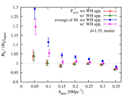
Figure 3: Systematic errors of the $f\sigma_{8}$ measurements by fitting to the matter power spectrum $P_{\mathrm{matter}}(k,\mu)$ with the TNS model at $z\!=\!1.35$. Open symbols and their error bars show the results from $P_{\mathrm{ave40}}$ (averaged power spectrum of 40 realisations) and 1-$\sigma$ statistical errors. Filled symbols show the means of 40 best-fitting $f\sigma_{8}$ values calculated for each realisation, with the errors estimated by the scatter of the $f\sigma_{8}$ values of the 40 realisations. Triangles and circles show with and without applying the Wilson-Hilferty approximation, respectively. All the data points are slightly shifted horizontally for clarity (see also Fig. 1).

Regarding the sizes of statistical errors on $f\sigma_{8}$, we also tested jackknife resampling method. Although this gives 30–70 per cent larger error bars compared to MCMC errors, we think these results are roughly consistent with each other. In the rest of the present paper, we focus on the results of the MCMC analyses after averaging over 40 power spectra (i.e., $P_{\mathrm{ave40}}$) with applying the WH transformation, to reduce the error induced by a small number of modes in $k$-space bins.

4.2 Halo Power Spectrum

4.2.1 The case of $z=1.35$ and $M_{\min}\!=\!1.0\times 10^{12}\,h^{-1}\mathrm{M}_{\odot}$

We next analyse halo catalogues to measure $f\sigma_{8}$ by fitting the power spectra in redshift space with the four analytical models. As the baseline case, we show the measured $f\sigma_{8}$ and the values of $\chi^{2}_{\mathrm{red}}$ for the best-fitting models to the halo catalogues of $M_{\min}\!=\!1.0\times 10^{12}\,h^{-1}\mathrm{M}_{\odot}$ at $z\!=\!1.35$ in Fig. 4 as a function of the maximum wavenumber, $k_{\max}$, used in the analysis. Here and hereafter, when we present results for a fixed value of $k_{\max}$, we adopt $k_{\mathrm{max}}\!=\!0.25\,h\mathrm{Mpc}^{-1}$ as the baseline value.

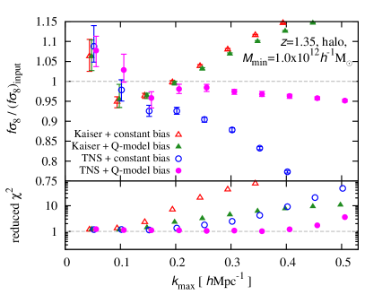
Figure 4: The best-fitting $f\sigma_{8}$ with 1-$\sigma$ error bars and the reduced chi-squared values, for the halo catalogue of $M_{\min}\!=\!1.0\times 10^{12}\,h^{-1}M_{\odot}$ at $z\!=\!1.35$. Data points show the results of the four different models of the 2D halo power spectrum: Kaiser+constant bias, Kaiser+Q-model bias, TNS+constant bias, and TNS+Q-model bias.

All the four models give $f\sigma_{8}$ within a few per cent accuracy at $k_{\mathrm{max}}\!\sim\!0.10\,h\mathrm{Mpc}^{-1}$, up to which linear theory is sufficiently accurate (see dashed lines in the upper panel of Fig. 2). There can be seen overestimation by more than 1-$\sigma$ level at $k_{\mathrm{max}}\!=\!0.05\,h\mathrm{Mpc}^{-1}$, and they are likely to be cosmic variances. We have checked that one of the two subsamples gives $f\sigma_{8}$ consistent with the correct value within 1-$\sigma$ error when we split the 40 realisations into two groups and analyse the averaged power spectra of them separately. On the other hand, underestimation at $k_{\mathrm{max}}\!=\!0.15\,h\mathrm{Mpc}^{-1}$ for all the models seem to be systematic errors. It is difficult to identify the causes of these results, since the measured power spectrum can be fitted pretty well with reduced $\chi^{2}$ values of $\sim\!1$. We leave this issue for future studies.

We then investigate the results from the four RSD modelings one by one. The Kaiser model again fails to reproduce the correct $f\sigma_{8}$ at $k_{\mathrm{max}}\!\gtrsim\!0.25\,h\mathrm{Mpc}^{-1}$, but this time $f\sigma_{8}$ are overestimated, in contrast to the results of the matter power spectra. Even when the TNS model is employed, the assumption of the constant bias leads to underestimation of $f\sigma_{8}$ at $k_{\mathrm{max}}\!\gtrsim\!0.20\,h\mathrm{Mpc}^{-1}$. However, when we use the TNS model with the scale-dependent Q-model bias, the systematic error is significantly reduced down to 5 per cent level up to $k_{\max}\!\sim\!0.50\,h\mathrm{Mpc}^{-1}$. Note that the adopted perturbation theory is accurate by $\sim\!1$ per cent level only up to $k_{\mathrm{max}}=0.27\,h\mathrm{Mpc}^{-1}$. It is rather surprising that the reduced $\chi^{2}$ values are $\sim 1$ up to $k_{\max}\!\sim\!0.50\,h\mathrm{Mpc}^{-1}$. This means that $\sim 5$ per cent level systematic errors of $f\sigma_{8}$ is possible even if the fit looks good, which should be kept in mind in future analyses applied on the real data.

We plot in Fig. 5 the four best-fitting model power spectra against the simulation data measured at three fixed direction cosine of the wavevector, $\mu\!=\!0.05$, 0.55 and $0.95$. In Fig. 6, the halo bias measured from N-body simulations is presented. The plot shows the mean of the 40 independently-measured biases from each realisation in real space as $b(k)\!=\!\sqrt{P_{\mathrm{halo}}(k)/P_{\mathrm{matter}}(k)}$, and its standard deviation. For comparison, we also show the best-fitting model bias curves, $b(k)\sigma_{8}/\sigma_{8,\mathrm{input}}$, for the four models, which are calculated for each model with the corresponding parameters, $b_{0},Q,A$ and $\sigma_{8}$, using their best-fitting values found by the MCMC analysis. The measured bias shows a monotonic increasing trend with the wavenumber. Generally the scale-dependence of the halo bias is different for different halo mass and redshift, and both increasing and decreasing trends are possible depending on these parameters (Sheth & Tormen 1999; Okumura & Jing 2011; Nishimichi & Taruya 2011).

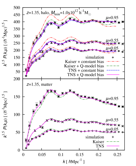
Figure 5: The power spectra in redshift space at $\mu\!=\!0.05$, 0.55 and 0.95 at $z\!=\!1.35$. The upper panel is for the halo catalogue of $M_{\min}\!=\!1.0\times 10^{12}h^{-1}\,\mathrm{M}_{\odot}$, while the lower panel is for the matter distribution. The data points are measurements from simulations and the curves show the best fits for different models (see labels in the figure for corresponding models).

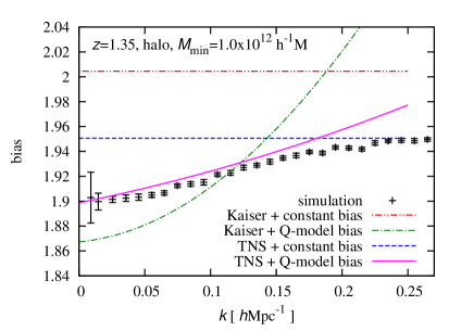
Figure 6: Comparison between the halo bias directly measured from simulations and the best-fitting bias models, for the halo catalog of $M_{\min}\!=\!1.0\times 10^{12}\,h^{-1}\mathrm{M}_{\odot}$ at $z\!=\!1.35$. The data points and lines are for the same simulation and models as those in the upper panel of Fig. 5.

When the Kaiser model is used, an apparently inverse trend is seen for the systematic deviation of $f\sigma_{8}$ measurements from the input value, for the matter and halo power spectra, and this can be understood as follows. In a fitting to the matter spectrum, the Kaiser model tries to reproduce the power enhancement arising from the non-linear evolution at high-$k$ by setting $\sigma_{8}$ larger than the input value, because of the absence of the bias model parameters (see dash-dotted line at $\mu\sim 0$ in the lower panel of Fig. 5). It is easy to show that, from the Kaiser formula, a systematically lower value of $f\sigma_{8}$ than the input value is favored to reproduce the RSD effect at large $\mu$, when $\sigma_{8}$ is overestimated. In a fitting to the halo spectrum, there are degrees of freedom for bias models, but the non-linear power enhancement at high-$k$ cannot be completely absorbed by the constant or Q-model bias. The power enhancement can also be absorbed to some extent by reducing $\sigma_{\mathrm{v}}$ in the FoG damping factor, but Fig. 7 indicates that the best-fitting $\sigma_{\mathrm{v}}$ is zero when the Kaiser model is employed, regardless of the bias modelings. The power enhancement that cannot be absorbed by bias modelings or the FoG parameter then favors a larger $f\sigma_{8}$ than the correct value, at the cost of a poorer agreement at low-$k$.

The systematic underestimation of $f\sigma_{8}$ when we employ the TNS+constant bias model might be a result of the discrepancy between the correct bias measured directly from simulations and the best-fitting constant bias at low-$k$ ($k\lesssim 0.15\,h\mathrm{Mpc}^{-1}$, see dashed line in Fig. 6), because the bias shape of the best-fitting model of the TNS+Q-model bias is close to the simulation-measured bias.

Compared with the sizes of statistical errors for the Kaiser+constant bias model, we get nearly equal sizes of errors for the Kaiser+Q-model bias, 1.5–2 times larger errors for the TNS+constant bias and 2.5 times larger errors for the TNS+Q-model bias. The size of statistical error becomes generally larger with increasing the number of fitting model parameters because of the effect of marginalising, though the size of increase is quantitatively different for different models because of different ways of parameter degeneracy.

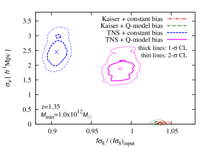
Figure 7: The best-fitting values and the 1- and 2-$\sigma$ confidence regions of the four different models (see figure) in the $f\sigma_{8}$-$\sigma_{\mathrm{v}}$ plane, for the halo catalogue of $M_{\min}\!=\!1.0\times 10^{12}h^{-1}\mathrm{M}_{\odot}$ at $z\!=\!1.35$.

4.2.2 Dependence on $z$ and $M_{\min}$

Then we investigate the other halo catalogues at the three redshifts with different minimum halo mass thresholds. The results of the $f\sigma_{8}$ measurement by fitting with the TNS+Q-model bias are shown in Fig. 8. We firstly focus on the results at $k_{\mathrm{max}}\!\sim\!k_{1\%}$. In this regime $f\sigma_{8}$ measurements with systematic uncertainties of less than $\!\sim\!5$ per cent are achieved, except for massive halo catalogues of $M_{\min}\!\gtrsim\!10^{13}\,h^{-1}\mathrm{M}_{\odot}$ at $z\!=\!2$. These correspond to highly​ biased haloes of $b_{0}\sigma_{8}/\sigma_{8,\mathrm{input}}\gtrsim\!4$. Therefore we can state that the TNS model can be used for $f\sigma_{8}$ measurements with an accuracy of 5 per cent if $k_{\max}\sim k_{1\%}$ and $b\lesssim\!4$.

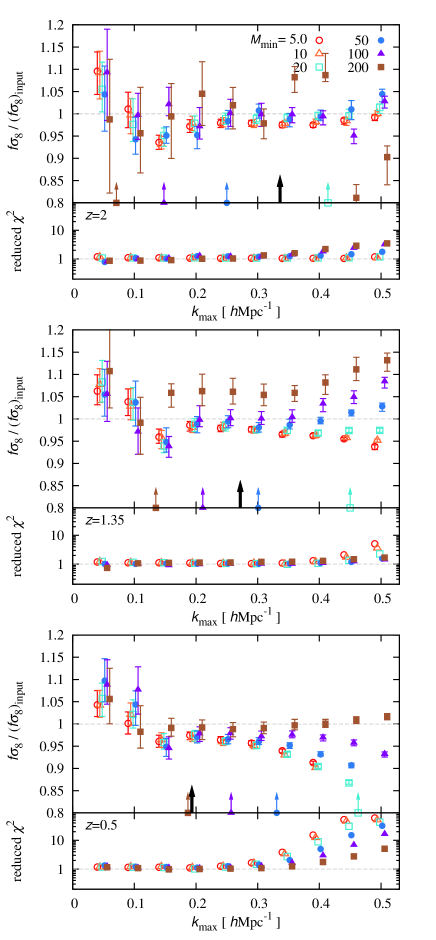
Figure 8: The best-fitting $f\sigma_{8}$ and the reduced chi-squared values at $z\!=\!2$, 1.35 and 0.5 from top to bottom, respectively. Different symbols are for the different values of the minimum halo mass $M_{\mathrm{min}}\!=\!5.0$, 10, 20, 50, 100 and 200 in units of $10^{11}\,h^{-1}\mathrm{M}_{\odot}$. Black arrows show the $k_{1\%}$ wavenumbers. Cyan, blue, purple and blown arrows with symbols indicate the wavenumbers where the shot noise term becomes comparable with the halo power spectrum in real space, for the catalogues of $M_{\mathrm{min}}\!=\!20$, 50, 100 and 200, respectively (see, Sec. 3.2).

The behavior beyond $k_{1\%}$ depends on the mass of haloes as well as redshift. In some cases, a value of $f\sigma_{8}$ consistent with its input value is successfully recovered up to much higher wavenumbers (see e.g., the heaviest halo catalogue at $z\!=\!0.5$, from which we can measure the correct $f\sigma_{8}$ values up to $k_{\mathrm{max}}\!=\!0.45\,h\mathrm{Mpc}^{-1}$). However this result should be taken with care. This apparently successful recovery of $f\sigma_{8}$ is probably because of the rather flexible functional form of the scale-dependent bias adopted in this paper. The parameters $A$ and $Q$ can sometimes absorb the mismatch between the true matter power spectra and the TNS model beyond $k_{1\%}$ without leaving systematics to $f\sigma_{8}$ for some special cases. The situation would probably be quite different when different parameterizations are chosen for $b(k)$. Nevertheless, it is of interest to explore the possibility to add some more information from higher wavenumbers. Although we, in this paper, employ only one particular functional form for the scale-dependent bias as well as a constant bias model, the reproductivity of the growth-rate parameter from high-$k$ modes with different bias functions is also of interest. We leave further investigations along this line for future studies.

4.3 Implications for Future Surveys

In this subsection, we give some implications for future use of our analysis methodologies. As seen above, we have demonstrated that we can measure $f\sigma_{8}$ with a systematic error of $\!\lesssim\!5$ per cent by using the TNS model combined with the Q-model bias, provided that the used wavenumber range is $k_{\max}\!\sim\!k_{1\%}$ and haloes are not strongly biased ($b\lesssim\!4$).

Nishimichi & Taruya (2011) showed the expected constraints on the growth rate $f(z)$ for some on-going and planned surveys (fig. 6 and table III in their paper). The estimated 1-$\sigma$ statistical errors are 7.5–3.9 per cent at redshift $z\!=\!0.7$–$1.5$ for SuMIRe-PFS, and 5.1 per cent at $z\!=\!3.0$ for HETDEX. This means that the TNS+Q-model bias fit can reduce the systematic errors arising from the non-linear effects and the halo bias to be comparable or lower than the statistical errors from these surveys.

The space mission Euclid will survey over a redshift range of $0.7\!<\!z\!<\!2.1$ and get redshifts of 50 million galaxies. The number of galaxies in each redshift bin will be more than one million. We can roughly estimate the statistical error expected from Euclid to be a few per cent level, by using an empirical formula

$$\frac{\Delta f\sigma_{8}}{\!f\sigma_{8}}\!\sim\!\frac{50}{\sqrt{N_{\mathrm{gal}}}}$$ (11)

(Guzzo, 2008; Song & Percival, 2009) where $N_{\mathrm{gal}}$ is the number of galaxies. This estimation indicates that we need to further improve the modeling of RSD, to make the systematic error smaller than the statistical error of Euclid.

5 Conclusions

We have investigated how accurately the structure growth rate $f\sigma_{8}$ can be measured from the RSD effects through the model fittings. We have used the halo catalogues generated from N-body simulations assuming the standard $\Lambda$CDM universe with general relativity, at $z\!=\!0.5$, 1.35 and 2 for various minimum halo mass thresholds of $5.0\times 10^{11}$– $2.0\times 10^{13}\,h^{-1}\mathrm{M}_{\odot}$. We have tested two analytical models for the 2D power spectrum in redshift space: the Kaiser model and the TNS model including the higher-order coupling terms between the density and velocity fields. We have implemented two models for the halo bias: a constant bias and a scale-dependent parametric bias model (i.e., Q-model).

We find significant systematic error (more than 10 per cent for $k_{\max}\!\gtrsim\!0.30\,h\mathrm{Mpc}^{-1}$) when the Kaiser model is simply adopted regardless of the bias modelings, which is consistent with previous studies. Under the assumption of the constant bias, the systematic error still remains even when we employ the TNS model. However, when we use the TNS model with the Q-model bias, the systematic error can be reduced to $\lesssim\!$ 5 per cent for all the redshifts and mass thresholds, by using the wavenumber range up to $k_{1\%}$ (e.g. $k_{1\%}\!=\!0.19$, 0.27 and $0.34\,h\mathrm{Mpc}^{-1}$ at $z\!=\!0.5$, 1.35 and 2, respectively).

For some heavy halo catalogues at $z\!=\!0.5$, the TNS+Q-model gives the accurate $f\sigma_{8}$ measurement significantly beyond $k_{1\%}$. This is probably because the Q-model bias model absorbs the difference between the simulated matter power spectrum and the TNS model prediction, but this feature is only for particular cases, and a further investigation is necessary. At lower mass ranges, the TNS+Q-model gives clearly biased $f\sigma_{8}$ estimates at $k_{\mathrm{max}}\!>\!k_{1\%}$, especially at lower redshifts where the non-linear effects are more significant.

We conclude that the TNS model as a 2D power spectrum formula combined with the Q-model bias is a powerful tool to measure the structure growth rate. The systematic error can be reduced to under 5 per cent at $k_{\max}\!\sim\!k_{1\%}$, which is comparable with or smaller than the expected statistical errors of near-future ground-based surveys at high redshifts, such as SuMIRe-PFS and HETDEX. Some future ambitious surveys, such as Euclid, will achieve even smaller statistical errors, and we will need to pursue more accurate theoretical models taking into account the non-linear effects and the halo/galaxy bias. We also note that the TNS formula is valid only when gravity is described by general relativity. Therefore this model cannot be used for a test of other theories of gravity, but still it can be used to test whether general relativity is a valid theory to describe the formation of large-scale structure.

Finally, we note on the importance of an appropriate treatment for the $f\sigma_{8}$ measurement, when only a small number of Fourier modes are available in a $k$-space bin of power spectrum measurements. In such a case, a measured power spectrum $\hat{P}$ in eq. (1) obeys not the Gaussian but the chi-squared distribution even when the underlying density field itself obeys the Gaussian statistics. In this study, we have introduced the WH transformation which converts the variable obeying the chi-squared distribution into an approximate Gaussian, in our likelihood calculation of the MCMC analysis. Indeed we have confirmed that the WH transformation improves the accuracy of the $f\sigma_{8}$ measurement, and hence it is a useful prescription when the number of available modes is small.

References

- Beutler et al. (2013) Beutler F. et al., 2013, MNRAS, 429, 3604
- Bianchi et al. (2012) Bianchi D., Guzzo L., Branchini E., Majerotto E., de la Torre S., Marulli F., Moscardini L., Angulo R. E., 2012, MNRAS, 427, 2420
- Bielby et al. (2013) Bielby R. et al., 2013, MNRAS, 430, 425
- Blake et al. (2004) Blake C. et al., 2011, MNRAS, 415, 2892
- Cole et al. (1994) Cole S., Fisher K. B., Weinberg D. H., 1994, MNRAS, 267, 785
- Cole et al. (2005) Cole S. et al., 2005, MNRAS, 362, 505
- Contreras et al. (2013a) Contreras C. et al., 2013, MNRAS, 430, 924
- Contreras et al. (2013b) Contreras C., Blake C., Poole G. B., Marin F., 2013, MNRAS, 430, 934
- de la Torre & Guzzo (2011) de la Torre S., Guzzo L., MNRAS, 427, 327
- de la Torre et al. (2013) de la Torre S. et al., 2013, A&A, in press
- Feldman et al. (1994) Feldman H. A., Kaiser N., Peacock J. A., 1994, ApJ, 426, 23
- Fisher et al. (1994) Fisher K. B. et al., 1994, MNRAS, 267, 927
- Guzzo (2008) Guzzo L., 2008, Nature, 451, 541
- Hamilton (1998) Hamilton A. J. S., 1998, ASSL, 231, 185S
- Hatton & Cole (1998) Hatton S., Cole S., 1998, MNRAS, 296, 10
- Hockney & Eastwood (1988) Hockney R. W., Eastwood J. W., 1988, Computer simulation using particles, Bristol: Hilger 1988
- Jackson (1972) Jackson J. C., 1972, MNRAS, 156, 1P
- Jennings, Baugh & Pascoli (2011a) Jennings E., Baugh C. M., Pascoli S., 2011a, MNRAS, 410, 2081
- Jennings, Baugh & Pascoli (2011b) Jennings E., Baugh C. M., Pascoli S., 2011b, ApJ, 727, L9
- Kaiser (1987) Kaiser N., 1987, MNRAS, 227, 1
- Komatsu et al. (2011) Komatsu E. et al., 2011, ApJS, 192, 18
- Kwan, Lewis & Linder (2012) Kwan J., Lewis G. F., Linder E. V., 2012, ApJ, 748, 78
- Lewis, Challinor & Lasenby (2000) Lewis A., Challinor A., Lasenby A., 2000, ApJ, 538, 473
- Nishimichi et al. (2009) Nishimichi T. et al., 2009, PASJ, 61, 321