Constraining cosmic string parameters with curl mode of CMB lensing

Abstract

We present constraints on a cosmic string network with a measurement of weak gravitational lensing from CMB temperature map. The cosmic string network between observer and last scattering surface of CMB photons generates vector and/or tensor metric perturbations, and the deflection of CMB photons by these gravitational fields has curl mode which is not produced by the scalar metric perturbations. In this paper, we use the power spectrum of curl mode obtained from Planck to constrain the string tension, $G\mu$, and the reconnection probability, $P$. In demonstrating the parameter constraints with Planck curl mode, we also measure the lensing power spectrum from the Atacama Cosmology Telescope (ACT) 2008 season data, which have better angular resolution with lower instrumental noise on a much smaller chunk of the sky. Assuming $P=1$, the upper bound on tension is $G\mu=6.6\times 10^{-5}$ with $2\sigma$  (95% C.L.), using curl mode from Planck, which is weaker than that from the small-scale temperature power spectrum. For small values of $P$, however, the constraint from curl mode becomes tighter compared to that from temperature power spectrum. For $P\raise 2.9pt\hbox{$\scriptstyle<$}\lower 0.5pt\hbox{$\scriptscriptstyle\sim$}\;10^{-2}$, we obtain the constraint on the combination of the string parameters as $G\mu P^{-1}\leq 3.4\times 10^{-5}$ at more than $2\sigma$  (95% C.L.).

I Introduction

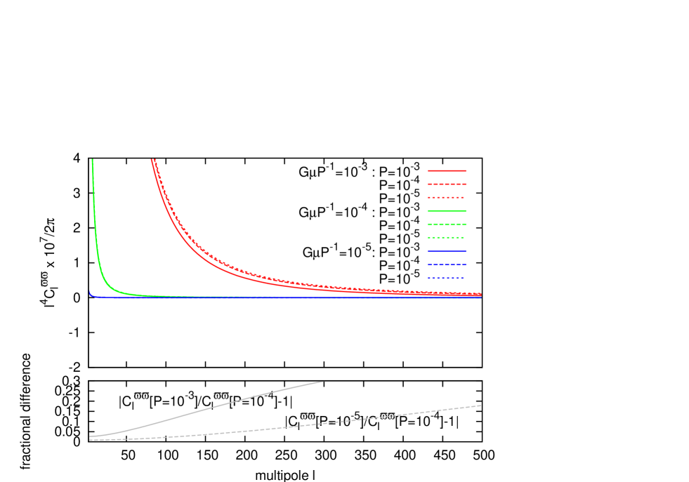
Figure 1: Theoretical angular power spectra of curl mode for different values of the combination of the cosmic string parameters with $G\mu P^{-1}=10^{-3}$ (red), $10^{-4}$ (green), $10^{-5}$ (blue). For each value of $G\mu P^{-1}$, we show the case with different values of the reconnection probability, i.e., $P=10^{-3}$ (solid), $10^{-4}$ (dashed), $10^{-5}$ (dotted). The bottom panel shows the fractional difference between the angular power spectra with the different values of $P$.

At arcminute scales, CMB anisotropies are perturbed significantly by gravitational lensing. Recently, several groups have reported the detection of lensing signals by reconstructing lensing fields involved in the CMB anisotropies, using CMB maps alone or the cross correlations between CMB and other observables (Smith07, ; Hirata:2008cb, ; Das:2011ak, ; vanEngelen:2012va, ; Bleem:2012gm, ; Sherwin:2012mr, ; Das:2013zf, ; Ade:2013tyw, ; Ade:2013aro, ; Hanson:2013daa, ). The lensing signals measured from ongoing, upcoming and next-generation CMB experiments, e.g., Planck PLANCK , SPTpol SPTPol , PolarBear POLARBEAR , ACTPol Niemack:2010wz , COrE Bouchet:2011ck , PRISM Andre:2013afa and CMBPol Smith:2008an , will have enough sensitivity to probe several fundamental issues, such as properties of dark energy and massive neutrinos (e.g., Hu:2001fb ; Lesgourgues:2006nd ; dP09 ; Namikawa:2010re ; Das:2011mf ).

The lensing effect on the temperature anisotropies is described by a remapping of the primary anisotropies. Denoting the primary temperature anisotropies at position $\widehat{\bm{n}}$ on the last scattering surface, $\Theta(\widehat{\bm{n}})$, the lensed temperature anisotropies are given by

$$\widetilde{\Theta}(\widehat{\bm{n}}) =\Theta(\widehat{\bm{n}}+\bm{d}(\widehat{\bm{n}}))$$

$$=\Theta(\widehat{\bm{n}})+\bm{d}(\widehat{\bm{n}})\cdot\bm{\nabla}\Theta(\widehat{\bm{n}})+\mathcal{O}(|\bm{d}|^{2})\,.$$ (1)

The vector, $\bm{d}(\widehat{\bm{n}})$, is the deflection angle, and, in terms of parity, we can decompose it into gradient (even parity) and curl (odd parity) modes Hirata:2003ka ; Cooray:2005hm ; Namikawa:2011cs :

$$\bm{d}(\widehat{\bm{n}})=\bm{\nabla}\phi(\widehat{\bm{n}})+(\star\bm{\nabla})\varpi(\widehat{\bm{n}})\,,$$ (2)

where the symbol, $\star$, denotes an operation which rotates the angle of a two-dimensional vector counterclockwise by $90$ degrees.

It is known that scalar metric perturbations such as the matter density fluctuations at linear order produce the gradient mode, but do not generate the curl mode. At linear order, the curl mode is induced by only vector and/or tensor metric perturbations. Thus, the curl mode is a probe of nonscalar metric fluctuations.

In this paper, among various active seeds of nonscalar metric perturbations, we are particularly interested in cosmic strings. They can be generally formed as topological defects in the early Universe through a symmetry breaking phase transition. There has been a renewed interest in another possibility that F and D strings of superstring theory can appear at the end of stringy inflation and act as cosmic strings, so-called cosmic superstrings. The evolution of cosmic superstrings may differ from that of ordinary field-theoretic strings, because the reconnection probability $P$ may be significantly smaller than unity. While the ordinary strings always reconnect when they intersect, the reconnection probability of cosmic superstrings is typically in the range $10^{-3}\lesssim P\lesssim 1$. Moreover, $P$ strongly depends on the details of the compactification. For a hybrid network that contains bound states, the situation is more complicated and $P$ can vary from $0$ to $1$ Copeland:2003bj ; Jackson:2004zg . Hence, the constraint on $P$ plays an important role in distinguishing between ordinary cosmic strings and cosmic superstrings.

According to our previous work Namikawa:2011cs ; Yamauchi:2012bc ; Yamauchi:2013fra , cosmic strings can produce an observable curl mode for small values of $P$. Detection of a curl mode in the CMB lensing deflection would provide strong evidence for cosmic strings. An interesting point is that the lensing curl mode is more sensitive to small values of the reconnection probability compared to the temperature angular power spectrum induced by the Gott-Kaiser-Stebbins (GKS) effect Kaiser:1984 ; Gott:1985 . These two probes from CMB observation would have complementarity for constraining cosmic string parameters Yamauchi:2013prep . In this paper, using the angular power spectrum of the curl modes, we present constraints on cosmic string parameters. In our analysis of parameter constraints, we use the curl-mode power spectrum from Planck. In demonstrating the results obtained from Planck data, we also measure the lensing power spectrum from the ACT data, which have better angular resolution with lower instrumental noise on a much smaller chunk of the sky.

This paper is organized as follows. In Sec. II, we briefly review a cosmic string network and its effect on the curl-mode power spectrum. In Sec. III, our curl-mode data for constraining cosmic string parameters are described, and the method for obtaining our curl-mode power spectrum is explained. In Sec. IV, we show the curl-mode power spectra used in our analysis, and in Sec. V, the results of constraints on cosmic-string parameters are shown. Sec. VI is devoted to summary and discussion of future prospects.

II Curl mode from cosmic string network

Cosmic strings continuously produce not only scalar perturbations but also vector and tensor perturbations, and induce curl modes Namikawa:2011cs ; Yamauchi:2012bc (and also B-mode shear Yamauchi:2012bc and rotation Thomas:2009bm in galaxy images). The amplitudes of the curl modes are typically determined by the dimensionless string tension $G\mu$ . In this paper, we focus on the contributions from vector perturbations since those from tensor perturbations are negligible in the curl mode for the scales of our interest Yamauchi:2013fra .

The curl-mode angular power spectrum induced by vector perturbations in general has the following form Yamauchi:2012bc ; Yamauchi:2013fra :

$$C_{\ell}^{\varpi\varpi}=4\pi\frac{(\ell-1)!}{(\ell+1)!}\int^{\infty}_{0}\frac{{\rm d}k}{k}\biggl{[}\int^{\chi_{*}}_{0}\frac{{\rm d}\chi}{\chi}\Delta_{1}(k,\chi)j_{\ell}(k\chi)\biggr{]}^{2}\,,$$ (3)

where $\chi_{*}$ denotes the conformal distance at the last scattering surface and $\Delta_{1}(k,\chi)$ is the dimensionless auto power spectrum of the vector perturbations. Note that the curl-mode power spectrum given above has originally involved the unequal-time power spectrum. Here, to evaluate the integral analytically, we adopt the factorizable ansatz that the unequal-time power spectrum is described by the square root of the product of auto power spectra given at different times.

To compute the string-induced power spectrum, we consider a string network described by the velocity-dependent one-scale model (VOS) Martins:1996jp ; Martins:2000cs ; Avgoustidis:2005nv ; Takahashi:2008ui ; Yamauchi:2010ms ; Yamauchi:2010vy , which is characterized by the correlation length $\xi=1/H\gamma$ and the root-mean-square velocity $v$ . Here $H$ denotes the Hubble expansion rate. In the VOS, the reconnection process is required for the energy loss of the network through loop formation and the approach to the scaling solution, in which the correlation length scales with the Hubble radius. Thus, observables associated with the global properties of the network sensitively depend on the reconnection probability, and $\gamma$, $v$ in the scaling regime are in fact well approximated by $\gamma\approx(\pi\sqrt{2}/3\tilde{c}P)^{1/2}$ , $v^{2}\approx(1/2)(1-\pi/(3\gamma))$ for $\tilde{c}P\ll 1$ , where $\tilde{c}\approx 0.23$ quantifies the efficiency of the loop formation  Martins:2000cs . If $G\mu$ and $P$ are given, the quantities, $\xi$ and $v$, are evaluated, and then the power spectrum induced by cosmic strings is computed as

$$\Delta_{1}^{2}(k,\chi) =(16\pi G\mu)^{2}\frac{\sqrt{6\pi}v^{2}}{12(1-v^{2})}$$

$$\qquad\times\frac{4\pi k^{3}\chi^{2}a^{4}}{H}\left(\frac{a}{k\xi}\right)^{5}{\rm erf}\left(\frac{k\xi/a}{2\sqrt{6}}\right)\,.$$ (4)

The above equation implies that the angular power spectrum given in Eq. (3) roughly scales as $C_{\ell}^{\varpi\varpi}\propto(G\mu)^{2}P^{-2}$  at the large-scale limit ($\ell\to 0$), where the curl-mode signals become significant.

In Fig. 1, to see the dependence of curl mode on $G\mu$ and $P$, we show the expected angular power spectrum for the curl mode with a combination of parameters, $G\mu P^{-1}=10^{-3}$ (red), $10^{-4}$ (green), $10^{-5}$ (blue). For each case of $G\mu P^{-1}$, we change the values of the reconnection probability as $P=10^{-3}$ (solid), $10^{-4}$ (dashed), and $10^{-5}$ (dotted). The bottom panel shows the fractional difference between the angular power spectra with the different values of $P$. The string-induced curl mode has large amplitude at large-angular scales. As expected, for the same value of $G\mu P^{-1}$, the curl-mode power spectra at large scales are hardly distinguishable. Hence, measurement of the curl mode gives constraints on the combination of string parameters $G\mu P^{-1}$ .

III Data and Analysis

To constrain cosmic string parameters, we use the curl-mode power spectrum measured from two independent data sets. The first set of curl-mode data we use in this paper is obtained from Planck Ade:2013tyw , a satellite CMB experiment. The curl mode obtained from Planck has the highest signal-to-noise ratio in the currently available CMB data. The resultant curl-mode power spectrum from Planck, however, may be affected by, e.g., residual contaminations from foregrounds and analysis of lensing reconstruction. As a second data set, we derive a curl-mode power spectrum estimate from a public ACT temperature map, and the details are described below. Since ACT has high angular resolution and sensitive to temperature fluctuations at smaller scales compared to Planck, the systematics involved in the ACT data would be different from that in the Planck data. In this respect, the results obtained from the ACT data can be utilized as a cross-check of the Planck results. The measured curl mode obtained from ACT is useful to understand how the constraints on cosmic string parameters depend on the sensitivity of CMB experiments to the curl-mode signal. In Secs. III.1 and III.2, we briefly summarize the method for estimating the curl-mode power spectrum from the ACT and Planck temperature maps, respectively.

III.1 ACT

III.1.1 Temperature map

For lensing reconstruction, we use the full map with point source subtraction, taken from the LAMBDA website LAMBDA , observed at 148 GHz in the 2008 season, covering 845.6 deg² of the sky Dunner:2012vp . Choosing a region where the noise level is lower than $\sim 35\,\mu$K-arcmin, the full map is divided into four rectangular regions as follows. The coordinate of the center for $i$th map ($i=1$ - $4$) is given by $(1500+1920\times i,588)$ in grid space. The area of each quarter map is $16\times 4$ deg² (where the size of each pixel is $0.5$ arcmin-square). To mitigate survey boundary effects, we apply an apodization window function following Ref. Namikawa:2012pe :

$$W(x,y;s_{0})=w(x;s_{0})w(y;s_{0})\,.$$ (5)

We use a sine apodization function given by

$$w(s;s_{0}) =w_{0}\times\begin{cases}1&|s|<as_{0}\\ \sin\left(\dfrac{\pi}{2}\dfrac{1-|s|/a}{1-s_{0}}\right)&as_{0}\leq|s|<a\\ 0&a\leq|s|\end{cases}\,,$$ (6)

with $w_{0}=(2a[s_{0}+2(1-s_{0})/\pi])^{-1}$. Note that the parameter, $s_{0}$, indicates the width of the region where the apodization is applied. Throughout this paper, we choose $s_{0}=0.0$.

III.1.2 Lensing potential estimator

The estimator for the lensing potentials, $\widehat{x}_{\bm{\ell}}$ ($x=\phi$ or $\varpi$), can be constructed using the statistical anisotropy generated by lensing (see e.g., Refs. Zaldarriaga:1998te ; Hu:2001kj for gradient mode, and Refs. Cooray:2005hm ; Namikawa:2011cs for curl mode). A naive estimator, however, suffers from a so-called “mean-field bias,” i.e., nonzero mean of the estimator in the presence of masking, inhomogeneous noise and so on. The mean-field bias needs to be corrected with some methods.

In our analysis, to reduce the mean-field bias, we use the following estimator Namikawa:2012pe :

$$\widehat{x}_{\bm{L}} =\mathcal{A}_{L}^{xx}{\int\!\!\frac{\,{\rm d}^{2}\bm{\ell}\,}{(2\pi)^{2}}\,}\frac{\mathcal{F}^{x}_{\bm{L},\bm{\ell}}}{2\widehat{C}^{\Theta\Theta}_{\ell}\widehat{C}^{\Theta\Theta}_{|\bm{L}-\bm{\ell}|}}\widehat{\Theta}_{\bm{\ell}}\widehat{\Theta}_{\bm{L}-\bm{\ell}}\,.$$ (7)

The quantity, $\widehat{\Theta}_{\bm{\ell}}$, is the beam-deconvolved observed map in Fourier space and expressed as $\widehat{\Theta}_{\bm{\ell}}=\widetilde{\Theta}_{\bm{\ell}}+B_{\ell}^{-1}n_{\bm{\ell}}$, with $B_{\ell}$ denoting the isotropic beam transfer function, taken from the LAMBDA website LAMBDA , and $n_{\bm{\ell}}$ describing the instrumental noise as well as contaminations from unresolved point sources. The quantity $\widehat{C}^{\Theta\Theta}_{\ell}$ is the temperature angular power spectrum measured directly from each map. The weight function and normalization are defined as

$$\mathcal{F}_{\bm{L},\bm{\ell}}^{x} =\sum_{a=x,\epsilon,s}\frac{A_{L}^{aa}\{{\bm{\mathrm{R}}}_{L}^{-1}\}^{xa}}{A_{L}^{xx}\{{\bm{\mathrm{R}}}_{L}^{-1}\}^{xx}}F_{\bm{L},\bm{\ell}}^{a}\,,$$ (8)

$$\mathcal{A}_{L}^{xx} =\{{\bm{\mathrm{R}}}_{L}^{-1}\}^{xx}A_{L}^{xx}\,.$$ (9)

Note that the indexes, $\epsilon$ and $s$, represent the effect of inhomogeneous reionization, Doppler boosting, and of additional contaminations such as inhomogeneous noise and unresolved point sources, respectively (see Ref. Namikawa:2012pe for details). The quantity, ${\bm{\mathrm{R}}}_{L}$, is the $3\times 3$ response matrix whose elements are

$$R_{L}^{ab}=\frac{A_{L}^{aa}}{A_{L}^{ab}}\,;\,A_{L}^{ab}=\left\{{\int\!\!\frac{\,{\rm d}^{2}\bm{\ell}\,}{(2\pi)^{2}}\,}\frac{F_{\bm{L},\bm{\ell}}^{a}F_{\bm{L},\bm{\ell}}^{b}}{2\widehat{C}^{\Theta\Theta}_{\ell}\widehat{C}^{\Theta\Theta}_{|\bm{L}-\bm{\ell}|}}\right\}^{-1}\,,$$ (10)

where the weight functions are given by

$$F^{\phi}_{\bm{L},\bm{\ell}} =[\widetilde{C}^{\Theta\Theta}_{\ell}\bm{L}\cdot\bm{\ell}+\widetilde{C}^{\Theta\Theta}_{|\bm{L}-\bm{\ell}|}\bm{L}\cdot(\bm{L}-\bm{\ell})]$$

$$F^{\varpi}_{\bm{L},\bm{\ell}} =[\widetilde{C}^{\Theta\Theta}_{\ell}(\star\bm{L})\cdot\bm{\ell}+\widetilde{C}^{\Theta\Theta}_{|\bm{L}-\bm{\ell}|}(\star\bm{L})\cdot(\bm{L}-\bm{\ell})]$$

$$F^{\epsilon}_{\bm{L},\bm{\ell}} =-\widehat{C}^{\Theta\Theta}_{\ell}-\widehat{C}^{\Theta\Theta}_{|\bm{L}-\bm{\ell}|}\,,$$

$$F^{s}_{\bm{L},\bm{\ell}} =1\,,$$ (11)

with $\delta_{\bm{0}}\widetilde{C}^{\Theta\Theta}_{\ell}=\langle|\widetilde{\Theta}_{\bm{\ell}}|^{2}\rangle$ denoting the lensed temperature angular power spectrum, computed by CAMB Lewis:1999bs with fiducial cosmological parameters from ACT+WMAP data Dunkley:2010ge . Note that, for curl mode, since $R^{\varpi\epsilon}_{\ell}=R^{\varpi s}_{\ell}=0$, we find $\mathcal{F}_{\bm{\ell},\bm{L}}^{\varpi}=F_{\bm{\ell},\bm{L}}^{\varpi}$ and $\mathcal{A}_{\ell}^{\varpi\varpi}=A_{\ell}^{\varpi\varpi}$.

III.1.3 Lensing power spectrum estimate: Bias-hardened estimator

With the estimators for lensing fields described above, the lensing power spectrum, $\widehat{C}^{xx}_{L}$, is estimated as Namikawa:2012pe ; Ade:2013tyw

$$\widehat{C}^{xx}_{L}={\int_{0}^{2\pi}\!\!\frac{\,{\rm d}\varphi_{\bm{L}}\,}{2\pi}\,}[|\widehat{x}_{\bm{L}}|^{2}-\widehat{N}^{xx}_{\bm{L}}]\,,$$ (12)

with $\varphi_{\bm{L}}$ denoting the angle of multipole vector, $\bm{L}$. Hereafter, we call the above estimator the bias-hardened estimator (BHE). The second term in the above equation (12), usually referred to as the “Gaussian bias,” is estimated through Namikawa:2012pe

$$\widehat{N}^{xx}_{\bm{L}} =\left(\mathcal{A}_{L}^{xx}\right)^{2}{\int\!\!\frac{\,{\rm d}^{2}\bm{\ell}\,}{(2\pi)^{2}}\,}{\int\!\!\frac{\,{\rm d}^{2}\bm{\ell}^{\prime}\,}{(2\pi)^{2}}\,}$$

$$\times\frac{\mathcal{F}^{x}_{\bm{L},\bm{\ell}}\mathcal{F}^{x}_{\bm{L},\bm{\ell}^{\prime}}}{\widehat{C}^{\Theta\Theta}_{\ell}\widehat{C}^{\Theta\Theta}_{|\bm{L}-\bm{\ell}|}\widehat{C}^{\Theta\Theta}_{\ell^{\prime}}\widehat{C}^{\Theta\Theta}_{|\bm{L}-\bm{\ell}^{\prime}|}}$$

$$\times\left({\bm{\mathrm{C}}}_{\bm{\ell},\bm{L}-\bm{\ell}^{\prime}}\widehat{\Theta}_{\bm{L}-\bm{\ell}}\widehat{\Theta}_{\bm{\ell}^{\prime}}-\frac{1}{2}{\bm{\mathrm{C}}}_{\bm{\ell},\bm{L}-\bm{\ell}^{\prime}}{\bm{\mathrm{C}}}_{\bm{L}-\bm{\ell},\bm{\ell}^{\prime}}\right)\,,$$ (13)

where $\delta_{\bm{\ell}-\bm{\ell}^{\prime}}{\bm{\mathrm{C}}}_{\bm{\ell},\bm{\ell}^{\prime}}\!=\!\langle\widehat{\Theta}_{\bm{\ell}}\widehat{\Theta}_{\bm{\ell}^{\prime}}\rangle$ is the theoretical ensemble of covariance matrix for observed multipoles.

III.1.4 Lensing power spectrum estimate: $\ell$-splitting

The lensing power spectrum estimator given in Eq. (12) usually suffers from several uncertainties. The estimator for the lensing power spectrum has the Gaussian bias term (13), which usually has large contributions. The contribution from first order of $C_{\ell}^{xx}$, usually referred to as N1 bias Kesden:2003cc ; BenoitLevy:2013bc , also causes a non-negligible contamination in the estimation of the lensing power spectrum on small scales. A convenient approach to mitigate these biases is to use the $\ell$-splitting method (LSP) Hu:2001fa ; Sherwin:2010ge . In this method, the temperature multipoles are divided into two disjoint annular regions. The estimated cross-power spectrum between these two reconstructed maps has no Gaussian and is insensitive to N1 biases, although the signal-to-noise ratio for the lensing power spectrum decreases compared to the usual technique. In our analysis, we perform lensing reconstruction not only with the realization-dependent Gaussian bias subtraction [see Eq. (13)] but also with $\ell$-splitting, and confirm that the results obtained from the two methods are consistent with each other.

III.2 Planck

In our analysis, the published curl-mode power spectrum of Ref. Ade:2013tyw is used. In the Planck lensing analysis Ade:2013tyw , the temperature maps measured at 143 and 217 GHz are used for their main results of lensing reconstruction, reducing contaminations from Galactic foregrounds, carbon-monoxide emission lines (for 217 GHz) and point sources by masking. In their analysis of lensing reconstruction, they use the quadratic estimator for estimating gradient and curl modes based on Refs. Okamoto:2003zw and Namikawa:2011cs , respectively, and then the mean-field biases are subtracted with Monte Carlo simulations. Note that, for gradient mode, as a cross-check, they also use the mean-field reduced estimator (7) in full-sky lensing reconstruction. The lensing power spectrum is then estimated based on Eq.(13) in the full sky case. They also compute the lensing power spectrum obtained by combining 143 and 217 GHz results, which is used in this paper.

IV Lensing power spectra

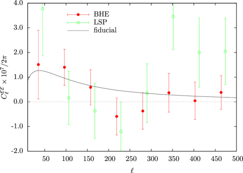
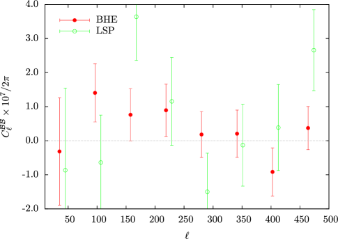
Figure 2: Left: The angular power spectrum for gradient modes obtained with the $\ell$-splitting method (LSP; green), compared with our fiducial method, based on Eq. (13) (BHE; red). The expected power spectrum with fiducial parameters from Dunkley:2010ge is shown as a black dashed line. Right: Same as right panel, but for curl mode.

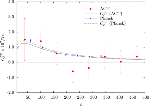
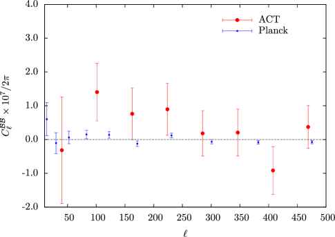
Figure 3: Left: Estimated angular power spectrum for gradient mode obtained from ACT (red) and Planck (blue), compared with the expected power spectrum with fiducial parameters from Ref. Dunkley:2010ge (ACT; black solid) and Ref. Ade:2013tyw (Planck; black dashed). Right: Same as right panel, but for curl mode.

Table 1: Comparison of parameter constraints on $\alpha^{\mathcal{E}}$ and $\alpha^{\mathcal{B}}$ with different methods and data.

	BHE	LSP	ACT Das:2011ak	Planck
$\alpha^{\mathcal{E}}$	$0.91\pm 0.46$	$1.06\pm 0.66$	$1.16\pm 0.29$	$0.94\pm 0.04$ Ade:2013tyw
$\alpha^{\mathcal{B}}$	$<0.80$	$<0.97$	$-$	$<0.014$

In this section, we show the angular power spectra of gradient and curl modes defined as

$$C_{L}^{\mathcal{E}\mathcal{E}}\equiv L^{4}C_{L}^{\phi\phi}\,,\qquad C_{L}^{\mathcal{B}\mathcal{B}}\equiv L^{4}C_{L}^{\varpi\varpi}\,.$$ (14)

To compare with Planck results, we compute the binned angular power spectra following the Planck analysis described in Ref. Ade:2013tyw . The details are shown in the following.

IV.1 Multipole binning

For gradient mode, to compute the binned angular power spectrum, we first estimate the amplitude of the lensing power spectrum defined as $\widehat{\alpha}^{\mathcal{E}}_{L}=\widehat{C}_{L}^{\mathcal{E}\mathcal{E}}/C_{L}^{\mathcal{E}\mathcal{E},\rm{fid}}$, where $\widehat{C}_{L}^{\mathcal{E}\mathcal{E}}$ and $C_{L}^{\mathcal{E}\mathcal{E},{\rm fid}}$ denote the measured and expected power spectra, respectively. The expected lensing power spectrum, $C_{L}^{\mathcal{E}\mathcal{E},{\rm fid}}$, is computed from the best-fit values of the temperature power spectrum from Dunkley:2010ge (Ade:2013zuv ) for ACT (Planck). Note that, by constraining $\widehat{\alpha}^{\mathcal{E}}_{L}$, we can show whether the measured lensing power spectrum is consistent with the lensing power spectrum expected from the flat $\Lambda$ cold dark matter framework. Then, the amplitude parameter at the $b$th multipole bin, $\widehat{\alpha}^{\mathcal{E}}_{b}$, is estimated as Ade:2013tyw

$$\widehat{\alpha}^{\mathcal{E}}_{b}\equiv(\sigma^{\mathcal{E}}_{b})^{2}\sum_{L^{b}_{\mathrm{min}}\leq L<L^{b}_{\mathrm{max}}}\mathscr{B}^{\mathcal{E}}_{L}\widehat{\alpha}^{\mathcal{E}}_{L}\,,$$ (15)

where $L^{b}_{\mathrm{min}}$ and $L^{b}_{\mathrm{max}}$ are the minimum and maximum multipoles of the $b$th bin, and the band-pass function and the variance of $\widehat{\alpha}^{\mathcal{E}}_{b}$ for the $b$th bin are given by

$$\mathscr{B}^{\mathcal{E}}_{L}=\left(\frac{C_{L}^{\mathcal{E}\mathcal{E},{\rm fid}}}{\Delta C_{L}^{\mathcal{E}\mathcal{E}}}\right)^{2}\,,\qquad\sigma^{\mathcal{E}}_{b}=\left\{\sum_{L}\mathscr{B}^{\mathcal{E}}_{L}\right\}^{-1/2}\,.$$ (16)

The error on angular power spectrum, $\Delta C_{L}^{\mathcal{E}\mathcal{E}}$ [and also $\Delta C_{L}^{\mathcal{B}\mathcal{B}}$ appearing later in Eq. (18)], is estimated from Eqs. (30) and (31) in Appendix A, respectively, for the bias-hardened estimator and $\ell$-splitting methods. The method to estimate the map-combined power spectrum is also described in Appendix A. For binning in multipoles, we choose $L^{b}_{\mathrm{min}}=10+(b-1)\times 490/n$ and $L^{b}_{\mathrm{max}}=10+b\times 490/n$, where the number of multipole bins is $n=8$. The measured power spectrum in the $b$th mulipole bin is then obtained by scaling $\widehat{\alpha}^{\mathcal{E}}_{b}$ with the expected power spectrum as

$$\widehat{C}^{\mathcal{E}\mathcal{E}}_{b}\equiv\widehat{\alpha}^{\mathcal{E}}_{b}C^{\mathcal{E}\mathcal{E},{\rm fid}}_{L_{b}}\,,$$ (17)

with $L_{b}=(L^{b}_{\mathrm{min}}+L^{b}_{\mathrm{max}})/2$. The error bars are also multiplied by $C^{\mathcal{E}\mathcal{E},{\rm fid}}_{L_{b}}$. On the other hand, for the curl modes, we compute the measured power spectrum in the $b$th bin as

$$\widehat{C}^{\mathcal{B}\mathcal{B}}_{b}\equiv(\sigma^{\mathcal{B}}_{b})^{2}\sum_{L^{b}_{\mathrm{min}}\leq L<L^{b}_{\mathrm{max}}}\frac{1}{(\Delta C_{L}^{\mathcal{B}\mathcal{B}})^{2}}\widehat{C}^{\mathcal{B}\mathcal{B}}_{L}\,,$$ (18)

where $\sigma^{\mathcal{B}}_{b}=[\sum_{L}(\Delta C_{L}^{\mathcal{B}\mathcal{B}})^{-2}]^{-1/2}$.

IV.2 Statistical analysis

Let us first discuss whether our measured gradient and curl modes are statistically consistent with other results. Provided $\widehat{\alpha}^{\mathcal{E}}_{b}$, the total lensing amplitude, $\alpha^{\mathcal{E}}$, is estimated by minimizing

$$-2\ln\mathcal{L}(\alpha^{\mathcal{E}})=\sum_{b=1}^{n}\frac{(\widehat{\alpha}^{\mathcal{E}}_{b}-\alpha^{\mathcal{E}})^{2}}{(\sigma^{\mathcal{E}}_{b})^{2}}\,.$$ (19)

The lensing power spectrum is estimated from both the BHE and LSP. The temperature multipoles with $500\leq\ell\leq 2000$ are used for BHE, and with the two disjoint annuli, $500\leq\ell\leq 1500$ and $1600\leq\ell\leq 2300$, for LSP. For curl mode, we estimate a parameter, $\alpha^{\mathcal{B}}$, by minimizing the following likelihood:

$$-2\ln\mathcal{L}(\alpha^{\mathcal{B}})=\sum_{b=1}^{n}\frac{(\widehat{C}^{\mathcal{B}\mathcal{B}}_{b}-\alpha^{\mathcal{B}}C^{\mathcal{B}\mathcal{B},{\rm fid}}_{b})^{2}}{(\sigma^{\mathcal{B}}_{b})^{2}}\,,$$ (20)

where the fiducial binned power spectrum, $C^{\mathcal{B}\mathcal{B},{\rm fid}}_{b}$, is computed with the same binning as the measured power spectrum, using the theoretical power spectrum with $G\mu=1.3\times 10^{-9}$ and $P=4.5\times 10^{-6}$ which is chosen so that the resultant $1\sigma$ upper bound on $\alpha^{\mathcal{B}}$ with ACT data roughly becomes unity.

Now we show the results of constraints on $\alpha^{\mathcal{E}}$ and $\alpha^{\mathcal{B}}$, which are summarized in Table 1. For the gradient mode, with our measured power spectrum from ACT, the constraint on parameter $\alpha^{\mathcal{E}}$ becomes $\alpha^{\mathcal{E}}=0.91\pm 0.46$ ($1\sigma$, BHE) and $\alpha^{\mathcal{E}}=1.06\pm 0.66$ ($1\sigma$, LSP),which is consistent with the Planck result within $1\sigma$ statistical significance, i.e., $\alpha^{\mathcal{E}}=0.943\pm 0.040$ ($1\sigma$). Our result is also consistent with $\alpha^{\mathcal{E}}=1.16\pm 0.29$ ($1\sigma$) obtained from the ACT map with noise level $\simeq 23\,\mu$K presented in Ref. Das:2011ak . Note that the degradation of statistical significance of our $\alpha^{\mathcal{E}}$ constraint compared to Ref. Das:2011ak would be due to the noise level and the use of the estimator, Eq. (7), for reducing mean-field bias.

On the other hand, for curl mode, we find $\alpha^{\mathcal{B}}<0.80$ ($1\sigma$, BHE) and $\alpha^{\mathcal{B}}<0.97$ ($1\sigma$, LSP) for our measured curl mode from ACT, and $\alpha^{\mathcal{B}}<0.014$ $(1\sigma)$ for Planck curl mode. Our analysis shows that we only obtain the upper bound for curl mode, and the curl mode is consistent with zero. For ACT data, further discussions on several systematics are given in Appendix B.

IV.3 Binned angular power spectra

In Fig. 2, we show the measured power spectrum for gradient (left) and curl modes (right) obtained by both BHE and LSP. For gradient modes, the measured power spectrum is compared with $C_{L}^{\mathcal{E}\mathcal{E},{\rm fid}}$. The mean of the measured power spectrum at several bins has a discrepancy with significance greater than $1\sigma$ level between the cases with BHE and LSP, both for gradient and curl modes. There are several possible systematics which would cause the discrepancy in our analysis; if there exist some additional sources of generating non-Gaussianity in the observed anisotropies, the normalization $A_{L}$ given in Eq. (10) which is derived in an idealistic case would lead to some amount of bias in the lensing estimator. The estimation of statistical error of the lensing power spectrum is also affected by the incorrect normalization, and underestimation of statistical errors in each bin causes the statistical discrepancy at each multipole bin. Moreover, the discrepancy is also caused by the systematics on LSP, in which we assume that the temperature multipoles on the two disjoint annuli are correlated solely due to the lensing effect. Nevertheless, the estimated total lensing amplitudes, $\alpha^{\mathcal{E}}$ and $\alpha^{\mathcal{B}}$, obtained from two different methods are consistent within $1\sigma$ level. In Appendix B, we also check the robustness of our analysis by changing multipole ranges, number of bins and size of multipole bins, and we confirm that the constraints on $\alpha^{\mathcal{E}}$ and $\alpha^{\mathcal{B}}$ obtained from these analyses are not so different from the constraints shown in Sec. IV.2. Since the amplitude of the string-induced curl-mode power spectrum is determined by the combination of $G\mu$ and $P$, the constraints on $G\mu$ and $P$ are almost determined by the constraints on the amplitude of curl-mode power spectrum, $\alpha^{\mathcal{B}}$. Thus, we expect that the impact of the residual systematics in the curl-mode power spectrum is not so significant on the final results of the parameter constraints. The statistical consistency between BHE and LSP would also indicate that the uncertainties in the subtraction of Gaussian bias and the contamination of N1 bias are also negligible. In the subsequent analysis, we use the BHE to constrain the string parameters.

In Fig. 3, the comparison of lensing power spectra obtained from ACT and Planck are shown. For gradient modes, the measured power spectrum agrees well with that obtained from Planck, and has a similar trend of multipole dependence. The resultant estimates of $\alpha^{\mathcal{E}}$ are also consistent with each other within $1\sigma$ level. For curl modes, although the multipole binning is different between Planck and our results, the resultant constraints on $\alpha^{\mathcal{B}}$ obtained from our results and Planck are consistent.

Before closing this section, we comment on the systematic effect of foreground contaminations on the curl-mode estimation. As mentioned in Ref. Das:2011ak , the lensing reconstruction with temperature maps around 148 GHz suffers from the foregrounds such as IR point sources and the Sunyaev-Zel’dovich (SZ) effect. Following Ref. Das:2011ak , we filter out the temperature multipoles below $500$ to mitigate atmospheric effect, and $\ell\raise 2.9pt\hbox{$\scriptstyle>$}\lower 0.5pt\hbox{$\scriptscriptstyle\sim$}\;2000$ to avoid foreground point sources. In the analysis of Planck Ade:2013aro , they use the temperature multipoles up to $\ell=1700$, and compare the resultant curl-mode power spectrum from 143 GHz with that from 217 GHz. In the above, we find that the resultant constraints on $\alpha^{\mathcal{B}}$ are both consistent with zero for Planck and ACT. Since the constraints on string parameters basically come from those on $\alpha^{\mathcal{B}}$, we expect that the residual foreground contaminations and the systematics in the Gaussian bias subtraction will not seriously affect the constraints on cosmic string parameters in both Planck and ACT cases.

V Constraints on cosmic string parameters

Figure 4: Constraints on string parameters, $P$ and $G\mu$, with the measured curl-mode power spectra. The colored regions are excluded with $>3\sigma$, $>2\sigma$ and $>1\sigma$ statistical significance with the curl mode from Planck (blue colored) and ACT (green colored). The black dashed line shows the lower bound of the string parameters disfavored by the temperature angular power spectrum Yamauchi:2010ms .

Now let us show the constraints on cosmic string parameters, i.e., string tension $G\mu$ and reconnection probability $P$, based on the measured curl-mode power spectrum obtained with the BHE. We compute the likelihood on the two-dimensional parameter space, $G\mu$ and $P$, given by

$$-2\ln\mathcal{L}(G\mu,P)=\sum_{b=1}^{n}\frac{(\widehat{C}^{\mathcal{B}\mathcal{B}}_{b}-C^{\mathcal{B}\mathcal{B},{\rm theo}}_{b}(G\mu,P))^{2}}{(\sigma^{\mathcal{B}}_{b})^{2}}\,,$$ (21)

where the quantity, $C^{\mathcal{B}\mathcal{B},{\rm theo}}_{b}(G\mu,P)$, is the theoretical binned power spectrum computed with specific values of $G\mu$ and $P$, with the same binning as shown in the measured power spectrum.

First, we focus on the ordinary field-theoretic strings with $P=1$. Assuming $P=1$ , we find the upper bound of the string tension from the curl-mode power spectrum from ACT and Planck as

$$G\mu\leq 8.9\times 10^{-4}\ \ (\,2\sigma\,,P=1\,,{\rm ACT}\,)\,,$$ (22)

$$G\mu\leq 6.6\times 10^{-5}\ \ (\,2\sigma\,,P=1\,,{\rm Planck}\,)\,,$$ (23)

respectively. These are rather weaker constraints than those obtained from temperature anisotropies through the GKS effect Dunkley:2010ge ; Ade:2013xla . On the other hand, for small values of $P$, the constraint on $G\mu$ from curl modes becomes tighter compared to that from the GKS effect. In Fig. 4, the resultant likelihood contours are shown for ACT (green colored) and Planck (blue colored), respectively. As we stated in Sec. II, the curl mode gives constraints on the combination of the string parameters as $G\mu P^{-1}$. Using ACT curl-mode data, we obtain constraints on the combination as

$$G\mu P^{-1}\leq 3.2\times 10^{-4}\ \ (\,2\sigma\,,{\rm ACT}\,)\,,$$ (24)

with $P\raise 2.9pt\hbox{$\scriptstyle<$}\lower 0.5pt\hbox{$\scriptscriptstyle\sim$}\;10^{-2}$. For Planck data this can be improved to

$$G\mu P^{-1}\leq 3.4\times 10^{-5}\ \ (\,2\sigma\,,{\rm Planck}\,)\,.$$ (25)

For comparison, the black solid line in Fig. 4 represents the lower bound of the string parameters disfavored by the temperature power spectrum Yamauchi:2010ms . For $P\raise 2.9pt\hbox{$\scriptstyle<$}\lower 0.5pt\hbox{$\scriptscriptstyle\sim$}\;10^{-4}$ ( $P\raise 2.9pt\hbox{$\scriptstyle<$}\lower 0.5pt\hbox{$\scriptscriptstyle\sim$}\;5\times 10^{-6}$ ), the constraint using the curl-mode power spectrum from Planck (ACT) is tighter than that from the GKS-induced temperature power spectrum. The curl mode is also useful in terms of robust constraints on cosmic strings, because the constraints from the GKS effect rely entirely on the measurement of the temperature power spectrum at small scales where the contributions from other secondary effects such as point sources and the SZ effect are usually significant. Note that the curl-mode power spectrum has been also measured from the South Pole Telescope temperature map vanEngelen:2012va , and compared to the ACT data, it gives a higher statistical significance on small scales. However, we expect that the constraints on $G\mu$ and $P$ from SPT are not dramatically improved so much, since these constraints mainly come from the lower-multipole power, for which we do not find any big difference between the ACT and SPT data.

Note that the error bars for ACT are estimated in an idealistic case, and the parameter constraints here may be underestimated. Even in this case, if the constraints were inflated by a factor of 2, the uncertainties in the model of cosmic strings would still be large. Our primary purpose is to show an example of cosmological application of curl mode. In this sense, although the constraints obtained here may be degraded, the curl mode is still useful to constrain cosmic strings.

VI Summary and future prospects

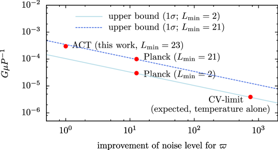
Figure 5: The $1\sigma$ constraints on the combination of cosmic string parameters, $G\mu P^{-1}$, as a function of improvement factor for the signal-to-noise ratio of curl mode normalized by the ACT case. For Planck, since the parameter constraint highly depends on the minimum value of curl mode multipoles for parameter constraints, $L_{\mathrm{min}}$, we also show the case with $L_{\mathrm{min}}=21$. The two lines show the expected upper bound on $G\mu P^{-1}$, with $L_{\mathrm{min}}=2$ (solid) or $L_{\mathrm{min}}=21$ (dashed), respectively. For comparison, we also show the case with cosmic-variance limit (CV-limit) with $L_{\mathrm{min}}=2$, where we assume that the temperature multipoles up to $\ell=7000$ are used for lensing reconstruction.

In this paper, we have presented constraints on cosmic strings with the curl-mode power spectrum from ACT and Planck. We first show the gradient and curl mode measured from ACT temperature map, and show that both the parameters, $\alpha^{\mathcal{E}}$ and $\alpha^{\mathcal{B}}$, are consistent between different methods and with other data within $1\sigma$ statistical significance, implying that residual systematics should be negligible in the resultant constraints on cosmic string parameters. Based on the measured curl-mode from ACT and Planck, we then obtain constraints on $P$ and $G\mu$. Although, for $P=1$, the constraint on $G\mu$ is weaker compared to the current constraint from the temperature power spectrum, we found that the constraints on the string parameters with the reconnection probability $P\raise 2.9pt\hbox{$\scriptstyle<$}\lower 0.5pt\hbox{$\scriptscriptstyle\sim$}\;10^{-4}$ become tighter than those from the temperature power spectrum via the GKS effect. With Planck data, we obtained an upper bound on the combination of the string parameters as $G\mu P^{-1}\raise 2.9pt\hbox{$\scriptstyle<$}\lower 0.5pt\hbox{$\scriptscriptstyle\sim$}\;3.4\times 10^{-5}$ with $P\raise 2.9pt\hbox{$\scriptstyle<$}\lower 0.5pt\hbox{$\scriptscriptstyle\sim$}\;10^{-2}$.

Note here that measurement of the curl-mode power spectrum can provide stringent constraints on the properties of the cosmic superstring network with an extremely small value of $P$. For instance, it is interesting to investigate a hybrid network model that contains bound states, in which strings with various values of the reconnection probability can be formed. The resultant curl-mode power spectrum generated from such network would be not so different from that used in this paper, and the qualitative constraints on a hybrid network could be also similar to those obtained in our analysis. The complete derivation of the curl-mode power spectrum from such network model is interesting, and we hope to come back to this issue in a future publication.

We now turn to discuss how the constraint on cosmic string parameters will be improved by the quality of curl-mode measurements. In Fig. 5, we show the constraint on $G\mu P^{-1}$ as a function of the improvement factor of the noise level of curl mode. Here we assume that only temperature maps are used for lensing reconstruction. For the Planck case, we also show results with the minimum value of curl-mode multipoles as $L_{\mathrm{min}}=21$. The result implies that, a measurement of lower multipoles of the curl-mode power spectrum is essential to constrain the string parameters. We also show the expected upper bound on $G\mu P^{-1}$ as a function of the improvement factor, extrapolated from the Planck results, in the case with $L_{\mathrm{min}}=2$ (solid line) and $L_{\mathrm{min}}=21$ (dashed line). Fig. 5, apparently indicates that the case of cosmic variance limit is not so improved compared to that of Planck. This implication, however, does not limit the potential of curl mode for constraining a model of cosmic string and/or other vector and tensor sources. In near future, several ground-based CMB experiments will focus on a precise measurement of B-mode polarization. In the case of the cosmic-variance limit, the inclusion of polarization improves the signal-to-noise ratio of curl mode by $2$ orders of magnitude compared to the case without polarization Namikawa:2011cs . This leads to an expected constraint on $G\mu P^{-1}$ of $\sim 5\times 10^{-7}$. Moreover, as shown in Ref. Hirata:2003ka , measurements of B-mode polarization on small scales directly probe the lensing potentials, and thus the Gaussian bias, in principle, vanishes in the absence of primordial B-mode polarizations and other non-lensing B-mode sources. Therefore, measurements of polarization anisotropies should eventually lead to a high-precision lensing reconstruction, and this can give a further improvement of constraints on cosmic string parameters.

Appendix A Error estimate of angular power spectrum

Table 2: Constraints on $\alpha^{\mathcal{E}}$ while varying the maximum value of temperature multipoles used for lensing reconstruction, $\ell_{\mathrm{max}}$.

$\ell_{\mathrm{max}}$	$1900$	$2000$	$2100$
$\alpha^{\mathcal{E}}$	$1.00\pm 0.51$	$0.91\pm 0.46$	$0.88\pm 0.44$
$\alpha^{\mathcal{B}}$	$<0.91$	$<0.80$	$<0.79$

Table 3: Same as Table 2, but for a varying number of lensing multipoles bins, $n$.

Number of bins	$7$	$8$	$9$
$\alpha^{\mathcal{E}}$	$0.91\pm 0.46$	$0.91\pm 0.46$	$0.91\pm 0.46$
$\alpha^{\mathcal{B}}$	$<0.81$	$<0.80$	$<0.86$

Table 4: Same as Table 2, but for comparing with the results obtained by $\ell$-splitting. The multipole range of $\ell$-splitting is varied as $([500,1500],[1600,2300])$ (LSP), $([500,1550],[1600,2300])$ (LSP^′), $([500,1500],[1550,2300])$ (LSP^′′) .

Method	BHE	LSP	LSP′	LSP′′
$\alpha^{\mathcal{E}}$	$0.91\pm 0.46$	$1.06\pm 0.66$	$1.01\pm 0.63$	$1.26\pm 0.66$
$\alpha^{\mathcal{B}}$	$<0.80$	$<0.97$	$<0.98$	$<0.93$

A.1 Expected error estimate

For the $i$th map, given Fourier multipoles, $X_{\bm{L}}$, the optimal unbiased estimator for the angular power spectrum is given by

$$\widehat{C}^{XX}_{L}=\frac{1}{WN_{L}}\sum_{|\bm{L}|=L}|X_{\bm{L}}|^{2}\,,$$ (26)

where $N_{L}$ is the number of fluctuations whose multipole coefficient satisfies $|\bm{L}|=L$, and we assume

$$\langle X_{\bm{L}}X_{\bm{L}^{\prime}}\rangle=WC^{XX}_{L}\delta_{\bm{L}-\bm{L}^{\prime}}\,.$$ (27)

The normalization, $W$, is usually arising from, e.g., the effect of a window function. The error is then estimated as

$$[\Delta C_{L}^{XX}]^{2} =\frac{1}{N_{L}^{2}}\sum_{|\bm{L}|=L}\sum_{|\bm{L}^{\prime}|=L}\frac{\langle|X_{\bm{L}}|^{2}|X_{\bm{L}^{\prime}}|^{2}\rangle}{W^{2}}-(C^{XX}_{L})^{2}$$

$$=\frac{1}{N_{L}^{2}}\sum_{|\bm{L}|=L}\frac{2(WC_{L}^{XX})^{2}}{W^{2}}$$

$$=\frac{2}{N_{L}}(C_{L}^{XX})^{2}\,,$$ (28)

where we assume $X_{\bm{L}}$ is a random Gaussian field. We will use the above expression for the error estimate.

A.2 Map-combined power spectrum

In our analysis, the angular power spectra, $C_{L}^{\mathcal{E}\mathcal{E}}$ and $C_{L}^{\mathcal{B}\mathcal{B}}$, are first estimated in each map based on Eq. (12). The map-combined power spectrum is then obtained by weighting the inverse of its variance (e.g., vanEngelen:2012va ):

$$\widehat{C}^{XX}_{L}=\left\{\sum_{i}\frac{1}{[\Delta C^{XX}_{L,i}]^{2}}\right\}^{-1}\sum_{i}\frac{\widehat{C}^{XX}_{L,i}}{[\Delta C^{XX}_{L,i}]^{2}}\,,$$ (29)

where $X=\mathcal{E}$ or $\mathcal{B}$, and the variance of the angular power spectrum in each map is estimated with the ideal case based on Eq. (28):

$$[\Delta C_{L,i}^{XX}]^{2} =\frac{2}{N_{L}}(\mathcal{A}_{L,i}^{XX}+C_{L}^{XX})^{2}\,,$$ (30)

with $\mathcal{A}_{L,i}^{XX}$ denoting the normalization (9) for the $i$th map, and $N_{L}$ being the number of fluctuations whose multipole coefficient satisfies $|\bm{L}|=L$. For $\ell$-splitting, instead of Eq. (30), we estimate the error of the measured power spectrum as

$$[\Delta C_{L,i}^{XX}]^{2}=\frac{1}{N_{L}}(\mathcal{A}_{L,i}^{XX,(1)}+C_{L}^{XX,{\rm fid}})(\mathcal{A}_{L,i}^{XX,(2)}+C_{L}^{XX,{\rm fid}})\,,$$ (31)

where the quantities, $\mathcal{A}_{L,i}^{XX,(1)}$ and $\mathcal{A}_{L,i}^{XX,(2)}$, are the normalization computed on each disjoint annulus.

Appendix B Test for systematic uncertainties

In this section, we show several tests for systematic uncertainties in estimating lensing power spectra.

B.0.1 Temperature multipoles, $\ell_{\mathrm{min}}$ and $\ell_{\mathrm{max}}$

Here we show the dependence of our results on the range of temperature multipoles. The results of parameter constraints on $\alpha^{\mathcal{E}}$ and $\alpha^{\mathcal{B}}$ are given in Table 2.

B.0.2 Binning of measured power spectrum

To test whether or not our results depend on the binning of measured lensing power spectra, we compute the constraints on $\alpha^{\mathcal{E}}$ and $\alpha^{\mathcal{B}}$, while varying the number of multipole bins, $n$. In Table 3, to compare with our fiducial number of bins, $n=8$, we show $n=8\pm 1$ cases.

B.0.3 Method of lensing reconstruction

To test the effect of these biases, we compare with the results of lensing reconstruction with the $\ell$-splitting method. In Table 4, we show the results of constraints on $\alpha^{\mathcal{E}}$ and $\alpha^{\mathcal{B}}$, while varying several cases of two disjoint annuli.

References

- (1) K. M. Smith, O. Zahn, and O. Dore, “Detection of Gravitational Lensing in the Cosmic Microwave Background”, Phys. Rev. D 76 (2007) 043510, [arXiv:0705.3980].
- (2) C. M. Hirata, S. Ho, N. Padmanabhan, U. Seljak, and N. A. Bahcall, “Correlation of CMB with large-scale structure: II. Weak lensing”, Phys. Rev. D78 (2008) 043520, [arXiv:0801.0644].
- (3) S. Das, B. D. Shewin, et al., “Detection of the Power Spectrum of Cosmic Microwave Background Lensing by the Atacama Cosmology Telescope”, Phys. Rev. Lett. 107 (2011) 021301, [arXiv:1103.2124].
- (4) A. van Engelen, R. Keisler, O. Zahn, K. Aird, B. Benson, et al., “A measurement of gravitational lensing of the microwave background using South Pole Telescope data”, Astrophys.J. 756 (2012) 142, [arXiv:1202.0546].
- (5) L. Bleem, A. van Engelen, G. Holder, et al., “A Measurement of the Correlation of Galaxy Surveys with CMB Lensing Convergence Maps from the South Pole Telescope”, Astrophys. J. 753 (2012) L9, [arXiv:1203.4808].
- (6) B. D. Sherwin, S. Das, A. Hajian, et al., “The Atacama Cosmology Telescope: Cross-Correlation of CMB Lensing and Quasars”, Phys.Rev. D86 (2012) 083006, [arXiv:1207.4543].
- (7) S. Das, T. Louis, M. R. Nolta, et al., “The Atacama Cosmology Telescope: Temperature and Gravitational Lensing Power Spectrum Measurements from Three Seasons of Data”, arXiv:1301.1037.
- (8) Planck Collaboration, “Planck 2013 results. XVII. Gravitational lensing by large-scale structure”, arXiv:1303.5077.
- (9) Planck Collaboration, “Planck 2013 results. XVIII. Gravitational lensing-infrared background correlation”, arXiv:1303.5078.
- (10) D. Hanson, S. Hoover, A. Crites, et al., “Detection of B-mode Polarization in the Cosmic Microwave Background with Data from the South Pole Telescope”, Phys. Rev. Lett. 111 (2013) 141301, [arXiv:1307.5830].
- (11) Planck Collaboration, “The scientific programme”, astro-ph/0604069.
- (12) L. Bleem, M. Lueker, S. Padin, E. Shirokoff, and J. Vieira, “An Overview of the SPTpol Experiment”, Journal of Low Temperature Physics (2012) 859–864.
- (13) POLARBEAR Collaboration, “The new generation CMB B-mode polarization experiment: POLARBEAR”, arXiv:1011.0763.
- (14) M. Niemack, P. Ade, J. Aguirre, F. Barrientos, J. Beall, et al., “ACTPol: A polarization-sensitive receiver for the Atacama Cosmology Telescope”, Proc.SPIE Int.Soc.Opt.Eng. 7741 (2010) 77411S, [arXiv:1006.5049].
- (15) COrE Collaboration, “COrE (Cosmic Origins Explorer) A White Paper”, arXiv:1102.2181.
- (16) PRISM Collaboration, “PRISM (Polarized Radiation Imaging and Spectroscopy Mission): A White Paper on the Ultimate Polarimetric Spectro-Imaging of the Microwave and Far-Infrared Sky”, arXiv:1306.2259.
- (17) K. M. Smith et al., “CMBPol Mission Concept Study: Gravitational Lensing”, AIP Conf.Proc. 1141 (2009) 121, [arXiv:0811.3916].
- (18) W. Hu, “Dark Synergy: Gravitational Lensing and the CMB”, Phys. Rev. D65 (2002) 023003, [astro-ph/0108090].
- (19) J. Lesgourgues and S. Pastor, “Massive neutrinos and cosmology”, Phys. Rep. 429 (2006) 307–379, [astro-ph/0603494].
- (20) R. de Putter, O. Zahn, and E. V. Linder, “CMB Lensing Constraints on Neutrinos and Dark Energy”, Phys. Rev. D 79 (2009) 065033, [arXiv:0901.0916].
- (21) T. Namikawa, S. Saito, and A. Taruya, “Probing dark energy and neutrino mass from upcoming lensing experiments of CMB and galaxies”, JCAP 1012 (2010) 027, [arXiv:1009.3204].
- (22) S. Das, R. de Putter, E. V. Linder, and R. Nakajima, “Weak Lensing Science, Surveys, and Systematics”, JCAP 1211 (2012) 011, [arXiv:1102.5090].
- (23) C. M. Hirata and U. Seljak, “Reconstruction of lensing from the cosmic microwave background polarization”, Phys. Rev. D68 (2003) 083002, [astro-ph/0306354].
- (24) A. Cooray, M. Kamionkowski, and R. R. Caldwell, “Cosmic shear of the microwave background: The curl diagnostic”, Phys. Rev. D 71 (2005) 123527, [astro-ph/0503002].
- (25) T. Namikawa, D. Yamauchi, and A. Taruya, “Full-sky lensing reconstruction of gradient and curl modes from CMB maps”, JCAP 1201 (2012) 007, [arXiv:1110.1718].
- (26) E. J. Copeland, R. C. Myers, and J. Polchinski, “Cosmic F- and D-strings”, JHEP 06 (2004) 013, [hep-th/0312067].
- (27) M. G. Jackson, N. T. Jones, and J. Polchinski, “Collisions of cosmic F- and D-strings”, JHEP 10 (2005) 013, [hep-th/0405229].
- (28) D. Yamauchi, T. Namikawa, and A. Taruya, “Weak lensing generated by vector perturbations and detectability of cosmic strings”, JCAP 1210 (2012) 030, [arXiv:1205.2139].
- (29) D. Yamauchi, T. Namikawa, and A. Taruya, “Full-sky formulae for weak lensing power spectra from total angular momentum method”, JCAP 1308 (2013) 051, [arXiv:1305.3348].
- (30) N. Kaiser and A. Stebbins, “Microwave anisotropy due to cosmic strings”, Nature 310 (1984) 391–393.
- (31) J. R. Gott, “Gravitational lensing effects of vacuum strings - Exact solutions”, Astrophys. J. 288 (1985) 422.
- (32) D. Yamauchi, T. Namikawa, and A. Taruya, “in prep”, .
- (33) D. B. Thomas, C. R. Contaldi, and J. Magueijo, “Rotation of galaxies as a signature of cosmic strings in weak lensing surveys”, Phys.Rev.Lett. 103 (2009) 181301, [arXiv:0909.2866].
- (34) C. J. A. P. Martins and E. P. S. Shellard, “Quantitative String Evolution”, Phys. Rev. D54 (1996) 2535–2556, [hep-ph/9602271].
- (35) C. J. A. P. Martins and E. P. S. Shellard, “Extending the velocity-dependent one-scale string evolution model”, Phys. Rev. D65 (2002) 043514, [hep-ph/0003298].
- (36) A. Avgoustidis and E. P. S. Shellard, “Effect of Reconnection Probability on Cosmic (Super)string Network Density”, Phys. Rev. D 73 (2006) 041301, [astro-ph/0512582].
- (37) K. Takahashi, A. Naruko, Y. Sendouda, D. Yamauchi, C.-M. Yoo, and M. Sasaki, “Non-Gaussianity in Cosmic Microwave Background Temperature Fluctuations from Cosmic (Super-)Strings”, JCAP 0910 (2009) 003, [arXiv:0811.4698].
- (38) D. Yamauchi, K. Takahashi, Y. Sendouda, C.-M. Yoo, and M. Sasaki, “Analytical model for CMB temperature angular power spectrum from cosmic (super-)strings”, Phys. Rev. D82 (2010) 063518, [arXiv:1006.0687].
- (39) D. Yamauchi, Y. Sendouda, C.-M. Yoo, K. Takahashi, A. Naruko, and M. Sasaki, “Skewness in CMB temperature fluctuations from curved cosmic (super-)strings”, JCAP 1005 (2010) 033, [arXiv:1004.0600].
- (40) http://lambda.gsfc.nasa.gov/.
- (41) R. Dunner, M. Hasselfield, T. A. Marriage, J. Sievers, et al., “The Atacama Cosmology Telescope: Data Characterization and Map Making”, Astrophys. J. 762 (2013) 10, [arXiv:1208.0050].
- (42) T. Namikawa, D. Hanson, and R. Takahashi, “Bias-Hardened CMB Lensing”, Mon. Not. Roy. Astron. Soc. 431 (2013) 609–620, [arXiv:1209.0091].
- (43) M. Zaldarriaga and U. Seljak, “Reconstructing projected matter density from cosmic microwave background”, Phys. Rev. D59 (1999) 123507, [astro-ph/9810257].
- (44) W. Hu and T. Okamoto, “Mass Reconstruction with CMB Polarization”, Astrophys. J. 574 (2002) 566–574, [astro-ph/0111606].
- (45) A. Lewis, A. Challinor, and A. Lasenby, “Efficient Computation of CMB anisotropies in closed FRW models”, Astrophys. J. 538 (2000) 473–476, [astro-ph/9911177].
- (46) J. Dunkley, R. Hlozek, J. Sievers, et al., “The Atacama Cosmology Telescope: Cosmological Parameters from the 2008 Power Spectra”, Astrophys. J. 739 (2011) 53, [arXiv:1009.0866].
- (47) M. H. Kesden, A. Cooray, and M. Kamionkowski, “Lensing Reconstruction with CMB Temperature and Polarization”, Phys. Rev. D67 (2003) 123507, [astro-ph/0302536].
- (48) A. Benoit-Levy, T. Dechelette, K. Benabed, J.-F. Cardoso, D. Hanson, and S. Prunet, “Full-sky CMB lensing reconstruction in presence of sky-cuts”, Astronomy & Astrophysics 555 (2013) 10, [arXiv:1301.4145].
- (49) W. Hu, “Angular trispectrum of the CMB”, Phys. Rev. D64 (2001) 083005, [astro-ph/0105117].
- (50) B. D. Sherwin and S. Das, “CMB Lensing - Power Without Bias”, arXiv:1011.4510.
- (51) T. Okamoto and W. Hu, “CMB Lensing Reconstruction on the Full Sky”, Phys. Rev. D67 (2003) 083002, [astro-ph/0301031].
- (52) Planck Collaboration, “Planck 2013 results. XVI. Cosmological parameters”, arXiv:1303.5076.
- (53) Planck Collaboration, “Planck 2013 results. XXV. Searches for cosmic strings and other topological defects”, arXiv:1303.5085.