Importance of complex orbitals in calculating the self-interaction corrected ground state of atoms

Abstract

The ground state of atoms from H to Ar was calculated using a self-interaction correction to local and gradient dependent density functionals. The correction can significantly improve the total energy and makes the orbital energies consistent with ionization energies. However, when the calculation is restricted to real orbitals, application of the self-interaction correction can give significantly higher total energy and worse results, as illustrated by the case of the Perdew-Burke-Ernzerhof gradient dependent functional. This illustrates the importance of using complex orbitals for systems described by orbital density dependent energy functionals.

Density functional theory (DFT) of electronic systems has become a widely used tool in calculations for solids, liquids, and molecules Koh99 . The most commonly used approximation to the exact energy functional for extended systems is the so-called generalized gradient approximation (GGA), where the functional only depends on the total spin density and its gradient, an improvement on the local density approximation (LDA), where gradients are not included. The kinetic energy is commonly evaluated by introducing orthonormal orbitals, $\varphi_{i}({\bf r})$, consistent with a given total electron density, $\rho({\bf r})=\sum_{i}|\varphi_{i}({\bf r})|^{2}$. In many cases, DFT significantly improves the total energy over the Hartree-Fock (HF) method and gives acceptable accuracy with smaller computational effort. However, a number of shortcomings are also known: The bond energy tends to be too large while the activation energy for atomic rearrangements tends to be underestimated Nac96 . There is also a tendency to over delocalize spin density, sometimes making localized electronic defects unstable with respect to delocalization Pac00 . For finite systems, an ionization energy (IE) can be determined as the energy difference between the ground states of charged and neutral species. These values often agree well with experiment, but ionization from deeper energy levels and ionization from solids cannot be estimated this way. Unlike in HF theory, the energy associated with the orbitals (single particle eigenvalues) is in practice neither a good nor a theoretically justified estimate of ionization energy. Even the exact DFT functional would give an estimate of only the first ionization energy.

A leading source of error is the spurious self-interaction introduced when the Hartree energy $E_{\text{H}}$ is evaluated from the total electron density $\rho({\bf r})$:

$$E_{\rm H}[\rho]=\frac{1}{2}\int\!d^{3}{\bf r}d^{3}{\bf r}^{\prime}\ \frac{\rho({\bf r})\rho({\bf r}^{\prime})}{|{\bf r}-{\bf r}^{\prime}|}$$ (1)

If the orbital densities $\rho_{i}({\bf r})=|\varphi_{i}({\bf r})|^{2}$ represent single particle distributions, a more accurate expression is

$$E^{\text{ODD}}_{\rm H}[\rho^{N}]=\frac{1}{2}\sum_{i\neq j}\int\!d^{3}{\bf r}d^{3}{\bf r}^{\prime}\ \frac{\rho_{i}({\bf r})\rho_{j}({\bf r}^{\prime})}{|{\bf r}-{\bf r}^{\prime}|}.$$ (2)

Here, $\rho^{N}$ denotes the set of orbital densities $\{\rho_{1},\dots,\rho_{N}\}$ corresponding to the set of occupied orbitals, $\{\varphi_{1},\dots,\varphi_{N}\}$, denoted by $\varphi^{N}$. This expression for the energy is explicitly orbital-density dependent (ODD). The difference between the two expressions is the diagonal terms ($i=j$), which can be interpreted as the interaction of the electron in each orbital with itself. In Hartree-Fock calculations, where the Hartree energy is evaluated as in Eq. (1), the exchange energy includes equally large self-interaction with opposite sign, so the self-interaction cancels out exactly. In LDA and GGA [collectively referred to as Kohn-Sham (KS) here], the exchange-correlation energy, $E_{\text{xc}}$, is approximate and the cancellation is incomplete. Perdew and Zunger Per81 proposed an orbital-based self-interaction correction (SIC)

$$E_{\text{SIC}}\left[\rho^{N}\right]=E_{\text{KS}}\left[\rho\right]-\sum_{i=1}^{N}E_{\text{SI}}\left[\rho_{i}\right]$$ (3)

using $E_{\text{SI}}\left[\rho_{i}\right]=E_{\text{H}}\left[\rho_{i}\right]+E_{\text{xc}}\left[\rho_{i}\right]$. Other estimates of SIC can be formulated Leg02andLun01 ; Vyd06 , but here we take Eq. (3) to be the definition. Originally, SIC was proposed for LDA, but it can in principle be applied to other functionals. These are examples of a more general class of functionals, ODD functionals, where the Hartree energy is evaluated from Eq. (2).

Variational optimization of orbital dependent functionals is typically carried out by adding the orthonormality constraints multiplied by Lagrange multipliers, $\lambda_{ji}$, to the energy functional to give

$$S\left[\rho^{N}\right]=E_{\text{SIC}}\left[\rho^{N}\right]-\sum_{i,j=1}^{N}\lambda_{ji}\left(\braket{\varphi_{i}}{\varphi_{j}}-\delta_{ij}\right)$$ (4)

and finding a stationary point with respect to variation of each orbital $|\varphi_{i}\rangle$ and its complex conjugate. This gives two sets of equations for the optimal orbitals Ped84and85 ; Sva96andGoe97 ; Mes08and09 ,

$$\widehat{H}_{i}|\varphi_{i}\rangle = \sum_{i=1}^{N}\lambda_{ji}|\varphi_{j}\rangle\quad{\rm and}\ \ \ \boldsymbol{\lambda}=\boldsymbol{\lambda}^{\dagger},$$ (5)

with $\widehat{H}_{i}|\varphi_{i}\rangle={\delta E_{\text{SIC}}}/{\delta\varphi_{i}}$ and $\lambda_{ji}=\braket{\varphi_{j}}{\widehat{H}_{i}}{\varphi_{i}}$. The ODD functional form leads to orbital-dependent Hamiltonians, $\widehat{H}_{i}$. In the case of SIC, $E_{\text{SI}}$ is the orbital density dependent part of the energy while $E_{\text{KS}}$ only depends on the total spin density, so that

$$\widehat{H}_{i}=\widehat{H}_{\text{KS}}[\rho]+{\hat{v}}[\rho_{i}]$$ (6)

where ${\hat{v}}[\rho_{i}]=-{\delta E_{\text{SI}}\left[\rho_{i}\right]}/{\delta\rho_{i}}=-({\hat{v}}_{\text{H}}[\rho_{i}]+{\hat{v}}_{\text{x}c}[\rho_{i}])$. At the minimum, the constraint matrix $\boldsymbol{\lambda}$ is Hermitian and can be diagonalized to give orbital energies $\varepsilon_{i}$ and corresponding eigenfunctions, the canonical orbitals, $\psi^{N}$. In terms of these, condition (5) can be written as

$$\widehat{H}|\psi_{i}\rangle=\varepsilon_{i}|\psi_{i}\rangle\ ,\quad\varepsilon_{i}\delta_{ij}=({\bf W}{\boldsymbol{\lambda}}{\bf W^{\dagger}})_{ij}$$ (7)

with $|\psi_{i}\rangle=\sum_{k=1}^{N}W_{ki}|\varphi_{k}\rangle$. The non-local operator $\widehat{H}$ is defined in terms of the $N$ optimal orbitals $\varphi^{N}$ and their corresponding Hamiltonians $\widehat{H}_{i}$. In this way, the single-particle equations (5) can be decoupled to give traditional eigenvalue equations Mes08and09 . The calculation is carried out using two sets of orbitals, $\varphi^{N}$ and $\psi^{N}$, while keeping track of the transformation matrix, ${\bf W}$, relating the two sets. In HF and KS-DFT, the energy is independent of the unitary transformation and the optimal orbitals are typically chosen to be the same as the canonical orbitals, i.e., ${\bf W}={\bf 1}$.

At intermediate steps of the variational optimization of ODD functionals, $\boldsymbol{\lambda}$ is in general not Hermitian, but can be made Hermitian by finding the unitary transformation that zeros the matrix $\boldsymbol{\kappa}=\boldsymbol{\lambda}-\boldsymbol{\lambda}^{\dagger}$ Ped84and85 , where

$$\kappa_{ij} = \int\!d^{3}{\bf r}\ \varphi^{*}_{i}({\bf r})\varphi_{j}({\bf r})\left(v[\rho_{i}]({\bf r})-v[\rho_{j}]({\bf r})\right)=0.$$ (8)

With a Hermitian $\boldsymbol{\lambda}$ at each iteration, Eq. (7) can be used during the minimization of the energy in a scheme analogous to what is done in KS-DFT and HF.

The results presented here were obtained with the program quantice quantice using the Cartesian representation of the Gaussian-type correlation-consistent polarized valence quadruple zeta (cc- pVQZ)Woo94 basis set and numerical grids of 75 radial shells of 302 points Mur96andLeb99 . The convergence criterion in the optimization was a squared residual norm below 10^-5 eV². For LDA, Slater exchange and the Perdew-Wang parameterization of correlation is used (SPW92)LDA .

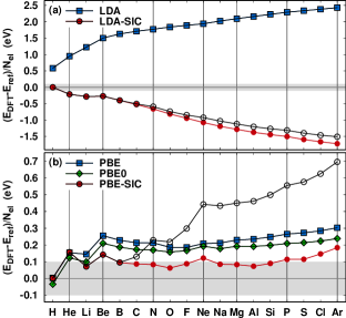
Figure 1: (Color online) Energy of atoms H to Ar using LDA, LDA-SIC, PBE, PBE-SIC, and PBE0 functionals compared with accurate, non-relativistic estimates Cha96 , normalized to the number of electrons. Results obtained with complex orbitals (solid symbols) and real orbitals (open symbols) are also compared. Vertical lines indicate the $s^{2}$, $p^{3}$, and $p^{6}$ electron configurations. The gray shading at $\pm$0.1 eV illustrates the different energy scales in (a) and (b). When complex orbitals are used, PBE-SIC gives significant improvement in the total energy, but not when real orbitals are used.

Figure 1 compares the energy of the atoms H to Ar, calculated using various functionals, with accurate reference values Cha96 . While the inclusion of gradients in the GGA type PBE functional Per96a improves on the results obtained with LDA, the energy is still significantly too high and the error per electron tends to increase with the size of the atom. SIC applied to LDA reduces the magnitude of the error but gives a strong overcorrection. The overcorrection also increases with the atomic number. When SIC is applied to the gradient-dependent PBE functional, the error is reduced to $\sim$0.1 eV per electron. But, this improvement is only obtained if the optimal orbitals are complex, i.e., complex linear combination coefficients are used for the expansion of the orbitals in the Gaussian basis. When real expansion coefficients are used, the SIC actually increases the error substantially, as had already been noted previously Vyd04 . A common approach to improve the results obtained with DFT is to mix in HF exchange with GGA and LDA in so called hybrid functionals Bec93a . The PBE0 PBE0 hybrid functional only gives slightly better results than PBE (see Fig. 1). PBE-SIC with complex orbitals gives more accurate total energy.

The ionization energy can be evaluated as the energy difference of the charged and neutral system. These values typically agree to within $\pm 5\%$ with experiment for the atoms H to Ar, both for PBE and PBE-SIC. However, in extended systems, subject to periodic boundaries, the charged system can not be calculated rigorously, so the IE has to be extracted from ground-state properties.

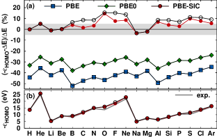
Figure 2: (Color online) (a) Comparison of the eigenvalue of the highest occupied orbital $\varepsilon_{\text{HOMO}}$ with $\Delta E=E_{\text{cation}}-E_{\text{neutral}}$. (b) Comparison of PBE-SIC eigenvalues with experimental ionization energy NIST . Open and solid symbols are used as in Fig. 1. PBE-SIC eigenvalues agree much better than PBE and PBE0 with both the calculated energy difference and experimental data.

In Fig. 2, the energy eigenvalue of the highest occupied canonical orbital is compared with the calculated IE using the functionals PBE, PBE0, and PBE-SIC. As is well known, for the commonly used LDA and GGA functionals, the eigenvalues obtained from KS-DFT do not give good estimates of ionization energy. The IE estimates from PBE and PBE0 eigenvalues are too low, with errors of $\sim$40% and 30% respectively. In PBE-SIC, however, the values are better, in most cases the error is within 5%-10%. The eigenvalues are also in good agreement with experimental data on IE NIST , as shown in Fig. 2. The values obtained from complex orbitals are closer to both experiment and the calculated energy difference than those obtained using real orbitals. A similar improvement is observed for ionization from lower lying orbitals. For argon, for example, the second, third, and fourth highest orbital energies in PBE-SIC using complex orbitals deviate by 5%, 3%, and 1% (1.5, 7, and -3 eV), respectively, from measured photoionization energy Shi77 . Real orbitals give similar deviations of 10%, 3%, and 1% (2.8, 7, and 2 eV), while the PBE values are off by 18%, 8%, and 10% (-5.2, -19, and -32 eV).

Figure 3 compares the PBE-SIC ground state for neon using real and complex orbitals. In both cases the canonical orbitals are of $s$ and $p$ type and the total density is spherical. The optimal orbitals, however, differ significantly in shape. The real orbitals are aligned in the traditional tetrahedral $sp^{3}$ configuration and can be constructed from the canonical orbitals as $\varphi_{r1}=\frac{1}{2}(s+p_{x}+p_{y}+p_{z})$ followed by three consecutive fourfold improper rotations about the $z$ axis, $\hat{S}_{4}(z)$. The complex optimal orbitals are also, despite their uncommon tetragonal configuration, sp³-hybrid orbitals. Such a set can be constructed from $\varphi_{c1}=\frac{1}{2}(s+p_{x}+p_{y}+{\rm i}\;p_{z})$ and application of the rotations $\hat{S}_{4}(z)$. The shape of a real and complex orbital is compared in Fig. 4. The density of the real orbital has axial symmetry and a nodal surface. The complex orbital has lower symmetry and lacks the nodal surface since orthogonality is achieved by the phase of the complex expansion coefficients.

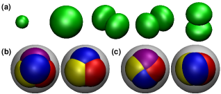
Figure 3: (Color online) Orbital densities of a Ne atom obtained from a PBE-SIC calculation. (a) Electron density isosurfaces of the complex canonical orbitals show clear correspondence with $s$ and $p$ orbitals. The real canonical orbitals have a similar shape. Electron density isosurfaces from (b) real and (c) complex optimal valence orbitals shown from the top and side views for one spin component. The gray spheres show the total density.

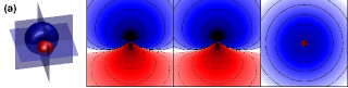
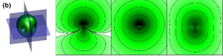
Figure 4: (Color online) Isosurface and contour plots of an optimal valence orbital of neon obtained with PBE-SIC using (a) real and (b) complex expansion coefficients. The contour plots show the orbital density in three planes through the nucleus. The complex orbital has lower symmetry and no nodal surface.

The large increase in total energy that occurs when the SIC calculation is restricted to real orbitals was also observed for other GGA-SIC functionals as well as for exchange-only SIC calculations. This effect can be explained by the fundamentally different structure of the functional as compared to KS or HF. There, the energy is invariant with respect to unitary transformations of the orbitals so the full flexibility of complex expansion coefficients is not needed. The SIC energy, however, depends explicitly on the orbital densities. Nodal surfaces, which are required for orthogonality of real orbitals, impose a strong constraint on the shape of the orbital densities (and their gradient, resulting in a stronger effect on the energy for SIC applied to GGA functionals Vyd06 ). This can be illustrated by a simple example: Given a basis set consisting of two Cartesian $p$-type orbitals,

$$\varphi^{c}_{1}({\bf r})=Nxe^{-\beta{\bf r}^{2}},\ \varphi^{c}_{2}({\bf r})=Nye^{-\beta{\bf r}^{2}},$$ (9a)

a second set can be constructed as the complex spherical representation,

$$\varphi^{s}_{1}({\bf r}) = \frac{N}{\sqrt{2}}\overline{r}e^{{\rm i}\phi}e^{-\beta{\bf r}^{2}},\ \varphi^{s}_{2}({\bf r})=\frac{N}{\sqrt{2}}\overline{r}e^{-{\rm i}\phi}e^{-\beta{\bf r}^{2}},$$ (9b)

where $\overline{r}=\sqrt{x^{2}+y^{2}}$. The two sets of orthogonal orbitals accessible by real linear combinations are defined by a single parameter $\alpha$:

$$\widetilde{\varphi}^{x}_{1} = \quad\cos(\alpha)\varphi^{x}_{1}+\sin(\alpha)\varphi^{x}_{2}$$ (10a)

$$\widetilde{\varphi}^{x}_{2} = -\sin(\alpha)\varphi^{x}_{1}+\cos(\alpha)\varphi^{x}_{2}\ ,\quad x\in\{c,s\}$$ (10b)

The orbital densities are illustrated in Fig. 5 for several values of $\alpha$. For the Cartesian basis (9a), the variation of $\alpha$ results in a rotation of the orbitals about the $z$ axis, while for the spherical basis a transition from delocalized to localized orbitals occurs. The SIC calculated from the Cartesian basis is independent of $\alpha$, but for the spherical basis the energy of the localized and delocalized orbitals will differ. While the spherical basis (9b) can produce delocalized orbitals, it is incapable of describing localized orbital densities pointing in the “diagonal” orientation if real linear combination coefficients are used. Only when complex coefficients are used, can both basis sets give the full range of possibilities.

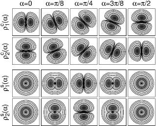
Figure 5: Orbital densities obtained from the Cartesian (upper panel) and spherical basis (lower panel) using real expansion coefficients. The Cartesian basis only gives localized orbitals but allows for all orientations. The spherical basis makes a transition from delocalized to localized orbitals possible but is restricted to certain orientations of the localized orbitals.

While errors in the total energy of atoms can, to a large extent, cancel out when the energy differences of two atomic configurations are calculated, as, for example, in calculations of bond energy, we find that the calculated binding energy in diatomic molecules is significantly affected both by the inclusion of SIC and then also by a restriction to real orbitals. The binding energy of N₂ is predicted by PBE to be $\sim$0.65 eV too large compared with experimental estimates (see the references in Ref. Per96a ). PBE-SIC reduces the bond energy by 0.69 eV, giving good agreement, while a calculation confined to real orbitals overcorrects, giving a bond that is 0.43 eV too weak. For O₂, PBE predicts a binding energy that is 1.02 eV too large. Here, PBE-SIC overcorrects and gives a value that is 0.54 eV too small, while a calculation restricted to real orbitals gives an even larger overcorrection, a binding energy that is 1.05 eV too small.

The calculations presented here for atoms demonstrate that PBE-SIC gives substantial improvement in the total energy and physically meaningful orbital energies. The SIC applied to KS functionals represents only a small set of possible orbital density dependent functionals. It is likely that other functionals of ODD form allow for an even more accurate modeling of the electronic ground state providing a more flexible and computationally efficient alternative to hybrid functionals. The derivation of a functional that makes optimal use of the more general ODD form appears to be a promising prospect. But, it is clear that an assessment of the quality of any ODD functional requires a minimization in the variational space of complex orbitals.

References

- (1) W. Kohn, Rev. Mod. Phys. 71, 1253 (1999).
- (2) P. Nachtigall et al., J. Chem. Phys. 104, 148 (1996).
- (3) G. Pacchioni et al., Phys. Rev. B 63, 054102 (2000).
- (4) J.P. Perdew and A. Zunger, Phys. Rev. B 23, 5048 (1981).
- (5) U. Lundin and O. Eriksson, Int. J. Quantum Chem. 81, 247 (2001); C. Legrand, E. Suraud and P.-G. Reinhard, J. Phys. B 35, 1115 (2002).
- (6) O.A. Vydrov and G.E. Scuseria, J. Chem. Phys. 124, 191101 (2006); O.A. Vydrov et al., ibid. 124, 094108 (2006).
- (7) M.R. Pederson, R. Heaton and C.C. Lin, J. Chem. Phys. 80, 1972 (1984); 82, 2688 (1985).
- (8) S. Goedecker, C.J. Umrigar, Phys. Rev. A 55, 1765 (1997); A. Svane, Phys. Rev. B 53, 4275 (1996).
- (9) J. Messud et al., Phys. Rev. Lett. 101, 096404 (2008); Ann. Phys. (N.Y.) 324, 955 (2009).
- (10) http://theochem.org/quantice/.
- (11) D.E. Woon and J.T. Dunning, J. Chem. Phys. 100, 2975 (1994).
- (12) M.E. Mura and P.K. Knowles, J. Chem. Phys. 104, 9848 (1996); V.I. Lebedev and D.N. Laikov, Dokl. Math. 59, 477 (1999).
- (13) J. C. Slater, Phys. Rev. 81, 385 (1951); J. P. Perdew and Y. Wang, Phys. Rev. B 45, 13244 (1992).
- (14) S.J. Chakravorty and E.R. Davidson, J. Phys. Chem. 100, 6167 (1996).
- (15) J.P. Perdew, K. Burke, and M. Ernzerhof, Phys. Rev. Lett. 77, 3865 (1996).
- (16) O.A. Vydrov and G.E. Scuseria, J. Chem. Phys. 121, 8187 (2004).
- (17) A.D. Becke, J. Chem. Phys. 98, 1372 (1993); 98, 5648 (1993).
- (18) C. Adamo and V. Barone, J. Chem. Phys. 110, 6158 (1999).
- (19) NIST, http://nist.gov/pml/data/.
- (20) D.A. Shirley et al., Phys. Rev. B 15, 544 (1977).