DESY 13-148
HU-Mathematik-13-2013
HU-EP-13/36

We compute the complete 1-loop spectrum of anomalous dimensions for the bulk fields of non-linear sigma models on symmetric coset (super)spaces $G/H$, both with and without world-sheet supersymmetry. In addition, we provide two new methods for the construction of partition functions in the infinite radius limit and demonstrate their efficiency in the case of (super)sphere sigma models. Our results apply to a large number of target spaces including superspheres and superprojective spaces such as the $\mathcal{N}=2$ sigma model on $\mathbb{CP}^{3|4}$.

1 Introduction

Non-linear $\sigma$-models (NLSM) play an important role in physics and mathematics. While their higher dimensional versions are non-renormalizable, NLSMs in $d>2$ dimensions are still widely appreciated as effective field theories to study e.g. spontaneous breaking of chiral symmetry in high energy physics or the low-energy limits of numerous microscopic condensed matter models. When $\sigma$-models are placed on a 2d world-sheet, they become renormalizable [1, 2, 3]. Initially, 2d NLSMs were mostly studied as toy models of 4d gauge theories, for example in order to learn about non-perturbative features and the effect of $\theta$-terms etc., see e.g. [4]. But over the last decades, numerous direct applications were discovered. In string theory, for example, $\sigma$-models on a 2d world-sheet are the central ingredient of the perturbative definition, see e.g. [5] for a short review. Condensed matter applications include spin chains, disordered metals and superconductors, see e.g. [6, 7], while mathematicians use NLSMs in a wide range of geometric problems, see [8] for one example.

The properties of NLSMs depend on the choice of the target space $\mathcal{M}$ and hence on the particular problem that is addressed. Homogeneous target spaces are particularly relevant for many of the aforementioned applications. In these cases, the target (super)manifold $\mathcal{M}$ admits the transitive action of a continuous Lie (super)group $G$. Consequently, $\mathcal{M}$ can be represented as the coset space $\mathcal{M}=G/H$ where $H$ is the stabilizing (super)subgroup $H\subset G$ of a point on $\mathcal{M}$. Homogeneous (super)spaces $G/H$ for which one can find an automorphism $\gamma:G\rightarrow G$ of order two that leaves all elements in $H\subset G$ fixed are referred to as symmetric. According to common folklore, NLSMs on symmetric (super)spaces tend to be quantum integrable at least for appropriate choices of $H$, see [9, 10] for recent discussions and references to older literature. Classical integrability can be established with weaker assumptions on the denominator subgroup, for example for supercosets $G/H$ in which the subgroup $H$ is fixed by an automorphism of order four [11] (or higher [12]). These play an important role in the AdS/CFT correspondence and in some cases give rise to integrable quantum theories.

In first order perturbation theory, the $\beta$-function of the $\sigma$-model is given by the Ricci tensor ${\sf R}$ of the target space metric ${\sf g}$ [3],

$$\beta_{ij}=\mu\frac{\partial{\sf g}_{ij}}{\partial\mu}=\frac{{\sf R}_{ij}}{2\pi}+\dots$$ (1)

Higher order corrections have been studied, see e.g. [13] and references therein. Many of the applications we listed above actually involve NLSMs that are conformally invariant, i.e. in which the $\beta$-function for the $\sigma$-model coupling vanishes to all orders. This is true in particular for applications to string theory where world-sheet conformal invariance is necessary for the consistency of the string background. Standard examples include NLSMs on Calabi-Yau spaces. In the context of the AdS/CFT correspondence, NLSMs on coset superspaces such as $\mbox{{PSU$(2,2|4)$}}/\mbox{{SO$(1,4)$}}\times\mbox{{SO$(5)$}}$ or $\mbox{{OSP$(6|2,2)$}}/\mbox{{U$(3)$}}\times\mbox{{SO$(1,3)$}}$ have become popular.

Conformal invariance imposes strong constraints on the target space, in particular when the latter is symmetric. If the symmetry group $G$ is simple and bosonic, it requires the addition of a WZW term. The latter eliminates symmetry preserving dimensionless couplings. On the other hand, NLSMs on symmetric superspaces $G/H$ with simple supergroup $G$ can be conformal, even without a WZW term. To first order, the $\beta$-function vanishes if $G$ is one of the following supergroups

$$\mbox{{PSU$(n|n)$}}\ ,\quad\mbox{{OSP$(2n+2|2n)$}}\ ,\quad D(2,1;\alpha)\ .$$ (2)

Higher order terms impose additional restrictions on the denominator subgroup. In absence of world-sheet supersymmetry, conformal invariance is possible only for the following choices of $H$ [14, 15] (see also [10])

$$\frac{\mathrm{OSP}(2n+2m+2|2n+2m)}{\mathrm{OSP}(2n+1|2n)\times\mathrm{OSP}(2m+1|2m)}\ ,\ \ \frac{\mathrm{PSU}(n+m|n+m)}{\mathrm{S}(\mathrm{U}(n-1|n)\times\mathrm{U}(m+1|m))}\ ,\ \ \frac{\mathrm{PSU}(2n|2n)}{\mathrm{OSP}(2n|2n)}\ .$$ (3)

Besides these, the principal chiral models on the supergroups (2), which can be viewed as symmetric superspaces by the usual construction $G\simeq G\times G/G$, are also conformal [10, 16, 17]. Accompanied by their different real forms, see [18], the list (2, 3) exhausts all conformal $\sigma$-models on (irreducible) symmetric superspaces. The first two families in eq. (3) are cosets of real and complex super-Grassmannian type. They include odd dimensional superspheres $S^{2n+1|2n}$ and complex projective superspaces $\mathbb{CP}^{n-1|n}$ (when the parameter $m$ assumes the special value $m=0$), which are the only members in the list (2, 3) with the property of being both compact and Riemann at the same time. The list (2, 3) can also be reproduced as limits of GKO coset models [19]. World-sheet $\mathcal{N}=1$ supersymmetric extensions of the above coset models are also conformal. But once we introduce world-sheet supersymmetry, the list (2, 3) does no longer exhaust all possibilities. To the best of our knowledge, this issue has not been investigated in much detail. An exception are the coset models on hermitian symmetric superspaces (see [18]) with numerator groups (2)

$$\frac{\mathrm{OSP}(2n+2|2n)}{\mathrm{OSP}(2n|2n)\times\mathrm{O}(2)}\ ,\quad\frac{D(2,1;\alpha)}{\mathrm{OSP}(2|2)\times\mathrm{O}(2)}\ ,\quad\frac{\mathrm{PSU}(p+q|r+s)}{\mathrm{PS}(\mathrm{U}(p|r)\times\mathrm{U}(q|s))}\ ,\quad\frac{\mathrm{OSP}(2n+2|2n)}{\mathrm{U}(n+1|n)}$$ (4)

and their various other real forms. In these models the $\mathcal{N}=1$ symmetry gets extended to an $\mathcal{N}=2$ superconformal symmetry. Therefore, using standard non-renormalization theorems, one may argue that $\mathcal{N}=1$ NLSMs on the coset spaces (4) are conformal to all orders, see [20] for some indirect evidence.

In an attempt to solve conformal NLSMs, one may concentrate on the conformal weights of fields at first. These may be read off from the power law decay of the 2-point functions and are expected to depend non-trivially on the (marginal) $\sigma$-model coupling. Most of the previous systematic results on anomalous dimensions in (not necessarily conformal) 2d NLSM on a cylinder were obtained by Wegner et al. on a case by case analysis for certain classes of symmetric spaces. Initial calculations involving operators without derivatives [22, 23] were performed up to 4-loops, generalizing the pioneering 2-loop calculation of [24] for the $N$-vector model $\mathrm{O}(N)/\mathrm{O}(N-1)$. The 1-loop results were later extended to fields with derivatives in [25, 26, 27]. Anomalous dimensions of general boundary operators in conformal NLSM on superspheres and complex projective superspaces were studied more recently in [29, 30, 31, 32]. In this series of papers, all-loop expressions were proposed for boundary conditions that preserve the symmetries of the target space. These were tested numerically through a relation with super-spin chains. Similar results for periodic boundary conditions do not exist. In this work we shall generalize previous results on anomalous dimensions for general bulk fields into several directions. While our calculations are restricted to 1-loop, they are uniformly applicable to all symmetric (super)space models. This is achieved through a new construction of a basis in field space and by employing the background field expansion, see [33, 34]. In addition, we can incorporate $\mathcal{N}=1$ world-sheet supersymmetry. Furthermore, our universal approach also allows to obtain expressions for the full 1-loop partition function of the compact NLSM.

Let us now outline the content of each section and the main results of this work. In sec. 2 we shall set up most of the notations and discuss some basics of coset (super)space $\sigma$-models, including a construction of all their vertex operators. These vertex operators contain two building blocks: There is a zero mode contribution formed by a section in some homogeneous vector bundle over $G/H$. This is accompanied by a tail made from products of currents and their covariant derivatives.

In sec. 3 we explain the background field expansion for symmetric (super)spaces. The first main new result is the computation of all 1-loop anomalous dimensions in coset $\sigma$-models on a cylinder with periodic boundary conditions. These receive two interesting contributions, corresponding to the two building blocks of vertex operators we described above. The contribution associated with zero modes is obtained from the action of the Bochner Laplacian [35] on sections of vector bundles over $G/H$. The scaling behavior of the tail of currents is described by an operator with pairwise spin-spin interactions (similar to the one appearing in the 1-loop anomalous dimensions of the perturbed WZW in [36]). Adding both contributions we obtain eq. (63) for the anomalous dimension of bulk fields at 1-loop. Though our main interest is in conformal $\sigma$-models, we shall also briefly mention how our results extend to cases with running $\sigma$-model coupling. In such non-conformal models, the expression for anomalous dimensions acquires a simple additional term, see eq. (68). For the $N$-vector model our formulas reproduce the results of Wegner [25]

After having computed all 1-loop anomalous dimensions for conformal $\sigma$-models, we turn our attention to the associated partition functions in the compact cases in sec. 4. In a first step we need to construct the partition functions of the free $\sigma$-models. Our general description of vertex operators in sec. 2 lends itself to a fairly universal construction which is also well adapted to the 1-loop deformation, see eq. (77). We explain the details of our constructions by the example of the $N$-vector models, show that our results agree with previously found expressions and generalize to superspheres.

In sec. 5 we include $\mathcal{N}=1$ world-sheet supersymmetry. We carry out the calculation of anomalous dimensions in a manifestly supersymmetric way in complete analogy with the $\mathcal{N}=0$ case and obtain a formally identical result. On the other hand applications include a wider class of models. While the vanishing of the (all-loop) $\beta$-function for bosonic coset models on $G/H$ imposes strong constraints on both numerator and denominator subgroups, models with world-sheet supersymmetry are less restrictive in their choice of the denominator subgroup $H$, see our discussion of the list (4). The paper concludes with an extensive list of interesting open problems and applications.

Finally, there is a series of appendices. Here we only mention app. A, where, as a cross-check, the partition function for the $\sigma$-models on superspheres proposed in the main text is reproduced by an independent cohomological calculation.

2 Coset sigma models

In this section we introduce the action for $\sigma$-models on symmetric coset superspaces $G/H$ and we describe the space of all fields. Note that certain parts of the the following discussion can be generalized to all $G/H$ cosets, i.e. not only symmetric ones.

2.1 The action

We want to consider NLSMs on homogeneous superspaces $G/H$, where the quotient is defined as the set of right cosets of $H$ in $G$ through the identification

$$g\ \sim\ gh\ \ \text{ for all }\ \ h\ \in\ H\ \subset\ G\ \ .$$ (5)

Let $\operatorname{\mathfrak{g}}$ be the Lie superalgebra associated to $G$. We assume that $\operatorname{\mathfrak{g}}$ comes equipped with a non-degenerate invariant bilinear form $\left(\cdot,\cdot\right)$. Similarly, let $\operatorname{\mathfrak{h}}$ be the Lie superalgebra associated to $H$. We assume that the restriction of $\left(\cdot,\cdot\right)$ to $\operatorname{\mathfrak{h}}$ is non-degenerate. In this case, the orthogonal complement $\mathfrak{m}$ of $\operatorname{\mathfrak{h}}$ in $\operatorname{\mathfrak{g}}$ is an $\operatorname{\mathfrak{h}}$-module and one can write the following $\operatorname{\mathfrak{h}}$-module decomposition $\operatorname{\mathfrak{g}}=\operatorname{\mathfrak{h}}\oplus\mathfrak{m}$. In particular, this means that there are projectors $P^{\prime}$ onto $\operatorname{\mathfrak{h}}$ and $P=1-P^{\prime}$ onto $\mathfrak{m}$ which commute with the action of $\operatorname{\mathfrak{h}}$.

With the above requirements, the quotient $G/H$ can be endowed with a $G$-invariant metric $\mathsf{g}$. This metric is by no means unique and generally depends on a number of continuous parameters. The square root of the superdeterminant of $\mathsf{g}$ provides in the standard way a $G$-invariant measure $\mu$ on $G/H$. With these two structures one can already write down a purely kinetic Lagrangian for the $\sigma$-model on $G/H$ and quantize it in the path integral formalism. Inclusion of $\theta$-terms, WZW terms or $B$-fields requires a better understanding of the geometry of the $G/H$ superspace. We shall only consider Lagrangians with a kinetic term. Moreover, we shall restrict to $G/H$ cosets which are symmetric superspaces. For these the metric is uniquely determined up to an overall proportionality constant — the radius squared. Then the most general Lagrangian we shall consider can be written in the form

$$\mathcal{L}=\mathsf{g}_{ij}(\phi)\bar{\partial}\phi^{j}\partial\phi^{i}\ ,$$ (6)

where $\phi$ is a map from the world-sheet $\Sigma$ to the target space $G/H$.

There is a different way to formulate the $\sigma$-model on $G/H$, which makes its coset nature manifest and allows to explicitly construct the metric $\mathsf{g}$ in eq. (6). For that purpose, let us choose a smooth (local) embedding $\imath:G/H\to G$, corresponding to the choice of a coset representative $g\in G$ for every point $gH\in G/H$, and consider instead of maps $\phi:\Sigma\to G/H$ the composite maps $\imath\circ\phi$. A basis set of $\operatorname{\mathfrak{g}}$-valued 1-forms on $G$ which are invariant under the global left $G$-action is provided by the so-called Maurer-Cartan forms $\omega=g^{-1}dg$. Their pullback to the world-sheet can be decomposed as

$$\ \imath^{-1}(\phi(z,\bar{z}))d\imath(\phi(z,\bar{z}))\ =\ \bigl{[}t_{\alpha}\omega^{\alpha}_{j}(\phi(z,\bar{z}))+t_{i}E^{i}_{j}(\phi(z,\bar{z}))\bigr{]}d\phi^{j}(z,\bar{z})$$

$$=J(z,\bar{z})dz+\bar{J}(z,\bar{z})d\bar{z}\ ,$$ (7)

where $(t_{\alpha})_{\alpha=1}^{\dim\operatorname{\mathfrak{h}}}$ is a basis of the Lie superalgebra $\operatorname{\mathfrak{h}}$, while $(t_{i})_{i=1}^{\dim\mathfrak{m}}$ is one for the complement $\mathfrak{m}$. For a symmetric superspace $G/H$ one can construct the spin connection and the vielbein from the coefficient functions $\omega^{\alpha}_{j}$ and $E^{i}_{j}$, respectively, see e.g. [37]. In terms of the currents $J$, $\bar{J}$ we can write

$${\cal L}\ =\ R^{2}(PJ,P\bar{J})\ ,$$ (8)

where $R$ is a proportionality coefficient defining the radius of the metric on $G/H$. The relation with eq. (6) is given by

$$\mathsf{g}_{ij}(\phi)=R^{2}\textsf{G}_{kl}E^{k}_{i}(\phi)E^{l}_{j}(\phi)(-1)^{|l|(|k|+|i|)}\ ,$$ (9)

where we have defined the coefficients $\textsf{G}_{kl}\stackrel{{\scriptstyle\textup{\tiny def}}}{{=}}(t_{k},t_{l})$. Any model of the form (8) may be considered as a consistent $\sigma$-model on the coset space $G/H$. Under right $H$-gauge transformations $g(z,\bar{z})\ \mapsto\ g(z,\bar{z})h(z,\bar{z})$ the currents $J(z,\bar{z})$, $\bar{J}(z,\bar{z})$ transform as

$$J\ \mapsto\ h^{-1}Jh+h^{-1}\partial h\ ,\qquad\bar{J}\ \mapsto\ h^{-1}\bar{J}h+h^{-1}\bar{\partial}h\ .$$ (10)

Since the projection $P$ on $\mathfrak{m}$ commutes with the action of $\operatorname{\mathfrak{h}}$, the projected currents $PJ$, $P\bar{J}$ transform by conjugation with $h$. Hence, the Lagrangian (8) is independent of how we choose representatives in the coset space $G/H$, i.e. of the embedding $\imath$. Global left $G$-invariance of the Lagrangian (8) is automatic since the Maurer-Cartan forms that we have started with are left $G$-invariant by construction.

2.2 The fields

In the metric approach (6) the space of fields is spanned by products of derivatives of vertex operators, viewed as functions in $L_{2}(G/H)$. Such a representation is not very useful for the counting of fields. For this purpose, it is more convenient to represent the fields as products of vertex operators with derivatives of currents, as usual in string theory. In the approach we outlined in the second half of the previous subsection, vertex operators are in one-to-one correspondence with square integrable sections of homogeneous vector bundles over $G/H$. The relevant currents $PJ$, $P\bar{J}$ were used in the Lagrangian (8).

In order to make this more precise, let us begin with the vertex operators. Homogeneous vector bundles $B_{\lambda}\stackrel{{\scriptstyle\textup{\tiny def}}}{{=}}G\times_{H}W_{\lambda}$ on $G/H$ are associated with representations of the denominator group $H$ carried by a vector fiber $W_{\lambda}$, where $\lambda$ is a representation label. The space of square integrable sections may be constructed as in [38]:

$$\Gamma_{\lambda}=\Gamma(B_{\lambda},G/H)=\{\mathcal{D}\in L_{2}(G):\mathcal{D}(gh)=R_{\lambda}(h^{-1})\mathcal{D}(g)\ \forall h\in H\}\ .$$ (11)

Here, $R_{\lambda}$ denotes the representation of $H$ on $W_{\lambda}$. The space $\Gamma_{\lambda}$ also comes equipped with an action of $G$ by left multiplication, which we denote by $L$ and which commutes with the action of $H$. Under the action of $G$ from the left and of $H$ from the right, the space $\Gamma_{\lambda}$ decomposes into the direct sum

$$\Gamma_{\lambda}\cong\bigoplus_{\Lambda}n_{\lambda\Lambda}V_{\Lambda}\otimes W_{\lambda}\ .$$ (12)

The summation is performed over indecomposable representations $V_{\Lambda}$ of $G$ labeled by $\Lambda$ and $n_{\lambda\Lambda}$ are multiplicities.

In the case of compact bosonic Lie groups, the sum in eq. (12) extends over all finite dimensional irreducibles $V_{\Lambda}$ of $G$ and $\Lambda$ is a dominant weight; the multiplicities $n_{\lambda\Lambda}$ are determined by the branching of the dual representation $V^{*}_{\Lambda}=\bigoplus_{\lambda}n_{\lambda\Lambda}W_{\lambda}$ of $G$ into irreducible representations $W_{\lambda}$ of $H$. For Lie superalgebras, the decomposition (12) is more difficult to describe in general. We shall content ourselves with a formula for the character

$$\mathcal{Z}_{\Gamma_{\lambda}}(\textbf{x},\textbf{y})=\text{str}_{\Gamma_{\lambda}}L(\textbf{x})R_{\lambda}(\textbf{y})$$ (13)

of the $G\times H$ action on a compact bundle $\Gamma_{\lambda}$. Here x and y are arbitrary elements of the Cartan tori of $G$ and $H$, respectively. In order to calculate the counting function $\mathcal{Z}_{\Gamma_{\lambda}}$, we need a bit of background information. Under the left action of $G$, the space $L_{2}(G)$ is known to decompose into a sum of projectives ${\cal P}_{\Lambda}$, each appearing with a multiplicity given by the dimension of the irreducible quotient ${\cal S}_{\Lambda}\subset{\cal P}_{\Lambda}$. Since the restriction functor is exact, it sends projectives to projectives, i.e.

$${\cal P}^{*}_{\Lambda}\big{|}_{H}=\bigoplus_{\lambda}n_{\lambda\Lambda}{\cal P}_{\lambda}\ .$$ (14)

This decomposition formula defines the multiplicities $n_{\lambda\Lambda}$ and $\mathcal{P}_{\Lambda}^{*}$ is the dual of $\mathcal{P}_{\Lambda}$. Putting these facts together we obtain the character of the bundle associated to the representation $W_{\lambda}=\mathcal{P}_{\lambda}$

$$\mathcal{Z}_{\Gamma_{\lambda}}(\textbf{x},\textbf{y})=\sum_{\Lambda}n_{\lambda\Lambda}\,\chi_{S_{\Lambda}}(\textbf{x})\chi_{\mathcal{P}_{\lambda}}(\textbf{y})\ ,$$ (15)

where $\chi_{S_{\Lambda}}(\textbf{x})$ and $\chi_{\mathcal{P}_{\lambda}}(\textbf{y})$ denote the characters of the irreducible modules $S_{\Lambda}$ of $G$ and the projective $\mathcal{P}_{\lambda}$ of $H$, respectively. Notice that the direct sum of all such bundles is isomorphic to the $G\times H$ module of square integrable functions $L_{2}(G)$ on the supergroup $G$

$$L_{2}(G)=\bigoplus_{\lambda}\Gamma_{\lambda}$$ (16)

and, consequently,

$$\mathcal{Z}_{L_{2}(G)}(\textbf{x},\textbf{y})=\sum_{\lambda}\mathcal{Z}_{\Gamma_{\lambda}}(\textbf{x},\textbf{y})\ ,$$ (17)

where the l.h.s. is given by eq. (13) after replacing $R_{\lambda}$ by the right action of $H$ on $L_{2}(G)$.

The vertex operators we have talked about above are associated with sections ${\cal D}_{\Lambda\lambda}\in\Gamma_{\lambda}$ corresponding to the summands $V_{\Lambda}\otimes W_{\lambda}$ of eq. (12). We shall denote them by

$$\mathbb{V}_{\Lambda\lambda}(z,\bar{z})\stackrel{{\scriptstyle\textup{\tiny def}}}{{=}}\mathbb{V}[{\cal D}_{\Lambda\lambda}](z,\bar{z})\quad\mbox{ for }\quad{\cal D}_{\Lambda\lambda}\in\Gamma_{\lambda}\ .$$ (18)

These fields transform in the representation $W_{\lambda}$ under the right action of $H$ with the action of the group element $h$ denoted as $R_{\lambda}(h)$. In addition they carry an action of $G$ by left translations of the sections ${\cal D}_{\Lambda\lambda}$ and transform in the representation $V_{\Lambda}$, with the group element $g$ acting by $L_{\Lambda}(g)$. Specifically

$$\mathcal{D}_{\Lambda\lambda}(gg_{0})=L_{\Lambda}(g)\mathcal{D}_{\Lambda\lambda}(g_{0})\ ,\qquad\mathcal{D}_{\Lambda\lambda}(g_{0}h)=R_{\lambda}(h^{-1})\mathcal{D}_{\Lambda\lambda}(g_{0})\ ,$$ (19)

for any $g$, $g_{0}\in G$ and $h\in H$. Note that when $g_{0}$ coincides with the group identity $e$, consistency requires that the representation $W_{\lambda}$ be a submodule of the restriction of $V_{\Lambda}$ to $H$ and that the two actions commute, i.e.

$$L_{\Lambda}(g)R_{\lambda}(h)\mathcal{D}_{\Lambda\lambda}(g_{0})=R_{\lambda}(h)L_{\Lambda}(g)\mathcal{D}_{\Lambda\lambda}(g_{0})\ .$$ (20)

The second important ingredient in our construction of fields are the currents. These were discussed quite extensively on the previous subsection. Let us define the shorthand notations

$$\jmath\stackrel{{\scriptstyle\textup{\tiny def}}}{{=}}PJ\ ,\qquad\bar{\jmath}\stackrel{{\scriptstyle\textup{\tiny def}}}{{=}}P\bar{J}\ ,\qquad A\stackrel{{\scriptstyle\textup{\tiny def}}}{{=}}P^{\prime}J\ ,\qquad\bar{A}\stackrel{{\scriptstyle\textup{\tiny def}}}{{=}}P^{\prime}\bar{J}$$ (21)

where we recall that $P$ projects onto $\mathfrak{m}$ and $P^{\prime}$ onto $\operatorname{\mathfrak{h}}$. The gauge transformations (10) imply that $\jmath$, $\bar{\jmath}$ are sections of the vector bundle associated to $\mathfrak{m}$. They satisfy the equations of motion (e.o.m.) and the Maurer-Cartan equations, respectively,

$$\partial_{A}\bar{\jmath}+\bar{\partial}_{\bar{A}}\jmath=0\ ,\qquad\partial_{A}\bar{\jmath}-\bar{\partial}_{\bar{A}}\jmath=0\ ,$$ (22)

where the covariant derivative on the respective bundle is defined as

$$\partial_{A}\bar{\jmath}\stackrel{{\scriptstyle\textup{\tiny def}}}{{=}}\partial\bar{\jmath}+[A,\bar{\jmath}]\ ,\qquad\bar{\partial}_{\bar{A}}\jmath\stackrel{{\scriptstyle\textup{\tiny def}}}{{=}}\bar{\partial}\jmath+[\bar{A},\jmath]\ .$$ (23)

This is a particular case of the covariant derivative on general sections

$$\partial_{A}\mathcal{D}_{\Lambda\lambda}=[\partial+R_{\lambda}(A)]\mathcal{D}_{\Lambda\lambda}\ ,\qquad\bar{\partial}_{\bar{A}}\mathcal{D}_{\Lambda\lambda}=[\bar{\partial}+R_{\lambda}(\bar{A})]\mathcal{D}_{\Lambda\lambda}\ ,\qquad\mathcal{D}_{\Lambda\lambda}\in\Gamma_{\lambda}\ .$$ (24)

Coset fields can contain arbitrary products of higher order “holomorphic” covariant derivatives $\partial_{A}^{m}\jmath$ and “anti-holomorphic” covariant derivatives $\widebar{\partial}_{\bar{A}}^{\bar{m}}\bar{\jmath}$. Mixed derivatives $\partial_{A}^{m}\widebar{\partial}_{\bar{A}}^{\bar{m}}$ of the currents $\jmath$, $\bar{\jmath}$ are not allowed due to eqs. (22). If ${\mathsf{p}_{\mu}}$ denotes a projector from $\mathfrak{m}^{\otimes r}$ to an indecomposable representation $W_{\mu}$ of $\operatorname{\mathfrak{h}}$, then we can define the “holomorphic” composite fields

$${\jmath}_{\mu;\textbf{m}}(z,\bar{z})\stackrel{{\scriptstyle\textup{\tiny def}}}{{=}}\mathsf{p}_{\mu}\,\jmath_{\textbf{m}}(z,\bar{z})=\mathsf{p}_{\mu}\,\bigotimes_{\rho=1}^{r}\partial_{A}^{m_{i}-1}\jmath(z,\bar{z})\ ,$$ (25)

where $\textbf{m}=\{m_{1},\ldots,m_{r}\}$ with $m_{\rho}\geq m_{\rho+1}\geq 1$. In the same way we can define the “anti-holomorphic” composite fields ${\bar{\jmath}}_{\bar{\mu};\widebar{\textbf{m}}}$ which are associated with an ordered derivative multi-index $\widebar{\textbf{m}}=(\bar{m}_{1},\dots,\bar{m}_{\bar{r}})$ and projectors $\mathsf{p}_{\bar{\mu}}$ from $\mathfrak{m}^{\otimes\bar{r}}$ to an indecomposable representation $W_{\bar{\mu}}$ of $\operatorname{\mathfrak{h}}$. To build a basis of fields in the coset $\sigma$-model, we must finally choose an $\operatorname{\mathfrak{h}}$-invariant form on the triple tensor product

$${\mathsf{c}}_{\lambda\mu\bar{\mu}}:\;W_{\lambda}\otimes W_{\mu}\otimes W_{\bar{\mu}}\ \rightarrow\ \mathbb{C}\,,$$

where, as mentioned above, $W_{\lambda}$ must be an indecomposable submodule of the projective representation $\mathcal{P}_{\lambda}$. Fields of the coset model now take the form

$$\Phi_{\boldsymbol{\Lambda}}(z,\bar{z})=({\sf d}_{\lambda\mu\bar{\mu}}\mathbb{V}_{\Lambda\lambda}\otimes\jmath_{\textbf{m}}\otimes\bar{\jmath}_{\widebar{\textbf{m}}})(z,\bar{z})\ ,\qquad\boldsymbol{\Lambda}\stackrel{{\scriptstyle\textup{\tiny def}}}{{=}}(\Lambda,\lambda,\mu,\bar{\mu})\ ,$$ (26)

where

$${\sf d}_{\lambda\mu\bar{\mu}}\stackrel{{\scriptstyle\textup{\tiny def}}}{{=}}{\sf c}_{\lambda\mu\bar{\mu}}(1\otimes\mathsf{p}_{\mu}\otimes\mathsf{p}_{\bar{\mu}})\ .$$ (27)

By construction, these fields are invariant under the local action of the denominator group $H$. On the other hand, the global action of the numerator group $G$ is non-trivial. It is determined by the way the sections ${\cal D}_{\Lambda\lambda}$ of eq. (18) transform. We shall count the space of fields $\Phi$ in sec. 4.

Before we conclude this section, let us make one more comment on our notations. Mathematically minded readers may have wondered already about our use of the tensor product $\otimes$ in eq. (25). In our subsequent analysis we shall mostly work with an index free notation. To this end, the components $\psi^{\kappa}$ of a field multiplet that transforms in a representation $W_{\lambda}$ of $H$ are combined into a single object $\psi=w_{\kappa}\psi^{\kappa}$ where $w_{\kappa}$ is a basis in $W_{\lambda}$ and summation over $\kappa$ is understood. Now suppose we are given two such multiplets $\psi$ and $\tilde{\psi}$ which transform in the representations $W_{\lambda}$ and $W_{\tilde{\lambda}}$ of the denominator subgroup $H$. Then their product $\psi\otimes\tilde{\psi}=w_{\kappa}\otimes\tilde{w}_{\tilde{\kappa}}\ \tilde{\psi}^{\tilde{\kappa}}\psi^{\kappa}$ contains all products $\tilde{\psi}^{\tilde{\kappa}}\psi^{\kappa}$ of components. In other words, whenever we write the symbol $\otimes$ between two field multiplets, we multiply the fields and take the tensor product of representation spaces.

3 Anomalous dimensions to 1-loop

In this section we compute the 1-loop anomalous dimensions for $\sigma$-models on both compact and non-compact Riemann symmetric superspaces [39]. We first set up the perturbative expansion in a covariant way w.r.t. the global $G$ symmetry of the model using a slight modification of the background field expansion and then compute the anomalous dimensions of arbitrary local operators. Initially these computations are performed for conformal models. The case in which the $\sigma$-model coupling is running requires only very little additional work, so that we briefly discuss the necessary modification, even though non-conformal models are not the main focus of our work.

3.1 Background field expansion

For perturbative calculations it is convenient to choose the following system of local coordinates around a point $g_{0}H\in G/H$

$$\imath:G/H\rightarrow G\ ,\qquad g_{0}e^{i\phi}H\mapsto g_{0}e^{i\phi}\ ,$$ (28)

where the coordinate fields $i\phi$ take values in $\mathfrak{m}$. This system of coordinates has the advantage that the invariant 1-forms (2.1)

$$\imath^{-1}d\imath=e^{-i\phi}de^{i\phi}=id\phi+\frac{1}{2}\left[\phi\,,\,d\phi\right]-\frac{i}{6}\left[\phi\,,\,\left[\phi\,,\,d\phi\right]\right]+\cdots$$ (29)

do not depend explicitly on the base point $g_{0}H$. The 1-loop expansion of the Lagrangian (8) can easily be obtained with the help of eq. (29)

$$\mathcal{L}=R^{2}\left(\jmath,\bar{\jmath}\right)=R^{2}\left[\left(\partial\phi,\bar{\partial}\phi\right)+\frac{1}{3}\left([\phi,\partial\phi],[\phi,\bar{\partial}\phi]\right)+\cdots\right]\ .$$ (30)

In order to stabilize the path integral,, we shall assume that the real form of the coset $G/H$ is chosen in such a way that the invariant form $\left(\cdot,\cdot\right)$ is negative definite when restricted to the bosonic part of $\mathfrak{m}$, i.e. $G/H$ must be a Riemannian symmetric superspace [39].

We normalize the action

$$\mathcal{S}=\frac{R^{2}}{2}\int\frac{d^{2}z}{\pi}\left(\jmath,\bar{\jmath}\right)=\frac{R^{2}}{2}\int\frac{d^{2}z}{\pi}\left[\left(\partial\phi,\bar{\partial}\phi\right)+\frac{1}{3}\left([\phi,\partial\phi],[\phi,\bar{\partial}\phi]\right)+\cdots\right]$$ (31)

in such a way that the free propagator takes the standard form

$$\left<\,\phi^{i}(u,\bar{u})\phi^{j}(v,\bar{v})\,\right>_{0}=-(t^{j},t^{i})R^{-2}\log\frac{|u-v|^{2}}{\epsilon^{2}}\ ,$$ (32)

where $\phi^{i}\stackrel{{\scriptstyle\textup{\tiny def}}}{{=}}(\phi,t^{i})$ and $(t^{i},t_{j})=(-1)^{|i|}(t_{j},t^{i})=\delta^{i}_{j}$ is the basis of $\mathfrak{m}$ dual to $(t_{i})$. We also have explicitly introduced a short distance cut-off $\epsilon$. As explained in the final paragraph of the previous section we prefer to work with elements $\phi$ rather then its components $\phi^{i}$. In the context of superalgebras this also circumvents most grading signs since $\phi=t_{i}\phi^{i}$ is a Grassmann even combination of the graded field components $\phi^{i}$. When re-written in this index free notation, the propagator (32) takes the form

$$\left<\,\phi(u,\bar{u})\otimes\phi(v,\bar{v})\,\right>_{0}=-t_{i}\otimes t^{i}\,R^{-2}\log\frac{|u-v|^{2}}{\epsilon^{2}}\ .$$ (33)

For the 1-loop computations, the covariant derivatives of the currents (23) can be replaced with usual derivatives $\partial$, $\bar{\partial}$ and it is enough to keep only the dominant terms in the currents of eq. (21)

$$\jmath=i\partial\phi+\dots\ ,\qquad\bar{\jmath}=i\bar{\partial}\phi+\dots\ .$$ (34)

Let us denote the dominant terms in the composite fields (25) and their “anti-holomorphic” counterparts by

$$\jmath^{0}_{\textbf{m}}\stackrel{{\scriptstyle\textup{\tiny def}}}{{=}}\,:\bigotimes_{\rho=1}^{r}i\partial^{m_{\rho}}\phi:\ ,\qquad\bar{\jmath}^{0}_{\widebar{\textbf{m}}}\stackrel{{\scriptstyle\textup{\tiny def}}}{{=}}\,:\bigotimes_{\rho=1}^{\bar{r}}i\bar{\partial}^{\bar{m}_{\rho}}\phi:\ ,$$ (35)

where $:\cdot:$ denotes the free field normal ordering. We also need to expand the vertex operators of eq. (18). This can be done as usual in the background field expansion method

$$\mathbb{V}_{\Lambda\lambda}(z,\bar{z}) =\mathcal{D}_{\Lambda\lambda}(g_{0}e^{it\phi(z,\bar{z})})\Big{|}_{t=1}=\sum_{n=0}^{\infty}\frac{1}{n!}\frac{d^{n}}{dt^{n}}\mathcal{D}_{\Lambda\lambda}(g_{0}e^{it\phi(z,\bar{z})})\Big{|}_{t=0}$$

$$=\sum_{n=0}^{\infty}\frac{i^{n}}{n!}L^{n}_{\Lambda}(\mathrm{Ad}_{g_{0}}\phi(z,\bar{z}))\mathcal{D}_{\Lambda\lambda}(g_{0})\ ,$$ (36)

where for the last equality we have used eq. (19). At 1-loop we need to keep only the first two terms of the sum. Putting things together we get the following 1-loop expansion of a general coset field (26) around an arbitrary point $g_{0}H$

$$\Phi_{\boldsymbol{\Lambda}}(z,\bar{z}\,|\,g_{0})=\,:{\sf d}_{\lambda\mu\nu}\left[\mathcal{D}_{\Lambda\lambda}(g_{0})+iL_{\Lambda}(\mathrm{Ad}_{g_{0}}\phi(z,\bar{z}))\mathcal{D}_{\Lambda\lambda}(g_{0})\right]\otimes\jmath^{0}_{\textbf{m}}(z)\otimes\bar{\jmath}^{0}_{\widebar{\textbf{m}}}(\bar{z}):\,+\dots\ .$$ (37)

Our formulas (31) and (37) for the 1-loop approximation of the Lagrangian and of the fields in the $\sigma$-model provide the basic input for all our perturbative computations below.

The quantity we are most interested in is the 1-loop correction to the anomalous dimension of coset fields. This is encoded in the 2-point functions,

$$\left<\,\Phi_{\boldsymbol{\Lambda}}(u,\bar{u})\otimes\Phi_{\boldsymbol{\Xi}}(v,\bar{v})\,\right>=\int_{G/H}d\mu(g_{0}H)\left<\,\Phi_{\boldsymbol{\Lambda}}(u,\bar{u}\,|\,g_{0})\otimes\Phi_{\boldsymbol{\Xi}}(v,\bar{v}\,|\,g_{0})e^{-\mathcal{S}_{\text{int}}}\,\right>_{0,c}\ ,$$ (38)

where the subscript $c$ indicates the removal of vacuum bubbles. In computing the 1-loop correction to the 2-point function we can use the following expression for the interaction, see eq. (31),

$$\mathcal{S}_{\text{int}}=\int\frac{d^{2}z}{\pi}\Omega(z,\bar{z})\ ,\qquad\Omega(z,\bar{z})\stackrel{{\scriptstyle\textup{\tiny def}}}{{=}}\frac{R^{2}}{6}:\left([\phi,\partial\phi],[\phi,\bar{\partial}\phi]\right):\ .$$ (39)

If we expand the exponential and use the expression (37) to separate the fields into a background and a quantum piece, the tree-level contribution to the 2-point functions takes the form,

$$\left<\,\Phi_{\boldsymbol{\Lambda}}(u,\bar{u})\otimes\Phi_{\boldsymbol{\Xi}}(v,\bar{v})\,\right>_{0}=\int_{G/H}d\mu(g_{0}H)\,({\sf d}_{\lambda\mu\bar{\mu}}\otimes{\sf d}_{\xi\eta\bar{\eta}})I_{0}\ ,$$ (40)

where $\boldsymbol{\Xi}=(\Xi,\xi,\eta,\bar{\eta})$ and

$$I_{0}\stackrel{{\scriptstyle\textup{\tiny def}}}{{=}}\left<\,\mathcal{D}_{\Lambda\lambda}(g_{0})\otimes\jmath^{0}_{\textbf{m}}(u)\otimes\overline{\jmath}^{0}_{\widebar{\textbf{m}}}(\bar{u})\otimes\mathcal{D}_{\Xi\xi}(g_{0})\otimes\jmath^{0}_{\textbf{n}}(v)\otimes\bar{\jmath}^{0}_{\widebar{\textbf{n}}}(\bar{v})\,\right>_{0}\ ,$$ (41)

while the 1-loop correction is given by

$$\left<\,\Phi_{\boldsymbol{\Lambda}}(u,\bar{u})\otimes\Phi_{\boldsymbol{\Xi}}(v,\bar{v})\,\right>_{1}=\int_{G/H}d\mu(g_{0}H)\,({\sf d}_{\lambda\mu\bar{\mu}}\otimes{\sf d}_{\xi\eta\bar{\eta}})\left(I^{\prime}_{1}+I^{\prime\prime}_{1}\right)$$ (42)

where

$$I^{\prime}_{1} \stackrel{{\scriptstyle\textup{\tiny def}}}{{=}}-\int_{\mathbb{C}_{\epsilon}}\frac{d^{2}z}{\pi}\,\left<\,\mathcal{D}_{\Lambda\lambda}(g_{0})\otimes\jmath^{0}_{\textbf{m}}(u)\otimes\bar{\jmath}^{0}_{\widebar{\textbf{m}}}(\bar{u})\otimes\mathcal{D}_{\Xi\xi}(g_{0})\otimes\jmath^{0}_{\textbf{n}}(v)\otimes\bar{\jmath}^{0}_{\widebar{\textbf{n}}}(\bar{v})\,\Omega(z,\bar{z})\,\right>_{0}\ ,$$

$$I^{\prime\prime}_{1} \stackrel{{\scriptstyle\textup{\tiny def}}}{{=}}-\Big{\langle}\,:L_{\Lambda}(\mathrm{Ad}_{g_{0}}\phi(u,\bar{u}))\mathcal{D}_{\Lambda\lambda}(g_{0})\otimes\jmath^{0}_{\textbf{m}}(u)\otimes\bar{\jmath}^{0}_{\widebar{\textbf{m}}}(\bar{u}):\otimes$$ (43)

$$\hskip 159.3356pt\otimes:L_{\Xi}(\mathrm{Ad}_{g_{0}}\phi(v,\bar{v}))\mathcal{D}_{\Xi\xi}(g_{0})\,\otimes\jmath^{0}_{\textbf{n}}(v)\otimes\bar{\jmath}^{0}_{\widebar{\textbf{n}}}(\bar{v}):\,\Big{\rangle}\ .$$

The integral in $I^{\prime}_{1}$ is regularized by a short distance cut-off $\epsilon$

$$\mathbb{C}_{\epsilon}\stackrel{{\scriptstyle\textup{\tiny def}}}{{=}}\{\,z\in\mathbb{C}\ \,|\,\ \epsilon\leq|z-u|,\,\epsilon\leq|z-v|\,\}\ .$$ (44)

In order to extract the 1-loop anomalous dimensions, we need to compute only those pieces of eq. (42) that contain logarithms of the UV cut-off $\epsilon$. All other terms would matter if we were attempting to construct the eigenvectors of the 1-loop dilatation operator. For the eigenvalues, however, they are not relevant.

3.2 The 1-loop dilatation operator

The calculation of anomalous dimensions depends somewhat on whether the $\sigma$-model is conformal or not. In the conformal case, the kinetic term $(\jmath,\bar{\jmath})$ is an operator of dimension $(1,1)$ in the interacting theory and the radius $R$ is a dimensionless parameter of the model. This will be the case if and only if the $\operatorname{\mathfrak{h}}$-Casimir of $\mathfrak{m}$ together with all higher order Casimirs vanishes, see [14, 15].

The anomalous dimensions $\delta\mathbf{h}$ can be read off from the following expression for the 1-loop correction to the 2-point function,

$$\left<\,\Phi_{\boldsymbol{\Lambda}}(u,\bar{u})\otimes\Phi_{\boldsymbol{\Xi}}(v,\bar{v})\,\right>_{1}=\left<\,2\delta\mathbf{h}\cdot\Phi_{\boldsymbol{\Lambda}}(u,\bar{u})\otimes\Phi_{\boldsymbol{\Xi}}(v,\bar{v})\,\right>_{0}\,\log\left|\frac{\epsilon}{u-v}\right|^{2}+\dots$$ (45)

where $\delta\mathbf{h}$ is a $G$-invariant operator acting on the representation indices of $\Phi_{\boldsymbol{\Lambda}}$. To remove the cut-off $\epsilon$ in favor of an arbitrary scale $\mu$ one must renormalize the fields as $\Phi=Z_{\Phi}\cdot\Phi^{\text{ren}}$ with

$$Z_{\Phi}=1+2\delta\mathbf{h}_{\Phi}\log{\mu}\epsilon+\mathcal{O}(R^{-4})\ .$$ (46)

In the non-conformal case, the kinetic term $(\jmath,\bar{\jmath})$, as it stands, fails to be marginal in the interacting theory, i.e. it acquires an anomalous dimension. The perturbative calculations will be valid at high/low energies if it is marginally relevant/irrelevant. To make the operator $(\jmath,\bar{\jmath})$ marginal at 1-loop one must also renormalize the coordinate fields $\phi\to Z\phi$. More generally, composite operators must be renormalized according to the formula

$$Z_{\Phi}\cdot\Phi^{\mathrm{ren}}\stackrel{{\scriptstyle\textup{\tiny def}}}{{=}}\Phi\big{|}_{\phi\to Z\phi}\ ,$$ (47)

in such a way that all the dependence of the 2-point functions on the UV cut-off $\epsilon$ is eliminated in favor of a renormalization scale ${\mu}$. The 1-loop anomalous dimensions are then again given by eq. (46), where now the main difference is that the renormalized coupling $R$ has a non-trivial $\beta$-function. The latter is computed by requiring that the bare radius $RZ^{-1}$ is independent of the renormalization scale $\mu$

$${\mu}\frac{d}{d{\mu}}R^{2}Z^{-2}=0\ .$$ (48)

In the following we shall first address the case in which the radius $R$ does not run. The effect of a running $\sigma$-model coupling $R^{-2}$, which is relevant for all coset $\sigma$-models in which the numerator group $G$ has non-vanishing dual Coxeter number, can be easily incorporated. We shall discuss the small modifications in a second subsection.

3.2.1 Conformal case

As we discussed at the end of sec. 3.1, the 1-loop correction (42) to the 2-point function consists of two separate contributions, namely $I^{\prime}_{1}$ and $I^{\prime\prime}_{1}$. The first term $I^{\prime}_{1}$ involves a single insertion of the interaction $\Omega$. Before we begin to evaluate this term, let us point out that the tree-level piece $I_{0}$ in eq. (40) is non-zero if and only if the vectors m and n have the same number of components, namely $r$. The same must hold for $\widebar{\textbf{m}}$ and $\widebar{\textbf{n}}$. We shall denote the corresponding number of components by $\bar{r}$. Moreover, $I_{1}^{\prime}$ vanishes unless both $r$ and $\bar{r}$ are strictly bigger than zero. Under these restrictions, we find

$$\int_{\mathbb{C}_{\epsilon}}d^{2}z\,\left<\,\jmath^{0}_{\textbf{m}}(u)\otimes\bar{\jmath}^{0}_{\widebar{\textbf{m}}}(\bar{u})\otimes\jmath^{0}_{\textbf{n}}(v)\otimes\bar{\jmath}^{0}_{\widebar{\textbf{n}}}(\bar{v})\,\Omega(z,\bar{z})\,\right>_{0}=\Pi\cdot\Bigg{[}\sum_{\rho,\sigma=1}^{r}\sum_{\bar{\rho},\bar{\sigma}=1}^{\bar{r}}\Big{\langle}\,\jmath^{0}_{\textbf{m}_{\rho}}(u)\otimes\bar{\jmath}^{0}_{\widebar{\textbf{m}}_{\bar{\rho}}}(\bar{u})\,\otimes$$

$$\otimes\,\jmath^{0}_{\textbf{n}_{\sigma}}(v)\otimes\bar{\jmath}^{0}_{\widebar{\textbf{n}}_{\bar{\sigma}}}(\bar{v})\,\Big{\rangle}_{0}\otimes\int_{\mathbb{C}_{\epsilon}}\frac{d^{2}z}{\pi}\left<\,\partial^{m_{\rho}}\phi(u)\otimes\bar{\partial}^{\bar{m}_{\bar{\rho}}}\phi(\bar{u})\otimes\partial^{n_{\sigma}}\phi(v)\otimes\bar{\partial}^{\bar{n}_{\bar{\sigma}}}\phi(\bar{v})\,\Omega(z,\bar{z})\,\right>_{0}\Bigg{]}\ .$$ (49)

Here, $\jmath^{0}_{\textbf{m}_{\rho}}$ denotes the tensor product (35) with the $\rho$-th factor removed and we introduced a permutation $\Pi$ that acts on a tensor power of $\mathfrak{m}$. Its purpose is to bring the four factors $\mathfrak{m}$ that are associated with the four copies of $\phi$ under the integral back into the original positions $\rho,\sigma$ and $\bar{\rho},\bar{\sigma}$.

If it were not for the insertion of the interaction term $\Omega$, the four field correlation function in our expression for $I^{\prime}_{1}$ would be very easy to evaluate. The answer is given by

$$\left<\,\partial^{m}\phi(u)\otimes\bar{\partial}^{\bar{m}}\phi(\bar{u})\otimes\partial^{n}\phi(v)\otimes\bar{\partial}^{\bar{n}}\phi(\bar{v})\,\right>_{0}=\\ =(-1)^{|i||j|}t_{i}\otimes t_{j}\otimes t^{i}\otimes t^{j}\,\frac{(-1)^{m+\bar{m}}(m+n-1)!(\bar{m}+\bar{n}-1)!}{R^{4}(u-v)^{m+n}(\bar{u}-\bar{v})^{\bar{m}+\bar{n}}}\ ,$$ (50)

where $m,\bar{m},n,\bar{n}\geq 1$. Of course, our main task is to understand how this formula is modified after we have inserted $\Omega$ and integrated over its insertion point. In order to spell out the answer, we first define the shorthand

$$\mathcal{F}_{m\bar{m}n\bar{n}}\stackrel{{\scriptstyle\textup{\tiny def}}}{{=}}\frac{t_{i}\otimes t_{j}\otimes t_{k}\otimes t_{l}\left\{([t^{l},t^{j}],[t^{k},t^{i}])(-1)^{|j||k|}+([t^{l},t^{i}],[t^{k},t^{j}])(-1)^{|i|(|k|+|j|)}\right\}m!\bar{m}!n!\bar{n}!}{(z-u)^{m+1}(\bar{z}-\bar{u})^{\bar{m}+1}(z-v)^{n+1}(\bar{z}-\bar{v})^{\bar{n}+1}}\ ,$$

which is made out of two Wick contractions and it is designed to provide a useful building block for the four field correlation function with an insertion of the perturbing field,

$$\left<\,\partial^{m}\phi(u)\otimes\bar{\partial}^{\bar{m}}\phi(\bar{u})\otimes\partial^{n}\phi(v)\otimes\bar{\partial}^{\bar{n}}\phi(\bar{v})\,\Omega(z,\bar{z})\,\right>_{0}=\frac{1}{6R^{6}}\left(\mathcal{F}_{m\bar{m}(n-1)(\bar{n}-1)}+{}\right.\\ \left.{}+\Pi_{24}\cdot\mathcal{F}_{m(\bar{m}-1)(n-1)\bar{n}}+\Pi_{13}\cdot\mathcal{F}_{(m-1)\bar{m}n(\bar{n}-1)}+\Pi_{13}\Pi_{24}\cdot\mathcal{F}_{(m-1)(\bar{m}-1)n\bar{n}}\right)\ .$$ (51)

Here, $\Pi_{ij}$ is the graded permutation operator of the $i$-th and $j$-th factors of the tensor product. To compute the integral over $z$ of the above expression, we use the following formula that we derive in app. B,

$$\int_{\mathbb{C}_{\epsilon}}\frac{d^{2}z}{\pi}\frac{a!b!c!d!}{(z-u)^{a+1}(z-v)^{b+1}(\bar{z}-\bar{u})^{c+1}(\bar{z}-\bar{v})^{d+1}}=\\ =2\log\left|\frac{u-v}{\epsilon}\right|^{2}\times\frac{(-1)^{a+c}(a+b)!(c+d)!}{(u-v)^{a+b+1}(\bar{u}-\bar{v})^{c+d+1}}+\text{non-log.}$$ (52)

With the help of this integral formula and of the Jacobi identity

$$\left[t_{i}\,,\,\left[t_{j}\,,\,t_{k}\right]\right]=\left[\left[t_{i}\,,\,t_{j}\right]\,,\,t_{k}\right]+(-1)^{|i||j|}\left[t_{j}\,,\,\left[t_{i}\,,\,t_{k}\right]\right]\ ,$$ (53)

we can evaluate the term appearing in the second line of eq. (49),

$$\int_{\mathbb{C}_{\epsilon}}\frac{d^{2}z}{\pi}\left<\,\partial^{m}\phi(u)\otimes\bar{\partial}^{\bar{m}}\phi(\bar{u})\otimes\partial^{n}\phi(v)\otimes\bar{\partial}^{\bar{n}}\phi(\bar{v})\,\Omega(z,\bar{z})\,\right>_{0}=2\log\left|\frac{u-v}{\epsilon}\right|^{2}\times$$ (54)

$$\;\times(-1)^{|i|(|j|+|\alpha|)}[t_{\alpha},t_{i}]\otimes[t^{\alpha},t_{j}]\otimes t^{i}\otimes t^{j}\,\frac{(-1)^{n+m}(m+n-1)!(\bar{m}+\bar{n}-1)!}{R^{6}(u-v)^{m+n}(\bar{u}-\bar{v})^{\bar{m}+\bar{n}}}+\text{non-log.}\$$

The right hand side of this equation is quite similar to the formula (50). More precisely, the relation is given by

$$\int_{\mathbb{C}_{\epsilon}}\frac{d^{2}z}{\pi}\left<\,\partial^{m}\phi(u)\otimes\bar{\partial}^{\bar{m}}\phi(\bar{u})\otimes\partial^{n}\phi(v)\otimes\bar{\partial}^{\bar{n}}\phi(\bar{v})\,\Omega(z,\bar{z})\,\right>_{0}=$$ (55)

$$\;=\frac{2}{R^{2}}\log\left|\frac{u-v}{\epsilon}\right|^{2}(\mathrm{ad}t_{\alpha}\otimes\mathrm{ad}t^{\alpha}\otimes\mathbb{1}\otimes\mathbb{1})\left<\,\partial^{m}\phi(u)\otimes\bar{\partial}^{\bar{m}}\phi(\bar{u})\otimes\partial^{n}\phi(v)\otimes\bar{\partial}^{\bar{n}}\phi(\bar{v})\,\right>_{0}\ ,\$$

where $\mathrm{ad}t_{\alpha}\stackrel{{\scriptstyle\textup{\tiny def}}}{{=}}[t_{\alpha},\cdot\,]$. We can plug this result back into our basic formula (49) to obtain

$$\int_{\mathbb{C}_{\epsilon}}\frac{d^{2}z}{\pi}\left<\,\jmath^{0}_{\textbf{m}}(u)\otimes\bar{\jmath}^{0}_{\widebar{\textbf{m}}}(\bar{u})\otimes\jmath^{0}_{\textbf{n}}(v)\otimes\bar{\jmath}^{0}_{\widebar{\textbf{n}}}(\bar{v})\,\Omega(z,\bar{z})\,\right>_{0}=R^{-2}\log\left|\frac{u-v}{\epsilon}\right|^{2}\times{}\\ {}\times\left<\,\left[\left(\operatorname{\mathbf{Cas}}^{\rm D}_{\operatorname{\mathfrak{h}}}-\operatorname{\mathbf{Cas}}^{\rm L}_{\operatorname{\mathfrak{h}}}\otimes\mathbb{1}_{\rm R}-\mathbb{1}_{\rm L}\otimes\operatorname{\mathbf{Cas}}^{\rm R}_{\operatorname{\mathfrak{h}}}\right)\cdot\jmath^{0}_{\textbf{m}}(u)\otimes\bar{\jmath}^{0}_{\widebar{\textbf{m}}}(\bar{u})\right]\otimes\jmath^{0}_{\textbf{n}}(v)\otimes\bar{\jmath}^{0}_{\widebar{\textbf{n}}}(\bar{v})\,\right>_{0}\ .$$ (56)

In writing this result, we have introduced the Casimir operators $\operatorname{\mathbf{Cas}}_{\operatorname{\mathfrak{h}}}^{\rm L}$, $\operatorname{\mathbf{Cas}}_{\operatorname{\mathfrak{h}}}^{\rm R}$ and $\operatorname{\mathbf{Cas}}_{\operatorname{\mathfrak{h}}}^{\rm D}$ on the representation spaces ${\rm L}\stackrel{{\scriptstyle\textup{\tiny def}}}{{=}}\mathfrak{m}^{\otimes r}$, ${\rm R}\stackrel{{\scriptstyle\textup{\tiny def}}}{{=}}\mathfrak{m}^{\otimes\bar{r}}$ and ${\rm D}\stackrel{{\scriptstyle\textup{\tiny def}}}{{=}}{\rm L}\otimes{\rm R}$, respectively. Note that our expression (55) contains some kind of “spin-spin interaction” between the fields with holomorphic and anti-holomorphic derivatives. This can be expressed in terms of Casimir elements using the simple identity

$$2\sum_{\alpha}t_{\alpha}\otimes t^{\alpha}=\sum_{\alpha}(t_{\alpha}\otimes\mathbb{1}+\mathbb{1}\otimes t_{\alpha})(t^{\alpha}\otimes\mathbb{1}+\mathbb{1}\otimes t^{\alpha})-\sum_{\alpha}t_{\alpha}t^{\alpha}\otimes\mathbb{1}-\sum_{\alpha}\mathbb{1}\otimes t_{\alpha}t^{\alpha}\ .$$ (57)

Our result (56) may seem to treat the fields at $u$ and $v$ on a different footing. But of course the answer is fully symmetric. In fact, using the simple identity

$$(-1)^{|i|(|j|+|\alpha|)}[t_{\alpha},t_{i}]\otimes[t^{\alpha},t_{j}]\otimes t^{i}\otimes t^{j}=(-1)^{|i|(|j|+|\alpha|)}t_{i}\otimes t_{j}\otimes[t_{\alpha},t^{i}]\otimes[t^{\alpha},t^{j}]\ ,$$ (58)

the action of the Casimir operators in eq. (56) can be moved from the currents at $u$ to those at $v$.

In order to determine the contribution of $I^{\prime}_{1}$ to the 1-loop correction (42) of the 2-point function all that remains is to take care of the group theoretic factors, and in particular of the intertwiners ${\sf d}_{\lambda\mu\bar{\mu}}\otimes{\sf d}_{\xi\eta\bar{\eta}}$ that appear in the definition of the coset fields (26). Their intertwining properties imply that

$${\sf d}_{\lambda\mu\bar{\mu}}\,\left(\mathbb{1}_{\lambda}\otimes\operatorname{\mathbf{Cas}}^{\rm D}_{\operatorname{\mathfrak{h}}}-\mathbb{1}_{\lambda}\otimes\operatorname{\mathbf{Cas}}^{\rm L}_{\operatorname{\mathfrak{h}}}\otimes\mathbb{1}_{\rm R}-\mathbb{1}_{\lambda}\otimes\mathbb{1}_{\rm L}\otimes\operatorname{\mathbf{Cas}}^{\rm R}_{\operatorname{\mathfrak{h}}}\right)={}\\ {}=\left(\operatorname{\mathbf{Cas}}^{\lambda}_{\operatorname{\mathfrak{h}}}\otimes\mathbb{1}_{\mu}\otimes\mathbb{1}_{\bar{\mu}}-\mathbb{1}_{\lambda}\otimes\operatorname{\mathbf{Cas}}^{\mu}_{\operatorname{\mathfrak{h}}}\otimes\mathbb{1}_{\bar{\mu}}-\mathbb{1}_{\lambda}\otimes\mathbb{1}_{\mu}\otimes\operatorname{\mathbf{Cas}}^{\bar{\mu}}_{\operatorname{\mathfrak{h}}}\right)\,{\sf d}_{\lambda\mu\bar{\mu}}\ .$$ (59)

We will analyze the implications of this formula in a moment. Before we do so, let us now turn our attention to the term $I^{\prime\prime}_{1}$ in eq. (43) and extract the logarithmic terms. Due to the absence of world-sheet integrals, the only logarithmic contributions will come from the contraction of $\phi(u,\bar{u})$ with $\phi(v,\bar{v})$. Concentrating on the relevant factors in eq. (42) we obtain

$$\int_{G/H}d\mu(g_{0}H)\,\left<\,L_{\Lambda}(\mathrm{Ad}_{g_{0}}\phi(u,\bar{u}))\mathcal{D}_{\Lambda\lambda}(g_{0})\otimes L_{\Xi}(\mathrm{Ad}_{g_{0}}\phi(v,\bar{v}))\mathcal{D}_{\Xi\xi}(g_{0})\,\right>_{0}=$$

$$=-R^{-2}\log\left|\frac{u-v}{\epsilon}\right|^{2}\,\int_{G/H}d\mu(g_{0}H)\,L_{\Lambda}(\mathrm{Ad}_{g_{0}}t_{i})\otimes L_{\Xi}(\mathrm{Ad}_{g_{0}}t^{i})\cdot\mathcal{D}_{\Lambda\lambda}(g_{0})\otimes\mathcal{D}_{\Xi\xi}(g_{0})=$$

$$=R^{-2}\log\left|\frac{u-v}{\epsilon}\right|^{2}\,\int_{G/H}d\mu(g_{0}H)\,L_{\Lambda}(g_{0})L_{\Lambda}(t_{i}t^{i})\mathcal{D}_{\Lambda\lambda}(e)\otimes\mathcal{D}_{\Xi\xi}(g_{0})\ ,$$ (60)

where in the second equality we have used the invariance of the scalar product on $L_{2}(G/H)$ w.r.t. the left action of $G$. Next, we use eq. (19) to bring this expression to the desired form

$$L_{\Lambda}(t_{i}t^{i})\mathcal{D}_{\Lambda\lambda}(e)=\left[L_{\Lambda}(t_{i}t^{i}+t_{\alpha}t^{\alpha})-R_{\lambda}(t_{\alpha}t^{\alpha})\right]\mathcal{D}_{\Lambda\lambda}(e)=\left[\operatorname{\mathbf{Cas}}_{\operatorname{\mathfrak{g}}}^{\Lambda}-\operatorname{\mathbf{Cas}}_{\operatorname{\mathfrak{h}}}^{\lambda}\right]\mathcal{D}_{\Lambda\lambda}(e)\ .$$ (61)

This difference of Casimir elements actually describes the spectrum of the Bochner Laplacian on the homogeneous vector bundles $B_{\lambda}$ over $G/H$, see [35].

Combining the previous results (56) and (59) with the expression (3.2.1) we conclude that

$$\left<\,\Phi_{\boldsymbol{\Lambda}}(u,\bar{u})\otimes\Phi_{\boldsymbol{\Xi}}(v,\bar{v})\,\right>_{1}=\\ =\left<\,\frac{1}{R^{2}}\left(\operatorname{\mathbf{Cas}}^{\Lambda}_{\operatorname{\mathfrak{g}}}-\operatorname{\mathbf{Cas}}^{\mu}_{\operatorname{\mathfrak{h}}}-\operatorname{\mathbf{Cas}}^{\bar{\mu}}_{\operatorname{\mathfrak{h}}}\right)\cdot\Phi_{\boldsymbol{\Lambda}}(u,\bar{u})\otimes\Phi_{\boldsymbol{\Xi}}(v,\bar{v})\,\right>_{0}\log\left|\frac{\epsilon}{u-v}\right|^{2}+\text{non-log.}$$ (62)

As in all previous calculations we have ignored all non-logarithmic terms, which must be removed by proper field redefinitions. The 1-loop anomalous dimension of the operator (26) can be read off by comparing eqs. (45) and (62). It is given by

$$\delta\mathbf{h}_{\boldsymbol{\Lambda}}\equiv\delta\mathbf{h}_{\Lambda\lambda\mu\bar{\mu}}=\delta\widebar{\mathbf{h}}_{\Lambda\lambda\mu\bar{\mu}}=\frac{1}{2R^{2}}\left(\operatorname{\mathbf{Cas}}^{\Lambda}_{\operatorname{\mathfrak{g}}}-\operatorname{\mathbf{Cas}}^{\mu}_{\operatorname{\mathfrak{h}}}-\operatorname{\mathbf{Cas}}^{\bar{\mu}}_{\operatorname{\mathfrak{h}}}\right)\ .$$ (63)

There are a few comments we would like to make. First, notice that this formula holds also for $r=0$ or $\bar{r}=0$ and that the dependence on the label $\lambda$ has dropped out when we added the contributions from $I^{\prime}_{1}$ and $I^{\prime\prime}_{1}$. Furthermore, we see that our choice (26) of a basis in the space of fields in the coset model diagonalizes the 1-loop anomalous dimensions. Here diagonalization must be understood in generalized sense, because the representations parametrized by $\Lambda$, $\mu$, $\bar{\mu}$ can be indecomposable when we deal with Lie superalgebras. In such cases the matrices $\operatorname{\mathbf{Cas}}^{\lambda}_{\operatorname{\mathfrak{h}}}$ and $\operatorname{\mathbf{Cas}}^{\mu}_{\operatorname{\mathfrak{h}}}$, $\operatorname{\mathbf{Cas}}^{\mu}_{\operatorname{\mathfrak{h}}}$ may possess nilpotent terms. These are to be expected since most conformal field theories on target superspaces are logarithmic, see e.g. [40] for more explanations. Finally, let us apply our result (63) to the kinetic term $(\jmath,\bar{\jmath})$. Since this field is invariant under global $G$ transformations, the representation $\Lambda$ is trivial. The labels $\mu$ and $\bar{\mu}$, on the other hand, refer to the representation $\mathfrak{m}$ of the multiplets $\jmath,\bar{\jmath}$. Whenever the dual Coxeter number of the numerator (super)group $G$ vanishes it follows from $[\mathfrak{m},\mathfrak{m}]\subset\operatorname{\mathfrak{h}}$ that $\operatorname{\mathbf{Cas}}_{\operatorname{\mathfrak{g}}}^{\operatorname{\mathfrak{g}}}=2\operatorname{\mathbf{Cas}}_{\operatorname{\mathfrak{h}}}^{\mathfrak{m}}=0$ and hence the anomalous dimension of the kinetic term is zero. This is the case of conformal coset $\sigma$-models for which the anomalous dimensions are simply given by eq. (63). Non-conformal models require a small correction. This is the subject of the next subsection.

3.2.2 Non-conformal case

As we discussed in the previous paragraph, the $\sigma$-model will fail to be conformal at 1-loop if $\operatorname{\mathbf{Cas}}_{\operatorname{\mathfrak{h}}}^{\mathfrak{m}}\neq 0$. If this case there is an additional contribution to the anomalous dimensions coming from the wave function renormalization of the field $\phi$ in eq. (47)

$$\left<\,Z_{\Phi_{\boldsymbol{\Lambda}}}\cdot\Phi^{\text{ren}}_{\boldsymbol{\Lambda}}(u,\bar{u})\otimes Z_{\Phi_{\boldsymbol{\Xi}}}\cdot\Phi^{\text{ren}}_{\boldsymbol{\Xi}}(v,\bar{v})\,\right>_{1}=2(r+\bar{r})\delta Z\left<\,\Phi_{\boldsymbol{\Lambda}}(u,\bar{u})\otimes\Phi_{\boldsymbol{\Xi}}(v,\bar{v})\,\right>_{0}{}+\\ +R^{-2}\log\left|\frac{\epsilon}{u-v}\right|^{2}\left<\,\left(\operatorname{\mathbf{Cas}}^{\Lambda}_{\operatorname{\mathfrak{g}}}-\operatorname{\mathbf{Cas}}^{\mu}_{\operatorname{\mathfrak{h}}}-\operatorname{\mathbf{Cas}}^{\bar{\mu}}_{\operatorname{\mathfrak{h}}}\right)\cdot\Phi_{\boldsymbol{\Lambda}}(u,\bar{u})\otimes\Phi_{\boldsymbol{\Xi}}(v,\bar{v})\,\right>_{0}\ ,$$ (64)

where $\delta Z$ is the 1-loop correction to $Z$ and we have used eq. (62). Let us consider the kinetic term $\left(\jmath,\bar{\jmath}\right)$ of the $\sigma$-model for which eq. (47) reads

$$Z_{\left(\jmath,\bar{\jmath}\right)}\left(\jmath,\bar{\jmath}\right)^{\text{ren}}=Z^{2}\left(\jmath,\bar{\jmath}\right)\ .$$ (65)

We want the kinetic term to be exactly marginal and consequently require $Z_{\left(\jmath,\bar{\jmath}\right)}=1$. The 1-loop correction to the 2-point function of $\left(\jmath,\bar{\jmath}\right)^{\text{ren}}$ may be obtained from eq. (64) by setting $\Lambda=\Xi=0$ and $\mu=\bar{\mu}=\mathfrak{m}$. Requiring that the cut-off dependence of $\epsilon$ cancels and is replaced by a scale dependence $\mu$, leads to the following formula for the 1-loop wave function renormalization:

$$\delta Z=\frac{\operatorname{\mathbf{Cas}}_{\operatorname{\mathfrak{h}}}^{\mathfrak{m}}}{R^{2}}\log{\mu}\epsilon+\mathcal{O}(R^{-4})\ .$$ (66)

The prescription (47) together with eqs. (64) and (66) then implies the following wave function renormalization for the coset fields (26),

$$Z_{\Phi_{\boldsymbol{\Lambda}}}=1+R^{-2}\left[\operatorname{\mathbf{Cas}}^{\Lambda}_{\operatorname{\mathfrak{g}}}-\operatorname{\mathbf{Cas}}^{\mu}_{\operatorname{\mathfrak{h}}}-\operatorname{\mathbf{Cas}}^{\bar{\mu}}_{\operatorname{\mathfrak{h}}}+(r+\bar{r})\operatorname{\mathbf{Cas}}_{\operatorname{\mathfrak{h}}}^{\mathfrak{m}}\right]\log\epsilon{\mu}+\mathcal{O}(R^{-4})\ .$$ (67)

It is now easy to see that the $\epsilon$ dependence of the 2-point function of renormalized operators cancels out. Thus, comparing to eq. (46) we arrive at the following generalization of eq. (63) to the non-conformal case

$$\delta\mathbf{h}_{\Lambda\lambda\mu\bar{\mu}}=\delta\widebar{\mathbf{h}}_{\Lambda\lambda\mu\bar{\mu}}=\frac{1}{2R^{2}}\left[\operatorname{\mathbf{Cas}}^{\Lambda}_{\operatorname{\mathfrak{g}}}-\operatorname{\mathbf{Cas}}^{\mu}_{\operatorname{\mathfrak{h}}}-\operatorname{\mathbf{Cas}}^{\bar{\mu}}_{\operatorname{\mathfrak{h}}}{}+(r+\bar{r})\operatorname{\mathbf{Cas}}_{\operatorname{\mathfrak{h}}}^{\mathfrak{m}}\right]\ .$$ (68)

where the scale dependence of the radius $R$ is given by the 1-loop $\beta$-function following from eq. (48)

$${\mu}\frac{d}{d{\mu}}R^{2}=2\operatorname{\mathbf{Cas}}_{\operatorname{\mathfrak{h}}}^{\mathfrak{m}}\ .$$ (69)

Thus, if $\operatorname{\mathbf{Cas}}_{\operatorname{\mathfrak{h}}}^{\mathfrak{m}}\geq 0$ $(\leq 0)$ then our perturbative calculations will be valid at high (low) energy scales $\mu$, where $R^{2}\to+\infty$ diverges as $|\log\mu|$ and the $\sigma$-model becomes free.

Our result (68) fully agrees with the formula obtained by Wegner for the $\mathrm{O}(N)$ vector model [25], i.e. the sphere $\sigma$-models. Indeed, if $\Lambda$, $\mu$, $\bar{\mu}$ are represented by Young diagrams, then the anomalous dimensions (68) reduce to Wegner’s result

$$\delta h_{\Lambda\lambda\mu\bar{\mu}}=\frac{1}{2R^{2}}\left[(N-1)|\Lambda|+(N-2)(r+\bar{r}-|\mu|-|\bar{\mu}|)+2\xi(\Lambda)-2\xi(\mu)-2\xi(\bar{\mu})\right]\ ,$$ (70)

where for a Young diagram with rows $Y=(Y_{1},Y_{2},\dots)$ we have defined $|Y|=\sum_{i}Y_{i}$ and $\xi(Y)=\frac{1}{2}\sum_{i}Y_{i}(Y_{i}-2i+1)$.

4 Partition functions

Having computed all 1-loop anomalous dimensions of coset $\sigma$-models it is tempting to store this information in the partition function. Extending our earlier discussion of counting functions $\mathcal{Z}_{\Gamma_{\lambda}}$ for square integrable sections of compact homogeneous vector bundles, we shall determine a partition function that counts all fields in the free limit of the compact coset $\sigma$-models, including fields containing an arbitrary number of derivatives. The expression we find contains some group theoretic data and it can be deformed very easily to include our results on 1-loop anomalous dimensions. In cases where the group theoretic data is available, our expressions for the partition function of the free model can be summed explicitly, as we shall demonstrate in the second subsection by the example of the quotient $G/H=\mathrm{O}(N)/\mathrm{O}(N-1)=S^{N-1}$. The resulting expression has a direct geometric meaning which extends to superspheres, see sec. 4.3.

4.1 General construction

In this section we shall only consider compact $G/H$ coset $\sigma$-models. The starting point of counting the states of the coset is given by eq. (26) for a general coset field that we reproduce here for the readers convenience

$$\Phi_{\boldsymbol{\Lambda}}(z,\bar{z})=({\sf c}_{\lambda\mu\bar{\mu}}\mathbb{V}_{\Lambda\lambda}\otimes\jmath_{\mu;\textbf{m}}\otimes\bar{\jmath}_{\bar{\mu};\widebar{\textbf{m}}})(z,\bar{z})\ .$$

We have seen in sec. 3 that in the infinite radius limit the dependence of vertex operators $\mathbb{V}_{\Lambda\lambda}$ on the world-sheet coordinate drops out, i.e. vertex operators are simply square integrable sections, see eq. (37). At the same time, the currents $\jmath_{\mu;\textbf{m}}$ and $\bar{\jmath}_{\bar{\mu};\widebar{\textbf{m}}}$ can be replaced by derivatives of the fundamental field multiplet as shown in eqs. (34) and (35). Our proposal for the space of states of the $\sigma$-model in this limit can be represented in the following way

$$\mathcal{H}_{G/H}=\left(\,L_{2}(G)\otimes\mathcal{A}\otimes\bar{\mathcal{A}}\,\right)^{H-\text{invariants}}$$ (71)

where $L_{2}(G)$ is viewed as a $G\times H$-bimodule w.r.t. the left action of $G$ and the right action of $H$, while $\cal A$ and $\bar{\mathcal{A}}$ are the Fock spaces generated by the abelian (in the limit) currents $\jmath$ and $\bar{\jmath}$, respectively. These carry a left action of $H$. In case of bosonic groups, eq. (71) is an obvious consequence of the Peter-Weyl theorem, see the discussion after eq. (12). For supergroups one has to make an assumption about the type of allowed bundles or, more precisely, to specify the class of indecomposable $H$-representations to which one restricts their fibers. The factor $L_{2}(G)$ in eq. (71) means we restrict to bundles with projective fibers, see eq. (16). Clearly, this is a very natural generalization of the bosonic result. Moreover, as we shall see, the proposal (71) passes a non-trivial check at the level of partition functions in the case of supersphere $\sigma$-models.

From our proposal (71) for the field space of the $\sigma$-model we may read off the infinite radius partition function,

$$\mathcal{Z}^{\text{free}}_{G/H}(q,\bar{q}\,|\,\textbf{x})=\left(\,\mathcal{Z}_{L_{2}(G)}(\textbf{x},\textbf{y})\mathcal{Z}_{\jmath}(q\,|\,\textbf{y})\mathcal{Z}_{\bar{\jmath}}(\bar{q}\,|\,\textbf{y})\,\right)^{H-\text{invariants}}\ .$$ (72)

Here, $\mathcal{Z}_{L_{2}(G)}$ is the counting function that was defined in eqs. (15, 17) and we recall that x, y are arbitrary elements of the Cartan tori of $G$ and $H$, respectively. The partition function $\mathcal{Z}_{\jmath}$ is the character of the Fock space generated by $\dim\mathfrak{m}$ bosonic/symplectic fermionic abelian currents (34)

$$\mathcal{Z}_{\jmath}(q\,|\,\textbf{y})=\prod_{n=1}^{\infty}\frac{1}{\mathrm{sdet}[1-R_{\mathfrak{m}}(\textbf{y})q^{n}]}\ .$$ (73)

The partition function $\mathcal{Z}_{\bar{\jmath}}$ is given by the same formula, except that the variable $q$ gets replaced by $\bar{q}$.

The projection on invariants in eq. (72) can be formally carried out as follows. First, one needs to decompose the partition function $\mathcal{Z}_{\jmath}$ into the characters $\chi_{W_{\mu}}$ of the indecomposable representations $W_{\mu}$ that are generated by the tensor powers of $\mathfrak{m}$

$$\mathcal{Z}_{\jmath}(q\,|\,\textbf{y})=\sum_{\mu}B_{\mu}(q)\chi_{W_{\mu}}(\textbf{y})\ ,$$ (74)

and similarly for $\mathcal{Z}_{\bar{\jmath}}$. This expansion defines the branching functions $B_{\mu}(q)$ and $B_{\bar{\mu}}(\bar{q})$. The second ingredient we shall need below is the branching (14) of the projective representations of $G$ into projective representations of $H$. The latter determines the decomposition of $\mathcal{Z}_{L_{2}(G)}$ into characters of projective representations of $H$ according to eqs. (15) and (17). Finally, one must evaluate the number

$$\mathcal{N}_{\lambda\mu\bar{\mu}}\stackrel{{\scriptstyle\textup{\tiny def}}}{{=}}\dim\,(P_{\lambda}\otimes W_{\mu}\otimes W_{\bar{\mu}})^{H-\text{invariant}}\$$ (75)

of $H$-invariants in triple tensor products of $H$ representations. In terms of these quantities, we can now rewrite our partition function (72) as follows

$$\mathcal{Z}^{\text{free}}_{G/H}(q,\bar{q}\,|\,\textbf{x})=\sum_{\Lambda,\lambda,\mu,\bar{\mu}}\chi_{S_{\Lambda}}(\textbf{x})n_{\lambda\Lambda}\mathcal{N}_{\lambda\mu\bar{\mu}}\,B_{\mu}(q)B_{\bar{\mu}}(\bar{q})\ .$$ (76)

Since the right hand side keeps track of all the labels that determine the 1-loop anomalous dimensions of bulk fields, we can insert our formula  (63) into the free partition function to obtain

$$\mathcal{Z}^{\text{1-loop}}_{G/H}(q,\bar{q}\,|\,\textbf{x})=\sum_{\Lambda,\lambda,\mu,\bar{\mu}}\chi_{S_{\Lambda}}(\textbf{x})n_{\lambda\Lambda}\mathcal{N}_{\lambda\mu\bar{\mu}}\,B_{\mu}(q)B_{\bar{\mu}}(\bar{q})(q\bar{q})^{\delta h_{\Lambda\lambda\mu\bar{\mu}}}\ .$$ (77)

Note that all data appearing in this formula, such as the $(G,H)$ branching numbers $n_{\lambda\Lambda}$, the $H$-fusion rules ${\mathcal{N}}_{\lambda\mu\bar{\mu}}$, the $G$-characters $\chi_{S_{\Lambda}}$ and the branching functions $B_{\mu}$ defined through eqs. (73) and (74) are of group theoretic nature. Clearly, computing the quantities explicitly is a highly non-trivial representation theoretic and combinatorial exercise. In addition, in the supergroup case it requires very good control over the properties of the indecomposable representations generated by the tensor powers of $\mathfrak{m}$, which include also the projective representations. On the other hand, whenever this data is known, our formula eq. (77) is not just a formal expression without practical use. As we shall illustrate in the next subsection, where we compute explicitly all the group theoretic input of eq. (76) for the $\mathrm{O}(N)$ $\sigma$-models, the summation over the labels $\Lambda,\lambda,\mu,\bar{\mu}$ can be carried out to provide a simple product formula for the free partition function. The final result possesses a very natural generalization to superspheres. The latter is derived along a different route in app. A.

4.2 Sphere and supersphere examples

Let us start by putting the general prescription of the previous section to work and derive the infinite radius spectrum for $\sigma$-models on spheres. In this case $G=\mathrm{SO}(N)$, $H=\mathrm{SO}(N-1)$ and $\mathfrak{m}$ is the vector representation of $H$. For sake of simplicity we shall assume that $N$ is even so that the matrix $R_{\mathfrak{m}}(\textbf{y})$ has eigenvalues $(y_{A},y^{-1}_{A})_{A=1}^{N/2-1}\cup(1)$. The case of $N$ odd is similar and is left as an exercise to the reader. In a slight abuse of notation we shall abbreviate $\textbf{y}\equiv R_{\mathfrak{m}}(\textbf{y})$. Our first task is to determine the functions $B_{\mu}(q)$ which appear when we decompose the function (73) into the characters $\chi_{W_{\mu}}\equiv sb_{\mu}(\textbf{y})$ of irreducible $\mathrm{SO}(N-1)$ representations. In order to compute the decomposition (74) we shall extensively use the identity (4.23) of [41] (see also [42])

$$\sum_{\lambda}sb_{\lambda}(\textbf{y})s_{\lambda}(\textbf{v})=\frac{\prod_{i\leq j=1}^{\infty}(1-v_{i}v_{j})}{\prod_{j=1}^{\infty}\det(1-\textbf{y}v_{j})}\ ,$$ (78)

where the sum runs over all partitions with at most $N/2-1$ rows, $\textbf{v}=(v_{1},v_{2},\ldots)$ is a vector with possibly infinitely many complex valued components $v_{i}$ and $s_{\lambda}$ is the ordinary Schur function associated to the partition $\lambda$. Using this identity, the decomposition (74) reads

$$\mathcal{Z}_{\jmath}(q\,|\,\textbf{y})=\prod_{i\leq j=1}^{\infty}\frac{1}{(1-q^{i+j})}\sum_{\mu}sb_{\mu}(\textbf{y})s_{\mu}(\textbf{q})\ .$$ (79)

Here we have defined the vector $\textbf{q}=(q,q^{2},q^{3},\ldots)$ containing all powers of the variable $q$. Thus, the branching functions for the spheres are

$$B_{\mu}(q)=\prod_{i\leq j=1}^{\infty}(1-q^{i+j})^{-1}s_{\mu}(\textbf{q})\ .$$ (80)

The partition function for sections on $L_{2}(\mathrm{SO}(N))$ takes the form

$$\mathcal{Z}_{L_{2}(\mathrm{SO}(N))}(\textbf{x},\textbf{y})=\sum_{\Lambda,\mu}n_{\lambda\Lambda}sd_{\Lambda}(\textbf{x})sb_{\lambda}(\textbf{y})\ ,$$ (81)

where $\Lambda$ runs over all partitions with at most $N/2$ rows and $sd_{\Lambda}(\textbf{x})$ are irreducible $\mathrm{SO}(N)$ characters. It remains to spell out formulas for the branching numbers $n_{\lambda\Lambda}$ and the fusion rules ${\mathcal{N}}_{\lambda\mu\bar{\mu}}$. Both quantities may be computed from the Littlewood-Richardson coefficients $c^{\lambda}_{\mu\nu}$. For the branching coefficients $n_{\lambda\Lambda}$ of an $\mathrm{SO}(N)$ tensor representation $\Lambda$ into $\mathrm{SO}(N-1)$ representations $\lambda$ the formula

$$n_{\lambda\Lambda}=\sum_{l}c_{\lambda(l)}^{\Lambda}\ ,$$ (82)

may be found e.g. in [43]. Here, $(l)$ denotes a one row partition with $l$ boxes. According to the Newell-Littlewood formula, the $\mathrm{SO}(N-1)$ Clebsch-Gordan multiplicities may be obtained as a triple product of Littlewood-Richardson coefficients [44],

$$\mathcal{N}_{\lambda\mu\bar{\mu}}=\sum_{\alpha,\beta,\gamma}c^{\lambda}_{\alpha\beta}c^{\mu}_{\beta\gamma}c^{\bar{\mu}}_{\alpha\gamma}\ .$$ (83)

Now that we have collected all the representations theoretic data we can begin to evaluate the general partition function (76),

$$\mathcal{Z}^{\text{free}}_{S^{N-1}}(q,\bar{q}\,|\,\textbf{x}) = \prod_{i\leq j=1}^{\infty}\frac{1}{|1-q^{i+j}|^{2}}\sum_{\begin{subarray}{c}\Lambda,\lambda,l\\ \mu,\bar{\mu},\alpha,\beta,\gamma\end{subarray}}c_{\lambda(l)}^{\Lambda}c^{\lambda}_{\alpha\beta}c^{\mu}_{\beta\gamma}c^{\bar{\mu}}_{\alpha\gamma}sd_{\Lambda}(\textbf{x})s_{\mu}(\textbf{q})s_{\bar{\mu}}(\bar{\textbf{q}})$$ (84)

$$= \prod_{i\leq j=1}^{\infty}\frac{1}{|1-q^{i+j}|^{2}}\sum_{\begin{subarray}{c}\Lambda,\lambda,l\\ \alpha,\beta,\gamma\end{subarray}}c_{\lambda(l)}^{\Lambda}c^{\lambda}_{\alpha\beta}sd_{\Lambda}(\textbf{x})s_{\alpha}(\textbf{q})s_{\gamma}(\textbf{q})s_{\beta}(\bar{\textbf{q}})s_{\gamma}(\bar{\textbf{q}})$$

$$= \prod_{i\leq j=1}^{\infty}\frac{1}{|1-q^{i+j}|^{2}}\prod_{i,j=1}^{\infty}\frac{1}{(1-q^{i}\bar{q}^{j})}\sum_{\Lambda,\lambda,l}c_{\lambda(l)}^{\Lambda}sd_{\Lambda}(\textbf{x})s_{\lambda}(\textbf{q},\bar{\textbf{q}})\ ,$$

where we used the Cauchy identity to evaluate the sum over $\gamma$ and the restriction property $s_{\lambda}(\textbf{u},\textbf{v})=\sum_{\alpha,\beta}c^{\lambda}_{\alpha\beta}s_{\alpha}(\textbf{u})s_{\beta}(\textbf{v})$ of the Schur functions to evaluate the sum over $\alpha,\beta$. If we now use the latter identity for a one component vector $\textbf{u}=(u)$, then the Schur functions $s_{\alpha}(\textbf{u})$ vanish unless $\alpha=(l)$ is a one row partition in which case $s_{\alpha}(\textbf{u})=u^{l}$. Consequently, we have

$$s_{\Lambda}(u,\textbf{v})=\sum_{\lambda,l}c^{\Lambda}_{\lambda(l)}u^{l}s_{\beta}(\textbf{v})\ .$$ (85)

Hence, at the price of introducing a new variable $u$, the sum over $l$ and $\lambda$ in eq. (84) can also be evaluated

$$\mathcal{Z}^{\text{free}}_{S^{N-1}}(q,\bar{q}\,|\,\textbf{x}) = \lim_{u\to 1}\prod_{i\leq j=1}^{\infty}\frac{1}{|1-q^{i+j}|^{2}}\prod_{i,j=1}^{\infty}\frac{1}{(1-q^{i}\bar{q}^{j})}\sum_{\Lambda}sd_{\Lambda}(\textbf{x})s_{\Lambda}(u,\textbf{q},\bar{\textbf{q}})$$ (86)

$$= \left({\lim_{u\rightarrow 1}}^{\prime}\frac{1-u^{2}}{\det(1-\textbf{x}u)}\right)\times\prod_{n=1}^{\infty}\frac{|1-q^{n}|^{2}}{|\det(1-\textbf{x}q^{n})|^{2}}\ ,$$

where in the last equality we applied once again eq. (78) and x is an $\mathrm{SO}(N)$ matrix with eigenvalues $(x_{A},x_{A}^{-1})^{N/2}_{A=1}$. The last limit $u\to 1$, which naively appears to be zero, must be taken after expanding in powers of $u$. Now, using the formulas one may find e.g. in [45], one obtains

$$\frac{1-u^{2}}{\det(1-\textbf{x}u)}\bigg{|}_{u=1}=(1-u^{2})\sum_{l=0}^{\infty}u^{l}h_{l}(\textbf{x})\bigg{|}_{u=1}=\sum_{l=0}^{\infty}u^{l}[h_{l}(\textbf{x})-h_{l-2}(\textbf{x})]\bigg{|}_{u=1}=\sum_{l=0}^{\infty}h^{\prime}_{l}(\textbf{x})\ ,$$ (87)

where $h_{l}$ are the characters of the $\mathrm{SU}(N)$ symmetric tensors of rank $l$, while $h_{l}^{\prime}\stackrel{{\scriptstyle\textup{\tiny def}}}{{=}}h_{l}-h_{l-2}$ are the characters of $\mathrm{SO}(N)$ traceless symmetric tensors. But these are precisely the representations that appear in the decomposition of $L_{2}(S^{N-1})$. Hence, we can present the final result for the partition function in the following factorized form

$$\mathcal{Z}^{\text{free}}_{S^{N-1}}(q,\bar{q}\,|\,\textbf{x})=\mathcal{Z}_{L_{2}(S^{N-1})}(\textbf{x})\times\prod_{n=1}^{\infty}\frac{|1-q^{n}|^{2}}{|\det(1-\textbf{x}q^{n})|^{2}}\ .$$ (88)

The 1-loop deformation of this partition function is given by eq. (77) with the group theoretic data listed in eqs. (80, 82, 83) and the anomalous dimensions written in eq. (70).

Eq. (88) has a very interesting structure. First, notice that the contribution of zero mode and stringy excitations factorizes. Such a factorization has been observed before [31]. Second, notice that the denominator in the second factor corresponds to the partition function of $N$ free bosons in the vector representation of $\mathrm{SO}(N)$. The numerator, on the other hand, suggests the existence of certain $\mathrm{SO}(N)$ invariant “null vectors”. These remove all the fluctuations in the embedding space that are transverse to the sphere. With this intuition, we can now very easily generalize the partition function (88) to the superspheres $S^{M-1|2N}\stackrel{{\scriptstyle\textup{\tiny def}}}{{=}}\mathrm{OSP}(M|2N)/\mathrm{OSP}(M-1|2N)$

$$\mathcal{Z}^{\text{free}}_{S^{M-1|2N}}(q,\bar{q}\,|\,\textbf{x})=\left({\lim_{u\rightarrow 1}}^{\prime}\frac{1-u^{2}}{\text{sdet}(1-\textbf{x}u)}\right)\times\prod_{n=1}^{\infty}\frac{|1-q^{n}|^{2}}{|\mathrm{sdet}(1-\textbf{x}q^{n})|^{2}}\ ,$$ (89)

where now x is an $\mathrm{OSP}(M|2N)$ matrix. As in the sphere case, the zero mode contribution is equal to $\mathcal{Z}_{L_{2}(S^{M-1|2N})}(\textbf{x})$ and can also be extracted from [30], where the harmonic analysis on $L_{2}(S^{M-1|2N})$ was carried out. The actual calculation of the supersphere partition function is presented in app. A.

4.3 Alternative derivation

The goal of this subsection is to present an alternative derivation of the superspheres partition function (89) that is not based on our description of the fields in sec. 2.2 and that furthermore avoids the subtleties related to the structure of the superalgebra representations. Specifically, while the details are carefully laid out in app. A, the following comments are only meant to outline the key steps and some underlying ideas.

The starting point is to parametrize the supersphere by an even vector field $X(z,\bar{z})$ taking values in the Euclidean superspace $\mathbb{E}^{M|2N}$ with scalar product $\,\cdot\,$ and subject to the supersphere constraint $X\cdot X=R^{2}$. We can implement this constraint by introducing a Lagrange multiplier in the action

$$\mathcal{S}=\int\frac{d^{2}z}{\pi}\Big{[}\partial X\cdot\bar{\partial}X+\lambda(X\cdot X-R^{2})\Big{]}\ .$$ (90)

The resulting e.o.m. $\partial\bar{\partial}X=\lambda X$ together with the constraint $X\cdot X=R^{2}$ give

$$\partial\bar{\partial}X=-(\partial X\cdot\bar{\partial}X)X/R^{2}\ .$$ (91)

Next, we trade the field $X(z,\bar{z})$ in favor of its higher order derivatives

$$X_{mn}\stackrel{{\scriptstyle\textup{\tiny def}}}{{=}}\partial^{m}\bar{\partial}^{n}X(z,\bar{z})\big{|}_{z=z_{0}}\ ,\qquad m,n\geq 0\ ,$$ (92)

at some fixed point $z_{0}$. This approach is similar to the concept of “jet spaces” used in the BRST quantization of gauge theories, see [46] for a review. Now of course, the vectors $X_{mn}$ are not all algebraically independent. First, one can use the e.o.m. (91) to express the vectors $X_{mn}$ in terms of those in which either $m$ or $n$ is zero. The remaining degrees of freedom $X_{m0}$ and $X_{0n}$ are then subject to polynomial relations arising from the supersphere constraint

$$\chi_{mn}\stackrel{{\scriptstyle\textup{\tiny def}}}{{=}}\partial^{m}\bar{\partial}^{n}\chi(z,\bar{z})\big{|}_{z=z_{0}}=0\ ,\qquad\chi(z,\bar{z})\stackrel{{\scriptstyle\textup{\tiny def}}}{{=}}[X(z,\bar{z})\cdot X(z,\bar{z})-R^{2}]\ .$$ (93)

Not all of the constraints $\chi_{mn}$ are independent of each other on-shell. To understand the dependencies between them one must relax the condition $\chi(z,\bar{z})=0$ and use only the e.o.m. We show in app. A.1 that all the constraints $\chi_{mn}$ are linear combinations of those in which either $m$ or $n$ is zero with polynomial coefficients in $X_{mn}$. Moreover, there are no further relations between $\chi_{m0}$ and $\chi_{0n}$. Thus, we have reduced the problem of computing the partition function of the supersphere $\sigma$-model to counting the elements of the polynomial ring $\mathcal{F}$ freely generated by $X_{m0}$ and $X_{0n}$ modulo the ideal $\mathcal{I}$ freely generated by the constraints $\chi_{m0}$ and $\chi_{0n}$. In other words, we have to count the elements of $\mathcal{F}/\mathcal{I}$.

To proceed further we use ideas of BRST cohomology. To every constraint $\chi_{m0}$ and $\chi_{0n}$ we associate a fermionic ghost $c_{m0}$ and $c_{0n}$, respectively, and then pass to the extended space $\mathcal{C}\stackrel{{\scriptstyle\textup{\tiny def}}}{{=}}\mathcal{F}^{*}\otimes\mathcal{F}_{\text{gh}}$, where $\mathcal{F}_{\text{gh}}$ is the Grassmann algebra generated by the ghosts and $\mathcal{F}^{*}$ is a graded dual of $\mathcal{F}$. Next, we build a nilpotent operator $Q:\mathcal{C}\mapsto\mathcal{C}$ whose cohomology we identify with $(\mathcal{F}/\mathcal{I})^{*}$. The partition function of $\mathcal{F}/\mathcal{I}$, which coincides with the partition function of $(\mathcal{F}/\mathcal{I})^{*}$, is then computed by the following trick. First, we write down a “free field” partition function for $\mathcal{C}$

$$\mathcal{Z}_{\mathcal{C}}(q,\bar{q},u,\{t_{mn}\}\,|\,\textbf{x})=\underbrace{\frac{1}{\text{sdet}(1-u\textbf{x})}\prod_{n=1}^{\infty}\frac{1}{|\text{sdet}(1-u\textbf{x}q^{n})|^{2}}}_{\mathcal{F}^{*}}\underbrace{(1-t_{00})\prod_{m=1}^{\infty}(1-t_{m0})(1-t_{0m})}_{\mathcal{F}_{\text{gh}}}\ ,$$ (94)

where $u$ counts the number of factors of $X$, $t_{mn}$ counts the number of ghosts $c_{mn}$ and $\mathbf{x}$ is an OSP$(M|2N)$ matrix keeping track of the transformation properties of the vectors $X_{mn}$. The trick now is to choose the ghost weights $t_{mn}$ in such a way that the contribution of the preimage and image of $Q$ to the partition function $\mathcal{Z}_{\mathcal{C}}$ cancel against each other. We argue in app. (A.1) that this happens precisely when $t_{mn}=u^{2}q^{m}\bar{q}^{n}$. Plugging these weights into eq. (94) gives exactly the supersphere partition function that we have “guessed” in eq. (89).

5 World-sheet supersymmetry

In this section, we wish to generalize the results of sec. 3 and 4 to the case of $\mathcal{N}=1$ world-sheet supersymmetric $\sigma$-models. To this end, we first write down the supersymmetric action, give a basis in the space of superfields and then expand these objects at 1-loop. We then carry out the computation of anomalous dimensions in a manifestly supersymmetric way in complete analogy with the bosonic case, first for conformal and then for non-conformal theories. The dilatation operator turns out to be formally the same as in the bosonic case. Then we discuss the general construction of the $\mathcal{N}=1$ partition function of the compact $\sigma$-models to 1-loop and finally illustrate the efficiency of the general approach by the example of the $\mathcal{N}=1$ (super)sphere $\sigma$-models.

5.1 Background field expansion

For supersymmetric $\sigma$-models the coordinate fields on the target space get promoted to superfields. The $\mathcal{N}=1$ supersymmetrization of the $\sigma$-model Lagrangian (30) is obtained in the superspace formalism by sending

$$\phi(z,\bar{z}) \mapsto \phi(Z,\bar{Z})\stackrel{{\scriptstyle\textup{\tiny def}}}{{=}}\phi(z,\bar{z})+\theta\psi(z,\bar{z})+\bar{\theta}\bar{\psi}(z,\bar{z})+\theta\bar{\theta}F(z,\bar{z})\ ,$$

$$\partial \mapsto D\stackrel{{\scriptstyle\textup{\tiny def}}}{{=}}\partial_{\theta}-\theta\partial\ ,$$

$$\bar{\partial} \mapsto \bar{D}\stackrel{{\scriptstyle\textup{\tiny def}}}{{=}}\bar{\partial}_{\bar{\theta}}-\bar{\theta}\bar{\partial}\ ,$$ (95)

where $Z=(z,\theta)$, $\bar{Z}=(\bar{z},\bar{\theta})$ are superspace coordinates, $\phi(Z,\bar{Z})$ is the $i\mathfrak{m}$ valued coordinate superfield in the coordinate system (28) and $F$ is an auxiliary non-dynamical field. The infinitesimal supersymmetry transformations are then given by

$$\delta_{\epsilon,\bar{\epsilon}}=\epsilon(\partial_{\theta}+\theta\partial)+\bar{\epsilon}(\partial_{\bar{\theta}}+\bar{\theta}\bar{\partial})\ ,$$ (96)

where the fermionic derivatives act on the right. Let us denote the components of the pull-back of the Maurer-Cartan form to the $\mathcal{N}=1$ world-sheet by

$$e^{-i\phi(Z,\bar{Z})}de^{i\phi(Z,\bar{Z})}=dzJ_{z}+d\bar{z}J_{\bar{z}}+d\theta J_{\theta}+d\bar{\theta}J_{\bar{\theta}}\ ,$$ (97)

introduce the “holomorphic” and “anti-holomorphic” current superfields

$$J\stackrel{{\scriptstyle\textup{\tiny def}}}{{=}}e^{-i\phi(Z,\bar{Z})}De^{i\phi(Z,\bar{Z})}=J_{\theta}-\theta J_{z}\ ,\qquad\bar{J}\stackrel{{\scriptstyle\textup{\tiny def}}}{{=}}e^{-i\phi(Z,\bar{Z})}\bar{D}e^{i\phi(Z,\bar{Z})}=J_{\bar{\theta}}-\bar{\theta}J_{\bar{z}}$$ (98)

and denote their projections on $\mathfrak{m}$ and $\operatorname{\mathfrak{h}}$ by $\jmath(Z,\bar{Z})=PJ(Z,\bar{Z})$, $A(Z,\bar{Z})=P^{\prime}J(Z,\bar{Z})$ etc. The supersymmetric action then reads

$$\mathcal{S}=\frac{R^{2}}{2}\int\frac{d^{2}zd\bar{\theta}d\theta}{\pi}(\jmath,\bar{\jmath})(Z,\bar{Z})=\frac{R^{2}}{2}\int\frac{d^{2}zd\bar{\theta}d\theta}{\pi}\left(D\phi,\bar{D}\phi\right)(Z,\bar{Z})+\mathcal{S}_{\mathrm{int}}\ ,$$ (99)

where the perturbing operator at 1-loop is

$$\mathcal{S}_{\mathrm{int}}=\frac{R^{2}}{2}\int\frac{d^{2}zd\bar{\theta}d\theta}{\pi}\Omega(Z,\bar{Z})+\cdots\ ,\qquad\Omega(Z,\bar{Z})=\frac{R^{2}}{6}:([\phi,D\phi],[\phi,\bar{D}\phi]):(Z,\bar{Z})\ .$$ (100)

The auxiliary field $F$ does not contribute at 1-loop. The free propagator takes the standard form

$$\left<\,\phi(Z_{1},\bar{Z}_{1})\otimes\phi(Z_{2},\bar{Z}_{2})\,\right>_{0}=-\frac{t_{i}\otimes t^{i}}{R^{2}}\log\left|\frac{Z_{12}}{\epsilon}\right|^{2}\ ,$$ (101)

where we have introduced the superinterval $Z_{12}=z_{1}-z_{2}+\theta_{1}\theta_{2}$.

The form of a generic superfield can be obtained from eqs. (25, 26) by making the replacements $\phi(z,\bar{z})\mapsto\phi(Z,\bar{Z})$, $\jmath(z,\bar{z})\mapsto\jmath(Z,\bar{Z})$ and $\bar{\jmath}(z,\bar{z})\mapsto\bar{\jmath}(Z,\bar{Z})$, where now the covariant superderivatives are defined as $D_{A}=D+[A,\cdot\,]$ , $\bar{D}_{\bar{A}}=\bar{D}+[\bar{A},\cdot\,]$. The 1-loop expansion of these fields is given by the simple supersymmetrization of eq. (37)

$$\Phi_{\boldsymbol{\Lambda}}(Z,\bar{Z}\,|\,g_{0})=\,:{\sf d}_{\lambda\mu\bar{\mu}}\left[\mathcal{D}_{\Lambda\lambda}(g_{0})+iL_{\Lambda}(\mathrm{Ad}_{g_{0}}\phi(Z,\bar{Z}))\mathcal{D}_{\Lambda\lambda}(g_{0})\right]\otimes\jmath^{0}_{\textbf{m}}(Z)\otimes\bar{\jmath}^{0}_{\widebar{\textbf{m}}}(\bar{Z}):+\dots\ ,$$ (102)

where in the current expansion it sufficient to keep only the dominant terms and the flat part of the covariant superderivatives

$$\jmath^{0}_{\textbf{m}}(Z)\stackrel{{\scriptstyle\textup{\tiny def}}}{{=}}\,:\bigotimes_{\rho=1}^{r}iD^{m_{\rho}}\phi(Z):\ ,\qquad\bar{\jmath}^{0}_{\widebar{\textbf{m}}}(\bar{Z})\stackrel{{\scriptstyle\textup{\tiny def}}}{{=}}\,:\bigotimes_{\rho=1}^{\bar{r}}i\bar{D}^{\bar{m}_{\rho}}\phi(\bar{Z}):\ .$$ (103)

We now have all the ingredients to start the calculation of 1-loop anomalous dimensions.

5.2 1-loop dilatation operator

Let us first assume that the $\mathcal{N}=1$ $\sigma$-model is conformal. We then proceed as in the bosonic case (42) by splitting the 1-loop logarithmic correction to the 2-point function of two arbitrary operators $\left<\,\Phi_{\Lambda}(U,\bar{U})\otimes\Phi_{\Xi}(V,\bar{V})\,\right>$ into two parts — one coming from the expansion of vertex operators, which we call $\left<\,\cdot\,\right>^{\prime\prime}_{1}$, and the other one coming from the insertion of the interaction, which we call $\left<\,\cdot\,\right>^{\prime}_{1}$. The first one is computed exactly as in eqs. (3.2.1, 61), but with the new propagator (101), and gives

$$\left<\,\Phi_{\boldsymbol{\Lambda}}(U,\bar{U})\otimes\Phi_{\boldsymbol{\Xi}}(V,\bar{V})\,\right>^{\prime\prime}_{1}=\\ =\left<\,\left[\frac{1}{R^{2}}\left(\operatorname{\mathbf{Cas}}^{\Lambda}_{\operatorname{\mathfrak{g}}}-\operatorname{\mathbf{Cas}}^{\lambda}_{\operatorname{\mathfrak{h}}}\right)\cdot\Phi_{\boldsymbol{\Lambda}}(U,\bar{U})\right]\otimes\Phi_{\boldsymbol{\Xi}}(V,\bar{V})\,\right>_{0}\log\left|\frac{\epsilon}{Z_{uv}}\right|^{2}+\text{non-log.}\ ,$$ (104)

where we have introduced the notation $Z_{uv}=u-v+\theta_{u}\theta_{v}$ and $\bar{Z}_{uv}=\bar{u}-\bar{v}+\bar{\theta}_{u}\bar{\theta}_{v}$.

To compute the second contribution, the following formula is very useful

$$D_{1}^{m}D_{2}^{n}\log Z_{12}=-(-1)^{\left\lfloor n/2\right\rfloor}\left\lfloor(m+n-1)/2\right\rfloor!Z_{12}^{-(m+n)/2}\ ,$$ (105)

where we have introduced the standard convention for the half-integer power of the superinterval $Z^{-n-1/2}_{12}\stackrel{{\scriptstyle\textup{\tiny def}}}{{=}}(\theta_{1}-\theta_{2})Z^{-n-1}_{12}$. With these conventions, the combinatorics of Wick contractions in the supersymmetric case becomes identical to the bosonic case, up to some grading signs due to the odd parity of $D$, $\bar{D}$. Eq. (50) is now replaced by

$$\left<\,D^{m}\phi(U)\otimes\bar{D}^{\bar{m}}\phi(\bar{U})\otimes D^{n}\phi(V)\otimes\bar{D}^{\bar{n}}\phi(\bar{V})\,\right>_{0}=\\ =(-1)^{|i||j|}t_{i}\otimes t_{j}\otimes t^{i}\otimes t^{j}\,\frac{(-1)^{\bar{m}n+\left\lfloor n/2\right\rfloor+\left\lfloor\bar{n}/2\right\rfloor}\left\lfloor(m+n-1)/2\right\rfloor!\left\lfloor(\bar{m}+\bar{n}-1)/2\right\rfloor!}{R^{4}Z_{uv}^{(m+n)/2}\bar{Z}_{uv}^{(\bar{m}+\bar{n})/2}}\ .$$ (106)

The basic Wick contraction (51) gets decorated by signs

$$\left<\,D^{m}\phi(U)\otimes\bar{D}^{\bar{m}}\phi(\bar{U})\otimes D^{n}\phi(V)\otimes\bar{D}^{\bar{n}}\phi(\bar{V})\,\Omega(Z,\bar{Z})\,\right>_{0}$$

$$\hskip 28.45274pt=\frac{1}{6R^{6}}\Big{[}(-1)^{\bar{m}}\mathcal{F}_{m\bar{m}(n-1)(\bar{n}-1)}+(-1)^{\bar{m}+n+\bar{n}}\Pi_{24}\cdot\mathcal{F}_{m(\bar{m}-1)(n-1)\bar{n}}+$$

$$\hskip 42.67912pt+(-1)^{n+1}\Pi_{13}\cdot\mathcal{F}_{(m-1)\bar{m}n(\bar{n}-1)}+(-1)^{\bar{n}}\Pi_{13}\Pi_{24}\cdot\mathcal{F}_{(m-1)(\bar{m}-1)n\bar{n}}\Big{]}\ ,$$ (107)

where now

$$\mathcal{F}_{m\bar{m}n\bar{n}}\stackrel{{\scriptstyle\textup{\tiny def}}}{{=}}t_{i}\otimes t_{j}\otimes t_{k}\otimes t_{l}\left\{([t^{l},t^{j}],[t^{k},t^{i}])(-1)^{|j||k|}+([t^{l},t^{i}],[t^{k},t^{j}])(-1)^{|i|(|k|+|j|)}\right\}\times\\ \times\frac{\left\lfloor m/2\right\rfloor!\left\lfloor\bar{m}/2\right\rfloor!\left\lfloor n/2\right\rfloor!\left\lfloor\bar{n}/2\right\rfloor!}{Z_{uz}^{(m+1)/2}\bar{Z}_{uz}^{(\bar{m}+1)/2}Z_{vz}^{(n+1)/2}\bar{Z}_{vz}^{(\bar{n}+1)/2}}\ .$$ (108)

The integration over the insertion point can be carried out with the help of the following generalization of eq. (52):

$$\int_{\mathbb{C}^{1|1}_{\epsilon}}\frac{d^{2}zd\bar{\theta}d\theta}{\pi}\frac{\left\lfloor a/2\right\rfloor!\left\lfloor b/2\right\rfloor!\left\lfloor c/2\right\rfloor!\left\lfloor d/2\right\rfloor!}{Z_{uz}^{(a+1)/2}\bar{Z}_{uz}^{(b+1)/2}Z_{vz}^{(c+1)/2}\bar{Z}_{vz}^{(d+1)/2}}=\\ =2\log\left|\frac{Z_{uv}}{\epsilon}\right|^{2}\times\frac{(-1)^{bc+\left\lfloor(c+1)/2\right\rfloor+\left\lfloor(d+1)/2\right\rfloor}\left\lfloor\frac{a+c}{2}\right\rfloor!\left\lfloor\frac{b+d}{2}\right\rfloor!}{Z_{uv}^{(a+c+1)/2}\bar{Z}_{uv}^{(b+d+1)/2}}+\text{non log.}\ ,$$ (109)

where $\mathbb{C}^{1|1}_{\epsilon}\stackrel{{\scriptstyle\textup{\tiny def}}}{{=}}\{(z,\theta)\,|\,\epsilon\leq|z-u|,|z-v|\}$. Applying this formula and the Jacobi identity (53) we get

$$\int_{\mathbb{C}^{1|1}_{\epsilon}}\frac{d^{2}zd\bar{\theta}d\theta}{\pi}\left<\,D^{m}\phi(U)\otimes\bar{D}^{\bar{m}}\phi(\bar{U})\otimes D^{n}\phi(V)\otimes\bar{D}^{\bar{n}}\phi(\bar{V})\,\Omega(Z,\bar{Z})\,\right>_{0}=\frac{2}{R^{2}}\log\left|\frac{Z_{uv}}{\epsilon}\right|^{2}\times$$

$$\times(-1)^{|i|(|j|+|\alpha|)}[t_{\alpha},t_{i}]\otimes[t^{\alpha},t_{j}]\otimes t^{i}\otimes t^{j}\,\frac{(-1)^{\bar{m}n+\left\lfloor n/2\right\rfloor+\left\lfloor\bar{n}/2\right\rfloor}\left\lfloor\frac{m+n-1}{2}\right\rfloor!\left\lfloor\frac{\bar{m}+\bar{n}-1}{2}\right\rfloor!}{R^{4}Z_{uv}^{(m+n)/2}\bar{Z}_{uv}^{(\bar{m}+\bar{n})/2}}\ .$$ (110)

Comparing to the free correlator (106) and repeating the Wick combinatorics of the bosonic case we arrive at the desired correction

$$\left<\,\Phi_{\boldsymbol{\Lambda}}(U,\bar{U})\otimes\Phi_{\boldsymbol{\Xi}}(V,\bar{V})\,\right>^{\prime}_{1}=\\ =\left<\,\left[\frac{\operatorname{\mathbf{Cas}}^{\lambda}_{\operatorname{\mathfrak{h}}}-\operatorname{\mathbf{Cas}}^{\mu}_{\operatorname{\mathfrak{h}}}-\operatorname{\mathbf{Cas}}^{\bar{\mu}}_{\operatorname{\mathfrak{h}}}}{R^{2}}\cdot\Phi_{\boldsymbol{\Lambda}}(U,\bar{U})\right]\otimes\Phi_{\boldsymbol{\Xi}}(V,\bar{V})\,\right>_{0}\log\left|\frac{\epsilon}{Z_{uv}}\right|^{2}\ .$$ (111)

The two contributions (104) and (111) are exactly analogous to the bosonic case. Summing them up we get the same formal expression (63) for the (operatorial) anomalous dimension.

For non-conformal theories, just as in the bosonic case, there is an additional contribution to the anomalous dimensions coming from the renormalization of the coordinates fields themselves. The renormalization procedure is identical to the bosonic case and leads again to the same form (68) for the anomalous dimensions.

5.3 Partition functions

This subsection is the $\mathcal{N}=1$ supersymmetric generalization of sec. 4. First we discuss the general construction and then focus on the example of $\mathcal{N}=1$ superspheres.

5.3.1 General construction

The general approach of sec. 4.1 to computing the partition functions of compact $\sigma$-models in the infinite radius limit generalizes straightforwardly to the $\mathcal{N}=1$ case. The coset fields have the same structure as before

$$\Phi_{\boldsymbol{\Lambda}}(Z,\bar{Z})={\sf c}_{\lambda\mu\bar{\mu}}\,\cdot\mathcal{D}_{\Lambda\lambda}[\phi(Z,\bar{Z})]\otimes\jmath_{\mu;\textbf{m}}(Z,\bar{Z})\otimes\bar{\jmath}_{\bar{\mu};\widebar{\textbf{m}}}(Z,\bar{Z})\ .$$

Hence, in the large radius limit the space of states $s\mathcal{H}_{G/H}$ of the $\mathcal{N}=1$ theory reduces to

$$s\mathcal{H}_{G/H}=\left(\,L_{2}(G)\otimes s\mathcal{A}\otimes s\bar{\mathcal{A}}\,\right)^{H-\text{invariants}}\ ,$$

where now $s\cal A$ is the Fock space generated by the abelian (in the limit) currents $PJ_{z}$ together with their free fermion (in the limit) superpartners $PJ_{\theta}$, and $s\bar{\mathcal{A}}$ is constructed similarly out of the barred quantities. We can now repeat the discussion of sec. 4.1 to arrive at the partition function of the $\mathcal{N}=1$ coset (computed with an insertion of $(-1)^{F+\bar{F}}$)

$$s\mathcal{Z}^{\text{1-loop}}_{G/H}(q,\bar{q}\,|\,\textbf{x})=\sum_{\Lambda,\lambda,\mu,\bar{\mu}}\chi_{S_{\Lambda}}(\textbf{x})n_{\lambda\Lambda}\mathcal{N}_{\lambda\mu\bar{\mu}}\,sB_{\mu}(q)sB_{\bar{\mu}}(\bar{q})(q\bar{q})^{\delta h_{\Lambda\lambda\mu\bar{\mu}}}\ .$$ (112)

simply by including the contribution of fermions in the partition function for the supercurrents

$$s\mathcal{Z}_{\jmath}(q\,|\,\textbf{y})=\prod_{n=1}^{\infty}\frac{\mathrm{sdet}[1-R_{\mathfrak{m}}(\textbf{y})q^{n-\frac{1}{2}}]}{\mathrm{sdet}[1-R_{\mathfrak{m}}(\textbf{y})q^{n}]}=\sum_{\mu}sB_{\mu}(q)\chi_{W_{\mu}}(\textbf{y})\ .$$ (113)

5.3.2 $\mathcal{N}=1$ superspheres

The $\mathcal{N}=1$ generalization of the large radius $\mathrm{O}(N)/\mathrm{O}(N-1)$ sphere partition function calculation of sec. 4.2 is based on the supersymmetric version of the combinatorial identity (78)

$$\frac{\prod_{j}\det(1-\mathbf{y}w_{j})}{\prod_{j}\det(1-\mathbf{y}v_{j})}\prod_{i\leq j}(1-v_{i}v_{j})\prod_{i<j}(1-w_{i}w_{j})=\prod_{i,j}(1-v_{i}w_{j})\sum_{\mu}sb_{\mu}(\mathbf{y})s_{\mu}(\mathbf{v}|\mathbf{w})\ ,$$ (114)

which we prove in app. C. Here $\mathbf{y}$ is an SO$(N-1)$ matrix (with $N$ even), $\mathbf{v}=(v_{1},v_{2},\dots)$ and $\mathbf{w}=(w_{1},w_{2},\dots)$ are possibly infinite vectors, and $s_{\mu}(\mathbf{v}|\mathbf{w})$ are the supersymmetric Schur functions, see eq. (156) for definitions. We only need to know that they satisfy the properties $s_{\lambda}s_{\mu}=\sum_{\nu}c_{\lambda\mu}^{\nu}s_{\nu}$ and $\sum_{\mu\nu}c^{\lambda}_{\mu\nu}s_{\mu}(v|w)s_{\nu}(v^{\prime}|w^{\prime})=s_{\lambda}(v,v^{\prime}|w,w^{\prime})$, similarly to the usual Schur functions. Setting the vectors $\mathbf{v}=(q,q^{2},q^{3},\dots)$ and $\mathbf{w}=(q^{\frac{1}{2}},q^{\frac{3}{2}},q^{\frac{5}{2}},\dots)$ in eq. (114) we get for the branching functions in the decomposition (113)

$$sB_{\mu}(q)=\frac{\prod^{\infty}_{i,j=1}(1-q^{i+j-\frac{1}{2}})}{\prod_{i\leq j=1}^{\infty}(1-q^{i+j})\prod_{i<j=1}^{\infty}(1-q^{i+j-1})}\times s_{\mu}(\mathbf{v}|\mathbf{w})\ .$$ (115)

Next, one can repeat the arguments of sec. 4.2 word by word until one arrives at

$$s\mathcal{Z}^{\text{free}}_{S^{N-1}}(q,\bar{q}\,|\,\mathbf{x})=\mathcal{Z}_{L_{2}(S^{N-1})}(\mathbf{x})\times\prod_{n=1}^{\infty}\frac{|1-q^{n}|^{2}}{|1-q^{n-\frac{1}{2}}|}\frac{|\mathrm{det}(1-\mathbf{x}q^{n-\frac{1}{2}})|^{2}}{|\mathrm{det}(1-\mathbf{x}q^{n})|^{2}}\ ,$$ (116)

where $\mathbf{x}$ is an $\mathrm{SO}(N)$ matrix. The natural guess for superspheres is then

$$s\mathcal{Z}^{\text{free}}_{S^{M-1|2N}}(q,\bar{q}\,|\,\mathbf{x})=\mathcal{Z}_{L_{2}(S^{M-1|2N})}(\mathbf{x})\times\prod_{n=1}^{\infty}\frac{|1-q^{n}|^{2}}{|1-q^{n-\frac{1}{2}}|^{2}}\frac{|\text{sdet}(1-\mathbf{x}q^{n-\frac{1}{2}})|^{2}}{|\text{sdet}(1-\mathbf{x}q^{n})|^{2}}\ ,$$ (117)

where now $\mathbf{x}$ is an $\mathrm{OSP}(M|2N)$ matrix. Ultimately, the partition function (117) is justified by the honest direct calculation in app. A.

6 Discussions and Outlook

In this article, we computed the anomalous dimensions in both compact and non-compact $\sigma$-models with symmetric target spaces at 1-loop in perturbation theory around the infinite radius point. We performed these computations in cases without and with $\mathcal{N}=1$ world-sheet supersymmetry. To this end, we introduced a special basis (26) for the bulk fields, in which the anomalous dimensions are given by eq. (68). For conformal $\sigma$-models, the expression reduces to eq. (63). In the presence of world-sheet supersymmetry, the formulas (68) and (63) continue to hold. The only difference with the bosonic case is that world-sheet fermions and their derivatives can contribute to the representations $\mu$ and $\bar{\mu}$ of the denominator group as well as to the integers $r$ and $\bar{r}$ that appear in non-conformal models.

In addition to computing anomalous dimensions for all bulk fields, we were able to assemble this information in a formula for the 1-loop partition function of the compact $\sigma$-models on symmetric superspaces. This partition function accounts for all states that possess finite conformal dimension in the infinite radius limit. Such states may be thought of as momentum states, in contrast to winding states which, in case they appear, acquire infinite conformal weight as we send the $\sigma$-model coupling to zero. It would be very interesting to investigate under which conditions such 1-loop partition functions are modular invariant. In case they are not, one should be able to extract information on the winding sector. Recently, Douglas and Gao have initiated a similar analysis for $\sigma$-models on Calabi-Yau spaces [47]. Through an interesting link with trace formulas they argued that the modular invariance of the 1-loop partition function requires the presence of winding states. Conformal $\sigma$-models on symmetric superspaces may cast a new light on the issue.

There are many other interesting open problems that should be addressed. The most relevant ones concern applications to $\sigma$-models for strings in AdS backgrounds which do not satisfy our basic assumptions. Most importantly, while being coset spaces their targets cease to be symmetric. Instead, the denominator subgroup $H$ is kept fixed by an automorphism of order four. In addition, the relevant models possess fermionic Wess-Zumino terms, the “metric” in the action is degenerate (in the Green-Schwarz formalism) in the fermionic sector due to $\kappa$-symmetry and their target spaces are necessarily non-compact. It would certainly be important to include all these features into our analysis. Our construction of fields goes through for more general classes of coset spaces and it seems likely that the corresponding basis continues to diagonalize the 1-loop dilatation operator. On the other hand, the interaction term takes a more complicated form so that several contributions need to be added in evaluating the perturbed 2-point functions. Wess-Zumino terms bring in additional contributions to the interaction. Let us note in passing that, independently of applications to the AdS/CFT correspondence, it would be desirable to incorporate $\theta$-terms, i.e. $B$-fields that are described by a closed 2-form without global 1-form potential. These appear e.g. in $\mathbb{CP}^{n-1|n}$ models and they have an effect on the bulk spectrum. To take them into account, one should generalize the background field method to classical backgrounds with non-trivial instanton charge. Finally, non-compactness of the quotient space modifies our discussion in case the denominator group $H$ is non-compact because of issues with normalizability. When $H$ is not compact, harmonic analysis on $G$, which has been our main input in the construction and enumeration of tachyon vertex operators, ceases to be a suitable starting point for the construction of normalizable states on $G/H$. All these are technical complications one should be able to overcome with limited efforts.

Another aspect that deserves further study is the duality between sigma and WZW models. One such duality between the $\sigma$-model on a supersphere $S^{2n+1|2n}$ and the OSP$(2n+2|2n)$ WZW model at level $k=1$ was described and analyzed in [30, 31] through the study of conformal weights for boundary fields. More recently, we determined the conformal weights for a subsector of bulk fields in perturbed WZW models to all-loop order [36]. These expressions should be compared with the results we have described above. In particular, it would be very interesting to identify the corresponding subsector in the $\sigma$-model. Since our expressions for anomalous dimensions in deformed WZW models only involve the quadratic Casimir element of the group $G$ of global symmetries, it is tempting to think that non-derivative fields of the $\sigma$-model might play an important role in the correspondence. Indeed, the quadratic Casimir element of the denominator group $H$ only enters the expression (68) through the transformation law of the currents $\jmath$.

Further directions include the computation of anomalous dimensions to higher orders in perturbation theory and an analysis of boundary fields for symmetry preserving boundary conditions. For boundary fields, the above formulas are expected to simplify significantly and higher or even all-loop computations of anomalous dimensions become more feasible, see also [28, 31, 32] for some existing studies in this direction. We plan to come back to some of these issues in future research.

Appendix A Free supersphere spectrum

In this appendix, we shall present a method for the computation of bulk spectra of $S^{M-1|2N}$ supersphere $\sigma$-models in the infinite radius limit. In [31], the problem of computing the boundary spectra was solved combinatorially in the particular case of $S^{3|2}$ superspheres, from which a general formula was guessed. Here, we shall present a different counting method based on cohomology that applies equally well to all superspheres $S^{M-1|2N}$ both in the bulk and boundary cases with or without world-sheet supersymmetry. For definiteness, we shall consider only bulk partition functions.

In principle, the method presented in this section applies to all NLSM which admit a presentation as constrained free theories.

A.1 $\mathcal{N}=0$ case

In sec. 4.3, we claimed that the space of states of the supersphere $\sigma$-model can be identified with $\mathcal{H}\stackrel{{\scriptstyle\textup{\tiny def}}}{{=}}\mathcal{F}/\mathcal{I}$, where $\mathcal{F}$ is the polynomial ring freely generated by the components of the vectors (see eq. (92))

$$X\equiv X_{00}\ ,\quad X_{m}\equiv X_{m0}\ ,\quad\bar{X}_{m}\equiv X_{0m}\ ,\qquad(m\geq 1)$$ (118)

modulo the ideal $\mathcal{I}$ freely generated by the constraints (see eq. (93))

$$\chi\equiv\chi_{00}\ ,\quad\chi_{m}\equiv\chi_{m0}\ ,\quad\bar{\chi}_{m}\equiv\chi_{0m}\ ,\qquad(m\geq 1)\ .$$ (119)

The only point that remains to be proven is that all the constraints $\chi_{mn}$ can be expressed in terms of those in which either $m$ or $n$ is zero, i.e. $\chi_{mn}\in\mathcal{I}$. This can be proved as follows. Relaxing the constraint $\chi(z,\bar{z})=0$ and using only the e.o.m. (91) we get

$$\partial\bar{\partial}\chi(z,\bar{z})=2(\partial X\cdot\bar{\partial}X+X\cdot\partial\bar{\partial}X)(z,\bar{z})=-2R^{-2}(\partial X\cdot\bar{\partial}X)(z,\bar{z})\chi(z,\bar{z})\ .$$ (120)

Next, let us denote by $\mathcal{J}_{mn}$ the space of fields generated by

$$\mathcal{J}_{mn}\stackrel{{\scriptstyle\textup{\tiny def}}}{{=}}\langle\chi(z,\bar{z}),\partial\chi(z,\bar{z}),\dots,\partial^{m}\chi(z,\bar{z}),\bar{\partial}\chi(z,\bar{z}),\dots,\bar{\partial}^{n}\chi(z,\bar{z})\rangle\ .$$ (121)

Then, using the basic equation (120) one derives $\partial\mathcal{J}_{mn}\subset\mathcal{J}_{(m+1)n}$ and $\bar{\partial}\mathcal{J}_{mn}\subset\mathcal{J}_{m(n+1)}$. Hence, if $m,n>0$ we have $\partial^{m}\bar{\partial}^{n}\chi(z,\bar{z})\subset\partial^{m-1}\bar{\partial}^{n-1}\mathcal{J}_{00}\subset\mathcal{J}_{(m-1)(n-1)}$. Evaluating this last relation at $z=z_{0}$ we get the desired result that $\chi_{mn}$ belongs to the ideal of $\cal F$ generated by $\chi$, $\chi_{1},\dots,\chi_{m-1}$, $\bar{\chi}_{1}$, …, $\bar{\chi}_{n-1}$.

Let us now define and compute the partition function of $\mathcal{H}$. For this purpose we shall need the following gradings on $\mathcal{F}$

$$\begin{split}N&\stackrel{{\scriptstyle\textup{\tiny def}}}{{=}}X^{a}\frac{\partial}{\partial X^{a}}+\frac{\partial}{\partial R}\ ,\quad N_{m}\stackrel{{\scriptstyle\textup{\tiny def}}}{{=}}\sum_{a=1}^{M+2N}X^{a}_{m}\frac{\partial}{\partial X^{a}_{m}}\ ,\quad\bar{N}_{m}\stackrel{{\scriptstyle\textup{\tiny def}}}{{=}}\sum_{a=1}^{M+2N}\bar{X}^{a}_{m}\frac{\partial}{\partial\bar{X}^{a}_{m}}\\ D_{a}&\stackrel{{\scriptstyle\textup{\tiny def}}}{{=}}X^{a}\frac{\partial}{\partial X^{a}}+\sum_{m=1}^{\infty}\left(X^{a}_{m}\frac{\partial}{\partial X^{a}_{m}}+\bar{X}^{a}_{m}\frac{\partial}{\partial\bar{X}^{a}_{m}}\right)\ ,\end{split}$$ (122)

where $R$ is the supersphere radius, i.e. $X\cdot X=R^{2}$, and the components of every vector $V=e_{a}V^{a}$ are taken w.r.t. a complex basis $(e_{a})$ of the Euclidean superspace $\mathbb{E}^{M|2N}$ diagonalizing the action of some fixed Cartan subalgebra of $\mathfrak{osp}\left({M}|{2N}\right)$. Thus, $N$ counts the number of $X^{a}$ or $R$ factors, $N_{m}$ ($\bar{N}_{m}$) the number of $X^{a}_{m}$ ($\bar{X}^{a}_{m}$) factors and $D_{a}$ the number of $X^{a}$, $X^{a}_{m}$ or $\bar{X}^{a}_{m}$ factors. We also introduce the total number and energy operators

$$N_{t}\stackrel{{\scriptstyle\textup{\tiny def}}}{{=}}N+\sum_{m=1}^{\infty}(N_{m}+\bar{N}_{m})\ ,\quad E\stackrel{{\scriptstyle\textup{\tiny def}}}{{=}}\sum_{m=1}^{\infty}mN_{m}\ ,\quad\bar{E}\stackrel{{\scriptstyle\textup{\tiny def}}}{{=}}\sum_{m=1}^{\infty}m\bar{N}_{m}\ .$$ (123)

Notice that the generators of the ideal $\mathcal{I}$ in eq. (119) have only definite $N_{t}$, $E$ and $\bar{E}$-degrees — the $(N_{t},E,\bar{E})$ degree of $\chi$ is $(2,0,0)$, of $\chi_{m}$ is $(2,m,0)$ and of $\bar{\chi}_{m}$ is $(2,0,m)$. This means that the gradings defined by $N_{t}$, $E$ and $\bar{E}$ descend to the quotient space $\mathcal{H}$. Hence, we have the following decomposition

$$\mathcal{F}=\bigoplus_{r,e,\bar{e}=0}^{\infty}\mathcal{F}^{r,e,\bar{e}}\ ,\qquad\mathcal{H}=\bigoplus_{r,e,\bar{e}=0}^{\infty}\mathcal{H}^{r,e,\bar{e}}\ ,$$ (124)

where $\mathcal{F}^{r,e,\bar{e}}$ and $\mathcal{H}^{r,e,\bar{e}}$ are finite dimensional subspaces of degree $(r,e,\bar{e})$ w.r.t. $(N_{t},E,\bar{E})$ and we have $\mathcal{H}^{r,e,\bar{e}}=\mathcal{F}^{r,e,\bar{e}}/\mathcal{I}^{r,e,\bar{e}}$ with $\mathcal{I}^{r,e,\bar{e}}=\mathcal{F}^{r,e,\bar{e}}\cap\mathcal{I}$. The supersphere partition function is then defined by

$$\mathcal{Z}^{\text{free}}_{S^{M-1|2N}}(q,\bar{q}|u,\textbf{x})\equiv\mathcal{Z}(q,\bar{q}|u,\textbf{x})\stackrel{{\scriptstyle\textup{\tiny def}}}{{=}}\text{str}_{\mathcal{H}}u^{N_{t}}q^{E}\bar{q}^{\bar{E}}\prod_{a=1}^{M+2N}x_{a}^{D_{a}}=\\ =\sum_{r,e,\bar{e}=0}^{\infty}u^{r}q^{e}\bar{q}^{\bar{e}}\left[\text{str}_{\mathcal{F}^{r,e,\bar{e}}}\left(\prod_{a=1}^{M+2N}x_{a}^{D_{a}}\right)-\text{str}_{\mathcal{I}^{r,e,\bar{e}}}\left(\prod_{a=1}^{M+2N}x_{a}^{D_{a}}\right)\right]\ .$$ (125)

where $\mathbf{x}$ is an element of the Cartan subgroup of $\text{OSP}(M|2N)$ with eigenvalues $\mathbf{x}\cdot e_{a}=x_{a}e_{a}$.

In order to compute the partition function we find it convenient to pass to the dual spaces $\mathcal{F}^{*}$ and $\mathcal{H}^{*}$, which are defined in the graded sense

$$\mathcal{F}^{*}\stackrel{{\scriptstyle\textup{\tiny def}}}{{=}}\bigoplus_{r,e,\bar{e}=0}^{\infty}(\mathcal{F}^{r,e,\bar{e}})^{*}\ ,\qquad\mathcal{H}^{*}\stackrel{{\scriptstyle\textup{\tiny def}}}{{=}}\bigoplus_{r,e,\bar{e}=0}^{\infty}(\mathcal{H}^{r,e,\bar{e}})^{*}\ .$$ (126)

We shall assign to $(\mathcal{F}^{r,e,\bar{e}})^{*}$ the same $N_{t}$, $E$ and $\bar{E}$ degrees as $\mathcal{F}^{r,e,\bar{e}}$. Then, due to the reality of the $\text{OSP}(M|2N)$-representation in which the generators $X$, $X_{m}$, $\bar{X}_{m}$ transform, there is a natural isomorphism $\mathcal{H}\simeq\mathcal{H}^{*}$ of $\text{OSP}(M|2N)$ modules. Hence we can compute the partition function as

$$\mathcal{Z}(q,\bar{q}|u,\mathbf{x})=\text{str}_{\mathcal{H}^{*}}u^{N_{t}}q^{E}\bar{q}^{\bar{E}}\prod_{a=1}^{M+2N}x_{a}^{D_{a}}\ .$$ (127)

The advantage of passing to the dual spaces is that we can characterize $\mathcal{H}^{*}$ as the subspace of $\mathcal{F}^{*}$ vanishing on $\mathcal{I}$. Now, recalling that $\mathcal{I}$ is generated by $\chi$, $\chi_{m}$ and $\bar{\chi}_{m}$ we get

$$\mathcal{H}^{*}=\operatorname{\textsf{Ker}}q^{o}\cap\bigcap_{m=1}^{\infty}(\operatorname{\textsf{Ker}}q^{o}_{m}\cap\operatorname{\textsf{Ker}}\bar{q}^{o}_{m})\ ,$$ (128)

where

$$(q^{o}\cdot t)(p)\stackrel{{\scriptstyle\textup{\tiny def}}}{{=}}t(\chi p)\ ,\quad(q^{o}_{m}\cdot t)(p)\stackrel{{\scriptstyle\textup{\tiny def}}}{{=}}t(\chi_{m}p)\ ,\quad(\bar{q}^{o}_{m}\cdot t)(p)\stackrel{{\scriptstyle\textup{\tiny def}}}{{=}}t(\bar{\chi}_{m}p)\ .$$ (129)

It is easy to see that the maps $q^{o}$, $q^{o}_{m}$, $\bar{q}^{o}_{m}$ are $\text{OSP}(M|2N)$-invariant, change the degrees as

$$(\mathcal{F}^{r,e,\bar{e}})^{*}\stackrel{{\scriptstyle q^{o}}}{{\longrightarrow}}(\mathcal{F}^{r-2,e,\bar{e}})^{*}\ ,\quad(\mathcal{F}^{r,e,\bar{e}})^{*}\stackrel{{\scriptstyle q^{o}_{m}}}{{\longrightarrow}}(\mathcal{F}^{r-2,e-m,\bar{e}})^{*}\ ,\quad(\mathcal{F}^{r,e,\bar{e}})^{*}\stackrel{{\scriptstyle\bar{q}^{o}_{m}}}{{\longrightarrow}}(\mathcal{F}^{r-2,e,\bar{e}-m})^{*}\ ,$$ (130)

and, most importantly, are surjective, which follows from the injectivity of the dual maps, i.e. multiplication by $\chi$, $\chi_{m}$, $\bar{\chi}_{m}$.

This fact can be used to reduce the calculation of the partition function (127) to a cohomological problem. Thus, we associate to every constraint in eq. (119) a fermionic ghost: to $\chi$ the ghost $c$, to $\chi_{m}$ the ghost $c_{m}$, to $\bar{\chi}_{m}$ the ghost $\bar{c}_{m}$. Then we pass to the extended space

$$\mathcal{C}=\mathcal{F}^{*}\otimes\mathcal{F}_{\text{gh}}\ ,$$ (131)

where $\mathcal{F}_{\text{gh}}$ is the Grassmann algebra generated by the ghosts. With respect to the previous gradings $N_{t}$, $E$, $\bar{E}$ and the total ghost number operator

$$T^{o}_{t}=T^{o}+\sum_{m=1}^{\infty}(T^{o}_{m}+\bar{T}^{o}_{m})\ ,$$ (132)

where

$$T^{o}\stackrel{{\scriptstyle\textup{\tiny def}}}{{=}}c\frac{\partial}{\partial c}\ ,\quad T^{o}_{m}\stackrel{{\scriptstyle\textup{\tiny def}}}{{=}}c_{m}\frac{\partial}{\partial c_{m}}\ ,\quad\bar{T}^{o}_{m}\stackrel{{\scriptstyle\textup{\tiny def}}}{{=}}\bar{c}_{m}\frac{\partial}{\partial\bar{c}_{m}}\ ,$$ (133)

the extended space (131) decomposes as

$$\mathcal{C}=\bigoplus_{r,e,\bar{e},p=0}^{\infty}\mathcal{C}^{r,e,\bar{e}}_{p}$$ (134)

where $p$ is the total number of ghosts. We now turn this space into a complex with respect to the nilpotent map $Q^{o}_{t}:\mathcal{C}_{p}\mapsto\mathcal{C}_{p+1}$ defined as follows

$$Q^{o}_{t}\stackrel{{\scriptstyle\textup{\tiny def}}}{{=}}Q^{o}+\sum_{m=1}^{\infty}(Q^{o}_{m}+\bar{Q}^{o}_{m})\ ,\qquad Q^{o}\stackrel{{\scriptstyle\textup{\tiny def}}}{{=}}q^{o}\otimes c,\quad Q^{o}_{m}\stackrel{{\scriptstyle\textup{\tiny def}}}{{=}}q^{o}_{m}\otimes c_{m},\quad\bar{Q}^{o}_{m}\stackrel{{\scriptstyle\textup{\tiny def}}}{{=}}\bar{q}^{o}_{m}\otimes\bar{c}_{m},\quad$$ (135)

It is easy to check that $Q^{o}$, $Q^{o}_{m}$ and $\bar{Q}^{o}_{m}$ anticommute with each other. Therefore, the cohomology of $Q^{o}_{t}$ lies in the combined cohomology of the former. Moreover, the surjectivity of $q^{o}$ implies that the cohomology of $Q^{o}$ lies exclusively at $T^{o}$-ghost number 0 and coincides exactly with $\operatorname{\textsf{Ker}}q^{o}$. A similar statement holds for the cohomology of $Q^{o}_{m}$ and $\bar{Q}^{o}_{m}$. This is represented in fig. 1. Thus, we arrive at the desired cohomological reformulation of eq. (128)

$$\operatorname{\textsf{H}}^{Q^{o}_{t}}_{p}\stackrel{{\scriptstyle\textup{\tiny def}}}{{=}}\frac{\operatorname{\textsf{Ker}}Q^{o}_{t}:\mathcal{C}_{p}\mapsto\mathcal{C}_{p+1}}{\operatorname{\textsf{Im}}Q^{o}_{t}:\mathcal{C}_{p-1}\mapsto\mathcal{C}_{p}}=\delta_{p0}\mathcal{H}^{*}\ .$$ (136)

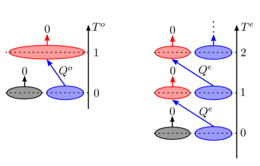
Figure 1: The action of the nilpotent operators $Q^{o}$ and $Q^{e}$ associated to a fermionic and bosonic ghost, respectively. The preimage of is drawn blue, the image in red.

Eq. (136) can be used very efficiently to compute the partition function (127) by means of the following trick. First, we compute the “free field” partition function over $\mathcal{C}$

$$\mathcal{Z}_{\mathcal{C}}\stackrel{{\scriptstyle\textup{\tiny def}}}{{=}}\text{str}_{\mathcal{C}}\left[u^{N_{t}}q^{E}\bar{q}^{\bar{E}}t^{T^{o}}\prod_{m=1}^{\infty}(t_{m}^{T^{o}_{m}}\bar{t}_{m}^{\bar{T}^{o}_{m}})\prod_{a}x_{a}^{D_{a}}\right]=\frac{1-t}{\text{sdet}(1-\mathbf{x}u)}\prod_{m=1}^{\infty}\frac{(1-t_{m})(1-\bar{t}_{m})}{|\text{sdet}(1-\mathbf{x}uq^{m})|^{2}}\ .$$ (137)

Next, we consider the decomposition of this partition function w.r.t. the action of $Q^{o}$

$$\mathcal{Z}_{\mathcal{C}}=\mathcal{Z}_{\mathsf{H}}+\mathcal{Z}_{\mathsf{Im}}+\mathcal{Z}_{\mathsf{Im}^{-1}}=\mathcal{Z}_{\mathsf{H}}+\mathcal{Z}_{\mathsf{Im}}(1-t^{-1}u^{2})\ ,$$ (138)

where $\mathcal{Z}_{\mathsf{H}}$, $\mathcal{Z}_{\mathsf{Im}}$ and $\mathcal{Z}_{\mathsf{Im}^{-1}}$ respectively denote the contribution of states in the cohomology, image and preimage of $Q^{o}$. We could express $Z_{\mathsf{Im}^{-1}}$ in terms of $Z_{\mathsf{Im}}$ since

$$\left[T\,,\,Q^{o}\right]=Q^{o}\ , \left[N\,,\,Q^{o}\right]=-2Q^{o}\ , \left[E\,,\,Q^{o}\right]=0\ , \left[\bar{E}\,,\,Q^{o}\right]=0\ ,$$

which follows from eqs. (130, 133). The weight $t$ keeps track of the ghost variable $c$ and is clearly unphysical. We can set $t=u^{2}$ and obtain from eq. (138)

$$\mathcal{Z}_{\mathcal{C}}\big{|}_{t=u^{2}}=Z_{\operatorname{\textsf{H}}}\big{|}_{t=u^{2}}=\mathcal{Z}_{\operatorname{\textsf{H}}^{Q^{o}}_{0}}\ .$$ (139)

The last equality is valid since the cohomology of $Q^{o}$ is localized exclusively at $T^{o}$-ghost number 0, hence it is independent of $t$. A similar argument applied to $Q^{o}_{m}$, $\bar{Q}^{o}_{m}$ gives

$$\mathcal{Z}_{\mathcal{C}}\big{|}_{t_{m}=u^{2}q^{m}}=\mathcal{Z}_{\operatorname{\textsf{H}}^{Q^{o}_{m}}_{0}}\ ,\qquad\mathcal{Z}_{\mathcal{C}}\big{|}_{\bar{t}_{m}=u^{2}\bar{q}^{m}}=\mathcal{Z}_{\operatorname{\textsf{H}}^{\bar{Q}^{o}_{m}}_{0}}\ .$$ (140)

The partition function in the combined cohomology is obtained by specializing the partition function (137) to the ghost weights appearing in eqs. (139, 140). This leads to the final result

$$\mathcal{Z}^{\text{free}}_{S^{M-1|2N}}(q,\bar{q}|u,\textbf{x})=\frac{1-u^{2}}{\text{sdet}(1-\mathbf{x}u)}\prod_{n=1}^{\infty}\frac{|1-u^{2}q^{n}|^{2}}{|\text{sdet}(1-\mathbf{x}uq^{n})|^{2}}\ .$$ (141)

A.2 $\mathcal{N}=1$ case

We shall apply the new method for the computation of free spectra that we have explained in detail in the previous section to the case of $\mathcal{N}=1$ world-sheet supersymmetric $S^{M-1|2N}$ superspheres. According to [48], we can replace in the action (90) all fields by superfields

$$\begin{split}X(z,\bar{z})&\mapsto X(Z,\bar{Z})=X(z,\bar{z})+\theta Y(z,\bar{z})+\bar{\theta}\bar{Y}(z,\bar{z})+\theta\bar{\theta}F(z,\bar{z})\ ,\\ \lambda(z,\bar{z})&\mapsto\lambda(Z,\bar{Z})=G(z,\bar{z})+\theta\sigma(z,\bar{z})+\bar{\theta}\bar{\sigma}(z,\bar{z})+\theta\bar{\theta}\lambda(z,\bar{z})\end{split}$$ (142)

and then integrate over the fermionic superspace variables to get the supersymmetric action

$$\mathcal{S}=\int\frac{d^{2}z}{\pi}\left[\partial X\cdot\bar{\partial}X+Y\cdot\bar{\partial}Y+\bar{Y}\cdot\partial\bar{Y}+F\cdot F+\lambda(X\cdot X-R^{2})+{}\right.\\ \left.{}+2\bar{\sigma}Y\cdot X-2\sigma\bar{Y}\cdot X+2G(F\cdot X-Y\cdot\bar{Y})\right]\ .$$ (143)

Next, we use the e.o.m. for the entire system (142) to eliminate the auxiliary field $F$ and the Lagrange multipliers $G$, $\sigma$, $\bar{\sigma}$ and $\lambda$. The output consists of the constraints

$$\chi\stackrel{{\scriptstyle\textup{\tiny def}}}{{=}}X\cdot X-R^{2}=0\ ,\quad\psi\stackrel{{\scriptstyle\textup{\tiny def}}}{{=}}X\cdot Y=0\ ,\quad\bar{\psi}\stackrel{{\scriptstyle\textup{\tiny def}}}{{=}}X\cdot\bar{Y}=0\ ,$$ (144)

together with the e.o.m. for $X$, $Y$ and $\bar{Y}$

$$\begin{split}\partial\bar{\partial}X&=-[(\partial X\cdot\bar{\partial}X)X+(\partial X\cdot\bar{Y})\bar{Y}+(\bar{\partial}X\cdot Y)Y]/R^{2}\ ,\\ \bar{\partial}Y&=-[(Y\cdot\bar{\partial}X)X+(Y\cdot\bar{Y})\bar{Y}]/R^{2}\ ,\quad\partial\bar{Y}=-[(\bar{Y}\cdot\partial X)X+(\bar{Y}\cdot Y)Y]/R^{2}\ .\end{split}$$ (145)

We shall now repeat the same steps as in the $\mathcal{N}=0$ case. First, we trade the world-sheet dependence of the fields $X$, $Y$, $\bar{Y}$ for the values of their higher order derivatives (118) and

$$Y_{m}\stackrel{{\scriptstyle\textup{\tiny def}}}{{=}}\partial^{m}Y(z,\bar{z})|_{z=z_{0}}\ ,\quad\bar{Y}_{m}\stackrel{{\scriptstyle\textup{\tiny def}}}{{=}}\bar{\partial}^{m}\bar{Y}(z,\bar{z})|_{z=z_{0}}\ ,\qquad(m\geq 0)$$ (146)

at some fixed point $z=z_{0}$. On-shell, all other derivatives can be expressed in terms of these ones using the e.o.m. (145). Next, we introduce a polynomial ring $s\mathcal{F}$ freely generated by the components of $X$, $X_{m}$, $\bar{X}_{m}$, $Y_{m}$ and $\bar{Y}_{m}$ and an ideal $s\mathcal{I}\subset s\mathcal{F}$ freely generated by the constraints (119) and

$$\psi_{m}\stackrel{{\scriptstyle\textup{\tiny def}}}{{=}}\partial^{m}\psi(z,\bar{z})|_{z=z_{0}}\ ,\quad\bar{\psi}_{m}\stackrel{{\scriptstyle\textup{\tiny def}}}{{=}}\bar{\partial}^{m}\bar{\psi}(z,\bar{z})|_{z=z_{0}}\ ,\qquad(m\geq 0)\ .$$ (147)

One can now identify the space of states of the $\mathcal{N}=1$ supersphere $\sigma$-model with the quotient $s\mathcal{H}\stackrel{{\scriptstyle\textup{\tiny def}}}{{=}}s\mathcal{F}/s\mathcal{I}$, because on-shell the most general derivatives of the constraints (144) are linear combinations of the free generators (119, 147) of $s\mathcal{I}$ with coefficients in $s\mathcal{F}$. The last part of the claim is proved as in the $\mathcal{N}=0$ case using the basic equations

$$\begin{split}\partial\bar{\partial}\chi(z,\bar{z})&=-\frac{2}{R^{2}}\left[(\partial X\cdot\bar{\partial}X)\chi+(\partial X\cdot\bar{Y})\bar{\psi}+(\bar{\partial}X\cdot Y)\psi\right](z,\bar{z})\ ,\\ \bar{\partial}\psi(z,\bar{z})&=-\frac{1}{R^{2}}\left[(Y\cdot\bar{\partial}X)\chi+(Y\cdot\bar{Y})\bar{\psi}\right](z,\bar{z})\ ,\\ \partial\bar{\psi}(z,\bar{z})&=-\frac{1}{R^{2}}\left[(\bar{Y}\cdot\partial X)\chi+(\bar{Y}\cdot Y)\psi\right](z,\bar{z})\ .\end{split}$$ (148)

Then we pass to the dual space $s\mathcal{H}^{*}$, which one can characterize as

$$s\mathcal{H}^{*}\simeq\operatorname{\textsf{Ker}}q^{o}\cap\bigcap_{m=1}^{\infty}(\operatorname{\textsf{Ker}}q^{o}_{m}\cap\operatorname{\textsf{Ker}}\bar{q}^{o}_{m})\cap\bigcap_{m=0}^{\infty}(\operatorname{\textsf{Ker}}q^{e}_{m}\cap\operatorname{\textsf{Ker}}\bar{q}^{e}_{m})\ ,$$ (149)

where $q^{e}_{m}$ and $q^{e}_{m}$ are the maps dual to the multiplication by $\psi_{m}$ and $\bar{\psi}_{m}$, respectively. Notice that the maps $q^{e}_{m}$ and $q^{e}_{m}$ are exact, because their duals are exact, i.e. the only elements of $s\mathcal{F}$ in the kernel of the multiplication by the odd constraints $\psi_{m}$ ($\bar{\psi}_{m}$) are those which are proportional to $\psi_{m}$ ($\bar{\psi}_{m}$). This observation, together with eq. (149) can be used to give a cohomological reformulation for $s\mathcal{H}$ just as in the $\mathcal{N}=0$ case.

Thus, besides the fermionic ghosts $c$, $c_{m}$, $\bar{c}_{m}$ introduced in the previous section, we associate to all fermionic constraints $\psi_{m}$ and $\bar{\psi}_{m}$ the corresponding bosonic ghosts $\gamma_{m}$ and $\bar{\gamma}_{m}$, and pass to the extended space $s\mathcal{C}\stackrel{{\scriptstyle\textup{\tiny def}}}{{=}}s\mathcal{F}^{*}\otimes s\mathcal{F}_{\text{gh}}$, where $s\mathcal{F}_{\text{gh}}$ is the polynomial ring generated by all ghosts. We then turn $s\mathcal{C}$ into a complex w.r.t. the nilpotent map

$$Q_{t}\stackrel{{\scriptstyle\textup{\tiny def}}}{{=}}Q^{o}_{t}+\sum_{m=0}^{\infty}(Q^{e}_{m}+\bar{Q}^{e}_{m})\ ,\qquad Q^{e}_{m}\stackrel{{\scriptstyle\textup{\tiny def}}}{{=}}q^{e}_{m}\otimes\gamma_{m}\ ,\qquad\bar{Q}^{e}_{m}\stackrel{{\scriptstyle\textup{\tiny def}}}{{=}}\bar{q}^{e}_{m}\otimes\bar{\gamma}_{m}\ .$$ (150)

Once again, the cohomology of $Q_{t}$ lies in the combined cohomology of its elementary summands, because the latter anticommute with each other. Moreover, the exactness of $q^{e}_{m}$ ($\bar{q}^{e}_{m}$) implies that the cohomology of $Q^{e}_{m}$ ($\bar{Q}^{e}_{m}$) also lies at $\gamma_{m}$-ghost number 0, see fig. 1. Thus, on the one hand, we conclude that the cohomology of $Q_{t}$ lies exclusively at total ghost number 0, while on the other hand eq. (149) (see also fig. 1) implies that it coincides with $s\mathcal{H}^{*}$.

One can now use the same trick as in the previous section to derive the partition function of $s\mathcal{H}\simeq s\mathcal{H}^{*}$ from the “free field” partition function of $s\mathcal{C}$

$$s\mathcal{Z}_{s\mathcal{C}}=\frac{1-t}{\text{sdet}(1-\mathbf{x}u)}\prod_{m=1}^{\infty}\frac{(1-t_{m})(1-\bar{t}_{m})}{|\text{sdet}(1-\mathbf{x}uq^{m})|^{2}}\times\prod_{m=0}^{\infty}\frac{|\text{sdet}(1-\mathbf{x}uq^{m+\frac{1}{2}})|^{2}}{(1-\tau_{m})(1-\bar{\tau}_{m})}\ ,$$ (151)

where every bosonic ghost $\gamma_{m}$ ($\bar{\gamma}_{m}$) is weighted by a factor of $\tau_{m}$ ($\bar{\tau}_{m}$). Arguing as before, one concludes that by setting the ghost weights to the special values (139, 140) and

$$\tau_{m}=u^{2}q^{m+\frac{1}{2}}\ ,\quad\bar{\tau}_{m}=u^{2}\bar{q}^{m+\frac{1}{2}}\ ,$$ (152)

only the elements in the cohomology of $Q_{t}$ contribute. Inserting these values in eq. (151) we obtain the final result

$$s\mathcal{Z}^{\text{free}}_{S^{M-1|2N}}(q,\bar{q}\,|\,\mathbf{x})=\frac{1-u^{2}}{\text{sdet}(1-\mathbf{x}u)}\prod_{n=1}^{\infty}\left|\frac{1-u^{2}q^{n}}{1-u^{2}q^{n-\frac{1}{2}}}\frac{\text{sdet}(1-\mathbf{x}uq^{n-\frac{1}{2}})}{\text{sdet}(1-\mathbf{x}uq^{n})}\right|^{2}\ .$$ (153)

Appendix B An integral identity

For the reader’s convenience, we have assembled in this appendix the derivation of the integral formula (52). For this, we use Stokes’ theorem and arrive at

$$\int_{\mathbb{C}_{\epsilon}}\frac{d^{2}z}{\pi}\frac{1}{(z-x)(z-y)(\bar{z}-\bar{x})(\bar{z}-\bar{y})} = \frac{1}{\bar{x}-\bar{y}}\int_{\mathbb{C}_{\epsilon}}\frac{d^{2}z}{\pi}\bar{\partial}_{z}\frac{\log\left|\frac{z-x}{z-y}\right|^{2}}{(z-x)(z-y)}$$ (154)

$$= -\frac{1}{\bar{x}-\bar{y}}\oint_{\partial\mathbb{C}_{\epsilon}}\frac{dz}{2\pi i}\frac{\log\left|\frac{z-x}{z-y}\right|^{2}}{(z-x)(z-y)}\ ,$$

where in the last line the contour integral has two counterclockwise oriented pieces – the first around $x$ and the second around $y$ – both of which give the same contribution. Performing this integrals is easy and leads to

$$\int_{\mathbb{C}_{\epsilon}}\frac{d^{2}z}{\pi}\frac{1}{(z-x)(z-y)(\bar{z}-\bar{x})(\bar{z}-\bar{y})}=\frac{2\log\left|\frac{x-y}{\epsilon}\right|^{2}}{|x-y|^{2}}+\mathcal{O}(\epsilon)\ .$$ (155)

By taking now the appropriate number of derivatives in $x$, $y$, $\bar{x}$ or $\bar{y}$ on both sides of the above equation, we recover eq. (52).

Appendix C A combinatorial identity

In this appendix we shall prove the combinatorial identity (114), namely

$$\frac{\prod_{j}\det(1-\mathbf{y}w_{j})}{\prod_{j}\det(1-\mathbf{y}v_{j})}\prod_{i\leq j}(1-v_{i}v_{j})\prod_{i<j}(1-w_{i}w_{j})=\prod_{i,j}(1-v_{i}w_{j})\sum_{\mu}sb_{\mu}(\mathbf{y})s_{\mu}(\mathbf{v}|\mathbf{w})\ ,$$

where $\mathbf{y}$ is an SO$(2n+1)$ matrix, $\mathbf{v}=(v_{1},v_{2},\dots)$ and $\mathbf{w}=(w_{1},w_{2},\dots)$ are possibly infinite vectors and $s_{\mu}(\mathbf{v}|\mathbf{w})$ are the supersymmetric Schur functions defined by the expansion

$$\prod_{i,j}\frac{(1-v_{i}w^{\prime}_{j})(1-v^{\prime}_{i}w_{j})}{(1-v_{i}v^{\prime}_{j})(1-w_{i}w^{\prime}_{j})}=\sum_{\mu}s_{\mu}(\mathbf{v}|\mathbf{w})s_{\mu}(\mathbf{v}^{\prime}|\mathbf{w}^{\prime})\ .$$ (156)

They satisfy the defining property $s_{\lambda}s_{\mu}=\sum_{\nu}c_{\lambda\mu}^{\nu}s_{\nu}$ of the Schur functions and can be expressed in terms of the “bosonic” Schur functions as

$$s_{\lambda}(\mathbf{v}|\mathbf{w})=\sum_{\mu,\nu}c^{\lambda}_{\mu\nu}s_{\mu}(\mathbf{v})s_{\nu^{t}}(-\mathbf{w})\ ,$$ (157)

see eqs. (A.7) and (A.10) of [49]. We shall also need the identities [50]

$$\prod_{i\leq j}(1-v_{i}v_{j})=\sum_{\rho\in R}(-1)^{\frac{|\rho|}{2}}s_{\rho}(\mathbf{v})\ ,\qquad\prod_{i<j}(1-w_{i}w_{j})=\sum_{\rho\in R}(-1)^{\frac{|\rho|}{2}}s_{\rho^{t}}(\mathbf{w})\ ,$$ (158)

where $|\rho|$ is the number of boxes in $\rho$ and $R$ is the set of partitions for which every $i$-th row is one box longer then the respective $i$-th column. In particular, all $\rho\in R$ have an even number of boxes. Notice that together eqs. (78, 158) imply the well known relation between the SO$(2n+1)$ and $\mathrm{SU}(2n+1)$ characters, see e.g. [42],

$$sb_{\lambda}(\mathbf{y})=\sum_{\mu}\sum_{\rho\in R}(-1)^{\frac{|\rho|}{2}}c^{\lambda}_{\rho\mu}s_{\mu}(\mathbf{y})\ .$$ (159)

Furthermore, using eq. (158), the “dual” Cauchy identity

$$\prod_{j}\det(1+\mathbf{y}w_{j})=\sum_{\lambda}s_{\lambda}(\mathbf{y})s_{\lambda^{t}}(\mathbf{w})\ ,$$ (160)

and then the relation (159) one can prove the “dual” of eq. (78)

$$\prod_{j}\det(1+\mathbf{y}w_{j})\prod_{i<j}(1-w_{i}w_{j})=\sum_{\lambda}sb_{\lambda}(\mathbf{y})s_{\lambda^{t}}(\mathbf{w})\ .$$ (161)

The identity (114) can now be proved as follows

$$\frac{\prod_{j}\det(1-\mathbf{y}w_{j})}{\prod_{j}\det(1-\mathbf{y}v_{j})}\prod_{i\leq j}(1-v_{i}v_{j})\prod_{i<j}(1-w_{i}w_{j})=\sum_{\lambda,\mu}sb_{\lambda}(\mathbf{y})sb_{\mu}(\mathbf{y})s_{\lambda}(\mathbf{v})s_{\mu^{t}}(-\mathbf{w})=$$

$$=\mathop{\sum_{\lambda,\mu,\nu}}_{\alpha,\beta,\gamma}c^{\lambda}_{\alpha\beta}c^{\mu}_{\beta\gamma}c^{\nu}_{\gamma\alpha}sb_{\nu}(\mathbf{y})s_{\lambda}(\mathbf{v})s_{\mu^{t}}(-\mathbf{w})=\mathop{\sum_{\nu,\alpha}}_{\beta,\gamma}c^{\nu}_{\gamma\alpha}sb_{\nu}(\mathbf{y})s_{\alpha}(\mathbf{v})s_{\beta}(\mathbf{v})s_{\beta^{t}}(-\mathbf{w})s_{\gamma^{t}}(-\mathbf{w})=$$

$$=\prod_{i,j}(1-v_{i}w_{j})\sum_{\alpha,\gamma,\nu}c^{\nu}_{\gamma\alpha}sb_{\nu}(\mathbf{y})s_{\alpha}(\mathbf{v})s_{\gamma^{t}}(-\mathbf{w})=\prod_{i,j}(1-v_{i}w_{j})\sum_{\nu}sb_{\nu}(\mathbf{y})s_{\nu}(\mathbf{v}|\mathbf{w})\ ,$$

were the first equality follows from eqs. (78, 160), in the second equality we have used the Newell-Littlewood formula (83), in the fourth equality the dual Cauchy identity (161) and in the last equality the restriction formula (157) for the supersymmetric Schur functions.

References

- [1] A. M. Polyakov, Interaction of Goldstone Particles in Two-Dimensions. Applications to Ferromagnets and Massive Yang-Mills Fields, Phys. Lett. B, 59:79, 1975.
- [2] E. Brézin and J. Zinn-Justin, Renormalization of the nonlinear -model in dimensions. Application to the Heisenberg ferromagnets, Phys. Rev. Lett., 36:691, 1976.
- [3] D. H. Friedan, Nonlinear Models in Dimensions, Annals Phys., 163:318, 1985.
- [4] A. D’Adda, M. Lüscher and P. Di Vecchia, A Expandable Series of Nonlinear -models with Instantons, Nucl. Phys. B, 146:63, 1978.
- [5] C. G. Callan, Jr. and L. Thorlacius, Sigma Models And String Theory , In Providence 1988, Proceedings, Particles, strings and supernovae, vol. 2*:795-878, 1988.
- [6] E. H. Fradkin, Field theories of condensed matter systems, Redwood City, USA: Addison-Wesley(Frontiers in physics, 82), 350p, 1991.
- [7] A. M. Tsvelik, Quantum field theory in condensed matter physics, Cambridge, UK: Univ. Pr., 332 p, 1995.
- [8] A. A. Tseytlin, On -model RG flow, ’central charge’ action and Perelman’s entropy, Phys. Rev. D, 75:064024, 2007, hep-th/0612296.
- [9] J. M. Evans, D. Kagan, N. J. MacKay and C. A. S. Young, Quantum, higher-spin, local charges in symmetric space -models, JHEP, 0501:020, 2005, hep-th/0408244.
- [10] A. Babichenko, Conformal invariance and quantum integrability of -models on symmetric superspaces, Phys. Lett. B, 648:254, 2007, hep-th/0611214.
- [11] I. Bena, J. Polchinski and R. Roiban, Hidden symmetries of the superstring, Phys. Rev. D, 69:046002, 2004, hep-th/0305116.
- [12] C. A. S. Young, Non-local charges, gradings and coset space actions, Phys. Lett. B, 632:559, 2006, hep-th/0503008.
- [13] I. Jack, D. R. T. Jones and N. Mohammedi, A Four Loop Calculation Of The Metric Beta Function For The Bosonic -model And The String Effective Action, Nucl. Phys. B, 322:431, 1989.
- [14] C. Candu. Discrétisation des modèles sigma invariants conformes sur des supersphères et superespaces projectifs. PhD thesis, Université Paris 6, 2008.
- [15] C. Candu, T. Creutzig, V. Mitev, and V. Schomerus, Cohomological Reduction of -models, JHEP, 05:047, 2010, arXiv:1001.1344.
- [16] M. Bershadsky, S. Zhukov, and A. Vaintrob, PSL(nn) -model as a conformal field theory, Nucl. Phys., B559:205–234, 1999, hep-th/9902180.
- [17] N. Berkovits, C. Vafa, and E. Witten, Conformal field theory of AdS background with Ramond-Ramond flux, JHEP, 03:018, 1999.
- [18] V. Serganova, Classification of real simple Lie superalgebras and symmetric superspaces, Funct. Anal. Appl., 17:200, 1983.
- [19] C. Candu and V. Schomerus, Exactly marginal parafermions, Phys.Rev. D, 84:051704, 2011, arXiv:1104.5028.
- [20] C. Candu, V. Tlapác and V. Schomerus, CFT and Hermitian symmetric superspaces, in preparation.
- [21] D. Nemeschansky and A. Sen, Conformal invariance of supersymmetric -models on Calabi-Yau manifolds, Phys. Lett. B, 178:365, 1986.
- [22] F. Wegner, Anomalous Dimensions For The Nonlinear -model in -dimensions. 1, Nucl. Phys. B, 280:193, 1987.
- [23] F. Wegner, Anomalous Dimensions For The Nonlinear -model in -dimensions. 2, Nucl. Phys. B, 280:210, 1987.
- [24] E. Brézin, J. Zinn-Justin and J. C. Le Guillou, Anomalous Dimensions of Composite Operators Near Two-Dimensions for Ferromagnets with Symmetry, Phys. Rev. B, 14:4976, 1976.
- [25] F. Wegner, Anomalous dimensions of high-gradient operators in the n-vector model in dimensions, Zeitschrift für Phys. B, Cond. Mat., 78:1, 1990.
- [26] H. Mall and F. Wegner, Anomalous dimensions of high gradient operators in the orthogonal matrix model, Nucl. Phys. B, 393:495, 1993.
- [27] F. Wegner, Anomalous dimensions of high gradient operators in the unitary matrix model, Nucl. Phys. B, 354:441, 1991.
- [28] T. Quella, V. Schomerus, and T. Creutzig, Boundary Spectra in Superspace Sigma-Models, JHEP, 10:024, 2008, arXiv:0712.3549.
- [29] C. Candu and H. Saleur, A lattice approach to the conformal OSp supercoset sigma model. Part I: Algebraic structures in the spin chain. The Brauer algebra, Nucl. Phys. B, 808:441–486, 2009, arXiv:0801.0430.
- [30] C. Candu and H. Saleur, A lattice approach to the conformal supercoset -model. Part II: The boundary spectrum, Nucl. Phys. B, 808:487–524, 2009, arXiv:0801.0444.
- [31] V. Mitev, T. Quella, and V. Schomerus, Principal Chiral Model on Superspheres, JHEP, 11:086, 2008, arXiv:0809.1046.
- [32] C. Candu, V. Mitev, T. Quella, H. Saleur, and V. Schomerus, The -model on Complex Projective Superspaces, JHEP, 02:015, 2010, arXiv:0908.0878.
- [33] J. Honerkamp, F. Krause and M. Scheunert, On the equivalence of standard and covariant perturbation series in non-polynomial pion lagrangian field theory, Nucl. Phys. B, 69:618, 1974.
- [34] L. Álvarez-Gaumé, D. Z. Freedman and S. Mukhi, The Background Field Method and the Ultraviolet Structure of the Supersymmetric Nonlinear -model, Annals Phys., 134:85, 1981.
- [35] K. Pilch and A. N. Schellekens, Formulae For The Eigenvalues Of The Laplacian On Tensor Harmonics On Symmetric Coset Spaces, J. Math. Phys., 25:3455, 1984.
- [36] C. Candu, V. Mitev, and V. Schomerus. Anomalous Dimensions in Deformed WZW Models on Supergroups. JHEP, 1303:003, 2013.
- [37] D. Kagan, and C. Young, Conformal Sigma-Models on Supercoset Targets. Nucl. Phys. B, 745:109-122, 2006.
- [38] R. Bott Homogeneous vector bundles. Ann. of Math., Second Series, Vol.66, No. 2 203, 1957.
- [39] M. R. Zirnbauer, Riemannian symmetric superspaces and their origin in random-matrix theory, J. Math. Phys., 37:4986, 1996.
- [40] V. Schomerus and H. Saleur. The GL(11) WZW model: From supergeometry to logarithmic CFT. Nucl. Phys. B, 734:221–245, 2006, arXiv:hep-th/0510032.
- [41] G. Benkart, C. L. Shader, and A. Ram. Tensor product representations for orthosymplectic Lie superalgebras. J. Pure Appl. Algebra, 130:1-48, 1998.
- [42] K. Koike and I. Terada, Young-Diagrammatic methods for the representation theory of the classical groups of type , , , J. Algebra, 107:466, 1987.
- [43] H. Boerner, Representations of groups. North-Holland Publishing Company, 1963.
- [44] R. C. King, Modification rules and products of irreducible representations of the unitary, orthogonal, and symplectic groups, J. Math. Phys., 12:1588, 1971.
- [45] A. B. Balantekin and I. Bars, Dimension and Character Formulas for Lie Supergroups, J. Math. Phys., 22:1149, 1981.
- [46] G. Barnich, F. Brandt, and M. Henneaux, Local BRST cohomology in gauge theories. Phys.Rept., 338:439-569, 2000. hep-th/0002245.
- [47] P. Gao, and M. R. Douglas, Geodesics on Calabi-Yau manifolds and winding states in nonlinear -models, arXiv:1301.1687.
- [48] E. Witten, A Supersymmetric Form of the Nonlinear -model in Two-Dimensions, Phys. Rev. D, 16:2991, 1977.
- [49] C. Candu and M. R. Gaberdiel, Supersymmetric holography on , arXiv:1203.1939.
- [50] I. G. MacDonald, Symmetric functions and Hall polynomials, Oxford University Press, 1979.