Effective field theory for proton halo nuclei

Abstract

We use halo effective field theory to analyze the universal features of proton halo nuclei bound due to a large S-wave scattering length. With a Lagrangian built from effective core and valence-proton fields, we derive a leading-order expression for the charge form factor. Within the same framework we also calculate the radiative proton capture cross section. Our general results at leading order are applied to study the excited $1/2^{+}$ state of Fluorine-17, and we give results for the charge radius and the astrophysical S-factor.

1 Introduction

Exotic isotopes along the neutron and proton drip lines are important for our understanding of the formation of elements and they constitute tests of our understanding of nuclear structure. The proton- and neutron-rich regimes in the chart of nuclei are therefore the focus of existing and forthcoming experimental facilities around the world [1]. The emergence of new degrees of freedom is one important feature of these systems; exemplified, e.g., by the discovery of several nuclear halo states along the drip lines [2, 3, 4]. Halo states in nuclei are characterized by a tightly bound core with weakly attached valence nucleon(s). Universal structures of such states can be considered a consequence of quantum tunneling, where tightly-bound clusters of nucleons behave coherently at low energies and the dynamics is dominated by relative motion at distances beyond the region of the short-range interaction. In the absence of the Coulomb interaction, it is known that halo nuclei bound due to a large positive S-wave scattering length will show universal features [5, 6]. In the case of proton halo nuclei, however, the Coulomb interaction introduces an additional momentum scale $k_{\mathrm{C}}$, which is proportional to the charge of the core and the reduced mass of the halo system. The low-energy properties of proton halos strongly depend on $k_{\mathrm{C}}$.

Halo effective field theory (EFT) is the ideal tool to analyze the features of halo states with a minimal set of assumptions. It describes these systems using their effective degrees of freedom, i.e. core and valence nucleons, and interactions that are dictated by low-energy constants [7, 8]. For S-wave proton halo systems there will be a single unknown coupling constant at leading order, and this parameter can be determined from the experimental scattering length, or the one-proton separation energy. Obviously, halo EFT is not intended to compete with ab initio calculations that, if applicable, would aim to predict low-energy observables from computations starting with a microscopic description of the many-body system. Instead, halo EFT is complementary to such approaches as it provides a low-energy description of these systems in terms of effective degrees of freedom. This reduces the complexity of the problem significantly. By construction, it can also aid to elucidate the relationship between different low-energy observables.

Furthermore, halo EFT is built on fields for clusters, which makes it related to phenomenological few-body cluster models [3]. The latter have often been used successfully for confrontation with data for specific processes involving halo nuclei. A relevant example in the current context is the study of proton radiative capture into low-lying states states of ¹⁷F [9]. A general discussion of electromagnetic reactions of proton halos in a cluster approach was given in [10]. The emphasis of an EFT, however, is the systematic expansion of the most general interactions and, as a consequence, the ability to estimate errors and to improve predictions order by order. The structure and reactions of one- and two-neutron halos have been studied in halo EFT over the last years (see, e.g., Refs. [11, 12, 13, 14, 15, 16, 17]). However, concerning charged systems only unbound states such as $\alpha\alpha$ [18] and $\alpha p$ [19] have been treated in halo EFT.

In this letter, we apply halo EFT for the first time to one-proton halo nuclei. We restrict ourselves to leading order calculations of systems that are bound due to a large S-wave scattering length between the core and the proton. The manuscript is organized as follows: In Sec. 2, we introduce the halo EFT and discuss how Coulomb interactions are treated within this framework. In the following section, we present our results and calculate, in particular, the charge form factor and charge radius at leading order. Furthermore, we derive expressions for the radiative capture cross section. We apply our general formulae to the excited $1/2^{+}$ state of ¹⁷F and compare our numerical results with existing data for this system. We conclude with an outlook and a discussion on the importance of higher-order corrections.

2 Theory

In halo EFT, the core and the valence nucleons are taken as the degrees of freedom. For a one-proton halo system, the Lagrangian is given by

$$\mathcal{L}=\sum_{k=0,1}\psi_{k}^{\dagger}\left(i\mathrm{D}_{0}+\frac{\mathbf{D}^{2}}{2m_{k}}\right)\psi_{k}-C_{0}\psi_{0}^{\dagger}\psi_{1}^{\dagger}\psi_{1}\psi_{0}+\ldots$$ (1)

Here $\psi_{0}$ denotes the proton field with mass $m_{0}$ and $\psi_{1}$ the core field with mass $m_{1}$, $C_{0}$ denotes the leading order (LO) coupling constant, and the dots denote derivative operators that facilitate the calculation of higher order corrections. The covariant derivative is defined as $\mathrm{D}_{\mu}:=\partial_{\mu}+ie\hat{\mathrm{Q}}A_{\mu}~{}$, where $\hat{\mathrm{Q}}$ is the charge operator. The resulting one-particle propagator is given by

$$iS_{k}(p_{0},\mathbf{p})=i\left[p_{0}-\frac{\mathbf{p}^{2}}{2m_{k}}+i\varepsilon\right]^{-1}~{}.$$ (2)

For convenience, we will also define the proton-core two-particle propagator

$$iS_{\rm tot}(p_{0},\mathbf{p})=i\left[p_{0}-\frac{\mathbf{p}^{2}}{2m_{\rm R}}+i\varepsilon\right]^{-1}~{},$$ (3)

where $m_{\rm R}$ denotes the reduced mass of the proton-core system. We include the Coulomb interaction through the full Coulomb Green’s function

$$\langle\mathbf{k}|G_{\mathrm{C}}(E)|\mathbf{p}\rangle=-S_{\rm tot}(E,\mathbf{k})\chi(\mathbf{k},\mathbf{p};E)S_{\rm tot}(E,\mathbf{p})~{},$$ (4)

Figure 1: The integral equation for the four-point function $\chi(\mathbf{k}_{1},\mathbf{k}_{2})~{}$. The dashed line denotes a core propagator, the solid line a proton propagator and the wave line denotes the exchange of a Coulomb photon.

where $\chi$ is the Coulomb four-point function defined recursively in Fig. 1. To distinguish coordinate space from momentum space states we will denote the former with round brackets, i.e. $(\mathbf{r}|$. In coordinate space, the Coulomb Green’s function can be expressed via its spectral representation

$$(\mathbf{r}|G_{\mathrm{C}}(E)|\mathbf{r}^{\prime})=\int\frac{\mathrm{d}^{3}p}{(2\pi)^{3}}\frac{\psi_{\mathbf{p}}(\mathbf{r})\psi^{*}_{\mathbf{p}}(\mathbf{r}^{\prime})}{E-\mathbf{p}^{2}/(2m_{\mathrm{R}})+i\varepsilon}~{},$$ (5)

where we define the Coulomb wave function through its partial wave expansion

$$\psi_{\mathbf{p}}(\mathbf{r})=\sum_{l=0}^{\infty}(2l+1)i^{l}\exp{(i\sigma_{l})\frac{F_{l}(\eta,\rho)}{\rho}P_{l}(\hat{\mathbf{p}}\cdot\hat{\mathbf{r}})}~{}.$$ (6)

Here we have defined $\rho=pr$ and $\eta=k_{\mathrm{C}}/p~{},$ with the Coulomb momentum $k_{\mathrm{C}}=Z_{\mathrm{c}}\alpha m_{\mathrm{R}}~{},$ and also the pure Coulomb phase shift $\sigma_{l}=\arg{\Gamma(l+1+i\eta)}~{}.$ For the Coulomb functions $F_{l}$ and $G_{l}$, we use the conventions of Ref. [20]. The regular Coulomb function $F_{l}$ can be expressed in terms of the Whittaker M-function according to

$$F_{l}(\eta,\rho)=A_{l}(\eta)M_{i\eta,l+1/2}(2i\rho)~{},$$ (7)

with the $A_{l}$ defined as

$$A_{l}(\eta)=\frac{|\Gamma{(l+1+i\eta)}|\exp{\left[-\pi\eta/2-i(l+1)\pi/2\right]}}{2(2l+1)!}~{}.$$ (8)

We shall also need the irregular Coulomb wave function, $G_{l}$, which is given by

$$G_{l}(\eta,\rho)=iF_{l}(\eta,\rho)+B_{l}(\eta)W_{i\eta,l+1/2}(2i\rho)~{},$$ (9)

where $W$ is the Whittaker W-function and the coefficient $B_{l}$ is defined as

$$B_{l}(\eta)=\frac{\exp{(\pi\eta/2+il\pi/2)}}{\arg{\Gamma{(l+1+i\eta)}}}~{}.$$ (10)

To obtain the fully-dressed two-particle propagator, that includes strong and Coulomb interactions, we calculate the irreducible self-energy shown in Fig. 2.

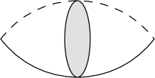
Figure 2: The irreducible self-energy at leading order. The solid (dashed) line denotes the proton (core) propagator. The shaded blob denotes the Coulomb Green’s function.

$$i\Sigma(E) = -i\int\frac{\mathrm{d}^{3}k_{1}\mathrm{d}^{3}k_{2}}{(2\pi)^{6}}S_{\rm tot}(E,\mathbf{k}_{1})\chi(\mathbf{k}_{1},\mathbf{k}_{2})S_{\rm tot}(E,\mathbf{k}_{2})$$ (11)

$$= i(0|G_{\mathrm{C}}(E)|0)~{}.$$

The expression above is known and is given by

$$(0|G_{\mathrm{C}}(E)|0)=-2m_{R}\int\frac{\mathrm{d}^{3}q}{(2\pi)^{3}}\frac{\psi_{\mathbf{q}}(0)\psi^{*}_{\mathbf{q}}(0)}{q^{2}-2m_{R}E-i\varepsilon}~{}.$$ (12)

This integral was solved in Ref. [21], using dimensional regularization in the power divergence subtraction (PDS) scheme, as

$$\Sigma(E)=-\frac{k_{\mathrm{C}}m_{\mathrm{R}}}{\pi}H(\eta)+\Sigma^{\mathrm{div}}~{},$$ (13)

with a divergent part $\Sigma^{\mathrm{div}}$

$$\Sigma^{\mathrm{div}}=\frac{k_{\mathrm{C}}m_{\mathrm{R}}}{\pi}\left[\frac{1}{3-d}+\log\left({\frac{\sqrt{\pi}\mu}{2k_{\mathrm{C}}}}\right)+1-\frac{3C_{\mathrm{E}}}{2}\right]-\frac{m_{\mathrm{R}}\mu}{2\pi}~{},$$ (14)

where $d$ is the space dimension, $C_{\mathrm{E}}$ is the Euler constant, and $\mu$ is the PDS regulator. The function $H$ is defined as

$$H(\eta)=\psi(i\eta)+\frac{1}{2i\eta}-\log{(i\eta)}~{},$$ (15)

with $\psi$ being the polygamma function. Note that the divergent part in Eq. (14) is energy independent. This will become important later when the derivative of $\Sigma$, with respect to the energy, will be required.

The coupling constant $C_{0}$ can be determined by matching to a two-body observable, such as the Coulomb corrected proton-core scattering length [21]:

$$\frac{1}{a_{\mathrm{C}}}=\frac{2\pi}{m_{\mathrm{R}}}\left(\frac{1}{C_{0}}-\Sigma^{\mathrm{div}}\right)~{}.$$ (16)

Since we stay at leading order, however, an explicit expression for $C_{0}$ will not be required for the calculation of electromagnetic observables in the next section.

3 Results

3.1 Charge Form Factor

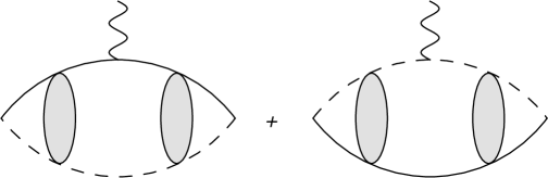
Figure 3: The irreducible three-point function $\Gamma^{0}~{}$.

In our calculation of the charge form factor, we follow the derivation of the deuteron form factor presented in Ref. [22]. The form factor is obtained by calculating the matrix element

$$\langle\mathbf{p}^{\prime}|J^{0}_{\mathrm{EM}}|\mathbf{p}\rangle=e(Z_{c}+1)F_{\mathrm{C}}(\mathbf{Q}^{2})~{},$$ (17)

for momentum transfer $\mathbf{Q}=\mathbf{p}^{\prime}-\mathbf{p}$ in the Breit frame, where no energy is transferred by the photon. It was shown in Ref. [22] that this matrix element can be expressed as

$$\langle\mathbf{p}^{\prime}|J^{0}_{\mathrm{EM}}|\mathbf{p}\rangle = \frac{\Gamma^{0}(\mathbf{Q})}{\Sigma^{\prime}(-B)}~{},$$ (18)

where $\Gamma^{0}$ denotes the irreducible three-point function shown in Fig. 3, and $\Sigma^{\prime}(-B)$ is the derivative of the self-energy with respect to the total energy evaluated at the energy $E=-B~{}$, where $B$ is the proton separation energy or core-proton binding energy.

With the proton-core mass ratio $f=m_{0}/m_{1}~{}$, the three-point function $\Gamma^{0}$ is given by

$$\Gamma^{0}(\mathbf{Q}) = -eZ_{\mathrm{c}}\int\mathrm{d}^{3}r\exp{(if\mathbf{Q}\cdot\mathbf{r})}|(0|G_{\mathrm{C}}(-B)|\mathbf{r})|^{2}$$ (19)

$$+\Big{[}(f\to 1-f),~{}(Z_{\mathrm{c}}\to 1)\Big{]}~{},$$

and the derivative of the self-energy can be written as

$$\Sigma^{\prime}(-B)=-\int\frac{\mathrm{d}^{3}q}{(2\pi)^{3}}\frac{\psi_{\mathbf{q}}(0)\psi^{*}_{\mathbf{q}}(0)}{(B+\mathbf{q}^{2}/(2m_{R}))^{2}}~{}.$$ (20)

Evaluating $\Gamma^{0}$ at zero momentum transfer, by using Eq. (5) and orthonormality of the wavefunctions, and comparing with Eq. (20) shows that the charge form factor is properly normalized to one in this limit.

We find that Eq. (19) can be simplified by writing the Coulomb Green’s function for negative energy using the Whittaker W-function. This is achieved by demanding proper asymptotics and using that only the S-wave part can contribute to propagation to zero separation, that is

$$(0|G_{\mathrm{C}}(-B)|\mathbf{r}) = \lim_{\rho^{\prime}\to 0}\left(-i\frac{m_{\mathrm{R}}\gamma_{0}}{2\pi}\frac{F_{0}(\eta,\rho^{\prime})\left[iF_{0}(\eta,\rho)+G_{0}(\eta,\rho)\right]}{\rho^{\prime}\rho}\right)$$ (21)

$$= i\frac{m_{\mathrm{R}}\Gamma(1+k_{\mathrm{C}}/\gamma_{0})}{2\pi}\frac{W_{-k_{\mathrm{C}}/\gamma_{0},1/2}(2\gamma_{0}r)}{r}~{},$$

where we have introduced the binding momentum $\gamma_{0}=\sqrt{2m_{\mathrm{R}}B}$. The resulting integral is then

$$\Gamma^{0}(\mathbf{Q}) = -\frac{em_{\mathrm{R}}^{2}\Gamma(1+k_{\mathrm{C}}/\gamma_{0})^{2}}{\pi}\int\hbox{d}r\left[Z_{\mathrm{c}}j_{0}\Big{(}fQr\Big{)}+j_{0}\Big{(}(1-f)Qr\Big{)}\right]$$ (22)

$$\times W_{-k_{\mathrm{C}}/\gamma_{0},1/2}(2\gamma_{0}r)^{2}~{},$$

where $j_{l}$ are the spherical Bessel functions. Once the parameters of the proton halo system are fixed, the equation

$$F_{\mathrm{C}}(\mathbf{Q}^{2})=\frac{\Gamma^{0}(\mathbf{Q})}{e(Z_{c}+1)\Sigma^{\prime}(-B)}$$ (23)

is used to calculate the charge form factor and the corresponding charge radius numerically. We have calculated these quantities for the excited $1/2^{+}$ state of ¹⁷F, which has a proton separation energy of $B=104.94~{}(35)~{}\mathrm{keV}~{}$[23]. Note that the proton separation energy is the only non-trivial experimental input at LO.

The charge form factor is related to the charge radius via the expansion

$$F_{\mathrm{C}}(\mathbf{Q}^{2})=1-\frac{\langle r_{\mathrm{C}}^{2}\rangle_{\mathrm{rel}}}{6}\mathbf{Q}^{2}+\ldots~{},$$ (24)

and we find for the charge radius squared

$$\langle r_{\mathrm{C}}^{2}\rangle_{\mathrm{rel}}=(0.59~{}\mathrm{fm})^{2}~{}.$$ (25)

Since the proton and core are treated as structureless fields in halo EFT, this quantity corresponds to the charge radius difference according to

$$\langle r_{\mathrm{C}}^{2}\rangle_{{}^{17}\mathrm{F}^{*}}=\frac{Z_{\mathrm{c}}}{Z_{\mathrm{c}}+1}\langle r_{\mathrm{C}}^{2}\rangle_{{}^{16}\mathrm{O}}+\frac{1}{Z_{\mathrm{c}}+1}\langle r_{\mathrm{C}}^{2}\rangle_{\mathrm{p}}+\langle r_{\mathrm{C}}^{2}\rangle_{\mathrm{rel}}~{},$$ (26)

where $\langle r_{\mathrm{C}}^{2}\rangle_{\mathrm{X}}$ is the charge radius squared corresponding to the particle $\mathrm{X}={}^{17}\mathrm{F}^{*}$, ¹⁶O, $\mathrm{p}$. Analog to the deuteron case, the charge radii of proton and ¹⁶O enter at higher orders in the calculation via counter terms.

The error of the EFT can be estimated by comparing the momentum scale $k_{\mathrm{lo}}\sim\gamma_{0}$ of the halo with the break-down scale $k_{\mathrm{hi}}$ of the EFT. The latter is given by the closest interfering state. For the ¹⁷F halo system the break-down scale is given by the bound state, $E_{0}=495.33~{}(10)~{}\mathrm{keV}~{}$ below the $1/2^{+}$ state [23]. Thus, the expected LO error is $\gamma_{0}/\sqrt{2m_{\mathrm{R}}E_{0}}\approx 1/2$ for the halo state in ¹⁷F^∗, which is comparable to the LO error of a pionless EFT calculation for the two-nucleon system.

3.2 Radiative Capture

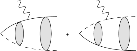
Figure 4: The radiative proton capture diagrams.

Our approach can easily be applied to low-energy radiative capture. The differential cross section for this reaction is

$$\frac{\mathrm{d}\sigma}{\mathrm{d}\Omega}=\frac{m_{\mathrm{R}}\omega}{8\pi^{2}p}\sum_{i=1}^{2}\left|\epsilon_{i}\cdot\frac{\mathcal{A}}{\sqrt{\Sigma^{\prime}(-B)}}\right|^{2}~{},$$ (27)

where $\mathcal{A}$ is the vector amplitude for the sum of the diagrams shown in Fig. 4, where a proton is captured by a core while a real photon is emitted. The relative momentum of the proton-core system is $\mathbf{p}$ and the four-momentum of the photon is $(\omega,~{}\omega\hat{z})~{}$, with associated polarization vectors $\epsilon_{1}=\hat{x}$ and $\epsilon_{2}=\hat{y}$. The factor $1/\sqrt{\Sigma^{\prime}(-B)}$ is the wavefunction renormalization, or LSZ reduction factor.

The vector amplitude $\mathcal{A}$ can be expressed as the integral

$$\mathcal{A} = \frac{eZ_{\mathrm{c}}f}{m_{\mathrm{R}}}\int\mathrm{d}^{3}r\,(0|G_{\mathrm{C}}(-B)|\mathbf{r})\exp{(-if\omega r\cos{\theta})}\Big{(}\nabla\psi_{\mathbf{p}}(\mathbf{r})\Big{)}$$ (28)

$$+\Big{[}(f\to 1-f),~{}(Z_{\mathrm{c}}\to 1)\Big{]}~{},$$

where the $\nabla$ has emerged from the Feynman rule of the vector photon coupling and acts on the Coulomb wavefunction due to a partial integration. Evaluating the angular integrals and multiplying with the polarization vector, the integral is simplified to

$$\sum_{i=1}^{2}\left|\epsilon_{i}\cdot\mathcal{A}\right|^{2} = \Bigg{|}-i\sin{\theta}(\cos{\phi}+\sin{\phi})\frac{4\pi eZ_{\mathrm{c}}f\exp{(i\sigma_{1})}}{m_{\mathrm{R}}p}$$ (29)

$$\times\int\mathrm{d}r(0|G_{\mathrm{C}}(-B)|\mathbf{r})j_{0}(f\omega r)\frac{\partial}{\partial r}\Big{[}rF_{1}(k_{\mathrm{C}}/p,pr)\Big{]}$$

$$+\Big{[}(f\to 1-f),~{}(Z_{\mathrm{c}}\to 1)\Big{]}\Bigg{|}^{2}~{},$$

where the angles $\theta$ and $\phi$ will be integrated over to give the total cross section. For a given physical system, we can solve the integral in Eq. (29) numerically using Eq. (21) for the Coulomb Green’s function.

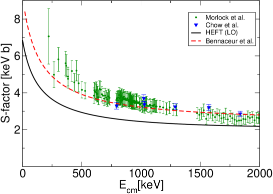
Figure 5: The LO halo EFT result for the astrophysical S-factor for ¹⁶O(p,$\gamma$)¹⁷F${}^{*}(1/2^{+})$ is presented by the solid black line. The theoretical result is compared with the data by Chow et al. [24] and Morlock et al. [25, 26] shown by blue triangles and green dots, respectively. The calculation by Bennaceur et al. [27] is shown by the dashed curve.

Radiative capture into low-lying states of ¹⁷F has been measured by Rolfs et al. [9], Chow et al. [24] and by Morlock et al. [25, 26]. In Fig. 5 we show the astrophysical S-factor, defined as

$$S(E)=E\exp{(2\pi\eta)}\sigma_{\mathrm{tot}}~{}.$$ (30)

The figure shows the halo EFT results of our LO calculation compared to experimental data for capture into the $1/2^{+}$ excited state and a phenomenological calculation using the shell model embedded in the continuum. At threshold, we find that $S(0)\approx 7~{}\mathrm{keV~{}b}$. Our LO results are slightly low, but consistent with the experimental data, within the expected 50% error. We anticipate that the next-to-leading order correction will increase the radiative capture cross section through the appearance of a finite effective range at this order. It can also be noted that the results agree qualitatively with the predictions obtained in the shell model embedded in the continuum [27].

4 Conclusions

In this work, we have shown that Coulomb effects can be included in halo EFT, and that thereby static and dynamical observables of proton halo nuclei become accessible. We have calculated the charge radius and the radiative proton capture cross section of S-wave proton halo nuclei at leading order in halo EFT. Our results can be applied to any one-proton halo system whose interaction is dominated by S-waves. In particular, the excited $1/2^{+}$ state in ¹⁷F is known to have a large S-wave component. We have calculated the charge radius for this system. While this observable is not yet experimentally accessible, this result provides a prediction for ab initio calculations using modern nucleon-nucleon interactions.

In addition, we have compared our results for radiative capture into the excited $1/2^{+}$ state of ¹⁷F with experimental data and found good agreement within the expected error. Furthermore, we found that halo EFT gives the same qualitative behavior for this observable as previous calculations that have employed phenomenological models.

For a quantitative description of the experimental data, higher order corrections are required. In a future publication, we will address how these corrections are included within halo EFT in the presence of Coulomb interactions. The size of these contributions will strongly be affected by the relative size of the effective range and the Coulomb momentum $k_{\mathrm{C}}$, which provides an additional scale in systems with Coulomb interactions. Our calculation is also a first step towards a calculation of properties of ⁸B within halo EFT. This system requires the inclusion of two low-energy constants at leading order since it interacts dominantly in the P-wave [7].

Finally, our approach might prove useful for heavier systems whose static observables can be calculated using ab initio approaches, but for which continuum properties are not accessible within the same framework due to the computational complexity. In this scenario, ab initio predictions of, e.g., the one-proton separation energy could be used to fix the halo EFT parameters, which in turn could be used to predict continuum observables such as the radiative capture cross section. In the case of neutron halos, such an approach was recently carried out to predict novel features in the Calcium isotope chain using halo EFT [28].

References

- [1] M. Thoennessen, B. Sherrill, Nature 473 (2011) 25.
- [2] B. Jonson, Phys. Rep. 389 (2004) 1.
- [3] A. S. Jensen, K. Riisager, D. V. Fedorov, Rev. Mod. Phys. 76 (2004) 215.
- [4] K. Riisager, Phys. Scripta T152 (2013) 014001.
- [5] E. Braaten, H.-W. Hammer, Phys. Rep. 428 (2006) 259.
- [6] H.-W. Hammer, L. Platter, Phil.Trans.Roy.Soc.Lond. A369 (2011) 2679.
- [7] C. Bertulani, H.-W. Hammer, U. van Kolck, Nucl. Phys. A 712 (2002) 37.
- [8] P. F. Bedaque, H.-W. Hammer, U. van Kolck, Phys. Lett. B569 (2003) 159.
- [9] C. Rolfs, Nucl. Phys. A 217 (1973) 29.
- [10] S. Typel, G. Baur, Nucl. Phys. A759 (2005) 247.
- [11] D. L. Canham, H.-W. Hammer, Eur. Phys. J. A 37 (2008) 367.
- [12] H.-W. Hammer, D. R. Phillips, Nucl. Phys. A 865 (2011) 17.
- [13] G. Rupak, R. Higa, Phys. Rev. Lett. 106 (2011) 222501.
- [14] G. Rupak, L. Fernando, A. Vaghani, Phys. Rev. C86 (2012) 044608.
- [15] J. Rotureau, U. van Kolck, Few Body Syst. 54 (2013) 725.
- [16] P. Hagen, H.-W. Hammer, L. Platter, arXiv:1304.6516, to appear in Eur. Phys. J. A (2013).
- [17] B. Acharya, C. Ji, D. R. Phillips, Phys. Lett. B723 (2013) 196.
- [18] R. Higa, H.-W. Hammer, U. van Kolck, Nucl. Phys. A 809 (2008) 171.
- [19] R. Higa, EPJ Web of Conferences 3 (2010) 06001.
- [20] S. Koenig, D. Lee, H.-W. Hammer, J. Phys. G: Nucl. Part. Phys. 40 (2013) 045106.
- [21] X. Kong, F. Ravndal, Phys. Lett. B 450 (1999) 320.
- [22] D. B. Kaplan, M. J. Savage, M. B. Wise, Phys. Rev. C 59 (1999) 617.
- [23] D. Tilley, H. Weller, C. Cheves, Nucl. Phys. A 564 (1993) 1.
- [24] H. C. Chow, G. M. Griffiths, T. H. Hall, Can. J. Phys. 53 (1975) 1672.
- [25] R. Morlock, R. Kunz, A. Mayer, M. Jaeger, A. Müller, J. Hammer, P. Mohr, H. Oberhummer, G. Staudt, V. Kölle, Phys. Rev. Lett. 79 (1997) 3837.
- [26] C. Iliadis, C. Angulo, P. Descouvemont, M. Lugaro, P. Mohr, Phys. Rev. C 77 (2008) 045802.
- [27] K. Bennaceur, F. Nowacki, J. Okołowicz, M. Płoszajczak, Nucl. Phys. A 671 (2000) 203.
- [28] G. Hagen, P. Hagen, H.-W. Hammer, L. Platter, arXiv:1306.3661 (2013).