A Simple Disk Wind Model for Broad Absorption Line Quasars
Abstract
Approximately of quasi-stellar objects (QSOs) exhibit broad, blue-shifted absorption lines in their ultraviolet spectra. Such features provide clear evidence for significant outflows from these systems, most likely in the form of accretion disk winds. These winds may represent the “quasar” mode of feedback that is often invoked in galaxy formation/evolution models, and they are also key to unification scenarios for active galactic nuclei (AGN) and QSOs. To test these ideas, we construct a simple benchmark model of an equatorial, biconical accretion disk wind in a QSO and use a Monte Carlo ionization/radiative transfer code to calculate the ultraviolet spectra as a function of viewing angle. We find that for plausible outflow parameters, sightlines looking directly into the wind cone do produce broad, blue-shifted absorption features in the transitions typically seen in broad absorption line QSOs. However, our benchmark model is intrinsically X-ray weak in order to prevent overionization of the outflow, and the wind does not yet produce collisionally excited line emission at the level observed in non-BAL QSOs. As a first step towards addressing these shortcomings, we discuss the sensitivity of our results to changes in the assumed X-ray luminosity and mass-loss rate, . In the context of our adopted geometry, is required in order to produce significant BAL features. The kinetic luminosity and momentum carried by such outflows would be sufficient to provide significant feedback.
keywords:
galaxies: active - quasars: general - quasars: absorption lines - radiative transfer - methods: numerical1 Introduction
Outflows are key to our understanding of quasi-stellar objects (QSOs) and active galactic nuclei (AGN). First, they are ubiquitous (Ganguly & Brotherton, 2008; Kellerman et al., 1989), suggesting that they are an integral part of the accretion process that fuels the central supermassive black hole (SMBH). Second, they can substantially alter – and in some cases dominate – the observational appearance of QSO/AGN across the entire spectral domain, from X-rays (e.g. Turner & Miller, 2009), through the ultraviolet band (e.g. Weyman et al., 1991), to radio wavelengths (e.g. Begelman, Blandford & Rees, 1984). Third, they represent a “feedback” mechanism, i.e. a means by which the central engine can interact with its galactic and extragalactic environment (King, 2003, 2005; Fabian, 2012).
There appear to be two distinct modes of mass loss from AGN/QSOs: (i) highly collimated relativistic jets driven from the immediate vicinity of the SMBH, (ii) slower-moving, less collimated, but more heavily mass-loaded outflows from the surface of the accretion disk surrounding the SMBH. Intriguingly, both types of mass loss are also seen in other types of accreting systems on all astrophysical scales, such as young stellar objects (YSOs; e.g. Lada, 1985), accreting white dwarfs in cataclysmic variables (CVs; e.g. Körding et al., 2011; Cordova & Mason, 1982) and X-ray binaries containing neutron stars or stellar-mass black holes (e.g. Ponti et al., 2012; Fender, 2006). Thus the connection between accretion and mass loss appears to be a fundamental and universal aspect of accretion physics.
Both jets and winds have been invoked as important feedback mechanisms. The current consensus (e.g. Fabian, 2012) appears to be that winds may dominate feedback during bright QSO phases (the so-called “quasar-mode” of feedback), while the kinetic power of jets may dominate during less active phases (“radio mode”). More specifically, the quasar mode may be responsible for quenching the burst of star formation that characterizes the initial growth phase of a massive galaxy, and thus for moving galaxies from the actively star-forming “blue cloud” to the more passively evolving “red sequence” (Granato et al., 2001; Schawinski, 2007). Conversely, the radio mode appears to be responsible for inhibiting new star formation from taking place via cooling flows in massive red galaxies in the centres of clusters and groups (McNamara & Nulsen, 2007).
Of the two outflow/feedback modes, jets are arguably the better understood, at least phenomenologically. Powerful jets tend to announce their presence via strong radio (and X-ray) emission, and they can often be imaged directly. By contrast, much less is known about the properties of disk winds. This is at least in part due to their much smaller physical size (e.g. Murray & Chiang, 1996), which usually prevents direct imaging studies111Some disk winds in the local universe have been imaged directly. For example, the spatially resolved “ruff” in the radio emission of the classic microquasar SS433 is thought to arise in a disk wind (Blundell et al., 2001).. As a result, the geometry, kinematics and energetics of disk winds typically have to be inferred by indirect means (e.g. Shlosman & Vitello, 1993; Knigge, Woods & Drew, 1995; Arav et al., 2008; Neilsen & Lee, 2009).
Arguably the most direct evidence of disk winds in AGN/QSO is provided by the class of broad absorption line quasars (BALQSOs). These objects make up of the QSO population (Knigge et al. 2008; but also see Allen et al. 2011) and exhibit broad, blue shifted absorption lines and/or P-Cygni profiles associated with strong resonance lines in the ultraviolet (UV) waveband. Such features are classic signatures of outflows and are also seen, for example, in hot stars (e.g. Morton, 1967) and CVs (e.g. Greenstein & Oke, 1982).
In the majority () of BALQSOs, the so-called HiBALs, the observed absorption features are all due to relatively high-ionization species such as C iv, Si iv and N v. In a smaller () sub-set of BALQSOs, the so-called LoBALs, blueshifted absorption is also observed in transitions associated with lower ionization species, such as Mg ii and Al ii. Finally, a small number () of extreme cases, the FeLoBALS, also show absorption in Fe ii and Fe iii.
Intriguingly, these are the same transitions that are typically seen in non-BAL QSOs and AGN, except that here they appear as pure (but still broad) emission lines. Moreover, despite differences in the continuum spectral energy distributions (SEDs), it appears that both BAL and non-BAL QSOs are drawn from the same parent population (Reichard et al., 2003). These considerations have naturally led to the suggestion that the apparent differences between BALQSOs and non-BAL QSOs are merely orientation effects (Elvis, 2000). In such a geometric unification scenario, the “broad emission line region” (BELR) in non-BAL QSOs is a (possibly different) part of the same accretion disk wind that produces the absorption features in BALQSOs. The observational differences between the two classes are then solely due to viewing angle. BAL features are observed when the UV-bright accretion disk is viewed through the outflow, while only BELs are seen when the system is viewed from other directions.
Given the central role played by disk winds in AGN/QSO unification scenarios and galaxy evolution models, it is clearly important to determine the physical properties – i.e. the geometry, kinematics and energetics – of these outflows. However, while there have been many previous efforts in this direction (Murray et al., 1995; Bottorff et al, 1997; Everett, Königl & Karje, 2001; Everett, Königl & Arav, 2002; Proga & Kallman, 2004; Sim, 2005; Schurch & Done, 2007; Schurch, Done & Proga, 2009; Borguet & Hutsemékers, 2010; Giustini & and Proga, 2012), there has not really been a convergence towards a unique physical description. We have therefore embarked on a project to construct a comprehensive, semi-empirical picture of disk winds in AGN/QSO. Our ultimate goal is to test if outflows can account simultaneously for most of the diverse observational tracers of disk winds in AGN/QSOs. The present paper represents the first step in this long-term program. Our aim here is to test if a simple, physically motivated disk wind model can give rise to spectra that resemble those of BALQSOs when the line of sight towards the central engine lies within the wind cone.
The detailed plan of this paper is as follows. In Section 2, we describe the family of kinematic disk wind models we use to describe AGN/QSO outflows. In Section 3, we briefly describe our Monte Carlo ionization and radiative transfer code, python (Long & Knigge, 2002, LK02 hereafter), focusing on the extensions and modifications we have implemented to enable its application to AGN/QSO winds. In Section 4, we discuss observational and theoretical constraints that restrict the relevant parameter space of the model. These considerations allow us to define a benchmark disk wind model as a reasonable starting point for investigating the impact of disk winds on the spectra of AGN/QSO. In Section 5, we present and discuss the synthetic spectra produced by this model. In Section 6, we consider the main shortcomings of the benchmark model and, as a first step towards overcoming them, explore the model’s sensitivity to changes in X-ray luminosity and mass outflow rate. Finally in Section 7, we summarise our findings.
2 The Kinematic Disk Wind Model
Since the driving mechanism, geometry and dynamics of AGN/QSO disk winds are all highly uncertain, we use a flexible, purely kinematic model to describe the outflow. This allows us to describe a wide range of plausible disk winds within a single, simple framework. The specific prescription we use was developed by Shlosman & Vitello (1993, SV93 hereafter) to model the accretion disk winds observed in CVs, i.e. accreting white dwarf binary systems.
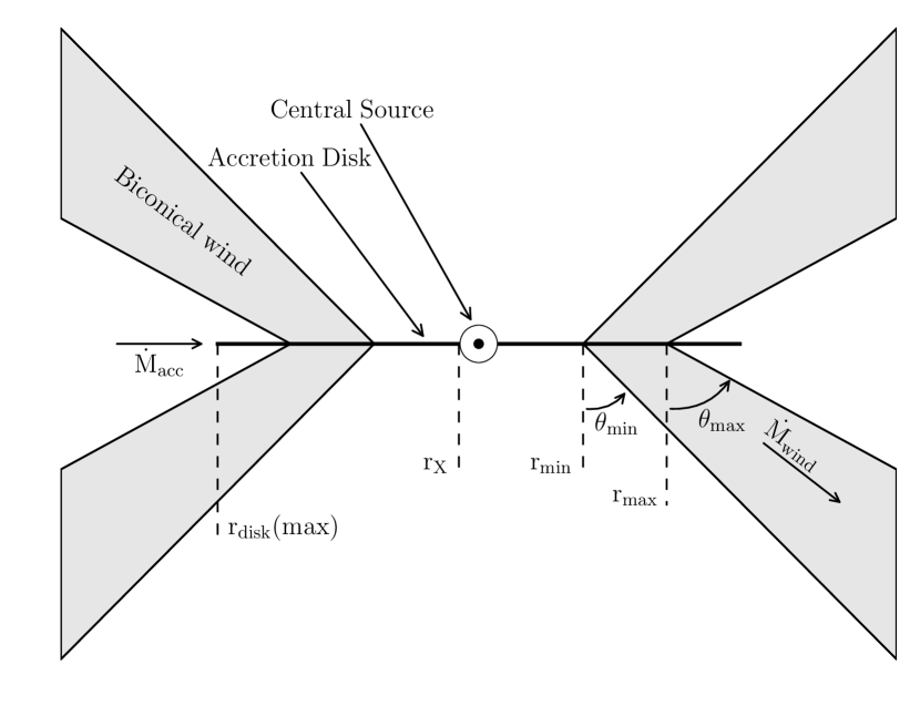
The geometry of our outflow model is illustrated in Figure 1. A biconical wind is taken to emanate between radii and in the accretion disk, with the wind boundaries making angles of and with the axis of symmetry. At each radius, , within this range, the wind leaves the disk with a poloidal (non-rotational) velocity vector oriented at an angle to the axis of symmetry, with given by
| (1) |
where
| (2) |
The parameter can be used to vary the concentration of poloidal streamlines towards either the inner or outer regions of the wind, but throughout this work we fix it to 1, so the poloidal streamlines are equally spaced in radius.
The poloidal velocity, , along a streamline in our model is given by
| (3) |
where is distance measured along a poloidal streamline. This power-law velocity profile was adopted by SV93 in order to give a continuous variation in the derivative of the velocity and a realistic spread of Doppler-shifted frequencies in the outer portion of the wind (. We have similar requirements. The initial poloidal velocity of the wind, is (somewhat arbitrarily) set to for all streamlines, comparable to the sound speed in the disk photosphere. The wind then speeds up on a characteristic scale length , defined as the position along the poloidal streamline at which the wind reaches half its terminal velocity, . The terminal poloidal velocity along each streamline is set to a fixed multiple of the escape velocity at the streamline foot point,
| (4) |
so the innermost streamlines reach the highest velocities. The power-law index controls the shape of the velocity law: as increases, the acceleration is increasingly concentrated around along each streamline. For large , the initial poloidal velocity stays low near the disk and then increases quickly through to values near .
The wind is assumed to initially share the Keplerian rotation profile of the accretion disk, i.e. at the base of the outflow. As the wind rises above the disk and expands, we assume that specific angular momentum is conserved, so that the rotational velocities decline linearly with increasing cylindrical distance from the launch point.
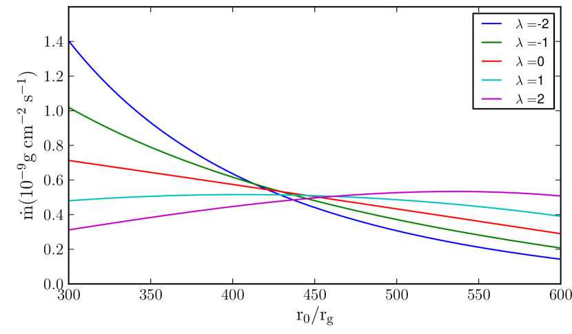
The SV93 prescription also allows us to control the mass loading of the outflow as a function of radius. More specifically, the local mass-loss rate per unit surface area on the disk () is given by
| (5) |
where is the global mass loss rate through the wind. The run of mass loss rate per unit area with is illustrated in Figure 2.
The combination of local mass-loss rate, launching angle and poloidal velocity is sufficient to uniquely determine the density at any point in the wind via a continuity equation (see SV93 for details). The resulting wind is a smooth, single phase outflow without clumps. There is evidence for structure in BALQSO outflows, apparent from complex line shapes (e.g. Ganguly at al., 2006; Simon & Hamann, 2010) and time variability (e.g. Capellupo et al., 2011, 2012, 2013), but this is something our simple model cannot address. However, hot star winds and CV winds also exhibit variability and small-scale structure, yet much has been learned about these winds by focussing on the global, underlying smooth flow field. This is the approach followed here.
3 Ionization, Radiative Transfer and Spectral Synthesis
In order to calculate the spectra predicted to emerge from our disk winds, we use python, a radiative transfer code designed to model biconical outflows and first described by LK02. The code has been used previously to calculate model spectra for disk-dominated CVs (Noebauer et al., 2010) and young stellar objects (Sim et al., 2005). Here, we provide a brief overview of the code, focussing particularly on the modifications we have made recently to enable modelling of BALQSOs. All simulations shown in this paper were carried out with version 75 of python.
3.1 Basic Structure
python is a hybrid Monte Carlo/Sobolev radiative transfer code that works by following the progress of energy packets through a simulation grid of arbitrary size, shape and discretization. For the simulations described here, we utilize an azimuthally symmetric cylindrical grid. Energy packets are characterized by a frequency and a weight, defined so that the sum of all packets correctly represents the luminosity and spectral energy distribution of all radiation sources in the model.
The thermal and ionization structure of a wind model is computed iteratively through a series of ‘ionization cycles’. During each cycle, energy packets are tracked through the wind and their effect on the wind’s temperature and ionization state is computed (see Section 3.3 below). Once the ionization structure of the wind has been determined, a series of ‘spectral cycles’ are executed, in which synthetic spectra are generated at specific inclination angles.
3.2 Radiation Sources
For simulations of AGN/QSO, the radiative sources included are a central X-ray source, an accretion disk and the wind itself. We assume that the central source produces a power-law SED and that the optically thick, geometrically thin disk radiates as an ensemble of blackbodies. We do not at present apply the colour temperature correction as suggested in Done et al. (2012) but the correction is in any case modest for the accretion disk in our benchmark model.
The geometry of the X-ray emitting region in AGN is not fully understood, but the emission is believed to arise from a hot corona above the inner regions of the accretion disk (e.g. Galeev, Rosner & Vaiana, 1979). Here, we follow Sim et al. (2008) and assume the central X-ray source is an isotropically radiating sphere, with radius equal to the innermost radius of the accretion disk (typically set to , the radius of the innermost circular stable orbit [ISCO] for a non-rotating black hole). The X-ray source produces energy packets governed by a power law in flux, i.e.
| (6) |
where is the spectral index. In practice, we characterize the X-ray source primarily by its integrated luminosity between 2-10 keV, which is related to and via
| (7) |
UV continuum emission in AGN is thought to be dominated by an accretion disk. We assume the disk has the radial temperature profile of the standard thin disk equations (Shakura & Sunyaev, 1973), i.e.
| (8) |
where
| (9) |
Here, is the accretion rate through the disk, and we take , appropriate for a non-rotating SMBH.
Finally, the wind itself is a hot thermal plasma and therefore radiates through various atomic processes including line emission, recombination and/or free-free processes. Unlike the other radiation sources, the radiation field produced by the wind has to be computed iteratively, since it depends on the ionization state and temperature of the outflow. The wind is always assumed to be in radiative equilibrium, i.e. it reprocesses radiation originally produced by the disk and the central source. These components therefore set the total luminosity of the system – the wind is not a net source of photons in our model. 222In principle, it would be simple to allow for non-radiative energy input into the wind (e.g. shocks or energy release via magnetic reconnection events). However, the relevance of these processes, let alone the detailed form they would take, is presently unknown.
3.3 Thermal and Ionization Equilibrium
3.3.1 Overall Iteration Scheme
At the beginning of each simulation, the electron temperature () and ionization state of the wind are initialized by assuming a reasonable value for and adopting LTE ionization fractions. As the energy packets progress through the wind, they lose energy via continuum and line absorption, thereby heating the wind. They can also change frequency in the observer frame via scattering in the outflowing wind. However, since such scattering events are assumed to be coherent in the comoving frame, these frequency changes do not contribute to heating.
As energy packets move through the wind, all of the quantities that are needed to calculate the ionization are logged. These include the frequency-integrated mean (angle-averaged) intensity (), the mean frequency () and the standard deviation () of the frequency of energy packets passing through the cell. These quantities are logged in a series of frequency bands to provide information for the ionization calculations described below. We also calculate ‘global’ values for these quantities (integrated over the entire frequency range) in each cell, for use in the heating and cooling calculations. All energy packets are tracked until they escape the wind.
After each cycle in the ionization stage, a new estimate of is computed via a process of minimising the absolute value of the difference between , the heating rate computed during the cycle, and , the cooling rate which is expressed as a function of . The code then recomputes the ionization state of the wind, using the new estimate of the temperature and the information recorded about the radiation field in the cell. In order to improve the stability of the code, we restrict the amount by which can change in one ionization cycle.
Armed with new estimates of electron temperature and ionization state, the code then starts the next ionization cycle. This iteration proceeds until the electron temperature in each cell has converged to a stable value. At this point, all physical parameters of the wind are frozen, and synthetic spectra can be produced for any desired wavelength range or inclination angle.
3.3.2 Ionization Balance
LK02 determined the ionization state of the wind using a “modified on-the spot approximation” first derived by Abbot & Lucy (1985). This treatment is designed for a situation in which the local radiation field is fairly close to a dilute blackbody, as is the case for O-star winds and CVs. However, unlike O stars and CVs, AGN/QSO emit a significant fraction of their energy in X-rays and have global SEDs that are poorly described by blackbodies.
We have therefore implemented a new method to calculate the ionization state of the wind into python, which is better suited to situations in which relatively soft (UV) and relatively hard (X-ray) components both contribute significantly to the ionizing radiation field. Our new ionization treatment follows that described by Sim et al. (2008), which can be summarized by the ionization equation
| (10) |
Here, is the electron density and represents the density of the ground state of ionization stage of a particular atomic species. The quantity is the ratio computed via the Saha equation at temperature , while is the fraction of recombinations going directly into the ground state, allowing for both radiative recombinations into all levels and dielectronic recombinations. The correction factor is the ratio of the photoionization rate expected for the actual SED to that which would be produced by a blackbody at ,
| (11) |
Here, is the frequency-dependent photoionization cross-section for ionization state , and is the monochromatic mean intensity.
This formulation allows us to correctly account for the photo-ionizing effect of radiation fields with arbitrary SEDs, provided there are sufficient photon packets to adequately characterise the SED. In this work, we model the SED in each cell after each ionization cycle by splitting it into a series of user-defined bands. Equation 11 can then be re-written as
| (12) |
where the summation in the numerator is now over bands, each running over a frequency range . In practice, the monochromatic mean intensity in each band is modelled as either a power law,
| (13) |
or an exponential
| (14) |
The values for the four parameters , , and , are deduced from the two band-limited radiation field estimators mentioned in Section 3.3.1, i.e. and . Thus, for each model, the two free parameters are set by requiring that integrating and over frequency yields the correct values for and . The choice between the exponential and power-law models is finally made by comparing the third band-limited estimator of the radiation field, , to the value predicted by each model.
3.3.3 Heating and cooling
Earlier versions of python accounted for heating and cooling due to free-free, free-bound and bound-bound processes, as well as for adiabatic cooling due to the expansion of the wind. For this study, we have added Compton processes and dielectronic recombinations to the heating and cooling processes included in the code. The former, especially, can be important in QSO winds.
Compton Heating and Cooling
Following Sim et al. (2010), we calculate the Compton heating rate in a cell with electron density as
| (15) |
where the summation is carried out over all photon packet paths of length in the cell. Each photon packet carries luminosity (weight) and has frequency . Here, is the mean energy lost per interaction, equal to averaged over scattering angles. The Klein-Nishina formula is used to compute the cross section .
We also include induced Compton heating in our calculations. Following Cloudy & associates (2011), we estimate this heating rate as
| (16) |
where is the photon occupation number given by
| (17) |
Finally, the Compton cooling rate () is given by
| (18) |
where is the volume of the wind cell.
Dielectronic Recombination Cooling
At the high temperatures expected in a wind irradiated by X-ray photons, dielectronic recombinations can become a significant recombination channel. Even though the associated energy loss from the plasma is never a major cooling process, we include it in our calculations to maintain internal consistency (i.e. processes affecting both ionization and thermal equilibrium should be represented in both calculations). We estimate the cooling rate due to dielectronic recombinations as
| (19) |
where is the temperature-dependent dielectronic recombination rate coefficient for each ion in a cell. The main approximation made in this equation is that the energy removed from the electron pool per dielectronic recombination is equal to the mean kinetic energy of an electron ().
3.3.4 Code Validation
In order to validate the design and implementation of our ionization algorithm, we have carried out a series of tests against the well-known photoionization code cloudy (Ferland et al., 2013). In these tests, we consider a geometrically thin spherical shell illuminated by a wide range of input SEDs, including specifically SEDs with significant X-ray power-law components. We generally find good agreement between the ionization states predicted by python and cloudy in these tests for species important in the BAL context. We also find good agreement in the predicted electron temperatures for quite a wide range of models.
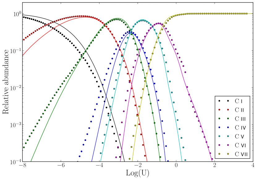
One example of these tests is shown in Figure 3. Here, we plot the relative abundances of the various ionization stages of carbon as a function of ionization parameter
| (20) | |||||
| (21) | |||||
| (22) |
where is the number of hydrogen-ionizing photons emitted by the illuminating source per second, is the distance to the source, is the local hydrogen number density and is the speed of light. is the monochromatic luminosity. The ionization parameter is a measure of the ratio of the ionizing photon density and the local matter density. As such, it is a good predictor of the ionization state of optically thin photoionized plasmas.
In the test shown in Figure 3, the irradiating SED was modelled as a a doubly-broken power law with below eV, above keV and between these break frequencies. This was in order to allow direct comparison with a cloudy model defined via the power law command. The spherical shell was assumed to lie at cm, the hydrogen density was taken to be and the ionization parameter was adjusted by varying the luminosity of the ionizing SED. With such a simple set-up, both the SED and the geometry can be modelled in exactly the same way in both python and cloudy. Given the likely differences in detailed atomic physics and atomic data used in cloudy and python, there is good agreement between the codes, especially for the moderately to highly ionized stages of carbon that we expect to see in the vicinity of a QSO. This agreement is illustrated in Figure 3.
As noted above, the electron temperatures predicted by python and cloudy also generally agree quite well. One exception to this is situations in which iron lines dominate the cooling, where python can overestimate the temperature by as much as a factor of about 2. Some wind regions in our benchmark model are likely to be affected by this. However, since the electron temperature only appears in the ionization equation via , the effect of this issue on the relevant ionization fractions in our models is relatively small.
3.4 Spectral Synthesis
Once the thermal and ionization state of the wind has converged, the ionization cycles are terminated and the spectral cycles begin. In the latter, the thermal and ionization structure are considered fixed, and photons are only generated over the restricted frequency range for which detailed predictions are needed. This saves CPU time and allows us to achieve much greater spectral resolution and signal-to-noise in the simulated spectra.
The spectra themselves are extracted from the Monte Carlo simulation using the techniques described by LK02. Collisionally excited line emission is treated in the two-level atom approximation, which is acceptable for strong resonance lines in which the upper level is populated by transitions from the lower (ground) state. Most of the transitions associated with BALs and BELs fall into this category. However, this approximation is not adequate for many other transitions, most notably the Hydrogen Lyman and Balmer series, for which the upper states are populated by a radiative recombination cascade. (Sim et al., 2005) have already used a more general method to model infrared Hi line emission in YSOs with python; work is in progress on implementing this treatment into our simulations of AGN/QSOs.
3.5 Atomic data
For the calculations described in this paper, we include atomic data for H, He, C, N, O, Ne, Na, Mg, Al, Si, S, Ar, Ca and Fe. Elemental abundances are taken from Verner, Barthel & Tytler (1994) and the basic atomic data, such as ionization potential and ground state multiplicities, are taken from Verner, Verner & Ferland (1996). For H, He, C, N, O and Fe, we use topbase (Cunto et al., 1993) data for energy levels and photoionization cross sections from both ground state and excited levels. For other elements, we use the analytic approximations for ground state photoionization cross sections given in Verner, Ferland, Korista & Yakovlev (1996). For bound-bound transitions, we use the line list given in Verner, Verner & Ferland (1996), which contains nearly 6000 ground-state-connected lines. The levels associated with these lines are computed from the line list information using a method similar to that described by Lucy (1999).
We adopt dielectronic recombination rate coefficients and total radiative rate coefficients from the chianti database version 7.0 (Dere et al., 1997; Landi et al., 2012). Ground state recombination rates are taken from Badnell (2006) where available and otherwise computed from the photoionization data via the Milne relation. Finally, we use Gaunt factors for free-free interactions given by Sutherland (1998).
4 A Benchmark Disk Wind Model For BALQSOs
One of the main challenges in trying to model BALQSOs is that the physical characteristics of the disk winds that produce the BALs are highly uncertain. The kinematic model described in Section 2 is sufficiently flexible to describe a wide range of outflow conditions, but the price for this flexibility is a potentially huge parameter space. We have therefore used a variety of theoretical and observational constraints (and considerable trial and error) to design a benchmark disk wind model whose predicted spectrum resembles that of a BALQSO (for sightlines cutting through the outflow).
Since we have not yet carried out a systematic exploration of the relevant parameter space, we make no claim that this fiducial model is optimal, nor that it faithfully describes reality. Indeed, in Section 6, we will discuss some of its shortcomings. However, we believe it is nevertheless extremely useful as a benchmark. More specifically, it provides (i) a first indication of what can be realistically expected of disk wind models; (ii) a better understanding of the challenges such models face; (iii) a convenient starting point for further explorations of parameter space.
In the rest of this section, we will discuss the constraints that have informed our choice of parameters for the benchmark model, which are summarised in Table 1.
4.1 Basic Requirements: BALnicity and Ionization State
Our primary aim here is to find a set of plausible parameters for a QSO wind that yield synthetic spectra containing the features expected of a BALQSO from a range of viewing angles. As noted in Section 1, in the majority of BALs, the HiBALs, the absorption features are due to highly ionized species such as N v 1240, C iv 1550, and Si iv 1400. The C iv feature, in particular, is most often used to identify BALQSOs, so we judge the initial success of candidate wind models by their ability to produce this feature. In practice, this is primarily a constraint on the ionization state of the wind: we require that C iv should be present – if not necessarily dominant – throughout an appreciable fraction of the outflow.
BALs are usually identified via the so-called BALnicity index (BI) (Weyman et al., 1991), which is a measure of absorption strength in the velocity range between and . It is therefore not sufficient to produce C iv anywhere in the outflow – in order for the model to resemble a BAL, C iv needs to be present in reasonable concentrations in regions characterized by the correct velocities.
4.2 Black Hole Mass, Accretion Rate and Luminosity
Our goal is to model a fairly typical, high-luminosity (BAL)QSO, so we adopt a black hole mass of , along with an Eddington ratio of . For an assumed accretion efficiency of , this corresponds to an accretion rate of and a bolometric disk luminosity of .
4.3 Outflow Geometry
BALQSOs represent of all QSOs (e.g. Knigge et al. 2008; Hewett & Foltz 2003, but also see Allen et al. 2011). There are two obvious ways to interpret this number: (i) either all QSOs spend of their life as BALQSOs (“evolutionary unification”; e.g. Becker et al. 2000), or (ii) all QSOs contain disk winds, but the resulting BAL signatures are visible only from of all possible observer orientations (“geometric unification”; e.g. Elvis 2000).333This could be an underestimate, since intrinsic BALQSO fractions tend to be derived from magnitude-limited samples, with no allowance for the possibility that foreshortening, limb-darkening or wind attenuation may reduce the continuum flux of a typical BALQSO relative to that of a typical QSO (Krolik & Voit, 1998). For the purpose of the present paper, we ignore this potential complication. Here, we adopt the geometric unification picture, with the aim of testing its viability.
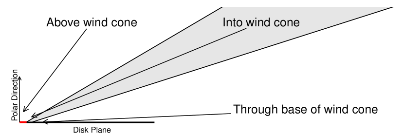
As illustrated in Figure 4, our wind geometry allows for three distinct classes of sightline towards the central engine. Looking from the polar direction, “above the wind cone”, the sightline does not intersect the wind at all, and looking from the equatorial direction, the sightline passes through the base of the wind cone where the projected line of sight velocities are too low to produce BAL features. We anticipate that BAL features will result when the central engine (or, strictly speaking, the UV-bright portions of the accretion disk) are viewed from the third class of sightline - looking “into the wind cone”. We therefore expect such sightlines to subtend 20% of the sky as seen by the central engine. Note that this description of the sightlines only applies to models like our benchmark model, in which most of the emission arises from inside the wind launching radius.
If we define and as the angles made by the inner and outer boundaries of the wind with respect to the disk normal, these constraints translate into a simple relationship between and , i.e.
| (23) |
Most geometrical unification scenarios assume that BAL-producing QSO winds flow predominantly along the equatorial plane of the disk, rather than along the polar axis (e.g. Weyman et al. 1991; Ogle et al. 1999; Elvis 2000; however, see Zhou et al. 2006 and Brotherton, De Breuck & Schaefer 2006 for a contrary view). In line with this general view, we have found that ionization states capable of producing C iv and other typical BAL features are more naturally produced in equatorial, rather than polar disk winds. This is because one of the main challenges faced by disk wind models is to prevent the over-ionization of the outflow by the central X-ray source (see below). Other things being equal, equatorial winds are less ionized, partly because of limb darkening, and partly because the disk appears foreshortened from equatorial directions. In addition, in geometries like ours, where the wind arises from parts of the disk radially outside the location where the ionizing radiation is produced, an equatorial wind exhibits self-shielding, i.e. the radiation must pass through the inner parts of the wind to reach the outer parts. Therefore the ionization state can be lower than for a polar wind, where all parts of the wind can see the ionizing radiation directly.
Based on these considerations, we adopt a mostly equatorial geometry with and for our benchmark model. With this choice, 66% of the remaining sightlines lie “above” the wind cone, while 14% view the central source through the base of the wind. If geometric unification is correct and complete – in the sense that the emission lines in non-BAL QSOs are produced by the same outflow that produces the absorption features seen in BALQSOs (e.g. Elvis, 2000) – we would ideally see different classes of QSO as we view a given system from the three distinct types of viewing angles.
4.4 Wind-Launching Region
There is no consensus on the location of the wind-launching region on the accretion disk. However, there are several empirical and theoretical considerations that can inform the design of our benchmark model.
First, within the geometric unification scenario, QSO disk winds are responsible not only for BAL features, but also for the broad emission lines (BELs) seen in non-BAL QSOs. We can therefore use the result of reverberation mapping studies of this broad line region (BLR) to guide us in locating the outflow. Kaspi et al. (2000) have carried out reverberation mapping of the C iv BLR for high luminosity quasars. A representative example is S5 0836+71, a quasar with a black hole mass of , for which they found a rest frame delay of 188 days. This implies a distance of the line-forming region from the UV continuum source of .444Note that the UV continuum is produced at very small radii compared to the wind launch radius and so can be treated as originating from the centre of the model for these estimates Since the C iv line-forming region may lie substantially downstream in the outflow, this is an upper limit on the distance of the launching region from the centre.
Second, BAL features exhibit variability on timescales from days to years (e.g. Capellupo et al., 2011, 2012, 2013). If interpreted in terms of wind features crossing our line of sight, the shortest variability time scales – which arise in the innermost parts of the line-forming region – correspond to distances of cm or, equivalently, from the centre (for an assumed ).
Third, one of the most promising mechanisms for driving QSO disk winds is via radiation pressure in spectral lines (e.g. Proga, Stone & Kallman, 2000; Proga & Kallman, 2004). Empirical support for this idea comes from the presence of the “ghost of Lyman ” in some N v BAL features (see Arav et al. 1995; Arav 1996; North, Knigge & Goad 2006; but also see Cottis et al. 2010). In published simulations where such winds are modelled in a physically consistent manner, the typical launching radii are (e.g. Proga, Stone & Kallman, 2000; Risaliti & Elvis, 2010).
Fourth and finally, it is physically reasonable to assume that the maximum velocity achieved by the outflow corresponds roughly to the fastest escape velocity in the wind launching region on the accretion disk. Observationally, , which, for a black hole, corresponds to the escape velocity from .
Taken together, all of these considerations suggest that a reasonable first guess at the location of the wind-launching region on the disk is on the order of a few hundred . In our benchmark model, we therefore adopt and .
4.5 Wind Mass-Loss Rate
One of the most fundamental parameters of any wind model is the mass-loss rate into the outflow, . In our benchmark model, we set . This value was arrived at mainly by trial and error, but with a conservative preference for values satisfying . As shown explicitly in Section 6.1, in practice, we found that we required in order to produce BAL features for even modest X-ray luminosities.
Strictly speaking, any model with is not entirely self-consistent, since the presence of such an outflow would alter the disk’s temperature structure (e.g. Knigge, 1999). However, we neglect this complication, since the vast majority of the disk luminosity arises from well within our assumed wind-launching radius. Thus even though our model ignores that the accretion rate is higher further out in the disk, it correctly describes the innermost disk regions that produce virtually all of the luminosity.
4.6 Velocity Law Parameters
Ideally, the parameters defining the poloidal velocity law of the wind would be predicted by the relevant acceleration mechanism. However, since this is not yet possible, we have simply adopted parameters that result in reasonably BAL-like C iv features.
As noted in Section 4.4 above, it seems physically plausible that the terminal outflow velocity along a poloidal streamline will roughly reflect the local escape velocity at the streamline footpoint. Having already adopted wind launching radii based on this idea, we therefore also adopt , i.e. in Equation 4.
The other two parameters defining the poloidal velocity law are , the poloidal distance at which the velocity is equal to half the terminal velocity, and , the exponent describing how the velocity varies with poloidal distance. As discussed above, the locations of BAL- and BEL-forming regions within the wind likely extend to distances of up to about , so this is a reasonable number to adopt for . For the black hole in our benchmark model, this corresponds to cm. Finally, in the absence of other information, we adopt . This produces a relatively slow acceleration as a function of poloidal distance along a streamline and seems to produce reasonable BAL shapes. We will explore the effect of changing these parameters in future work.
4.7 X-ray Spectrum and Luminosity
The X-ray luminosity of the central source is set to in our benchmark model. This value was arrived at through the requirement that the model should produce BALs which constrains the X-ray luminosity, since X-rays can strongly affect the ionization state of the outflow. We set the spectral index of the X-ray spectrum to , as suggested by Giustini, Cappi & Vignali (2008).
Quasar spectra are often characterised in terms of the ratio of X-ray to bolometric (or UV) luminosity. This ratio is usually characterized by the spectral index between X-rays and optical/UV, , defined as
| (24) |
where and are the inferred monochromatic luminosities at 2 keV (X-ray) and 2500 Å(UV), respectively. Ignoring the angle dependence of the disk emission, we obtain a mean value of for the parameters used in our benchmark model. This is considerably lower than observed in typical non-BAL QSOs (Just et al., 2007) and lies near the lower (X-ray weak) end of the range of seen in BALQSOs (e.g Giustini, Cappi & Vignali, 2008; Gibson et al., 2009). The X-ray weakness of the model, as well as the sensitivity of our results to the adopted X-ray luminosity, are discussed in more detail in Section 6.1.
4.8 Size and Resolution of the Numerical Grid
The outer edge of our simulation grid is set to . This is large enough to ensure that all spectral features of interest arise entirely within the computational domain. In all simulations shown in this paper, this domain is sampled by a cylindrical grid composed of logarithmically spaced cells. We have carried out resolution tests to ensure that this is sufficient to resolve the spatially varying physical conditions and ionization state of the outflow.
| Free Parameters | Value |
|---|---|
| (f=1) | |
| cm | |
| Derived Parameters | Value |
| -27.4 | |
| -26.2 | |
| -2.2 |
5 Results and Analysis
Having defined a benchmark disk wind model for AGN/QSOs, we are ready to examine its predicted physical and observable characteristics. In Section 5.2 we will present synthetic spectra reminiscent of BALQSOs for sightlines looking into the wind cone. However, it is helpful to examine the physical and ionization state of the benchmark model before analyzing these spectra in detail.
5.1 The Physical State of the Outflow
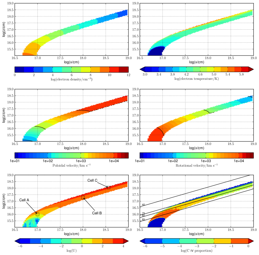
The top four panels in Figure 5 show a selection of physical parameters of the converged wind model. Considering first the electron density (top left panel), we see that our choice of kinematic parameters has given rise to an outflow with a fairly high density of at its base. However, this declines quickly as we move outwards, due to the expansion and acceleration of the wind. Hydrogen is fully ionized throughout the entire outflow, so everywhere.
The electron temperature in the wind ranges from near the base of the wind to more than (top right panel). The highest temperatures are in a thin layer near the “top” of the wind, at distance of from the central engine. These regions are hot because they are directly exposed to the radiation field of the accretion disk and the X-ray source. These regions also shield the wind material “behind” them, however, and thus help to ensure more moderate temperatures in the rest of the outflow. In fact, much of the disk wind is heated to temperatures near , which are quite conducive to the formation of the high-ionization lines typically seen in (BAL)QSOs, such as C iv, Si iv and N v.
The middle panels of Figure 5 illustrate the velocity structure of our benchmark model, separated into poloidal (middle left panel) and rotational (middle right panel) components. The poloidal velocities show the relatively gradual speed-up of the outflow as a function of distance, which is due to our choice of velocity law exponent. As one would expect, low velocities are found near the base of the wind and high velocities are reached only quite far out. It is this variation in poloidal velocity which produces BAL features as photons produced by the effectively point-like central UV source are scattered out of the line of sight by progressively faster moving wind parcels.
By contrast, the highest rotational velocities are found near the disk plane, where they are effectively equal to the Keplerian velocities in the disk. They then decline linearly with increasing cylindrical distance from the rotation axis, because we assume that wind material conserves specific angular momentum. The projected rotational velocity along a sightline to the central source is zero (or nearly so), and therefore rotational velocities do not play a major part in the formation of BAL features, although they should help in producing broad emission lines.
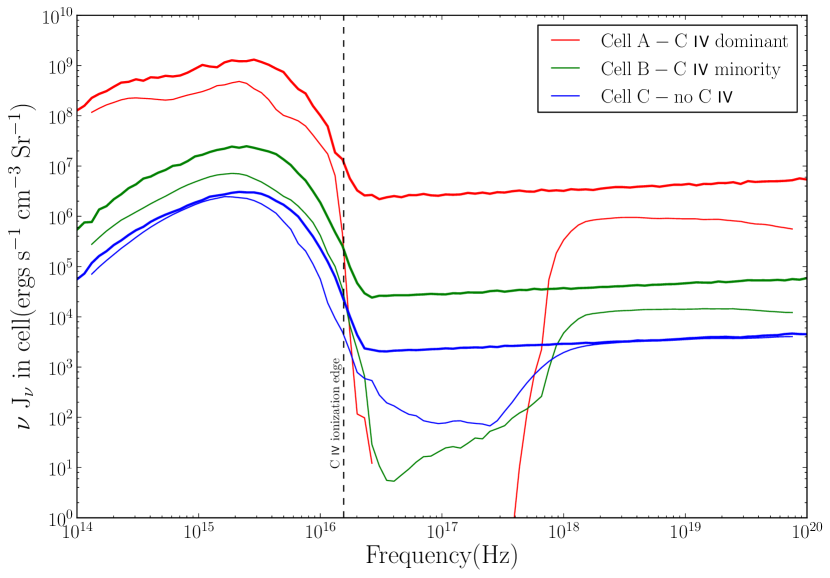
The bottom left and right panels in Figure 5 show the ionization parameter and C iv ionization fraction throughout the outflow, respectively. Interestingly, the model generates sufficient concentrations C iv to make strong BALs even though throughout most of the wind. This contrast with the results shown for a thin-shell model in Figure 3, where this ion is not present for such values of . The main reason for this difference is that the wind is self-shielding: absorption in the inner parts of the outflow (primarily due to photoionization) can strongly modify the SED seen by the outer parts of the wind. This, in turn, changes the ionization parameter at which particular ions are preferentially formed. Figure 6 illustrates the effect of the self-shielding on the SED seen by different parts of the outflow.
5.2 Observing the Model: Synthetic Spectra
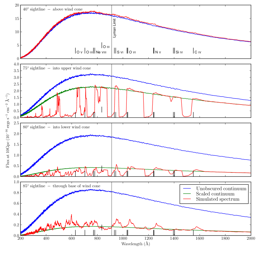
Figure 7 shows the spectra we predict for observers located along the directions indicated in the lower right panel of Figure 5. These viewing angles correspond to sightlines to the central source that look above the wind cone (), into the wind cone ( and ), and through the base of the wind cone (). For comparison, we also show a pure, unobscured continuum spectrum for each viewing angle; these continua were generated by re-running the model with the wind density set to a negligible value.
5.2.1 Sightlines looking into the wind cone
The two middle panels in Figure 7 show the emergent spectra for sightlines through the wind ( and ). These spectra clearly contain BALs, i.e. broad, blue-shifted absorption features associated with several strong, high-ionization lines in the UV region. More formally, we calculate BIs of () and () for the C iv lines we predict for these two sightlines. Thus observed systems displaying these spectra would certainly be classified as bona-fide BALQSOs. This is one of the main results of our work.
Many of the transitions exhibiting BAL features in the spectra for both sightlines also show a redshifted emission component, forming the other part of the classic P-Cygni profile seen in such sources. This can be interpreted as the red-shifted part of a classic rotationally broadened, double-peaked emission line, which is produced primarily by scattering in the base of the wind. The blue-shifted part of the line profile is not visible, since it is superposed on and/or absorbed by the BAL feature.
Another interesting feature of the BAL spectra is that the Si iv absorption feature is narrower than the C iv feature for all sightlines. This is due to the lower ionization potential of the silicon ion, meaning that it is produced in a more limited part of the wind. The relative strengths of features is broadly in agreement with observations (Gibson et al., 2009) and demonstrates that, at least to first order, we are predicting the correct ionization state in the BAL-forming portion of the wind.
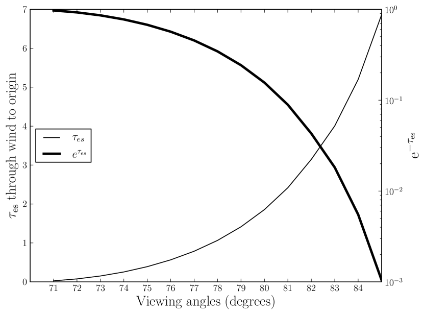
The continuum for both sightlines through the wind is suppressed relative to the unobscured SED (see Figure 7). This attenuation of the continuum is predominantly due to electron scattering. The optical depth to electron scattering through the wind is shown in Figure 8, along with the corresponding attenuation factor, . For example, at our model gives and , in agreement with Figure 7.
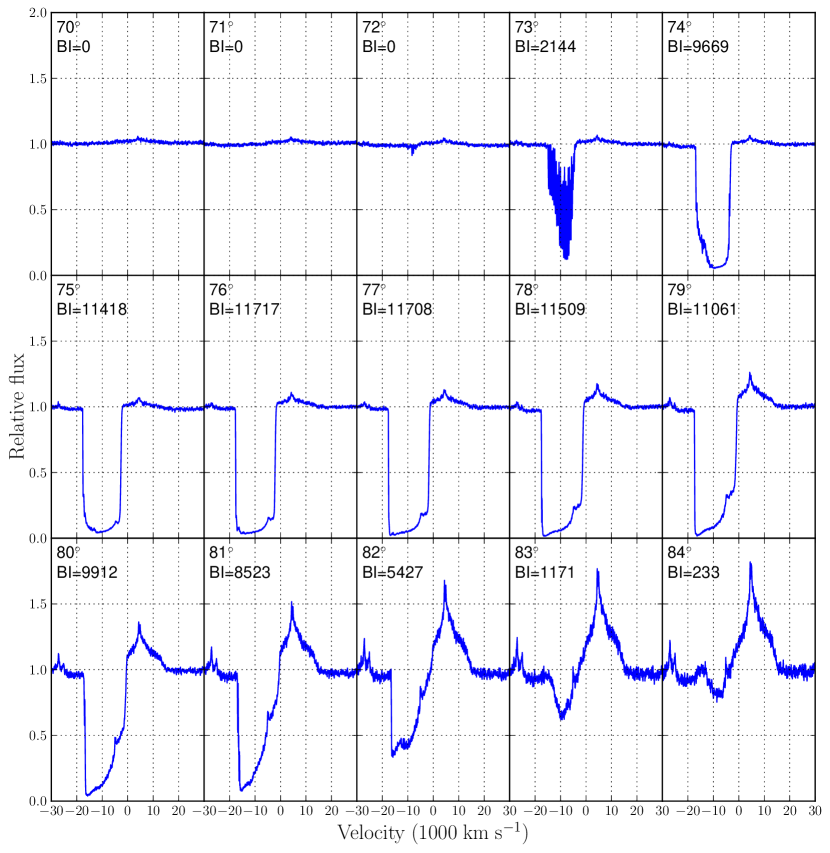
Detailed C iv line profiles predicted by our model for a more finely spaced grid of sightlines are shown in Figure 9, along with the calculated for each profile. BALs (i.e. features with ) are observed for inclinations , which represents of all possible sightlines.
5.2.2 Sightlines looking above the wind cone
We now consider the sightline, which views the central engine from “above” the wind cone. In a pure geometric unification scenario, this sightline may be expected to produce a classic Type I QSO spectrum. What we observe from the simulation is a slightly enhanced continuum, along with some broad, but weak emission lines (as in Sim et al. (2008)).
The continuum enhancement is mainly due to electron scattering into this line of sight. As we have seen in Section 5.2.1 and Figure 8, the base of the wind is marginally optically thick to electron scattering in directions along the disk plane. Thus photons scattering in this region tend to emerge preferentially along the more transparent sightlines perpendicular to this plane, and the wind essentially acts as a reflector.
More importantly, the emission lines superposed on the continuum do correspond to the typical transitions seen in Type I QSOs, but they are weaker than the observed features. For example, the C iv emission line in our model has an equivalent width of only 1.4 Å. By contrast, the equivalent with of the C iv line in a typical QSO with a continuum luminosity of is Å (Xu et al., 2008). Other sightlines above the wind cone () yield qualitatively similar spectra. Overall, the presence of the right “sort” of emission lines is encouraging, but their weakness is an obvious shortcoming of the model. We will discuss the topic of line emission in more detail in Section 6.2.
5.2.3 Sightlines looking through the base of the wind cone
Let us finally consider the highest inclinations, which correspond to sightlines that do not lie along the wind cone, but for which the UV continuum source (i.e. the central region of the accretion disk) is viewed through the dense, low-velocity base of the outflow. It is not obvious what type of QSO one might expect to see from such sightlines, since in the standard model of QSOs, one might expect the torus to obscure such sightlines.
Figure 8 shows that the for this inclination, and indeed we find that essentially all of the radiation emerging from the model in this direction has been scattered several times within the wind before ultimately escaping along this vector. This is in line with results presented by Sim et al. (2010), who found that, for Compton-thick winds, AGN spectra at high inclination are dominated by scattered radiation. Recent observational work (e.g. Treister, Urry & Virani, 2009) has demonstrated that there is a population of AGN in the local universe where the X-ray source is completely obscured, and the X-ray spectrum is dominated by reflection. These high inclination sightlines could represent these so called “reflection dominated Compton thick AGN”.
The shape of the predicted emission features is dominated by the rotational velocity field in the wind. Taking C iv as an example and examining Figure 5, we see that the fractional abundance peaks in a region where the rotational velocity is significantly higher than the outflow velocity. Scattering from this region (along with any thermal emission) will produce the double-peaked line profile that is characteristic of line formation in rotating media (e.g. Smak, 1981; Marsh & Horne, 1988). The blue part of this profile is then likely suppressed, since it is superposed on and/or absorbed by blue-shifted absorption in the base of the wind.
6 Discussion
The results shown in the previous section confirm that a simple disk wind model can produce the characteristic BAL features seen in about of QSOs. However, they also reveal some significant shortcomings of the model. In this section, we will consider some of the key questions raised by our results in more detail and point out promising directions for future work.
6.1 The Sensitivity of BAL Features to X-ray Luminosity
As noted in Section 4.7, our benchmark model is rather X-ray weak compared to most real (BAL)QSOs. To quantify this, Figure 10 shows the viewing angle dependence of for our benchmark model. Clearly, (i.e. the X-ray to optical ratio) is a strong function of inclination. Two effects are responsible for this.
First, the UV and optical fluxes are dominated by the accretion disk and thus decline steeply with inclination, due to foreshortening and limb-darkening. By contrast, the X-ray source is assumed to emit isotropically (although the disk can obscure the “lower” hemisphere). Thus, in the absence of any outflow, increases with inclination, as the X-rays become relatively more important. This is the trend marked by the solid line in Figure 10.
Second, sightlines to the central engine that cross the wind cone can be affected by absorption and radiative transfer in the outflow. In particular, bound-free absorption preferentially suppresses the X-ray flux along such sightlines in our model, and hence reduces . The crosses in Figure 10 show the predicted values of taking both effects into account. This shows that the suppression of is strongest for sightlines looking directly into the wind, i.e. the same viewing angles that produce BALs.
For our benchmark model, we find that for and for . If these viewing angles can be taken to represent non-BAL QSOs and BALQSOs respectively, we can compare these values to those expected from the observed scaling relation between and found by Just et al. (2007) for non-BAL QSOs,
| (25) |
Taking the values of for the two sightlines from our benchmark model, we obtain empirical predictions of for and for . However, we still have to correct for the fact that BALQSOs are known to be X-ray weak (presumably due to absorption in the outflow). Gibson et al. (2009) find that the median for all BALQSOs with , but the distribution of is quite wide, and systems with large tend to have larger . If we adopt as typical for strong BALQSOs (like our benchmark model), the empirically predicted value for the BALQSO sightline becomes (where the quoted uncertainty is purely that associated with the scaling relation for non-BAL QSOs).

These numbers make the X-ray weakness of the benchmark model clear: at fixed , the emergent X-ray flux predicted by the model is at least 2 orders of magnitude lower than the average observed values. Equivalently, the model corresponds to a outlier in the distribution of (BAL)QSOs.
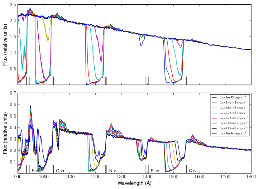
To investigate whether we can increase substantially while retaining the observed BAL features for sightlines looking into the wind cone, Figure 11 shows the behaviour of the emergent spectra for and as the X-ray luminosity is increased from to . We will focus on the behaviour of C iv and O vi as representative examples. For , the C iv BAL feature becomes narrower with increasing : it gradually disappears, starting from the blue edge. The feature is lost entirely by . The effect on the O vi feature is more abrupt, with almost no effect up to a luminosity of , but complete disappearance for twice that luminosity. Similarly, for , C iv weakens gradually in models with larger , while in this case O vi shows hardly any response to until we reach . Note that C iv is still present with a clear BAL signature at this X-ray luminosity for .
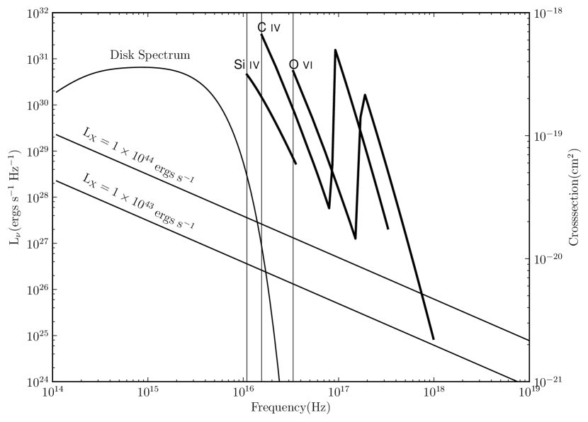
The strong sensitivity of the UV resonance transition to in this range can be understood by considering the location of the photoionization edges for these species. Figure 12 shows these locations relative to the angle-averaged disk spectrum and the X-ray spectra corresponding to and . The ionization edge of C iv falls very close to the frequency above which the X-ray source takes over from the disk as the dominant spectral component. In fact, for , photo-ionization of C iv is driven primarily by disk photons, while for , it is mainly due to photons from the X-ray source. The photo-ionization rate of higher-ionization species like O vi is dominated by the X-ray source even at .
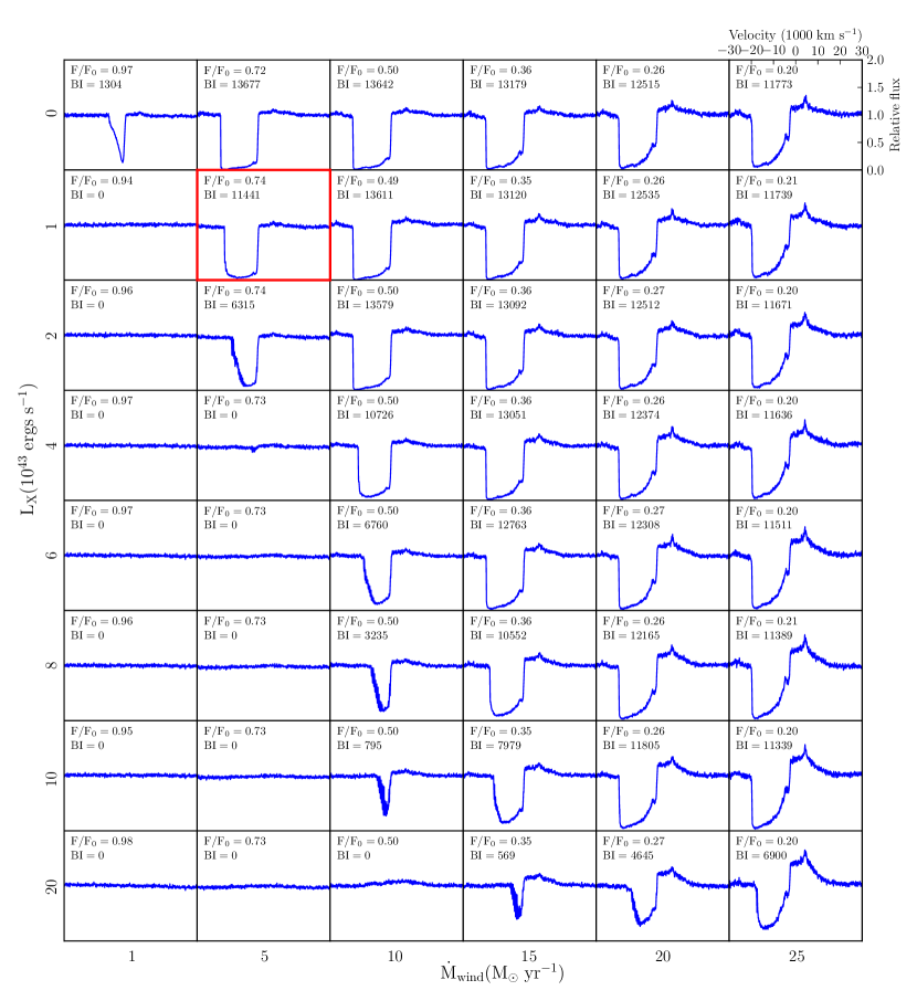
We conclude that moderate increases in (by a factor of a few) would be feasible without any other parameter adjustments, but larger changes will begin to destroy BAL features for more and more sightlines. However, it is reasonable to anticipate that the negative effects of increasing on BAL features may be mitigated by simultaneously increasing the mass-loss rate in the wind, . We have therefore carried out a 2-dimensional sensitivity study, in which we vary both and . The results – focussing particularly on the key C iv line profile for – are shown in Figure 13. In each panel of this figure, we also give the BI measured for the profile shown, as well as values of ; the ratio of the continuum at to that obtained in a model without a wind.
The second column in Figure 13 illustrates the effect of increasing while keeping the mass-loss rate at the benchmark value of (as in Figure 11). We see again that the C iv BAL feature persists up to at least , although it becomes both weaker and narrower with increasing . For higher mass-loss rates (third and beyond columns in Figure 13), the C iv profile becomes increasingly insensitive to . So, as expected, increasing allows for the production of strong BAL features in species like C iv even at higher irradiating . Thus one way to address the X-ray weakness of the benchmark model (i.e. increase ) is to increase both and .
This remedy has a side effect: any increase in also implies an increase in , the electron-scattering optical depth through the outflow. This reduces the observed X-ray and and optical luminosity of the BALQSO. For moderate inclinations and mass-loss rates, the emergent continuum flux will scale simply as , although for the highest inclinations and , scattered radiation will dominate the continuum and break this scaling. In any case, our main conclusion is that, for high mass-loss rates, we are able to produce BALs over a wider range of but at the expense of significant continuum suppression. If this is to provide a realistic route towards geometrical unification, it implies that the intrinsic luminosities of BALQSOs must be higher than suggested by their observed brightness.
There are, of course, other possibilities. For example, if the outflow is clumpy (e.g. Krolik, McKee & Tarter, 1981; Arav et al., 1999), some of the X-ray radiation may pass through the wind unimpeded, thus increasing the observed for sightlines inside the wind cone. Such a solution would have the added advantage that the higher density within the clumps would naturally result in a lower ionization state for a given X-ray flux. Relaxing the assumption of a smooth flow would, of course, take us back in the direction of cloud models of the BLR and BALR. We plan to investigate the pros and cons of such scenarios in future work.
6.2 The Weakness of Line Emission Produced by the Outflow
As mentioned in Section 5.2.2, our benchmark model does not produce strong emission line features, especially at low inclination models where the geometric unification scenario suggests Type I QSOs should be seen. This suggests that modifications are required in some aspect of the structure or the physics that is incorporated into python, if the geometric unification scenario is correct.
In considering this shortcoming, it is interesting to compare with the disk wind modelling carried out by Murray et al. 1995 [hereafter MCGV95]. They explicitly model a line-driven outflow, and the broad characteristics of their disk wind are sufficiently similar to our benchmark model to make a comparison interesting. MCGV find that their outflow produces BAL troughs when viewed at high inclinations. However, they also find that their model produces sufficient collisionally excited emission in species like C iv to explain the BEL in both BALQSOs and non-BAL QSOs. In their model, this C iv emission arises in a layer of the wind close to the disk plane where C iv is the dominant ionization stage of carbon. They argue that this region extends from to and is characterized by and . It is the integrated, collisionally excited emission from this region that dominates the C iv line flux in their model.
In the case of our benchmark model, Figure 5 shows that the fractional C iv abundance is high () in a region extending from to . However, the density in this region is considerably lower than in the C iv line-forming region considered by MCGV: . It is this lower density that almost certainly explains the difference in C iv emissivity in the models. In a later version of their model (Murray & Chiang, 1998), the production of C iv is dominated by lower density () material lying at larger radii . In these models, it is the large emitting volume that explains the strength of collisionally excited C iv feature.
These comparisons suggest that moderate changes to the benchmark model may be enough to produce BELs via collisionally excited line emission in the outflow. It is likely that such changes would go in the direction of increasing the density in some parts of the wind, either by modifying existing wind parameters or by introducing clumpiness. In fact, we can clearly see that the emission component of the C iv line in Figure 13 does increase with increasing . However, even our highest models do not yet produce enough emission at low inclination angles. Thus, while the benchmark model shows some promise in the context of geometric unification, it remains to be seen whether (and how) it can be modified to produce the strong emission lines seen in both BALQSOs and non-BAL QSOs. This will be the subject of a separate paper.
Before we leave this section, it is interesting to ask why the scattering of C iv photons in the outflow does not produce emission lines of sufficient strength in our model. In CV winds, for example, modelling suggests that resonance scattering is the primary mechanism for producing the observed emission line profiles (Shlosman & Vitello 1993; Knigge, Woods & Drew 1995, LK02, Noebauer et al. 2010). The critical factor in understanding the relative importance of scattered photons to the line formation process is the combination of foreshortening, limb-darkening, outflow orientation and covering factor. The outflows in CVs are thought to be ejected roughly perpendicular to the accretion disk, albeit over quite a large range of opening angles. Moreover, CV winds emerge directly above the continuum emitting regions of the disk, whereas BALQSO winds cover only as seen from the continuum source. Thus, in a CV, an outflow that is optically thick in C iv over some velocity interval will intercept virtually all of the continuum photons within this interval – and scatter them into other sightlines, where they emerge as apparent line emission. Conversely, our QSO wind scatters only a small fraction of the continuum photons, even in frequency intervals in which the wind is optically thick. As a result, scattered photons will not contribute as much to emission line formation.
6.3 Ionization Stratification and Reverberation Mapping
In our benchmark model, the ionization state of the outflow tends to increase with increasing distance along poloidal streamlines (Figure 5). This is easily understood. Far away from the central engine, in the region of the flow where the BAL features are produced, the wind geometry approximates an optically thin, spherical outflow. In such an outflow, , so as long as the wind accelerates, the ionization parameter must also increase outwards.
This trend may appear to contradict reverberation mapping studies of the BLR, which suggest ionization stratification in the opposite sense. For example, the C iv BLR radius at fixed UV luminosity inferred by Kaspi et al. (2007) is smaller than that obtained by Kaspi et al. (2005) for H. This sense of ionization stratification is also supported by recent microlensing results (e.g. Guerras et al., 2013).
However, our model is not necessarily in conflict with these empirical findings. As discussed in Section 6.2, it is clear that the parts of the wind producing BALs (where increases outwards) are unlikely to be co-spatial with the parts of the wind producing BELs. More specifically, only the dense base of the disk wind is likely to produce significant amounts of collisionally excited line emission. Thus, in the context of disk wind models, the reverberation mapping results are unlikely to probe the “radial” ionization structure of the outflow, but may instead probe the stratification along the base of the wind in the direction. Here, the ionization parameter can (and does) decrease outwards in our disk wind models.
6.4 Implications
Here we consider implications of our benchmark model for AGN feedback in galaxy evolution and identifying possible driving mechanisms for the wind.
In energetic terms, effective feedback – sufficient to establish the relation, for example – seems to require (Di Matteo et al., 2005; Hopkins & Elvis, 2010). Here, is the kinetic luminosity of the outflow. Our benchmark model is characterized by and , which yields . Thus an outflow of this type would be capable of providing significant amounts of energy-driven feedback. The kinetic luminosity of the benchmark model is also broadly in line with the empirical scaling between and found by King et al. (2013) for black holes across the entire mass-scale, from compact binary systems to AGN/QSO.
King (2003, 2005, 2010) has argued that QSO outflows interact with their host galaxy in a momentum-, rather than energy-driven fashion. In this case, the strength of the feedback an outflow can deliver depends on its momentum flux, . This scenario naturally produces the observed relation if the outflows responsible for feedback satisfy ; this is the single-scattering limit for momentum transfer in a radiatively-driven outflow from a QSO radiating at . For our benchmark model, we find . In other words, the momentum flux in our model is close to the single-scattering limit for its bolometric luminosity. Since black hole growth and cosmological feedback are thought to be dominated by phases in which (Soltan, 1982; Yu & Tremaine, 2002; Di Matteo et al., 2005), outflows of this type would probably also meet momentum-based feedback requirements.
The momentum flux in the outflow is also a key parameter for any disk wind driven by radiation pressure, such as the line-driven winds considered by MCGV95 and Proga, Stone & Kallman (2000). In particular, such winds typically satisfy the single-scattering limit for momentum transfer from the radiation field to the outflow, . As noted above, our benchmark model also satisfies this limit. However, this is somewhat misleading: our disk wind subtends only of the sky as seen from the central source, and it intercepts an even smaller fraction of the QSOs bolometric luminosity (due to foreshortening and limb-darkening of the disk radiation field). The momentum flux in our benchmark model actually exceeds the single-scattering limit if only momentum carried by photons that actually intercept the wind is taken into account. Thus, in the context of radiatively-driven winds, either the mass-loss rate in our model must be overestimated or multiple scattering effects must be important. The latter has been suggested for quasi-spherical Wolf-Rayet star winds (Lucy & Abbott, 1993; Springmann, 1994; Gayley, 1995) but is much more challenging for the biconical wind considered here. Alternatively, the winds of QSOs may not be driven (exclusively) by radiation pressure, with magnetic/centrifugal forces providing the most obvious alternative (e.g. Blandford & Payne, 1982; Emmering et al., 1992; Proga, 2003).
Our discussion of all these considerations is preliminary: the benchmark model is far from perfect, and we have not yet carried out a comprehensive survey of the available parameter space. However, the first column in Figure 13 shows that a reduction in the mass-loss rate from the benchmark value of to virtually destroys the BAL features, even for . Thus, at least for our adopted wind geometry and kinematics, it seems that any outflow capable of producing BAL features is also likely to provide significant feedback and pose a challenge to line-driving.
6.5 Outlook
In our view, the most significant shortcomings of the benchmark model are its intrinsic X-ray weakness and its inability to produce collisionally excited BELs. Both problems might be resolved by moderate changes in wind parameters, so an important step will be to explore the parameter space of our model. We plan to adopt two complementary approaches in this: (i) systematic grid searches; (ii) targeted explorations guided by physical insight. The latter approach is important, since compromises will have to be made in the former: a detailed and exhaustive search over all relevant parameters is likely to be prohibitive in terms of computational resource requirements. As an example of how physical insight can guide us, we note that both the X-ray and emission line problems might be resolved by increasing the density in specific wind regions.
7 Summary
This paper represents the first step in a long-term project to shed light on the nature of accretion disk winds in QSOs. These outflows may be key to the geometric unification of AGN/QSO and might also provide the feedback required by successful galaxy evolution scenarios.
In this pilot study, we have focussed on the most obvious signature of these outflows, the broad, blue-shifted absorption lines seen in of QSOs. We have constructed a kinematic disk wind model to test if it can reproduce these features. This benchmark model describes a rotating, equatorial and biconical accretion disk wind with a mass-loss rate .555 Strictly speaking, this is not entirely self-consistent, since the presence of such an outflow would alter the disk’s temperature structure. However, we neglect this complication, since the vast majority of the disk luminosity arises from well within our assumed wind-launching radius. A Monte Carlo ionization and radiative transfer code, python, was used to calculate the ionization state of the outflow and predict the spectra emerging from it for a variety of viewing angles. Our main results are as follows:
-
(i)
Our benchmark model succeeds in producing BAL-like features for sightlines towards the central source that lie fully within the wind cone.
-
(ii)
Self-consistent treatment of ionization and radiative transfer is necessary to reliably predict the ionization state of the wind and the conditions under which key species like C iv can efficiently form.
-
(iii)
The benchmark model does not produce sufficient collisionally excited line emission to explain the BELs in QSOs. However, we argue that moderate modifications to its parameters might be sufficient to remedy this shortcoming.
-
(iv)
The ionization structure of the model, and its ability to produce BALs, are quite sensitive to the X-ray luminosity of the central source. If this is too high, the wind becomes overionized. In our benchmark model, is arguably lower than indicated by observations. Higher values of may require higher outflow columns – e.g. via higher – in order to still produce BALs.
-
(v)
For our adopted geometry and kinematics, is required in order to produce significant BAL features. The kinetic luminosity and momentum carried by such outflows is sufficient to provide significant feedback.
Acknowledgements
The work of NH, JHM and CK are supported by the Science and Technology Facilities Council (STFC), via studentships and a consolidated grant, respectively. The authors would like to thank the anonymous referee for useful comments.
References
- Abbot & Lucy (1985) Abbot, D. C. & Lucy, L. B. 1985, ApJ, 288, 679A
- Allen et al. (2011) Allen, J. T., Hewett, P. C., Maddox, N., Richards, G. T. & Belokurov, V. 2011, MNRAS, 410, 860
- Arav et al. (1995) Arav, N., Korista, K. T., Barlow, T. A. & Begelman. 1995, Nature, 376, 576
- Arav (1996) Arav, N. 1996, ApJ, 465, 617
- Arav et al. (1999) Arav, N., Korista, K. T., de Kool, M., Junkkarinen, V. T. & Begelman, M. C. 1999, ApJ, 516, 27
- Arav et al. (2008) Arav, N., Moe, M., Costantini, E., Korista, K. T., Benn, C. & Ellison, S., 2008, ApJ, 681, 954
- Badnell (2006) Badnell, N. R. 2006, ApJs, 167, 334
- Becker et al. (2000) Becker, R. H., White, R. L., Gregg, M. D., Brotherton, M. S., Laurent-Muehleisen, S. A. & Arav, N., 2000, ApJ, 538, 72
- Begelman, Blandford & Rees (1984) Begelman, M. C., Blandford, R. D. & Rees, M. J. 1984, Reviews of Modern Physics, 56, 255
- Blandford & Payne (1982) Blandford, R. D. & Payne, D. G. 1982, MNRAS, 199, 883
- Blundell et al. (2001) Blundell, K. M., Mioduszewski, A. J., Muxlow, T. W. B., Podsiadlowski, P. & Rupen, M. P. 2001, ApJl, 562, L79
- Borguet & Hutsemékers (2010) Borguet, B. & Hutsemékers, D. 2010, A&A, 515, A22
- Bottorff et al (1997) Bottorff, M., Korista, K. T., Shlosman, I. & Blandford, R. D. 1997, ApJ, 479, 200
- Brotherton, De Breuck & Schaefer (2006) Brotherton, M. S., De Breuck, C. & Schaefer, J. J. 2006, MNRAS, 372, L58
- Capellupo et al. (2011) Capellupo, D. M., Hamann, F., Shields, J. C., Rodríguez Hidalgo, P. & Barlow, T. A. 2011, MNRAS, 413, 908
- Capellupo et al. (2012) Capellupo, D. M., Hamann, F., Shields, J. C., Rodríguez Hidalgo, P. & Barlow, T. A. 2012, MNRAS, 422, 3249
- Capellupo et al. (2013) Capellupo, D. M., Hamann, F., Shields, J. C., Halpern, J. P. & Barlow, T. A. 2013, MNRAS, 429, 1872
- Cloudy & associates (2011) Hazy, a brief introduction to cloudy C10
- Cordova & Mason (1982) Cordova, F. A. & Mason, K. O. 1982, ApJ, 260, 716
- Cottis et al. (2010) Cottis, C. E., Goad, M. R., Knigge, C. & Scaringi, S. 2010, MNRAS, 406, 2094
- Cunto et al. (1993) Cunto, W., Mendoza, C., Ochsenbein, F. & Zeippen, C, J. 1993, A&A, 275, L5
- Dere et al. (1997) Dere, K. P., Landi, E., Mason, H. E., Monsignori Fossi, B. C. and Young, P. R. 1997, A&As, 125, 149
- Di Matteo et al. (2005) Di Matteo, T., Springel, V. & Hernquist, L. 2005, Nature, 433, 604
- Done et al. (2012) Done, C., Davis, S. W., Jin, C., Blaes, O. & Ward, M. 2012, MNRAS, 420, 1848
- Elvis (2000) Elvis, M. 2000, ApJ, 545, 63
- Emmering et al. (1992) Emmering, R. T., Blandford, R. D. & Shlosman, I. 1992, ApJ, 385, 460
- Everett, Königl & Karje (2001) Everett, J. E., Königl, A. & Kartje, J. F. 2001, ASP Conf. Ser. 224: Probing the Physics of Active Galactic Nuclei, 224, 441
- Everett, Königl & Arav (2002) Everett, J., Königl, A. & Arav, N. 2002, ApJ, 569, 617
- Fabian (2012) Fabian, A. C. 2012, ARA&A, 50, 455
- Fender (2006) Fender, R., 2006, in Compact stellar X-ray sources, ed Lewin, W. H. G. & van der Klis, M. (Cambridge: Cambridge Univ. Press); 381
- Ferland et al. (2013) Ferland, G. J., Porter, R. L., van Hoof, P. A. M., Williams, R. J. R., Abel, N. P., Lykins, M. L., Shaw, G., Henney, W. J. & Stancil, P. C. 2013, Rev. Mexicana Astron. Astrofis., 49, 137
- Galeev, Rosner & Vaiana (1979) Galeev, A. A., Rosner, R. & Vaiana, G. S. 1979, ApJ, 229, 318
- Ganguly at al. (2006) Ganguly, R., Sembach, K. R., Tripp, T. M., Savage, B. D. & Wakker, B. P. 2006, ApJ, 645, 868
- Ganguly & Brotherton (2008) Ganguly, R. & Brotherton, M. S., 2008, ApJ, 672, 102
- Gayley (1995) Gayley, K. G. ApJ, 454, 410
- Gibson et al. (2009) Gibson, R. R., Jiang, L., Brandt, W. N., Hall, P. B., Shen, Y., Wu, J., Anderson, S. F., Schneider, D. P., Vanden Berk, D., Gallagher, S. C., Fan, X. & York, D. G. 2009, ApJ, 692, 758
- Giustini, Cappi & Vignali (2008) Giustini, M., Cappi, M. & Vignali, C. 2008, A&A, 491,425
- Giustini & and Proga (2012) Giustini, M. & Proga, D. 2012, ApJ, 758, 70
- Granato et al. (2001) Granato, G. L., Silva, L., Monaco, P., Panuzzo, P., Salucci, P., De Zotti, G. & Danese, L. 2001, MNRAS, 324,757
- Greenstein & Oke (1982) Greenstein, J. L. & Oke, J. B. 1982, ApJ, 258, 209
- Guerras et al. (2013) Guerras, E., Mediavilla, E., Jimenez-Vicente, J., Kochanek, C. S., Muñoz, J. A., Falco, E. & Motta, V. 2013, ApJ, 764. 160
- Hewett & Foltz (2003) Hewett, P. C., & Foltz, C, B. 2003, AJ, 125, 1784
- Hopkins & Elvis (2010) Hopkins, P. F. & Elvis, M. 2010, MNRAS, 401, 7
- Just et al. (2007) Just, D. W., Brandt, W. N., Shemmer, O., Steffen, A. T., Schneider, D. P., Chartas, G. & Garmire, G. P. 2007, ApJ, 665, 1004
- Kaspi et al. (2005) Kaspi, S., Maoz, D., Netzer, H., Peterson, B. M., Vestergaard, M. & Jannuzi, B. T. 2005, ApJ, 629, 61
- Kaspi et al. (2007) Kaspi, S., Brandt, W. N., Maoz, D., Netzer, H., Schneider, D. P. & Shemmer, O. 2007, ApJ, 659, 997
- Kaspi et al. (2000) Kaspi, S., Smith, P. S., Netzer, H., Maoz, D., Jannuzi, B. T. & Giveon, U. 2000, ApJ, 533, 631
- Kellerman et al. (1989) Kellermann, K. I., Sramek, R., Schmidt, M., Shaffer, D. B. & Green, R. 1989, AJ, 98, 1195
- King (2003) King, A. 2003, ApJl, 596, L27
- King (2005) King, A. 2005, ApJl, 635, L121
- King (2010) King, A. R. 2010, MNRAS, 402, 1516
- King et al. (2013) King, A. L., Miller, J. M., Raymond, J., Fabian, A. C., Reynolds, C. S., Gültekin, K., Cackett, E. M., Allen, S. W., Proga, D., & Kallman, T. R. 2013, ApJ, 762, 103
- Knigge (1999) Knigge, C. 1999, MNRAS, 309, 409
- Knigge, Woods & Drew (1995) Knigge, C., Woods, J. A. & Drew, J. E. 1995, MNRAS, 273, 225
- Knigge et al. (2008) Knigge, C., Scaringi, S., Goad, M. R., & Cottis, C. E. 2008, MNRAS, 386, 1426
- Körding et al. (2011) Körding, E. G., Knigge, C., Tzioumis, T. & Fender, R. 2011, MNRAS, 418, L129
- Krolik, McKee & Tarter (1981) Krolik, J. H., McKee, C. F. & Tarter, C. B. 1981, ApJ, 249, 422
- Krolik & Voit (1998) Krolik, J. H. & Voit, G. M. 1998, ApJ, 497, L5
- Lada (1985) Lada, C. J. 1985, ARA&A, 23, 267
- Landi et al. (2012) Landi, E., Del Zanna, G., Young, P. R., Dere, K. P. & Mason, H. E. 2012, ApJ, 744, 99
- Long & Knigge (2002) Long, K. S. & Knigge, C. 2002 ApJ, 579, 725L
- Lucy (1999) Lucy, L. B. 1999, A&A, 345, 211
- Lucy & Abbott (1993) Lucy, L. B. & Abbott, D. C., ApJ, 405, 738
- Marsh & Horne (1988) Marsh, T. R. & Horne, K. 1988, MNRAS, 235, 269
- McNamara & Nulsen (2007) McNamara, B. R. & Nulsen, P. E. J. 2007, ARA&A, 45, 117
- Morton (1967) Morton, D. C., 1967, ApJ, 150, 535
- Murray et al. (1995) Murray, N., Chiang, J., Grossman, S. A. & Voit, G. M. 1995, ApJ, 451, 498
- Murray & Chiang (1996) Murray, N. & Chiang, J. 1996, Nature, 382, 789
- Murray & Chiang (1998) Murray, N. & Chiang, J. 1998, ApJ, 494, 125
- Neilsen & Lee (2009) Neilsen, J. & Lee, J. C. 2009, Nature, 458, 481
- Noebauer et al. (2010) Noebauer, U. M., Long, K. S., Sim, S. A. & Knigge, C. 2010, ApJ, 719, 1932
- North, Knigge & Goad (2006) North, M., Knigge, C. & Goad, M. 2006, MNRAS, 365, 1057
- Ogle et al. (1999) Ogle, P. M., Cohen, M. H., Miller, J. S., Tran, H. D., Goodrich, R. W., & Martel, A. R. 1999, ApJs, 125, 1
- Ponti et al. (2012) Ponti, G., Fender, R. P., Begelman, M. C., Dunn, R. J. H., Neilsen, J. & Coriat, M. 2012, MNRAS, 422, L11
- Proga (2003) Proga, D. 2003, ApJ, 585, 406
- Proga & Kallman (2004) Proga, D. & Kallman, T. R. 2004, ApJ, 616, 688P
- Proga, Stone & Kallman (2000) Proga, D., Stone, J. M. & Kallman, T. R. 2000, ApJ, 543, 686
- Risaliti & Elvis (2010) Elvis, M. & Risaliti, G. 2010 A&A, 516A, 89R
- Reichard et al. (2003) Reichard, T. A., Richards, G. T., Hall, P. B., Schneider, D. P., Vanden Berk, D. E., Fan, X., York, D. G., Knapp, G. R. & Brinkmann, J. 2003, AJ, 126, 2594
- Schawinski (2007) Schawinski, K., Thomas, D., Sarzi, M., Maraston, C., Kaviraj, S., Joo, S. J., Yi, S. K. & Silk, J. 2007, MNRAS, 382, 1415
- Schurch & Done (2007) Schurch, N. J. and Done, C. 2007, MNRAS, 381, 1413
- Schurch, Done & Proga (2009) Schurch, N. J., and Done, C. & Proga, D. 2009, ApJ, 694, 1
- Shakura & Sunyaev (1973) Shakura, N. I. & Sunyaev, R. A. 1973, A&A, 24, 337
- Shlosman & Vitello (1993) Shlosman, I & Vitello, P. 1993, ApJ, 409, 372S
- Sim (2005) Sim, S. A. 2005, MNRAS, 356, 531
- Sim et al. (2005) Sim, S. A., Drew, J. E. & Long, K. S. 2005, MNRAS, 363, 615
- Sim et al. (2008) Sim, S. A., Long, K. S., Miller, L. & Turner, T. J. 2008, MNRAS, 388, 611S
- Sim et al. (2010) Sim, S. A., Miller, L., Long, K. S. & Turner, T. J. 2010, MNRAS , 404, 1369
- Simon & Hamann (2010) Simon, L. E. & Hamann, F. 2010, MNRAS, 409, 269
- Smak (1981) Smak, J. 1981, Acta Astron. 31, 395
- Soltan (1982) Soltan, A. 1981, MNRAS, 200, 115
- Springmann (1994) Springmann, U. 1994, A&A, 289, 505
- Sutherland (1998) Sutherland, R. S. 1998, MNRAS, 300, 321S
- Treister, Urry & Virani (2009) Treister, E., Urry, C. M. & Virani, S. 2009, ApJ, 696, 110
- Turner & Miller (2009) Turner, T. J. & Miller, L. 2009, A&Ar, 17, 47
- Verner, Barthel & Tytler (1994) Verner, D. A., Barthel, P. D., & Tytler, D. 1994, A&A, 108, 287
- Verner, Ferland, Korista & Yakovlev (1996) Verner, D. A., Ferland, G. J., Korista, K. T. & Yakovlev, D. ,G. 1996, ApJ, 465, 487
- Verner, Verner & Ferland (1996) Verner, D. A., Verner, E. M., & Ferland, G. J. 1996, Atomic Data and Nuclear Data Tables, 64,1
- Weyman et al. (1991) Weyman, R. J., Morris, S. L., Foltz, C. B. & Hewitt, P. C. 1991, ApJ, 373, 23
- Xu et al. (2008) Xu, Y., Bian, W. H., Yuan, Q. R. & Huang, K. L. 2008, MNRAS, 389, 1703
- Yu & Tremaine (2002) Yu, Q. & Tremaine, S. 2002, MNRAS, 335, 965
- Zhou et al. (2006) Zhou, H., Wang, T., Wang, H., Wang, J., Yuan, W.,& Lu, Y. 2006, ApJ, 639, 716