Backreaction of a massless minimally coupled scalar field from inflationary quantum fluctuations

Abstract

In this paper we study a massless, minimally coupled scalar field in a FLRW spacetime with periods of different constant deceleration parameter. We assume the Bunch-Davies vacuum during inflation and then use a sudden matching approximation to match it onto radiation era and subsequently onto matter era. We then proceed to calculate the one-loop energy-momentum tensor from the inflationary quantum vacuum fluctuations in different eras. The energy-momentum tensor has the form of an ideal (quantum) fluid, characterized by an equation of state. When compared with the background, far away from the matching the quantum energy density in radiation era exhibits a contribution that grows logarithmically with the scale factor. In matter era the ratio of the quantum to classical fluid settles eventually to a tiny constant, $\rho_{q}/\rho\simeq(\hbar H_{0})^{2}/(4\pi m_{\rm P}^{2}c^{4})\sim 10^{-13}$ for a grand unified scale inflation. Curiously, the late time scaling of quantum fluctuations suggests that they contribute a little to the dark matter of the Universe, provided that it clusters as cold dark matter, which needs to be checked.

I Introduction and motivation

There has been some excitement concerning the possibility that inflationary vacuum fluctuations can play the role of dark energy today KolbMatarreseRiotto ; BarausseMatarreseRiotto . It was subsequently argued that that was not the case HirataSeljak . That question was never completely settled by performing a proper quantum field theoretic calculation.

Somewhat earlier, in the early 2000s, some progress has been made as regards the (one-loop) backreaction of scalar cosmological perturbations during inflation Abramo:2001dc ; Abramo:2001db ; Abramo:1998hj ; Abramo:1998hi ; Geshnizjani:2002wp ; Geshnizjani:2003cn ; Abramo:2001dd . The question of backreaction is particularly delicate during inflation since the main contribution to the backreaction during this era originates from super-Hubble scales and different observers will disagree regarding how to define the backreaction. A consensus has been reached that a reasonable (local) observer will observe a local expansion rate Geshnizjani:2002wp ; Geshnizjani:2003cn ; Abramo:2001dd , or an expansion rate that contains information collected along the past light cone Abramo:2001dc ; Abramo:2001db ; Abramo:1998hj ; Abramo:1998hi . In both viewpoints the same conclusion was reached: at one-loop cosmological perturbations produce vanishing backreaction. This conclusion was disappointing and has contributed to stopping any further investigation of quantum backreaction, including that on late time observers .

What holds for inflationary observers is not generally true for late time observers. Namely, at late times many of the modes that were super-Hubble during inflation, become sub-Hubble, and they may have an impact on observations. The main purpose of this paper is to study the one-loop quantum backreaction of amplified inflationary fluctuations in late time epochs such as radiation and matter era. For simplicity, we concentrate here on the following, somewhat simplified case: we assume a de Sitter inflation, suddenly matched onto a radiation era, that is subsequently matched onto a matter era. We consider quantum fluctuations of a massless, minimally coupled test scalar field and of the graviton, and calculate the corresponding one-loop energy-momentum tensor, which we use to study quantum backreaction. Furthermore, we assume a global Bunch-Davies vacuum state during inflation, and then evolve it by performing the usual sudden matching onto radiation and matter era.

With some care we point out the difficulties that arise from this procedure. Firstly, strictly speaking the global Bunch-Davies vacuum state we use is a singular state in the infrared (IR), making it thus unphysical. For our purposes this state suffices, since the singular nature of the state is not apparent in the one-loop energy-momentum tensor. But the singular nature of the global Bunch-Davies state can become apparent even in a one-loop energy-momentum tensor. For example, the global Bunch-Davies vacuum in matter era exhibits a logarithmic infrared divergence in the one-loop energy-momentum, and the state has to be changed (‘regularized’) in the infrared. Secondly, we perform a sudden matching in between inflation, radiation and matter eras (see figure 1)

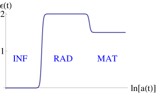
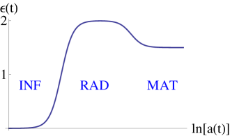
Figure 1: Two possible (realistic) scenarios for the evolution of the slow roll parameter $\epsilon(t)$ in de Sitter inflation, radiation and matter era. Left panel: Sharp transitions, in which the transition time $\tau$ is smaller than the expansion time, $\tau\ll 1/H$. Right panel: Mild transitions, in which $\tau\gtrsim 1/H$.

in the sense that the background geometry exhibits a jump (components of the curvature tensors exhibit a jump). This singular procedure generates extra ultraviolet (UV) divergences, which are manifest in dimensional regularization as an extra divergence $\propto 1/(D-4)$, that scales as radiation, and thus cannot be renormalized by the usual (bulk) counterterms. Furthermore, there are power law boundary divergences that have the same origin, and that are regular at late times. All of these divergences are unphysical, in the sense that they are generated by the unphysical procedure of sudden matching. An example which demonstrates by an exemplary calculation that a smooth transition does not generate any boundary divergences is discussed in Ref. Koivisto:2010pj , but we do not see how that exact solution can be extended to the realistic Universe history we are interested to model in this work. Instead, we introduce an exponential regulator for the Bogolyubov coefficients, which mimics a finite time of transition, thus modeling the physically realistic situation of a smooth transition, and thus demonstrate that all of these boundary divergences are removed. The transition time in the Universe is typically given by the expansion time at that moment. For example, the radiation-matter transition time is of the order of the expansion time at the time of radiation-matter equality. The analogous estimate for the inflation-radiation transition is also reasonable: the time scale of the inflaton decay at the end of inflation (known as (p)reheating) is the expansion time at the end of inflation. However, when non-perturbative effects such as parametric resonance are taken into account, the transition time can become of the order tens of oscillations of the inflaton (dictated by the inflaton mass), which can be much shorter than the expansion time at that time. Hence, since the (p)reheating time is not dictated by the expansion rate, (p)reheating can last much shorter (but also much longer) than the expansion time at the end of inflation, and should be kept as a free parameter (see, for example, Ref. Prokopec:1996rr ).

In this work we calculate the expectation value of the one-loop energy-momentum tensor with respect to a globally defined Bunch-Davies vacuum, and hence any effect that we calculate on the background geometry is of a global character. However, observations are done in our local Universe, and are limited by causality to be within our Hubble volume. The question then arises whether these global effects can have any effect on our local measurements. The answer is affirmative. Namely, a photon moving in a global space-time governed by a global expansion rate $H(t)$ will exhibit a redshift that corresponds to that expansion rate. Of course, on top of this global effect, the photon will also feel the presence of any local fluctuations around $H(t)$. Let us for the sake of argument refer to these local fluctuations as $\delta H(x)$ (a better way of parametrizing this is by making use of the local expansion parameter from the Raychaudhuri equation, see Geshnizjani:2002wp ; Geshnizjani:2003cn ). In this work we do not attempt to estimate the size of these local fluctuations in the expansion rate. However, the procedure of how to estimate their size is clear: one has to calculate the one-loop energy-momentum – energy-momentum correlator, from which one would be able to extract the energy density correlator, $\langle\delta\rho(x)\delta\rho(x^{\prime})/\rho_{0}^{2}(t)\rangle$. This correlator then contains enough information to extract how the Hubble rate fluctuates around the global Hubble rate calculated in this paper. The statement that, on average, photons will exhibit a net change in the expansion rate, and hence a net redshift, stands firm.

The paper is organized as follows. In section II we review the background geometry of a spatially flat universe. This is followed in  III by a brief account of the scalar field quantization on a homogeneous expanding background. The one-loop expression for the scalar energy-momentum tensor is presented in section IV. In section V we present the results for the one-loop energy-momentum tensor in de Sitter, radiation and matter era for a global Bunch-Davies vacuum (some details of this standard calculation are given in Appendix A). Our main results can be found in section VI, where we discuss the one-loop energy-momentum tensor, and the resulting backreaction on the background geometry, in radiation and matter era. A particular attention is devoted to resolving the effects arising from the sudden matching approximation. Finally, in section VII we conclude.

II FLRW background

A spatially flat Friedmann-Lemaître-Robertson-Walker (FLRW) metric, $g_{\mu\nu}$, in $D$ dimensions, written in conformal time, is

$$g_{\mu\nu}(x)=a^{2}(\eta)\eta_{\mu\nu}\,,$$ (1)

where $\eta_{\mu\nu}$ is the Minkowski metric in $D$ dimensions,

$$\eta_{\mu\nu}=\mathrm{diag}(-1,1,1,\dots,1)\,,$$ (2)

$a(\eta)$ is the scale factor describing the time evolution of physical length scales, and conformal time $\eta$ is related to the physical (cosmological) time $t$ via $dt=a(\eta)d\eta$. The reason we are working in conformal time, instead of physical one, is that we find the calculations simpler to perform. We introduce the conformal Hubble rate

$$\mathcal{H}(\eta)=\frac{a^{\prime}(\eta)}{a(\eta)}\,,$$ (3)

which is related to the usual physical Hubble rate by $\mathcal{H}=aH$, $H=\dot{a}/a$, where a prime denotes a differentiation with respect to conformal time, and a dot a differentiation with respect to physical time. The dynamics of this background are described by the Friedmann equations,

$$\left(\frac{\mathcal{H}}{a}\right)^{2}=\frac{8\pi G_{N}}{3c^{2}}\rho+\frac{\Lambda}{3}\ ,$$ (4)

$$\frac{\mathcal{H}^{\prime}-\mathcal{H}^{2}}{a^{2}}=-\frac{4\pi G_{N}}{c^{2}}(\rho+p)\,,$$ (5)

where $\rho$ and $p$ are the energy density and pressure of the background ideal fluid, respectively, $\Lambda$ is the cosmological constant, $G_{N}$ is the Newton’s constant, and $c$ the speed of light. We are not interested in the physical composition of the classical fluid that causes the Universe to expand. We are only concerned with what is its effective equation of state, i.e. how the equation of state parameter $w=p/\rho$ depends on time. Furthermore, we are not interested in fluctuations of the fluid; namely we shall assume that the classical fluid is perfectly homogeneous (that defines the hyper-surface of simultaneity), and that it does not fluctuate. In our toy model, the sole source of (quantum) fluctuations is generated by a massless scalar field. Namely, we shall canonically quantize the field on this fixed background, such that quantum fluctuations of the scalar field are the sole source of density and pressure fluctuations. In addition, we shall present a quantitative argument on how to include the contribution of one-loop (quantum) graviton fluctuations.

From the covariant conservation law,

$$\rho^{\prime}+3{\cal H}(\rho+p)=0\,,$$ (6)

it immediately follows that, in an epoch of constant $w$, the energy density and pressure of a perfect fluid have the following dependence on the scale factor,

$$\rho=\frac{p}{w}=\rho_{0}\left(\frac{a_{0}}{a}\right)^{2\epsilon}\ ,$$ (7)

where $\rho(\eta_{0})=\rho_{0}$, $a(\eta_{0})=a_{0}$, and

$$\epsilon=\frac{3}{2}(1+w)\,$$ (8)

is the so-called slow-roll parameter. A universe whose entire matter content is dominated by one ideal fluid behaves in such a way that its slow-roll parameter is constant,

$$\epsilon\equiv q+1=1-\frac{\mathcal{H}^{\prime}}{\mathcal{H}^{2}}=\mathrm{const}\,,$$ (9)

where $q(t)=-a\ddot{a}/\dot{a}^{2}$ denotes the deceleration parameter. The name of the $\epsilon$ parameter is inherited from the context of inflationary models, but here it does not have to be small. Some important values of this parameter are $\epsilon=2$ for radiation-dominated Universe, $\epsilon=3/2$ for non-relativistic matter-dominated, and $\epsilon=0$ for an inflationary de Sitter universe. For FLRW spacetimes with constant $\epsilon$ parameter the Hubble rate and the scale factor are related as

$$\mathcal{H}=\mathcal{H}_{0}\left(\frac{a_{0}}{a}\right)^{\epsilon-1}\ ,$$ (10)

and the explicit form of the scale factor is

$$a(\eta)=a_{0}\Big{[}1+(\epsilon-1)\mathcal{H}_{0}(\eta-\eta_{0})\Big{]}^{\frac{1}{\epsilon-1}}\,,$$ (11)

where $a(\eta_{0})=a_{0}$, and $\mathcal{H}(\eta_{0})=\mathcal{H}_{0}$. In figure 1 we show two examples of possible evolution of $\epsilon(t)$ throughout the history of the Universe: a period of inflation is followed by a period of radiation and matter era. On the left panel the transitions are quite sharp, i.e. the rate of transition between different epochs is much larger than the expansion of the Universe, while on the right panel the transition rate is quite mild. It is very hard to treat either of the two scenarios analytically, so one has to resort to approximations. In this work we shall assume that transitions are sharp, and discuss in some detail the physical effects generated by a sharp transition.

III Scalar field on FLRW

The action of a massless, minimally coupled real scalar field living on a curved background is given by

$$S_{\phi}=-\frac{1}{2}\int d^{D}x\sqrt{-g}g^{\mu\nu}\partial_{\mu}\phi\partial_{\nu}\phi\ .$$ (12)

Canonical quantization of this field on a FLRW background proceeds by first defining a canonical momentum,

$$\pi(x)=\frac{\delta S_{\phi}}{\delta\phi^{\prime}}=a^{D-2}\phi^{\prime}(x)\ ,$$ (13)

and then promoting the fields into operators, $\phi\rightarrow\hat{\phi}$, $\pi\rightarrow\hat{\pi}$, such that they satisfy the following canonical commutation relations,

$$[\hat{\phi}(\eta,\boldsymbol{x}),\hat{\pi}(\eta,\boldsymbol{x}^{\prime})]=[\hat{\phi}(\eta,\boldsymbol{x}),a^{D-2}\hat{\phi}^{\prime}(\eta,\boldsymbol{x}^{\prime})]=i\delta^{D-1}(\boldsymbol{x}-\boldsymbol{x}^{\prime})\ ,$$ (14)

$$[\hat{\phi}(\eta,\boldsymbol{x}),\hat{\phi}(\eta,\boldsymbol{x}^{\prime})]=0=[\hat{\phi}^{\prime}(\eta,\boldsymbol{x}),\hat{\phi}^{\prime}(\eta,\boldsymbol{x}^{\prime})]\,.$$ (15)

When these commutation relations are used in the Heisenberg equation, one obtains the equation of motion for the field operator

$$\hat{\phi}^{\prime\prime}+(D-2)\mathcal{H}\hat{\phi}^{\prime}-\boldsymbol{\nabla}^{2}\hat{\phi}=0\,.$$ (16)

Assuming a spatially homogeneous state $|\Omega\rangle$, the following decomposition of the field operator (in Heisenberg picture) in Fourier modes is convenient,

$$\hat{\phi}(\eta,\boldsymbol{x})=a^{\frac{2-D}{2}}\int\frac{d^{D-1}k}{(2\pi)^{D-1}}\Big{(}{\rm e}^{i\boldsymbol{k}\cdot\boldsymbol{x}}u(k,\eta)\hat{a}(\boldsymbol{k})+{\rm e}^{-i\boldsymbol{k}\cdot\boldsymbol{x}}u^{*}(k,\eta)\hat{a}^{{\dagger}}(\boldsymbol{k})\Big{)}\,,$$ (17)

where the assumed spatial homogeneity of the state dictates that the mode functions $u(k,\eta)$ and $u^{*}(k,\eta)$ depend on the modulus $k=\|\boldsymbol{k}\,\|$ only. The annihilation operator, $\hat{a}$, and the creation operator, $\hat{a}^{{\dagger}}$, satisfy

$$[\hat{a}(\boldsymbol{k}),\hat{a}^{{\dagger}}(\boldsymbol{k}^{\prime})]=(2\pi)^{D-1}\delta^{D-1}(\boldsymbol{k}-\boldsymbol{k}^{\prime})\,,\ \ \ [\hat{a}(\boldsymbol{k}),\hat{a}(\boldsymbol{k}^{\prime})]=[\hat{a}^{\dagger}(\boldsymbol{k}),\hat{a}^{{\dagger}}(\boldsymbol{k}^{\prime})]=0\,,$$ (18)

which fixes the Wronskian normalization of the mode functions,

$$W[u(k,\eta),u^{*}(k,\eta)]=u(k,\eta)\,u^{\prime*}(k,\eta)-u^{*}(k,\eta)\,u^{\prime}(k,\eta)=i\ .$$ (19)

The equation of motion for these mode functions is

$$u^{\prime\prime}(k,\eta)+\left[k^{2}+f(\eta)\right]u(k,\eta)=0\ ,$$ (20)

where $f$ is a time dependent ‘mass term’,

$$f(\eta)=-\frac{D-2}{4}\Big{(}2\mathcal{H}^{\prime}+(D-2)\mathcal{H}^{2}\Big{)}\ .$$ (21)

The name of the creation and annihilation operator is justified by requiring that they construct the Fock space of states. In particular, the vacuum state $|\Omega\rangle$ is defined by

$$\hat{a}(\boldsymbol{k})|\Omega\rangle=0\,,\ \ \ \ (\forall\boldsymbol{k})\,,$$ (22)

and all other states are built by acting on the vacuum state with creation operators. Notice that here we work in Heisenberg picture, in which time evolution is fully contained in the field operator, see Eqs. (16) and (20).

The physical choice of the mode function (the choice of the vacuum) is not as straightforward on curved backgrounds, as it is in Minkowski space, where Poincaré symmetry can be used to uniquely fix the vacuum state. Here we concern ourselves only with this choice on constant $\epsilon$ FLRW backgrounds. The usual choice on accelerating expanding backgrounds ($\epsilon<1$) is the Bunch-Davies vacuum. It is defined by requiring that in the far past ($\eta\rightarrow-\infty$) the modes behave as the positive-frequency conformal Minkowski space mode functions,

$$u(k,\eta)\;\;\stackrel{{\scriptstyle\eta\rightarrow-\infty}}{{\sim}}\;\;\frac{1}{\sqrt{2k}}\,{\rm e}^{-ik\eta}\ ,$$ (23)

Physically, this can be viewed as the requirement that the UV modes behave as those in conformally flat space, which exhibits the Poincaré symmetry of Minkowski space, since all the modes are more and more UV as one goes further to the past. Moreover, one can show that in this adiabatic vacuum the energy density functional, $E[\phi]/V=\int[d^{3}k/(2\pi)^{3}]\varepsilon(k,\eta)$ is minimized. To show that, let us for the moment assume that there is a mode mixing in the asymptotically distant past, such that instead of (23) we have,

$$u(k,\eta)\;\;\stackrel{{\scriptstyle\eta\rightarrow-\infty}}{{\sim}}\;\;\frac{\alpha(k)}{\sqrt{2k}}\,{\rm e}^{-ik\eta}+\frac{\beta(k)}{\sqrt{2k}}\,{\rm e}^{ik\eta}\,,\qquad(|\alpha|^{2}-|\beta|^{2}=1)\,.$$ (24)

It is then easily shown that the corresponding phase-space energy density

$$\varepsilon(k,\eta)\simeq\frac{k}{2}\left(|\alpha|^{2}+|\beta|^{2}\right)\,,$$ (25)

which is clearly minimized for $\beta=0$, giving a very strong argument in favor of the Bunch-Davies vacuum in the UV. The situation can, however, be very different for infrared modes in curved space-times such as expanding FLRW backgrounds, where adiabaticity assumed in deriving (25) is generally broken.

The above definition of the usual Bunch-Davies state relies on the existence of an asymptotic past, which is the case in accelerating universes with $\epsilon<1$. Indeed, in this case asymptotic past means more and more UV when compared to the curvature invariants. In decelerating universes (where $\epsilon>1$) however, asymptotic past does not exist since a decelerating universe starts at a finite time from a curvature singularity (big bang). A simple fix of that problem is to consider the Bunch-Davies vacuum to be the UV state for which the mode functions are (23) when $k/a\gg H$, i.e. physical momenta are large when compared to the space-time curvature, and this is what we shall assume here. One more problem remains, and that is that the above procedure does not say anything about how to pick the state in the IR.

To address that question, in this paper we extend the definition of the Bunch-Davies vacuum, to a global Bunch-Davies vacuum which we define as the analytic extension of the state (23). Namely, while in the UV the distinction between positive and negative frequency modes is straightforward, it is not so in the IR. This analytic extension can be obtained either by analytically extending the asymptotic expansion for the mode functions that satisfy (20) (which can be achieved for example by a Borel resummation), or by simply solving the equation of motion (20) and choosing the solution such that it reduces to (23) in the UV. Both methods will give the unique answer for the global Bunch-Davies vacuum state. When calculating the expectation values of our operators below we shall always perform it with respect to the global Bunch-Davies (BD) vacuum state.

IV Energy-momentum tensor

The energy-momentum tensor operator of a massless, minimally coupled scalar field on a curved background is given by

$$\hat{T}_{\mu\nu}(x)=\left.\frac{-2}{\sqrt{-g}}\frac{\delta S_{\phi}}{\delta g^{\mu\nu}(x)}\right|_{\phi=\hat{\phi}}=\partial_{\mu}\hat{\phi}\,\partial_{\nu}\hat{\phi}-\frac{1}{2}g_{\mu\nu}g^{\alpha\beta}\partial_{\alpha}\hat{\phi}\,\partial_{\beta}\hat{\phi}\ .$$ (26)

Its expectation value on FLRW background, with respect to the global BD vacuum state $|\Omega\rangle$, which is diagonal, can be written in terms of integrals over the mode functions,

$$\langle\Omega|\hat{T}_{00}|\Omega\rangle =\frac{a^{2-D}}{(4\pi)^{\frac{D-1}{2}}\Gamma\left(\frac{D-1}{2}\right)}\int_{0}^{\infty}dk\,k^{D-2}\Bigg{\{}|u^{\prime}|^{2}+\left[k^{2}+\frac{(D-2)^{2}}{4}\mathcal{H}^{2}\right]|u|^{2}-\frac{D-2}{2}\frac{\partial}{\partial\eta}|u|^{2}\Bigg{\}}\ ,$$ (27)

$$\langle\Omega|\hat{T}_{ij}|\Omega\rangle =\frac{\delta_{ij}a^{2-D}}{(4\pi)^{\frac{D-1}{2}}\Gamma\left(\frac{D-1}{2}\right)}$$ (28)

$$\times\int_{0}^{\infty}dk\,k^{D-2}\Bigg{\{}|u^{\prime}|^{2}+\left[-\frac{D-3}{D-1}k^{2}+\frac{(D-2)^{2}}{4}\mathcal{H}^{2}\right]|u|^{2}-\frac{D-2}{2}\mathcal{H}\frac{\partial}{\partial\eta}|u|^{2}\Bigg{\}}\ .$$

The two integrals above, by themselves, generally exhibit quartic, quadratic, and logarithmic UV divergencies in $D=4$. Therefore, these integrals first need to be regularized in the UV, and the method we choose is dimensional regularization, which automatically subtracts power-law divergences. The remaining logarithmic divergence needs to be absorbed into the higher derivative countertems which entails renormalization. The whole procedure of regularization and renormalization of the energy-momentum tensor on FLRW background is presented in Appendix A. In the end one associates finite values to the integrals above, $T_{00}^{q}$ and $T_{ij}^{q}$, which represent the physical expectation values of the energy momentum tensor of the scalar field at one-loop.

It is convenient to express the results in terms of energy density, $\rho_{q}$, and pressure, $p_{q}$,

$$\rho_{q}=\frac{1}{a^{2}}T^{q}_{00}\ ,\ \ \ \delta_{ij}p_{q}=\frac{1}{a^{2}}T_{ij}^{q}\ ,$$ (29)

which can readily be compared to the corresponding values of the classical fluids dictating the dynamics of FLRW background.

V Energy-momentum tensor on FLRW with constant $\epsilon$

In this section we examine the energy-momentum tensor of the scalar field in a Bunch-Davies vacuum on three FLRW backgrounds of constant $\epsilon$ parameter, inflationary one with $\epsilon_{I}=-(D-4)/2$, radiation-dominated one with $\epsilon_{R}={D}/{2}$, and matter-dominated one with $\epsilon_{M}=({D+2})/{4}$. Note that $D$-dependent $\epsilon$ parameters are just our prescription of how to extend their values in $D$=4 to general $D$-dimensional FLRW backgrounds (which are needed in order to employ dimensional regularization). This prescription of extension to $D$ dimensions is essentially arbitrary, and does not influence physical results in $D=4$. The motivation for this prescription is the that it keeps the mode function of the scalar field as simple in $D$ dimensions, as it was in $D$=4. One can see that from the equation of motion (20) on constant $\epsilon$ background, written in terms of the variable $y={k}/[{(1-\epsilon)\mathcal{H}}]$,

$$\left[\frac{d^{2}}{dy^{2}}+1+\frac{\frac{1}{4}-\nu^{2}}{y^{2}}\right]u=0\ ,$$ (30)

where

$$\nu^{2}=\frac{1}{4}+\frac{(D\!-\!2)(D\!-\!2\epsilon)}{4(1\!-\!\epsilon)^{2}}=\left(\frac{D\!-\!1\!-\!\epsilon}{2(1\!-\!\epsilon)}\right)^{2}\ .$$ (31)

The properly normalized positive frequency solution of this equation is

$$u(k,\eta)=\sqrt{\frac{\pi}{4(1-\epsilon)\mathcal{H}}}\,H_{\nu}^{(1)}\left(\frac{k}{(1-\epsilon)\mathcal{H}}\right)\ ,$$ (32)

where $H_{\nu}^{(1)}$ is the Hankel function of the first kind. By requiring (33) we make the order of the Hankel function the same in arbitrary $D$ dimensions as in $D$=4. This is a matter of convenience, proving to be most practical in cases when $\nu=(2n+1)/2$, $n\in\mathbb{N}$ in $D=4$, in which case the Hankel function is just a finite sum. This is the case with all the mode functions we are working with in this paper. This important simplification of mode functions is achieved by promoting $\epsilon$ to a $D$-dependent function $\epsilon_{D}$ according to the prescription

$$\frac{(D-2)(D-2\epsilon_{D})}{(1-\epsilon_{D})^{2}}=\frac{4(2-\epsilon_{4})}{(1-\epsilon_{4})^{2}}\,.$$ (33)

A brief comment regarding dimensional regularization is now warranted, when working with a $D$-dependent $\epsilon$ parameter. Although this prescriptioni will change the finite terms in the UV one obtains from taking the expectation value of the energy-momentum tensor operator, it will also change the finite terms contributed from the counterterm which is to absorb the logarithmic divergence of the energy-momentum tensor. This will happen in such a way that these extra terms exactly cancel when the two are added together. A more explicit elaboration of this statement can be found at the end of Appendix A. As stated above, making $\epsilon$ $D$-dependent does not change the physical result.

V.1 Inflation

On an inflationary background with

$$\epsilon_{I}=-\frac{D-4}{2}\xrightarrow{D\rightarrow 4}0\ ,$$ (34)

the global Bunch-Davies mode functions are

$$u_{I}(k,\eta)=\frac{1}{\sqrt{2k}}\left[1+\frac{i(1\!-\!\epsilon_{I})\mathcal{H}}{k}\right]\exp\left[\frac{ik}{(1\!-\!\epsilon_{I})\mathcal{H}}\right]=\frac{1}{\sqrt{2k}}\left[1+\frac{i(D\!-\!2)\mathcal{H}}{2k}\right]\exp\left[\frac{2ik}{(D\!-\!2)\mathcal{H}}\right]\ .$$ (35)

Even though strictly speaking this mode function defines an IR singular state on de Sitter, for the purposes of this paper this is irrelevant since the one-loop energy-momentum tensor we discuss here is insensitive to the IR singular nature of the state as it is completely regular in the IR. Calculating the one-loop energy-momentum tensor amounts to going through the procedure outlined in Appendix A. The final result is

$$\rho_{q}=-\frac{119\mathcal{H}^{4}}{960\pi^{2}a^{4}}\ ,\ \ \ p_{q}=\frac{119\mathcal{H}^{4}}{960\pi^{2}a^{4}}\ ,$$ (36)

from which we can infer the equation of state parameter,

$$w_{q}=-1=w\ .$$ (37)

From these results it follows that the scalar one-loop fluctuations on de Sitter give a tiny contribution to the cosmological constant,

$$\frac{\delta\Lambda}{\Lambda}=-\frac{119}{360\pi}\bigg{(}\frac{\hbar H}{m_{\rm P}c^{2}}\bigg{)}^{2}$$ (38)

where in the last step we explicitly introduced the dependences on $c$ and $\hbar$, and we defined the usual Planck mass, $m_{\rm P}=\sqrt{\hbar c/G_{N}}$. Although one should add this contribution to the cosmological term, on an exactly de Sitter background it is impossible to disentangle the quantum contribution $\delta\Lambda$ from the classical contribution $\Lambda$.

V.2 Radiation

On a radiation dominated FLRW background with

$$\epsilon_{R}=\frac{D}{2}\xrightarrow{D\rightarrow 4}2\ ,$$ (39)

the global Bunch-Davies mode function is

$$u_{R}(k,\eta)=\frac{1}{\sqrt{2k}}\exp\left[\frac{ik}{(1-\epsilon_{R})\mathcal{H}}\right]=\frac{1}{\sqrt{2k}}\exp\left[-\frac{2ik}{(D-2)\mathcal{H}}\right]\ .$$ (40)

The energy density and pressure associated with this state are

$$\rho_{q}=\frac{\mathcal{H}^{4}}{960\pi^{2}a^{4}}\ ,\ \ \ p_{q}=\frac{\mathcal{H}^{4}}{576\pi^{2}a^{4}}\ ,$$ (41)

and the equation of state parameter is constant,

$$w_{q}=\frac{5}{3}>w=\frac{1}{3}\ ,$$ (42)

which implies the scaling, $\rho_{q}\propto p_{q}\propto 1/a^{8}$. We see that the contribution from the scalar fluctuations decays much faster with the scale factor than the classical fluid driving the expansion, making them negligible at late times.

V.3 Matter

On a non-relativistic matter dominated FLRW background with

$$\epsilon_{M}=\frac{D+2}{4}\xrightarrow{D\rightarrow 4}\frac{3}{2}\ ,$$ (43)

the global Bunch-Davies mode function is

$$u_{M}(k,\eta)=\frac{1}{\sqrt{2k}}\left[1+\frac{i(1\!-\!\epsilon_{M})\mathcal{H}}{k}\right]\exp\left[\frac{ik}{(1\!-\!\epsilon_{M})\mathcal{H}}\right]=\frac{1}{\sqrt{2k}}\left[1\!-\!\frac{i(D\!-\!2)\mathcal{H}}{4k}\right]\exp\left[\frac{-4ik}{(D\!-\!2)\mathcal{H}}\right]\ .$$ (44)

It turns out that on this background the global Bunch-Davies mode functions are not a good physical choice of vacuum in the IR, since it gives rise to an IR divergent one-loop energy-momentum tensor. One has to regularize this IR divergence in some way. Arguably the simplest way is to introduce an IR cut-off $k_{0}$ in the integral defining the energy-momentum tensor, effectively regularizing the IR modes. This regularization can be achieved by placing the Universe in a box of a comoving size $\sim 2\pi/k_{0}$; the discrete mode sums obtained in this way can be replaced by integrals plus corrections suppressed as powers of the IR cut-off scale $k_{0}$. The resulting one-loop energy density and pressure are then

$$\rho_{q}=\frac{9\mathcal{H}^{4}}{128\pi^{2}a^{4}}\left[\ln\left(\frac{\mu_{f}}{k_{0}}a\right)+\frac{61}{270}\right]\ ,$$ (45)

$$p_{q}=\frac{9\mathcal{H}^{4}}{128\pi^{2}a^{4}}\left[\ln\left(\frac{\mu_{f}}{k_{0}}a\right)-\frac{29}{270}\right]\ ,$$ (46)

where $\mu_{f}$ is a free constant that can in principle be determined by measurements. The equation of state parameter is not constant,

$$w_{q}=\frac{\ln\left(\frac{\mu_{f}}{k_{0}}a\right)-\frac{29}{270}}{\ln\left(\frac{\mu_{f}}{k_{0}}a\right)+\frac{61}{270}}\ .$$ (47)

If a proper care is taken to define the initial condition, then $w_{q}>0=w$, meaning that that quantum contribution is negligible. The drawback of this regularization is that it is not valid for all times, since the Hubble rate is a time-evolving scale. At the point when $k_{0}=\mathcal{H}(\eta)$ the regularization breaks down because the cut-off becomes UV instead of IR. Nevertheless, the above expressions for the energy density and pressure are valid for a limited time period. A more proper way to define the vacuum on this background would be to temper the IR behavior of the mode functions by introducing appropriate Bogolyubov coefficients, see e.g. Janssen:2009nz ; Janssen:2008dw .

VI Energy-momentum on FLRW with evolving $\epsilon$

From the three examples of the preceding section we see that, since $w_{q}\geq w$, the global Bunch-Davies state on a period of constant $\epsilon$ does not lead to any significant backreaction. But we know that the time evolution of $\epsilon$ parameter such as illustrated on figure 1 leads to the quantum state evolving away from the Bunch-Davies vacuum state of the particular era, which is often characterized as particle production. That also leads to the different contributions to the energy density and pressure. We study these contributions in this section.

The transitions between different periods of the expansion of the Universe proceed in a smooth manner. These transitions can be described by a time-evolving $\epsilon(\eta)$, which can in principle be determined from the known classical matter content (in the form of perfect fluids) driving the expansion and their interactions. The practical problem is that there are very few $\epsilon(\eta)$ for which the equation of motion for the mode function (20) admits analytically tractable solutions. For an example where such an interpolating solution can be constructed see Ref. Koivisto:2010pj . Even if one can find a solution for the mode function, there is still the task of performing all the integrations in (27–28) to get the energy-momentum tensor. Unless one wants to study the contribution of the quantum fluctuations numerically, approximating the full behavior of $\epsilon(\eta)$ is a necessity.

It is well known that in the case of constant $\epsilon$ one can perform all calculations in the closed form. For this reason we model our FLRW background to have constant $\epsilon$ parameters during some time intervals, and the transitions between different eras are assumed to be instantaneous. By assuming this for the background, we limit the regions where physical predictions for energy density and pressure of the quantum fluctuations can be made. Namely, we do not expect to describe well enough the behavior close to the point of transition, but might be able to determine correctly the late time behavior, if the details of the transition get lost with time. The main purpose of this section is to discuss in some detail how one can make accurate estimates of the one-loop energy momentum tensor at times sufficiently long after the transition.

VI.1 One sudden transition

First, we will address the issues arising from the scale factor of a FLRW background having a discontinuity in its $n$th derivative, $n\geq 2$, at some $\eta_{0}$ (sudden transitions in $\epsilon$ parameter described above correspond to $a^{\prime\prime}(\eta)$ having a discontinuity at $\eta_{0}$). The discontinuity in the background spoils adiabaticity of the mode function in the UV (for momenta $k>\mu\gg\mathcal{H}$), on which we relied in Appendix A to determine the UV divergent structure of $\langle T_{\mu\nu}\rangle$. This discontinuity will induce a mixing of positive and negative frequency modes in the UV, which will not be adiabatically suppressed. Here we derive what this mixing is, how it depends on the order of continuity (or smoothness) of the background, and its influence on the UV part of the energy-momentum tensor.

For $\eta<\eta_{0}$ we assume that the full mode function, $U(k,\eta)$, in the UV is the positive-frequency global Bunch-Davies one, $u(k,\eta)$, given by (102) in Appendix A. A discontinuity in the background at $\eta_{0}$ will spoil adiabaticity of the mode function. The full mode function will still evolve adiabatically after $\eta_{0}$, but it will no longer be a pure positive-frequency function, as the discontinuity in the background will induce some mode mixing. The order of this mixing will depend on the order of discontinuity. After $\eta_{0}$, the full mode function will be a linear superposition of the positive and negative frequency modes,

$$U(k,\eta)=\alpha(k)u(k,\eta)+\beta(k)u^{*}(k,\eta)\ ,$$ (48)

where $u(k,\eta)$ is the UV positive frequency function (102) on a smooth FLRW background for $\eta>\eta_{0}$, and $\alpha(k)$ and $\beta(k)$ are the Bogolyubov coefficients representing mode mixing, which have to satisfy

$$|\alpha(k)|^{2}-|\beta(k)|^{2}=1\ ,$$ (49)

because of the Wronskian normalization (19) being dictated by canonical quantization. These coefficients are the solution of the continuity conditions on the mode function

$$U(k,\eta_{0}^{-})=U(k,\eta_{0}^{+})\ ,\ \ \ U^{\prime}(k,\eta_{0}^{-})=U^{\prime}(k,\eta_{0}^{+})\ ,$$ (50)

where the superscripts on the time arguments signify from which direction the limit to $\eta_{0}$ is taken, $\eta^{\pm}_{0}={\rm lim}_{\delta_{\eta}\rightarrow 0}[\eta_{0}\pm\delta_{\eta}]$. From here, using (102) and (110)-(113), it is straightforward to derive the expressions for $\beta(k)$ in the UV,

$$\beta(k)=e^{-2ik\eta_{0}}\left[\frac{B_{2}}{k^{2}}+\frac{iB_{3}}{k^{3}}+\frac{B_{4}}{k^{4}}+\frac{iB_{5}}{k^{5}}\right]+\mathcal{O}(k^{-6})\ ,$$ (51)

where

$$B_{2}={} \frac{1}{4}\Big{[}f(\eta_{0}^{+})-f(\eta_{0}^{-})\Big{]}\ ,$$ (52)

$$B_{3}={} -\frac{1}{8}\Big{[}f^{\prime}(\eta_{0}^{+})-f^{\prime}(\eta_{0}^{-})\Big{]}\ ,$$ (53)

$$B_{4}={} -\frac{1}{16}\Big{[}f^{\prime\prime}(\eta_{0}^{+})-f^{\prime\prime}(\eta_{0}^{-})+2\Big{(}f^{2}(\eta_{0}^{+})-f^{2}(\eta_{0}^{-})\Big{)}\Big{]}\ ,$$ (54)

$$B_{5}={} \frac{1}{32}\Big{[}f^{\prime\prime\prime}(\eta_{0}^{+})-f^{\prime\prime\prime}(\eta_{0}^{-})+5\Big{(}f^{\prime}(\eta_{0}^{+})f(\eta_{0}^{+})-f^{\prime}(\eta_{0}^{-})f(\eta_{0}^{-})\Big{)}+$$

$$+f^{\prime}(\eta_{0}^{+})f(\eta_{0}^{-})-f^{\prime}(\eta_{0}^{-})f(\eta_{0}^{+})\Big{]}\ ,$$ (55)

and $f(\eta)$ is defined in (21). Calculating $\alpha(k)$ is also straightforward, but for our purposes it suffices to notice that its leading order in UV is always 1, and that it can be written as

$$\alpha(k)=1+\frac{iA_{1}}{k}+\frac{A_{2}}{k^{2}}+\mathcal{O}(k^{-3})\ ,$$ (56)

where $A_{n}$ are real coefficients whose exact value is not important for the present discussion. From (51) and (52)-(55) it is clear how the order of smoothness of the sudden transition relates to the leading order of the Bogolyubov coefficient $\beta$ in the UV, since $f(\eta)$ contains the second time derivative of the scale factor. If the FLRW background has a discontinuity in the $n$th derivative of its scale factor, then the leading order in $\beta(k)$ in the UV will be ${\cal O}(k^{-n})$.

Noting that the squares of the full mode function to be integrated over can be written as

$$|U|^{2} =|u|^{2}+2|\beta|^{2}|u|^{2}+\alpha\beta^{*}u^{2}+\alpha^{*}\beta u^{*2}\ ,$$ (57)

$$|U^{\prime}|^{2} =|u^{\prime}|^{2}+2|\beta|^{2}|u^{\prime}|^{2}+\alpha\beta^{*}u^{\prime 2}+\alpha^{*}\beta u^{\prime*2}\ ,$$ (58)

$$\frac{\partial}{\partial\eta}|U|^{2} =\frac{\partial}{\partial\eta}|u|^{2}+2|\beta|^{2}\frac{\partial}{\partial\eta}|u|^{2}+\alpha\beta^{*}\frac{\partial}{\partial\eta}u^{2}+\alpha^{*}\beta\frac{\partial}{\partial\eta}u^{*2}\ ,$$ (59)

where we used (49), we can split the UV part of the energy-momentum tensor into three parts,

$$\langle\Omega|\hat{T}_{\mu\nu}|\Omega\rangle_{UV}=\langle T_{\mu\nu}\rangle_{UV}^{BD}+\langle T_{\mu\nu}\rangle_{UV}^{\beta}+\langle T_{\mu\nu}\rangle_{UV}^{\alpha\beta}\ ,$$ (60)

to be defined below. The first part, $\langle T_{\mu\nu}\rangle_{UV}^{BD}$, is the part that one also has for a pure positive-frequency Bunch-Davies mode function, as described in Appendix A. We do not need to calculate this contribution again, the results carry over completely. The remaining two terms are a consequence of the mode mixing induced by the background discontinuity. These terms would be zero in the UV if the background was completely smooth. Therefore, we have to examine them more closely.

The middle term in (60) is

$$\langle T_{00}\rangle_{UV}^{\beta}={} \frac{2a^{2-D}}{(4\pi)^{\frac{D-1}{2}}\Gamma\left(\frac{D-1}{2}\right)}\int_{\mu}^{\infty}dk\,k^{D-2}|\beta(k)|^{2}\left\{|u|^{2}+\left[k^{2}+\frac{(D-2)^{2}}{4}\mathcal{H}^{2}\right]|u|^{2}-\mathcal{H}\frac{\partial}{\partial\eta}\right\}$$

$$={} \frac{2a^{2-D}B_{2}^{2}}{(4\pi)^{\frac{D-1}{2}}\Gamma\left(\frac{D-1}{2}\right)}\int_{\mu}^{\infty}dk\,k^{D-5}+\mathcal{O}(\mu^{-2})\ ,$$ (61)

$$\langle T_{ij}\rangle_{UV}^{\beta}={} \frac{2\delta_{ij}a^{2-D}}{(4\pi)^{\frac{D-1}{2}}\Gamma\left(\frac{D-1}{2}\right)}\int_{\mu}^{\infty}dk\,k^{D-2}|\beta(k)|^{2}\left\{|u|^{2}+\left[-\frac{D-3}{D-1}k^{2}+\frac{(D-2)^{2}}{4}\mathcal{H}^{2}\right]|u|^{2}-\mathcal{H}\frac{\partial}{\partial\eta}\right\}$$

$$={} \frac{2a^{2-D}B_{2}^{2}}{(D-1)(4\pi)^{\frac{D-1}{2}}\Gamma\left(\frac{D-1}{2}\right)}\int_{\mu}^{\infty}dk\,k^{D-5}+\mathcal{O}(\mu^{-2})\ ,$$ (62)

where we dropped the $F_{i}$ contributions defined in (102), which is allowed in the UV because $|\beta|^{2}\propto k^{-4}$. The integrals (61–62) are obviously divergent for all times after the matching, provided $B_{2}\neq 0$. The last term in (60) can be immediately evaluated in $D=4$,

$$\langle T_{00}\rangle_{UV}^{\alpha\beta}={} \frac{1}{4\pi^{2}a^{2}}\int_{\mu}^{\infty}dk\,k^{2}\alpha(k)\beta^{*}(k)\left[u^{\prime 2}+\left(k^{2}+\mathcal{H}^{2}\right)u^{2}-\mathcal{H}\frac{\partial}{\partial\eta}u^{2}\right]+{\rm c.c.}$$

$$={} \frac{1}{4\pi^{2}a^{2}}\Big{\{}2B_{2}\mathcal{I}_{0}^{\mu}+\Big{[}B_{2}(\mathcal{H}^{2}-4F_{1}\mathcal{H}+2F_{1}^{\prime}-2A_{1}\mathcal{H})-2B_{3}\mathcal{H}\Big{]}\mathcal{I}_{1}^{\mu}\Big{\}}+\mathcal{O}(\mu^{-1})\ ,$$ (63)

$$\langle T_{ij}\rangle_{UV}^{\alpha\beta}={} \frac{\delta_{ij}}{4\pi^{2}a^{2}}\int_{\mu}^{\infty}dk\,k^{2}\alpha(k)\beta^{*}(k)\left[u^{\prime 2}+\left(-\frac{2k^{2}}{3}+\mathcal{H}^{2}\right)u^{2}-\mathcal{H}\frac{\partial}{\partial\eta}u^{2}\right]+{\rm c.c.}$$

$$={} \frac{\delta_{ij}}{4\pi^{2}a^{2}}\bigg{\{}-\frac{5}{3}B_{2}{\cal I}_{-1}^{\mu}+\bigg{[}B_{2}\Big{(}2{\cal H}-\frac{10}{3}F_{1}-\frac{5}{3}A_{1}\Big{)}-\frac{5}{3}B_{3}\bigg{]}{\cal I}_{0}^{\mu}$$

$$+\bigg{[}B_{2}\Big{(}-\frac{10}{3}F_{2}+2F_{1}^{\prime}+\frac{5}{3}F_{1}^{2}-4{\cal H}F_{1}+{\cal H}^{2}-\frac{5}{3}A_{2}+\frac{10}{3}A_{1}F_{1}-2{\cal H}A_{1}\Big{)}$$

$$+B_{3}\Big{(}-2{\cal H}+\frac{10}{3}F_{1}+\frac{5}{3}A_{1}\Big{)}-\frac{5}{3}B_{4}\bigg{]}{\cal I}_{1}^{\mu}\bigg{\}}+\mathcal{O}(\mu^{-1})\ ,$$ (64)

where the integrals are

$$\mathcal{I}_{-1}^{\mu}={} \int_{\mu}^{\infty}dk\,k\cos(k\Delta)=-\frac{1}{\Delta^{2}}\Big{[}\cos(\mu\Delta)+\mu\Delta\sin(\mu\Delta)\Big{]}\ ,$$ (65)

$$\mathcal{I}_{0}^{\mu}={} \int_{\mu}^{\infty}dk\sin(k\Delta)=\frac{\cos(\mu\Delta)}{\Delta}\ ,$$ (66)

$$\mathcal{I}_{1}^{\mu}={} \int_{\mu}^{\infty}\frac{dk}{k}\cos(k\Delta)=-\mathrm{Ci}(\mu\Delta)\ ,$$ (67)

where $\Delta=2(\eta-\eta_{0})$, and $\mathrm{Ci}$ is the cosine integral function. The contributions above are finite for all $\eta>\eta_{0}$, but in the limit $\eta\rightarrow\eta_{0}$ they diverge (hence we call them boundary-divergent terms). The two types of divergences encountered here need to be regulated somehow in order to obtain a physical answer for the energy-momentum tensor.

Keeping in mind the more physical picture of smooth backgrounds, we would not expect the transition between the periods of two different constant $\epsilon$’s to introduce any new divergences. But, when $B_{2},\neq 0$, as it is in this paper, this is exactly what happens, a new logarithmic divergence appears, together with boundary divergences, which are present for any $B_{2},B_{3},B_{4}\neq 0$. By making the scale factor more continuous ($d^{4}a/d\eta^{4}$ continuous), all these divergences disappear. Led by the knowledge of how the UV modes behave on smooth backgrounds, where $\beta$ is zero to all adiabatic orders Parker1969 , we propose a way to regulate these divergences. We append an exponential damping term for $\beta$, mimicking this non-adiabatic suppression, $\beta\rightarrow\beta e^{-\tau k}$. The parameter $\tau$ introduced is a toy model for some very small, but finite time scale of the transition, $\tau\ll\mathcal{H}_{0}^{-1}$ . This clearly regulates all the integrals above. But, if we modify $\beta$, we should modify $\alpha$ accordingly, so as to satisfy relation (49), as required by canonical quantization. We use that very relation to define the modification for the modulus of $\alpha$,

$$|\alpha|=\sqrt{1+|\beta|^{2}}\rightarrow\sqrt{1+|\beta|^{2}e^{-2\tau k}}\ ,$$ (68)

so that we modify the whole coefficient as

$$\alpha\rightarrow\sqrt{\frac{1+|\beta|^{2}e^{-2\tau k}}{1+|\beta|^{2}}}\,\alpha\ .$$ (69)

The regulating procedure for transitions defined here renders the divergent, and boundary-divergent integrals everywhere finite. The integral in (61) and (62) becomes (now evaluated in $D=4$ right away)

$$\int_{\mu}^{\infty}\frac{dk}{k}\rightarrow\int_{\mu}^{\infty}\frac{dk}{k}e^{-2\tau k}=\Gamma(0,2\mu\tau)\ ,$$ (70)

where $\Gamma(s,x)$ is the upper incomplete gamma function. The integrals (65)-(67) after regularization become (where we can expand the modification of $\alpha$ in the UV),

$$\mathcal{I}_{-1}^{\mu}\rightarrow{} \int_{\mu}^{\infty}dk\,{\rm e}^{-\tau k}k\cos(k\Delta)+\mathcal{O}(e^{-\tau\mu}\mu^{-1})$$

$$={} \frac{{\rm e}^{-\tau\mu}}{(\Delta^{2}+\tau^{2})^{2}}\Big{\{}\cos(\mu\Delta)\Big{[}-\Delta^{2}+\tau^{2}+\mu\tau(\Delta^{2}+\tau^{2})\Big{]}-\Delta\sin(\mu\Delta)\Big{[}2\tau+\mu(\Delta^{2}+\tau^{2})\Big{]}\Big{\}}\ ,$$ (71)

$$\mathcal{I}_{0}^{\mu}\rightarrow{} \int_{\mu}^{\infty}dk\,{\rm e}^{-\tau k}\sin(k\Delta)+\mathcal{O}(e^{-\mu\tau}\mu^{-1})=\frac{{\rm e}^{-\tau\mu}}{\Delta^{2}+\tau^{2}}\Big{[}\Delta\cos(\mu\Delta)+\tau\sin(\mu\Delta)\Big{]}\ ,$$ (72)

$$\mathcal{I}_{1}^{\mu}\rightarrow{} \int_{\mu}^{\infty}dk\frac{{\rm e}^{-\tau k}}{k}\cos(k\Delta)+\mathcal{O}(e^{-\mu\tau}\mu^{-1})=-\frac{1}{2}\Big{[}\mathrm{Ei}(-\mu(\tau-i\Delta))+\mathrm{Ei}(-\mu(\tau+i\Delta))\Big{]}\ ,$$ (73)

where $\mathrm{Ei}$ is the exponential integral function.

As for the IR, this regulating procedure also alters the IR, but only slightly, since modifying factors for $\alpha$ and $\beta$ quickly reduce to $1$ in the IR. Therefore, the property found in FP , that an IR-finite state will not develop any IR divergences in time still holds. On the practical side, we will not be able to calculate the IR contribution using the full suppression coefficient for $\alpha$ (69). What will suffice in calculating the energy-momentum tensor integrals is just taking this coefficient to be $1$. The reason for this is that in the end it can only produce terms of order $\mathcal{\tau}$ which are regular everywhere, and these terms we will drop in the limit when $\tau\rightarrow 0$. As a consequence, we will obtain an approximate answer for the energy density and pressure, which will satisfy the conservation equation (6) approximately, to order $\mathcal{O}(\tau)$ corrections.

To conclude this general treatment of discontinuities in the FLRW background, we note that if one wants to obtain the energy momentum tensor of the quantum scalar field living on such a background that is fully regular everywhere, without the need for a posteriori regularization presented here, one needs to have scale factor which is at least of a smoothness class $\mathcal{C}^{4}$.

VI.2 Matching inflation to radiation

In this section we demonstrate the procedure detailed in the previous section on a specific example simple enough to keep everything transparent: a sudden transition from an inflationary period to a radiation era.

Let the FLRW background be specified by $\epsilon_{I}=-(D\!-\!4)/2$ for $\eta<\eta_{0}$, and by $\epsilon_{R}={D}/{2}$, for $\eta>\eta_{0}$, where $\eta_{0}$ is some time of matching, and $\mathcal{H}_{0}$ is the conformal Hubble rate at that time. For $\eta<\eta_{0}$ the full mode function of the scalar field is taken to be a global Bunch-Davies one (35),

$$U(k,\eta<\eta_{0})=u_{I}(k,\eta)=\frac{1}{\sqrt{2k}}\left[1+\frac{i(D-2)\mathcal{H}}{2k}\right]\exp\left[\frac{2ik}{(D-2)\mathcal{H}}\right]\ ,$$ (74)

and the contribution to the energy-density and pressure is given by (36). After the matching, the full mode function will no longer be a positive frequency mode function (40), but instead it will be a linear combination,

$$U(k,\eta>\eta_{0})=\alpha_{R}(k)u_{R}(k,\eta)+\beta_{R}(k)u_{R}^{*}(k,\eta)\ ,$$ (75)

where $u_{R}(k,\eta)$ is a radiation period global Bunch-Davies mode function (40), and $\alpha_{R}(k)$, $\beta_{R}(k)$ are Bogolyubov coefficients, determined from the matching condition (50),

$$\alpha_{R}(k)=\left[1+\frac{i\mathcal{H}_{0}}{k}-\frac{\mathcal{H}_{0}^{2}}{2k^{2}}\right]e^{\frac{2ik}{\mathcal{H}_{0}}}\ ,\ \ \ \beta_{R}(k)=\frac{\mathcal{H}_{0}^{2}}{2k^{2}}\ ,$$ (76)

where we have used the conclusion from the previous section that we can calculate with Bogolyubov coefficients immediately in $D=4$. Next, we separate the contributions to the one-loop energy-momentum tensor as in (60), the first contribution being just a Bunch-Davies one (41).

The second part we calculate immediately in $D=4$, with an exponential suppression as described in the previous section, where we assume $\tau\ll\mathcal{H}_{0}^{-1}$,

$$\langle T_{00}\rangle^{\beta}={} \frac{1}{2\pi^{2}a^{2}}\int_{k_{0}}^{\infty}dk\,k^{2}|\beta_{R}|^{2}\left[k+\frac{\mathcal{H}}{2k^{2}}\right]e^{-2\tau k}=\frac{\mathcal{H}_{0}^{4}}{8\pi^{2}a^{2}}\left[-\gamma_{E}-\ln(2k_{0}\tau)+\frac{\mathcal{H}^{2}}{4k_{0}^{2}}\right]+{\cal O}(k_{0})\ ,$$ (77)

$$\langle T_{ij}\rangle^{\beta}={} \frac{\delta_{ij}}{2\pi^{2}a^{2}}\int_{k_{0}}^{\infty}dk\,k^{2}|\beta_{R}|^{2}\left[\frac{k}{3}+\frac{\mathcal{H}}{2k^{2}}\right]e^{-2\tau k}=\frac{\delta_{ij}\mathcal{H}_{0}^{4}}{8\pi^{2}a^{2}}\left[-\frac{\gamma_{E}}{3}-\frac{1}{3}\ln(2k_{0}\tau)+\frac{\mathcal{H}^{2}}{4k_{0}^{2}}\right]+{\cal O}(k_{0})\ ,$$ (78)

where we have used $\Gamma(0,k_{0}\tau)=-\gamma_{E}-\ln(k_{0}\tau)+\mathcal{O}(k_{0})$, and $\gamma_{E}$ is the Euler-Mascheroni constant constant. Notice that we have introduced an IR cut-off here, since the integrals are IR divergent. This does not signal an IR divergence of the whole energy-momentum tensor; it is just a consequence of our way of splitting the contributions. Individual integrals might be IR divergent, but these divergences cancel in the full answer, when all the contributions are added together. In fact, since we have started with an IR-finite state (in inflation), we are guaranteed that that state will not develop any IR divergences FP as it evolves.

The last remaining contribution to the energy-momentum tensor is (also calculated directly in $D=4$)

$$\langle T_{00}\rangle^{\alpha\beta}={} \frac{1}{4\pi^{2}a^{2}}\int_{k_{0}}^{\infty}dk\,k^{2}e^{-\tau k}\left[\alpha_{R}\beta_{R}^{*}\left(i\mathcal{H}+\frac{\mathcal{H}^{2}}{2k}\right)e^{-\frac{2ik}{\mathcal{H}}}+\alpha_{R}^{*}\beta_{R}\left(-i\mathcal{H}+\frac{\mathcal{H}^{2}}{2k}\right)e^{\frac{2ik}{\mathcal{H}}}\right]=$$

$$={} \frac{\mathcal{H}_{0}^{2}}{8\pi^{2}a^{2}}\left[-\frac{\mathcal{H}_{0}^{2}\mathcal{H}^{2}}{4k_{0}^{2}}+\frac{2\mathcal{H}\Delta}{\Delta^{2}+\tau^{2}}+\frac{\mathcal{H}_{0}^{2}}{2}\ln\big{[}k_{0}^{2}(\Delta^{2}+\tau^{2})\big{]}+\gamma_{E}\mathcal{H}_{0}^{2}-\frac{1}{2}(\mathcal{H}_{0}-\mathcal{H})^{2}\right]\ ,$$ (79)

$$\langle T_{ij}\rangle^{\alpha\beta}={} \frac{\delta_{ij}}{4\pi^{2}a^{2}}\int_{k_{0}}^{\mu}dk\,k^{2}e^{-\tau k}\left[\alpha_{R}\beta_{R}^{*}\left(-\frac{2k}{3}+i\mathcal{H}+\frac{\mathcal{H}^{2}}{2k}\right)e^{-\frac{2ik}{\mathcal{H}}}+\alpha_{R}^{*}\beta_{R}\left(-\frac{2k}{3}-i\mathcal{H}+\frac{\mathcal{H}^{2}}{2k}\right)e^{\frac{2ik}{\mathcal{H}}}\right]=$$

$$={} \frac{\delta_{ij}\mathcal{H}_{0}^{2}}{8\pi^{2}a^{2}}\Bigg{[}-\frac{\mathcal{H}_{0}^{2}\mathcal{H}^{2}}{4k_{0}^{2}}+\frac{4}{3}\frac{\Delta^{2}-\tau^{2}}{(\Delta^{2}+\tau^{2})^{2}}+\frac{2\Delta}{\Delta^{2}+\tau^{2}}\left(\mathcal{H}-\frac{2\mathcal{H}_{0}}{3}\right)+$$

$$+\frac{\mathcal{H}_{0}^{2}}{6}\ln\big{[}k_{0}^{2}(\Delta^{2}+\tau^{2})\big{]}+\frac{\gamma_{E}\mathcal{H}_{0}^{2}}{3}-\frac{1}{2}(\mathcal{H}_{0}-\mathcal{H})^{2}\Bigg{]}\ ,$$ (80)

where $\Delta=\frac{2(\mathcal{H}_{0}-\mathcal{H})}{\mathcal{H}_{0}\mathcal{H}}$, and where we used the integrals from Appendix B.

Adding up all three contributions yields the final answer for energy density and pressure,

$$\rho_{q}={} \frac{1}{8\pi^{2}a^{4}}\left[\frac{2\mathcal{H}_{0}^{2}\mathcal{H}\Delta}{\Delta^{2}+\tau^{2}}+\frac{\mathcal{H}_{0}^{4}}{2}\ln\left(\frac{\Delta^{2}+\tau^{2}}{4\tau^{2}}\right)-\frac{\mathcal{H}_{0}^{2}}{2}(\mathcal{H}_{0}-\mathcal{H})^{2}+\frac{\mathcal{H}^{4}}{120}\right]\ ,$$ (81)

$$p_{q}={} \frac{1}{8\pi^{2}a^{4}}\Bigg{[}\frac{4\mathcal{H}_{0}^{2}}{3}\frac{\Delta^{2}-\tau^{2}}{(\Delta^{2}+\tau^{2})^{2}}+\frac{2\mathcal{H}_{0}^{2}\Delta}{\Delta^{2}+\tau^{2}}\left(\mathcal{H}-\frac{2\mathcal{H}_{0}}{3}\right)+\frac{\mathcal{H}_{0}^{4}}{6}\ln\left(\frac{\Delta^{2}+\tau^{2}}{4\tau^{2}}\right)$$

$$-\frac{\mathcal{H}_{0}^{2}}{2}(\mathcal{H}_{0}-\mathcal{H})^{2}+\frac{\mathcal{H}^{4}}{72}\Bigg{]}\ .$$ (82)

These expressions for the energy density and pressure are completely regular after the matching, and they satisfy the conservation equation (6) to order $\mathcal{O}(\tau^{2})$.

We can see that at late times, when $\mathcal{H}\rightarrow 0$ and $\Delta\rightarrow\infty$, the contributions containing the parameter $\tau$ become negligible (except in the denominator of the logarithm),

$$\rho_{q}={} \frac{1}{8\pi^{2}a^{4}}\left[\frac{\mathcal{H}_{0}^{3}\mathcal{H}^{2}}{\mathcal{H}_{0}-\mathcal{H}}+\mathcal{H}_{0}^{4}\ln\left(\frac{\mathcal{H}_{0}-\mathcal{H}}{\tau\mathcal{H}_{0}\mathcal{H}}\right)-\frac{\mathcal{H}_{0}^{2}}{2}(\mathcal{H}_{0}-\mathcal{H})^{2}+\frac{\mathcal{H}^{4}}{120}\right]\ ,$$ (83)

$$p_{q}={} \frac{1}{8\pi^{2}a^{4}}\Bigg{[}\frac{\mathcal{H}_{0}^{4}\mathcal{H}^{2}}{3(\mathcal{H}_{0}-\mathcal{H})^{2}}+\frac{\mathcal{H}_{0}^{3}\mathcal{H}}{\mathcal{H}_{0}-\mathcal{H}}\left(\mathcal{H}-\frac{2\mathcal{H}_{0}}{3}\right)+\frac{\mathcal{H}_{0}^{4}}{3}\ln\left(\frac{\mathcal{H}_{0}-\mathcal{H}}{\tau\mathcal{H}_{0}\mathcal{H}}\right)$$

$$-\frac{\mathcal{H}_{0}^{2}}{2}(\mathcal{H}_{0}-\mathcal{H})^{2}+\frac{\mathcal{H}^{4}}{72}\Bigg{]}\ .$$ (84)

The late time behavior does not depend on regularization of the boundary divergent terms in $\langle T_{\mu\nu}\rangle^{\alpha\beta}$. It only depends on regularization of the logarithmic divergence in $\langle T_{\mu\nu}\rangle^{\beta}$, which is understandable, since this divergence persists for all times if left unregulated.

Finally, we can discuss the dominant behavior at late times ($\eta\gg\eta_{0}$). Since $\mathcal{H}\sim a^{-1}$, and $a\sim\eta$ for radiation dominated period, the dominant contribution as $\eta\rightarrow\infty$ is

$$\rho_{q}=-\frac{\mathcal{H}_{0}^{4}}{8\pi^{2}a^{4}}\left[\ln\left(\frac{\tau\mathcal{H}}{2}\right)+\frac{1}{2}\right]+{\cal O}(a^{-5})\,,\qquad p_{q}=-\frac{\mathcal{H}_{0}^{4}}{24\pi^{2}a^{4}}\left[\ln\left(\frac{\tau\mathcal{H}}{2}\right)+\frac{3}{2}\right]+{\cal O}(a^{-5})\ .$$ (85)

The corresponding equation of state parameter at late times is then

$$w_{q}\simeq\frac{1}{3}=w\ .$$ (86)

Although the equation of state parameter is constant at late times, the quantum contribution does not behave like a classical radiation fluid, since, on top of the radiation-like scaling $a^{-4}$, there is a logarithmic enhancement factor $\ln(a)$ in both the energy density and pressure. This means that the quantum contribution to the energy density and pressure will eventually become comparable to the classical contribution, and will alter the expansion in a way we cannot predict without self-consistently solving the backreaction problem.

Nevertheless, if the Universe continues expanding as radiation dominated we can roughly estimate when the quantum contribution would become comparable. To get that estimate let us reinsert units in the dominant late-time behavior and rewrite it in terms of physical Hubble rate, $H=\mathcal{H}/a$,

$$\rho_{q} = \frac{\hbar H_{0}^{4}}{8\pi^{2}c^{3}}\left(\frac{a_{0}}{a}\right)^{4}\left\{\ln\left[\frac{2}{(a_{0}\tau)H_{0}}\left(\frac{a}{a_{0}}\right)\right]+\frac{1}{2}\right\}+{\cal O}(a^{-5})$$ (87)

$$p_{q} = \frac{\hbar H_{0}^{4}}{24\pi^{2}c^{3}}\left(\frac{a_{0}}{a}\right)^{4}\left\{\ln\left[\frac{2}{(a_{0}\tau)H_{0}}\left(\frac{a}{a_{0}}\right)\right]+\frac{3}{2}\right\}+{\cal O}(a^{-5})\ ,$$ (88)

where $a_{0}$ is the scale factor at $\eta_{0}$. Note that this result is invariant under a multiplicative rescaling of the scale factor, as required by coordinate invariance (this can be easily seen by recalling that $\tau$ mimics the comoving time scale of the transition, such that $\tau_{\rm ph}=a_{0}\tau$ is the physical time scale of the transition). The classical radiation fluid energy density and pressure driving the expansion of the background are

$$\rho=3p=\frac{3c^{2}H_{0}^{2}}{8\pi G_{N}}\left(\frac{a_{0}}{a}\right)^{4}\ ,$$ (89)

such that the quantum-to-classsical contribution scales at late times as

$$\frac{\rho_{q}}{\rho}\simeq\frac{(\hbar H_{0})^{2}}{3\pi(m_{\rm P}c^{2})^{2}}\left\{\ln\left[\frac{2}{\tau_{\rm ph}H_{0}}\left(\frac{a}{a_{0}}\right)\right]+\frac{1}{2}\right\}\ ,$$ (90)

where the Planck mass is $m_{\rm P}=\sqrt{\hbar c/G_{N}}$. The number of e-foldings after inflation $N=\ln(a/a_{0})$ required for this ratio to become one is,

$$N=\frac{3\pi(m_{\rm P}c^{2})^{2}}{(\hbar H_{0})^{2}}+\ln\left(\frac{\tau_{\rm ph}H_{0}}{2{\rm e}^{1/2}}\right)\sim 10^{13}\,,$$ (91)

where to get the numerical estimate we assumed that the scale of inflation is $\hbar H_{0}\sim 10^{13}\mathrm{GeV}$. Making the transition very fast does not help much, since in a reasonable physical system the transition time cannot be shorter than the Planck time, i.e. $\tau_{\rm ph}\geq t_{\rm P}$, for which $\ln(t_{\rm P}H_{0})=\ln(\hbar H_{0}/m_{\rm P}c^{2})\simeq-14\ll 10^{13}$. On the other hand, pushing $H_{0}$ much closer to the Planck scale would help, as it would drastically shorten the number of e-foldings $N$ at which the one-loop quantum contribution becomes significant.

One might wonder whether the logarithmic enhancement found in this section is of some spurious UV origin, since the late time behavior depends on the regulating parameter $\tau$, that is related to the details of the matching. The answer is: no. In fact, it is an IR effect. Indeed, one can calculate the UV contribution to the energy density and pressure, as was done in the previous section, and convince oneself that all of the contributions decay in time faster than the background values. To summarize, the main result of this section is that, based on the analysis presented in this work we can argue that, the sudden matching approximation suffices to unambiguously calculate the prefactor of the leading term ($\propto\ln(a)/a^{4}$) in the one-loop energy density and pressure at late times. On the other hand, the subdominant contribution ($\propto 1/a^{4}$) will in general depend on the physical details of the transition, such as its rate and form. In particular, the regulating parameter $\tau$, introduced to model the time of transition, affects (logarithmically) the prefactor of that subleading contribution.

VI.3 Matching inflation to radiation to matter

After discussing the subtleties of the sudden matching approximation and resolving the UV issues (keeping in mind a more realistic physical picture), we are ready to present the main result of this paper. That is the late time behavior of the energy density and pressure of a massless, minimally coupled scalar field, that went through two sudden transitions: one from inflation to radiation at $\eta_{0}$, and another from a radiation era to a matter era at $\eta_{1}$. These transitions mimic the expansion history of the actual Universe and are illustrated as $\epsilon(t)$ in the left panel of figure 1. At late times ($\eta\gg\eta_{1}$) the dominant one-loop contribution to the energy density and pressure from these quantum fluctuations is

$$\rho_{q}=\frac{3\mathcal{H}_{0}^{4}\mathcal{H}_{1}^{2}}{32\pi^{2}a^{4}\mathcal{H}^{2}}+{\cal O}(\ln(a)/a^{4})\ \ \ ,\ \ \ \ \ p_{q}={\cal O}(\ln(a)/a^{4})\ ,$$ (92)

where the full result is given in Appendix D. It is instructive at this point to rewrite the energy density in terms of physical time $t$ and the Hubble rate $H(t)=\dot{a}/a$, and to reinsert the units

$$\rho_{q}=\frac{3\hbar H_{0}^{4}}{32\pi^{2}c^{3}}\left(\frac{a_{0}}{a_{1}}\right)^{4}\left(\frac{a_{1}}{a}\right)^{3}+{\cal O}(\ln(a)/a^{4})\,.$$ (93)

From here we see that our result does not depend on the choice of the scale factor value at some point in time, but only on the ratios of scale factors, as it should be because of coordinate invariance. The classical non-relativistic matter energy density required to drive the expansion during matter era is

$$\rho=\frac{3c^{2}H_{0}^{2}}{8\pi G_{N}}\left(\frac{a_{0}}{a_{1}}\right)^{4}\left(\frac{a_{1}}{a}\right)^{3}\ ,$$ (94)

which allows us to express the ratio of the two energy densities at late times in terms of the scale of inflation,

$$\frac{\rho_{q}}{\rho}\simeq\frac{1}{4\pi}\frac{(\hbar H_{0})^{2}}{(m_{\rm P}c^{2})^{2}}+{\cal O}(\ln(a)/a)\sim 10^{-13}\ ,$$ (95)

where $m_{\rm P}=\sqrt{\hbar c/G_{N}}$. To get the last estimate we took for the Hubble energy scale at the end of inflation to be $\hbar H_{0}\sim 10^{13}\mathrm{GeV}$. The contribution of $\rho_{q}$ in (95) is unobservably small. Surprisingly, as it is shown in Appendix C, the late time result (95) is unaffected by the intermediate radiation era, see Eq. (145). It is also worth noting that at late times the quantum energy density $\rho_{q}$ scales as a non-relativistic matter, so that it constitutes an unmeasurably small contribution to dark matter (provided, of course, it clusters as dark matter, which ought to be checked).

VII Discussion and conclusions

In this paper we study the quantum backreaction on the background geometry from the one-loop vacuum fluctuations of a massless minimally coupled scalar field in de Sitter inflation, and the subsequent radiation and matter era. We express our results in terms of the one-loop expectation value of the energy-momentum tensor with respect to the global Bunch-Davies state in de Sitter space, defined in section III. We observe that in the rest frame of the cosmological fluid the quantum energy momentum tensor is diagonal and isotropic, and hence can be represented in terms of equivalent one-loop contributions to the energy density and pressure, denoted as $\rho_{q}$ and $p_{q}$. Our first important finding is a logarithmic enhancement of the one-loop energy density and pressure with respect to the cosmological fluid in radiation era (87–88). Provided radiation era lasts long enough, and the scale of de Sitter inflation is high enough, this contribution will eventually dominate over the classical contribution. Our second most important finding is that in matter era scalar quantum fluctuations from de Sitter produce a tiny late time contribution to the one-loop energy momentum tensor (93–95) that scales as non-relativistic matter. Curiously, as shown in Appendix C, the amplitude and scaling of this late time contribution is independent on the existence of an intermediate radiation era. Judged by the scaling alone, this contribution then represents a small contribution to the dark matter of the Universe, provided it also clusters as dark matter. To answer the question of clustering, one would have to study the one-loop energy-momentum correlator, $\langle\Omega|\hat{T}_{\mu\nu}(x)\hat{T}_{\rho\sigma}(x^{\prime})|\Omega\rangle$ in matter era, which is beyond the scope of this work.

An interesting extension of this work would be to consider the quantum backreaction from a slow roll inflation, in which during inflation $H(t)=H_{0}a^{-\epsilon}$, where $\epsilon\ll 1$ and constant. In this model one would generate a red spectrum (defined as the equal time momentum space two-point correlator multiplied by $k^{3}/(2\pi^{2})$), that would enhance the quantum backreaction with respect to the flat spectrum considered in this work. The important questions to answer within this model would be whether the late time scaling of the one-loop scalar quantum fluctuations in matter era would still scale as nonrelativistic matter and whether their amplitude would be enhanced when compared with (95).

Even though most of our calculations are done in a sudden matching approximation, which generates unphysical boundary divergences due to the sudden matching procedure, in section VI.1 we discuss in detail how to regularize these by making use of a toy model for smooth matching in which ultraviolet particle production is suppressed as ${\rm e}^{-2\tau k}$, where $\tau$ is a finite transition (conformal) time. We show by explicit calculation that this regulates all of the boundary divergences, and show that both in radiation and matter era the leading late time contribution is unaffected by $\tau$ (as long as $\tau$ is much shorter than the conformal Hubble time $\tau_{\cal H}=1/{\cal H}$ at the time of transition). This means that the late time results from sudden matching are correct both in radiation and matter era.

While in this paper we discuss in detail the quantum backreaction from massless minimally coupled scalar, in Appendix E we construct a proof that the contribution from gravitons (when treated in the physical traceless, transverse gauge) equals two times the contribution from a massless minimally coupled scalar, such that our results for the MMCS can be directly translated to the results for the graviton one-loop fluctuations. In particular, when Eq. (95) is adapted to gravitons, it yields in matter era,

$$\frac{(\rho_{q})_{\rm graviton}}{\rho}=2\frac{(\rho_{q})_{\rm MCMS}}{\rho}\simeq\frac{1}{2\pi}\frac{(\hbar H_{0})^{2}}{(m_{\rm P}c^{2})^{2}}\sim 10^{-13}\,,$$ (96)

still too small to be observable. When making the numerical estimate we have assumed that $\hbar H_{0}\sim 10^{13}~{}{\rm GeV}$. It is well known that inflationary fluctuations are dominated by the scalar cosmological perturbations. When compared with gravitons, scalars generate a spectrum enhanced by a factor $1/(16\epsilon)$,where $\epsilon=-\dot{H}/H^{2}$ is evaluated at the time when the modes in question cross the Hubble radius during inflation. This can be used to make a crude estimate of the one-loop contribution to the quantum backreaction from scalar cosmological perturbations,

$$\frac{(\rho_{q})_{\rm scalar\;perts.}}{\rho}\sim\frac{1}{8\epsilon}\frac{(\rho_{q})_{\rm MCMS}}{\rho}\simeq\frac{1}{32\pi\epsilon}\frac{(\hbar H_{0})^{2}}{(m_{\rm P}c^{2})^{2}}\sim 10^{-12}\,,$$ (97)

which is still too small to be observable. When making the numerical estimate we have assumed that the relevant slow roll parameter $\epsilon\sim 10^{-2}$ and $\hbar H_{0}\sim 10^{13}~{}{\rm GeV}$. The late time matter era estimate (97) should not be confused with the estimate of the quantum backreaction during inflation from Refs. Abramo:2001dc ; Geshnizjani:2002wp , in which case one can argue away any presence of one-loop quantum backreaction from cosmological perturbations by choosing an appropriate observer. We have thus presented a convincing case that the one-loop energy-momentum tensor from quantum inflationary cosmological perturbations cannot account for the dark energy of the late Universe, at least when the effect on the global Hubble rate is accounted for. This result is to be contrasted with Refs. KolbMatarreseRiotto ; BarausseMatarreseRiotto . Even though our analysis is fully quantum, and those of Refs. KolbMatarreseRiotto ; BarausseMatarreseRiotto classical (that is they take no account of the quantum ultraviolet modes), these results can be compared since the infrared cosmological perturbations are to a large extent classical.

Another possible extension of our work is to add a non-minimal coupling to the scalar action (12), $\Delta S_{\xi}=-\int d^{D}x\sqrt{-g}(1/2)\xi{\cal R}\phi^{2}$, where ${\cal R}$ denotes the Ricci scalar. During de Sitter inflation this term will generate a mass for the scalar field. If $\xi<0$, the mass term will be negative, which will have as a consequence a red tilt in the spectrum enhancing the effect of quantum fluctuations. Furthermore, while the presence of a nonminimal term will not change the mode functions for the global Bunch-Davies vacuum in radiation era, the mode functions of the global Bunch-Davies vacuum in matter era will change. Hence it would be of interest to study the quantum backreaction from these fluctuations at late times in matter era.

Appendix A - Calculating the energy-momentum tensor on smooth FLRW backgrounds

Here we give an outline of the regularization and renormalization procedure needed to assign a finite physical value to integrals (27) and (28) representing the expectation value of the one-loop energy-momentum tensor of the massless, minimally coupled scalar field on smooth FLRW backgrounds. The first thing to do is to split the integral into the IR part and the UV part by some constant cut-off $\mu\gg\mathcal{H}$ on comoving momenta. The IR part of the integral can be evaluated immediately in $D=4$ (it might need an IR regulator, if the assumed state is not a physical one in the IR),

$$\rho_{q}^{IR}={} \frac{1}{a^{2}}\langle\Omega|\hat{T}_{00}|\Omega\rangle_{IR}=\frac{1}{4\pi^{2}a^{4}}\int_{0}^{\mu}dk\,k^{2}\left\{|u^{\prime}|^{2}+\left[k^{2}+\mathcal{H}^{2}\right]|u|^{2}-\mathcal{H}\frac{\partial}{\partial\eta}|u|^{2}\right\}\ ,$$ (98)

$$p_{q}^{IR}={} \frac{1}{a^{2}}\langle\Omega|\hat{T}_{ij}|\Omega\rangle_{IR}=\frac{1}{4\pi^{2}a^{4}}\int_{0}^{\mu}dk\,k^{2}\left\{|u^{\prime}|^{2}+\left[-\frac{k^{2}}{3}+\mathcal{H}^{2}\right]|u|^{2}-\mathcal{H}\frac{\partial}{\partial\eta}|u|^{2}\right\}\ .$$ (99)

The UV part of the integral exhibits the usual quartic, quadratic and logarithmic divergences, therefore we first need to regularize it. We employ dimensional regularization, where power-law divergences are automatically subtracted, leaving only the logarithmic one. The UV contributions are of the form,

$$\langle\Omega|\hat{T}_{00}|\Omega\rangle_{UV}=\frac{a^{2-D}}{(4\pi)^{\frac{D-1}{2}}\Gamma\left(\frac{D-1}{2}\right)}\int_{\mu}^{\infty}dk\,k^{D-2}\Bigg{\{}|u^{\prime}|^{2}+\left[k^{2}+\frac{(D\!-\!2)^{2}}{4}\mathcal{H}^{2}\right]|u|^{2}-\frac{D\!-\!2}{2}\mathcal{H}\frac{\partial}{\partial\eta}|u|^{2}\Bigg{\}}\ ,$$ (100)

$$\langle\Omega|\hat{T}_{ij}|\Omega\rangle_{UV}=$$

$$\ \ \ \ =\frac{\delta_{ij}a^{2-D}}{(4\pi)^{\frac{D-1}{2}}\Gamma\left(\frac{D-1}{2}\right)}\int_{\mu}^{\infty}dk\,k^{D-2}\Bigg{\{}|u^{\prime}|^{2}+\left[-\frac{D\!-\!3}{D\!-\!1}k^{2}+\frac{(D\!-\!2)^{2}}{4}\mathcal{H}^{2}\right]|u|^{2}-\frac{D\!-\!2}{2}\mathcal{H}\frac{\partial}{\partial\eta}|u|^{2}\Bigg{\}}\ .$$ (101)

The two integrals above need to be calculated to order $\mathcal{O}(\mu^{-1})$, since in the final expression we take the limit $\mu\rightarrow\infty$. In order to do that we first find the asymptotic expansion of the mode functions $u(k,\eta)$ as a power series in $1/k$, for $k\geq\mu\gg\mathcal{H}$. That can be obtained from the WKB approximation of the equation of motion (20) for the scalar mode function. A shortcut way of doing it is writing down the asymptotic expansion for the positive-frequency mode function in the form

$$u(k,\eta)=\frac{e^{-ik\eta}}{\sqrt{2k}}\left[1+\frac{iF_{1}(\eta)}{k}+\frac{F_{2}(\eta)}{k^{2}}+\frac{iF_{3}(\eta)}{k^{3}}+\frac{F_{4}(\eta)}{k^{4}}\right]+\mathcal{O}(k^{-5})\ ,$$ (102)

where all the $F_{i}(\eta)$ functions can now be obtained by solving the equation of motion and satisfying the Wronskian normalization order by order in $1/k$ up to $\mathcal{O}(k^{-5})$. The equation of motion, up to the desired order, gives four coupled differential equations,

$$F_{1}^{\prime}(\eta)=-\frac{1}{2}f(\eta)\ ,$$ (103)

$$F_{2}^{\prime}(\eta)=\frac{1}{2}\Big{[}F_{1}^{\prime\prime}(\eta)+fF_{1}(\eta)\Big{]}\ ,$$ (104)

$$F_{3}^{\prime}(\eta)=-\frac{1}{2}\Big{[}F_{2}^{\prime\prime}(\eta)+f(\eta)F_{2}(\eta)\Big{]}\ ,$$ (105)

$$F_{4}^{\prime}(\eta)=\frac{1}{2}\Big{[}F_{3}^{\prime\prime}(\eta)+f(\eta)F_{3}(\eta)\Big{]}\ ,$$ (106)

where

$$f(\eta)=-\frac{(D-2)}{4}\Big{[}2\mathcal{H}^{\prime}+(D-2)\mathcal{H}^{2}\Big{]}\ ,$$ (107)

and the Wronskian condition gives two equations

$$2F_{2}+F_{1}^{2}-F_{1}^{\prime}=0\ ,$$ (108)

$$2F_{4}+2F_{3}F_{1}+F_{2}^{2}-F_{3}^{\prime}+F_{2}^{\prime}F_{1}-F_{1}^{\prime}F_{2}=0\ .$$ (109)

Integrating (103)–(106) and imposing conditions (108), (109) is straightforward. By assuming convenient initial conditions, namely that all the $F_{n}(\eta)$ functions for odd $n$ are zero at some arbitrary point in time $\eta_{0}$ (which does not affect physical quantities),  the functions in (102) turn out to be

$$F_{1}(\eta)=-\frac{1}{2}\int_{\eta_{0}}^{\eta}d\tau f(\tau)\ ,$$ (110)

$$F_{2}(\eta)=-\frac{f(\eta)}{4}-\frac{1}{8}\left[\int_{\eta_{0}}^{\eta}d\tau f(\tau)\right]^{2}\ ,$$ (111)

$$F_{3}(\eta)=\frac{1}{8}\left(f^{\prime}(\eta)-f^{\prime}(\eta_{0})\right)+\frac{f(\eta)}{8}\int_{\eta_{0}}^{\eta}d\tau f(\tau)+\frac{1}{48}\left[\int_{\eta_{0}}^{\eta}d\tau f(\tau)\right]^{3}+\frac{1}{8}\int_{\eta_{0}}^{\eta}d\tau f^{2}(\tau)\ ,$$ (112)

$$F_{4}(\eta)=\frac{f^{\prime\prime}(\eta)}{16}+\frac{5f^{2}(\eta)}{32}+\frac{1}{16}\left(f^{\prime}(\eta)-f^{\prime}(\eta_{0})\right)\int_{\eta_{0}}^{\eta}d\tau f(\tau)+\frac{f(\eta)}{32}\left[\int_{\eta_{0}}^{\eta}d\tau f(\tau)\right]^{2}$$

$$\ \ \ \ \ \ \ \ \ +\frac{1}{384}\left[\int_{\eta_{0}}^{\eta}d\tau f(\tau)\right]^{4}+\frac{1}{16}\left[\int_{\eta_{0}}^{\eta}d\tau f(\tau)\right]\left[\int_{\eta_{0}}^{\eta}d\tau f^{2}(\tau)\right]\ .$$ (113)

The higher order functions soon become unprintably complicated.

Now we can easily evaluate (100) and (101), expand them around $D=4$, and discard the terms $\mathcal{O}(D-4)$ and $\mathcal{O}(\mu^{-1})$ right away,

$$\langle\Omega|T_{00}|\Omega\rangle_{UV}={} \frac{1}{16\pi^{2}a^{2}}\Bigg{\{}-\mu^{4}-\mathcal{H}^{2}\mu^{2}-\frac{1}{2}\Big{[}-2\mathcal{H}^{\prime\prime}\mathcal{H}+(\mathcal{H}^{\prime})^{2}+3\mathcal{H}^{4}\Big{]}\frac{\mu^{D-4}}{D-4}+$$

$$+\frac{1}{2}(\ln a-c)\Big{[}-2\mathcal{H}^{\prime\prime}\mathcal{H}+(\mathcal{H}^{\prime})^{2}+3\mathcal{H}^{4}\Big{]}-\frac{3}{2}\mathcal{H}^{4}\Bigg{\}}+\mathcal{O}(\mu^{-2})\ ,$$ (114)

$$\langle\Omega|T_{ij}|\Omega\rangle_{UV}={} \frac{\delta_{ij}}{48\pi^{2}a^{2}}\Bigg{\{}-\mu^{4}+(2\mathcal{H}^{\prime}-\mathcal{H}^{2})\mu^{2}-$$

$$-\frac{1}{2}\Big{[}2\mathcal{H}^{\prime\prime\prime}-2\mathcal{H}^{\prime\prime}\mathcal{H}+(\mathcal{H}^{\prime})^{2}-12\mathcal{H}^{\prime}\mathcal{H}^{2}+3\mathcal{H}^{4}\Big{]}\frac{\mu^{D-4}}{D-4}+$$

$$+\frac{1}{2}(\ln a-c)\Big{[}2\mathcal{H}^{\prime\prime\prime}-2\mathcal{H}^{\prime\prime}\mathcal{H}+(\mathcal{H}^{\prime})^{2}-12\mathcal{H}^{\prime}\mathcal{H}^{2}+3\mathcal{H}^{4}\Big{]}+$$

$$+\frac{1}{6}\Big{[}2\mathcal{H}^{\prime\prime\prime}-2\mathcal{H}^{\prime\prime}\mathcal{H}+(\mathcal{H}^{\prime})^{2}+24\mathcal{H}^{\prime}\mathcal{H}^{2}-6\mathcal{H}^{4}\Big{]}\Bigg{\}}+\mathcal{O}(\mu^{-2})\ ,$$ (115)

where $c=\frac{1}{2}(\gamma_{E}-\ln\pi)$.

The counterterm in the action needed to absorb the logarithmic divergence is

$$S_{ct}=\alpha S_{1}=\alpha\int d^{D}x\,\sqrt{-g}\,R^{2}\ ,$$ (116)

where

$$\alpha=\frac{1}{1152\pi^{2}}\left(\frac{\mu^{D-4}}{D-4}+\alpha_{f}\right)\ ,$$ (117)

and $\alpha_{f}$ is a free finite constant (that can depend on $\mu$ logarithmically), in principle determined by measurements. The contribution to the energy-momentum tensor coming from this counterterm is

$$\alpha\times^{(1)}{H}{{}_{\mu\nu}}=\alpha\frac{-2}{\sqrt{-g}}\frac{\delta S_{1}}{\delta g^{\mu\nu}}=\alpha(4\nabla_{\mu}\nabla_{\nu}R-4g_{\mu\nu}\square R+g_{\mu\nu}R^{2}-4R_{\mu\nu}R)\ .$$ (118)

On FLRW backgrounds ${}^{(1)}{H}{{}_{\mu\nu}}$ is diagonal, and, when expanded around $D=4$, the contribution (118) reads

$$\alpha\times{}^{(1)}{H}{{}_{00}}={} \frac{1}{32\pi^{2}a^{2}}\Big{[}-2\mathcal{H}^{\prime\prime}\mathcal{H}+(\mathcal{H}^{\prime})^{2}+3\mathcal{H}^{4}\Big{]}\frac{\mu^{D-4}}{D-4}$$

$$+\frac{1}{96\pi^{2}a^{2}}\Big{[}-4\mathcal{H}^{\prime\prime}\mathcal{H}+2(\mathcal{H}^{\prime})^{2}-6\mathcal{H}^{\prime}\mathcal{H}^{2}+9\mathcal{H}^{4}\Big{]}$$

$$+\frac{\alpha_{f}}{32\pi^{2}a^{2}}\Big{[}-2\mathcal{H}^{\prime\prime}\mathcal{H}+(\mathcal{H}^{\prime})^{2}+3\mathcal{H}^{4}\Big{]}\ ,$$ (119)

$$\alpha\times{}^{(1)}{H}{{}_{ij}}={} \frac{\delta_{ij}}{96\pi^{2}a^{2}}\Big{[}2\mathcal{H}^{\prime\prime\prime}-2\mathcal{H}^{\prime\prime}\mathcal{H}+(\mathcal{H}^{\prime})^{2}-12\mathcal{H}^{\prime}\mathcal{H}^{2}+3\mathcal{H}^{4}\Big{]}\frac{\mu^{D-4}}{D-4}+$$

$$+\frac{\delta_{ij}}{288\pi^{2}a^{2}}\Big{[}2\mathcal{H}^{\prime\prime\prime}+10\mathcal{H}^{\prime\prime}\mathcal{H}+10(\mathcal{H}^{\prime})^{2}-30\mathcal{H}^{\prime}\mathcal{H}^{2}-3\mathcal{H}^{4}\Big{]}$$

$$+\frac{\delta_{ij}\alpha_{f}}{96\pi^{2}a^{2}}\Big{[}2\mathcal{H}^{\prime\prime\prime}-2\mathcal{H}^{\prime\prime}\mathcal{H}+(\mathcal{H}^{\prime})^{2}-12\mathcal{H}^{\prime}\mathcal{H}^{2}+3\mathcal{H}^{4}\Big{]}\ .$$ (120)

Now we see that the terms that are divergent for $D\rightarrow 4$ in expressions (119) and (120) above exactly cancel the divergent terms from (114) and (115).

There is one more contribution in the UV part of the energy momentum tensor, the so-called conformal anomaly (CA) Capper:1974ic ; Duff:1977ay ; Birrell:1982ix . Although that contribution is strictly speaking not necessary to renormalize the energy-momentum tensor on FLRW background, it is necessary for the renormalization on more general backgrounds and we include it here. Its contribution on FLRW background is

$$T^{CA}_{00}={} \frac{1}{2880\pi^{2}a^{2}}\Big{[}2\mathcal{H}^{\prime\prime}\mathcal{H}-(\mathcal{H}^{\prime})^{2}\Big{]}+\frac{3\alpha_{CA}}{a^{2}}\Big{[}2\mathcal{H}^{\prime\prime}\mathcal{H}-(\mathcal{H}^{\prime})^{2}-3\mathcal{H}^{4}\Big{]}\ ,$$ (121)

$$T^{CA}_{ij}={} -\frac{\delta_{ij}}{8640\pi^{2}a^{2}}\Big{[}2\mathcal{H}^{\prime\prime\prime}-2\mathcal{H}^{\prime\prime}\mathcal{H}+(\mathcal{H}^{\prime})^{2}\Big{]}$$

$$+\frac{\delta_{ij}\alpha_{CA}}{a^{2}}\Big{[}-2\mathcal{H}^{\prime\prime\prime}+2\mathcal{H}^{\prime\prime}\mathcal{H}-(\mathcal{H}^{\prime})^{2}+12\mathcal{H}^{\prime}\mathcal{H}^{2}-3\mathcal{H}^{4}\Big{]}\ ,$$ (122)

where $\alpha_{CA}$ is a free constant.

Finally, adding all these three contributions together, the renormalized UV part of the one-loop expectation value of the energy-momentum tensor is

$$T_{00}^{UV}={} \lim_{D\rightarrow 4}\Big{(}\langle\Omega|T_{00}|\Omega\rangle^{UV}+\alpha\times{}^{(1)}{H}{{}_{00}}+T^{CA}_{00}\Big{)}$$

$$={} \frac{1}{16\pi^{2}a^{2}}\Bigg{\{}-\mu^{4}-\mathcal{H}^{2}\mu^{2}+\frac{1}{2}(\ln a+\tilde{\alpha}_{f})\Big{[}-2\mathcal{H}^{\prime\prime}\mathcal{H}+(\mathcal{H}^{\prime})^{2}+3\mathcal{H}^{4}\Big{]}$$

$$+\frac{1}{3}\Big{[}-2\mathcal{H}^{\prime\prime}\mathcal{H}+(\mathcal{H}^{\prime})^{2}-3\mathcal{H}^{\prime}\mathcal{H}^{2}\Big{]}+\frac{1}{180}\Big{[}2\mathcal{H}^{\prime\prime}\mathcal{H}-(\mathcal{H}^{\prime})^{2}\Big{]}\ ,$$ (123)

$$T_{ij}^{UV}={} \lim_{D\rightarrow 4}\Big{(}\langle\Omega|T_{ij}|\Omega\rangle^{UV}+\alpha\times{}^{(1)}{H}{{}_{ij}}+T^{CA}_{ij}\Big{)}$$ (124)

$$={} \frac{\delta_{ij}}{48\pi^{2}a^{2}}\Bigg{\{}-\mu^{4}+(2\mathcal{H}^{\prime}-\mathcal{H}^{2})\mu^{2}+\frac{1}{2}(\ln a+\tilde{\alpha}_{f})\Big{[}2\mathcal{H}^{\prime\prime\prime}-2\mathcal{H}^{\prime\prime}\mathcal{H}+(\mathcal{H}^{\prime})^{2}-12\mathcal{H}^{\prime}\mathcal{H}^{2}+3\mathcal{H}^{4}\Big{]}$$

$$+\frac{1}{6}\Big{[}4\mathcal{H}^{\prime\prime\prime}+8\mathcal{H}^{\prime\prime}\mathcal{H}+11(\mathcal{H}^{\prime})^{2}-6\mathcal{H}^{\prime}\mathcal{H}^{2}-9\mathcal{H}^{4}\Big{]}-\frac{1}{180}\Big{[}2\mathcal{H}^{\prime\prime\prime}-2\mathcal{H}^{\prime\prime}\mathcal{H}+(\mathcal{H}^{\prime})^{2}\Big{]}\Bigg{\}}\ ,$$

where $c$ and $\alpha_{CA}$ have been absorbed into $\tilde{\alpha}_{f}$. The tensor defined above satisfies the conservation equation by itself, which is to be expected since we have chosen a time-independent cut-off to separate IR from UV. Specializing the result to FLRW backgrounds with constant $\epsilon$, the UV parts of the energy density and pressure read

$$\rho_{q}^{UV}={} \frac{1}{16\pi^{2}a^{4}}\bigg{\{}\!-\!\mu^{4}\!-\!\mathcal{H}^{2}\mu^{2}+\frac{3\mathcal{H}^{4}}{2}\epsilon(2\!-\!\epsilon)[\ln(a)\!+\!\tilde{\alpha}_{f}]-\mathcal{H}^{4}(1\!-\!\epsilon)(2\!-\!\epsilon)+\frac{\mathcal{H}^{4}}{60}(1\!-\!\epsilon)^{2}\bigg{\}}\ ,$$ (125)

$$p_{q}^{UV}={} \frac{\delta_{ij}}{48\pi^{2}a^{4}}\bigg{\{}\!-\!\mu^{4}+(1\!-\!2\epsilon)\mathcal{H}^{2}\mu^{2}-\frac{3\mathcal{H}^{4}}{2}\epsilon(2\!-\!\epsilon)(3\!-\!4\epsilon)[\ln(a)\!+\!\tilde{\alpha}_{f}]$$

$$\hskip 42.67912pt+\frac{\mathcal{H}^{4}}{2}(2\!-\!\epsilon)(6\!-\!17\epsilon\!+\!8\epsilon^{2})-\frac{\mathcal{H}^{4}}{60}(1\!-\!\epsilon)^{2}(3\!-\!4\epsilon)\bigg{\}}\,.$$ (126)

The full answer is obtained by adding the UV and IR contributions,

$$\rho_{q}={} \lim_{\mu\rightarrow\infty}\Big{(}\rho^{IR}_{q}+\rho_{q}^{UV}\Big{)}\ ,$$ (127)

$$p_{q}={} \lim_{\mu\rightarrow\infty}\Big{(}p_{q}^{IR}+p_{q}^{UV}\Big{)}\ .$$ (128)

In the end, we comment on the statement made in the beginning of section VI. There it was stated that it makes no difference for the physical result whether one works with a $D$-dependent or $D$-independent $\epsilon$ parameter. Let us now examine expressions (114), (115) and (119), (120). The factors that multiply the $1/(D-4)$ divergence are the same, just with the opposite sign, such that they cancel each other when the two contributions are added together. These factors are still $D$ dependent, because they consist of geometric quantities of $D$-dimensional FLRW spacetime. But in practice it is not necessary to expand them around $D=4$, since the finite terms this would generally cancel exactly in the final result.

To make this important point clearer, let us consider the divergent terms in (114), (115), and (119), (120) on a constant $\epsilon$ background. The divergent terms are

$$\Big{[}\langle\Omega|T_{00}|\Omega\rangle_{UV}\Big{]}_{\rm div}=-\frac{3\mathcal{H}^{4}}{32\pi^{2}a^{2}}\epsilon(2\!-\!\epsilon)\frac{\mu^{D-4}}{D\!-\!4}=-\Big{[}\alpha\times{}^{(1)}\!{H}{{}_{00}}\Big{]}_{\rm div}\ ,$$ (129)

$$\Big{[}\langle\Omega|T_{ij}|\Omega\rangle_{UV}\Big{]}_{\rm div}=-\frac{\mathcal{H}^{4}}{32\pi^{2}a^{2}}\epsilon(2\!-\!\epsilon)(3\!-\!4\epsilon)\frac{\mu^{D-4}}{D\!-\!4}=-\Big{[}\alpha\times{}^{(1)}\!{H}{{}_{ij}}\Big{]}_{\rm div}\ .$$ (130)

Now, if we assume $\epsilon$ to be $D$-dependent, its expansion around $D=4$ being $\epsilon=\epsilon_{4}+\delta\epsilon(D-4)$, it is clear that in the final answer there will be no terms that depend on $\delta\epsilon$, since they cancel when we add the two contributions above.

Appendix B - Integrals

Here we list all the non-trivial integrals used in sections V and VI. Even though, there is no IR divergence in the final answers for the energy density and pressure, individual integrals are IR divergent, and we regularize them with an IR cut-off $k_{0}$. We discard the terms of order $\mathcal{O}(k_{0})$, and keep the regulating parameter $\tau$ only where it is necessary to regulate the result for $\Delta\rightarrow 0$, and discard the fully regular $\mathcal{O}(\tau)$ terms. The relevant integrals are of the form,

$$\mathcal{I}_{2n}=\int_{k_{0}}^{\infty}dk\,k^{-2n}\sin(k\Delta){\rm e}^{-\tau k}\ ,\ \ \ \mathcal{I}_{2n-1}=\int_{k_{0}}^{\infty}dk\,k^{1-2n}\cos(k\Delta){\rm e}^{-\tau k}\ ,\ \ \ (n=0,1,\dots)\ ,$$ (131)

and their values are

$$\mathcal{I}_{-1}=-\frac{\Delta^{2}-\tau^{2}}{(\Delta^{2}+\tau^{2})^{2}}\ ,$$

$$\mathcal{I}_{0}=\frac{\Delta}{\Delta^{2}+\tau^{2}}\ ,$$

$$\mathcal{I}_{1}=-\gamma_{E}-\frac{1}{2}\ln\big{[}k_{0}^{2}(\Delta^{2}+\tau^{2})\big{]}\ ,$$ (132)

$$\mathcal{I}_{2}=\Delta\left[1-\gamma_{E}-\frac{1}{2}\ln\big{[}k_{0}^{2}(\Delta^{2}+\tau^{2})\big{]}\right]\ ,$$

$$\mathcal{I}_{3}=\frac{1}{2k_{0}^{2}}+\frac{\Delta^{2}}{2}\left[-\frac{3}{2}+\gamma_{E}+\frac{1}{2}\ln\big{[}k_{0}^{2}(\Delta^{2}+\tau^{2})\big{]}\right]\ ,$$ (133)

$$\mathcal{I}_{4}=\frac{\Delta}{2k_{0}^{2}}+\frac{\Delta^{3}}{6}\left[-\frac{11}{36}+\gamma_{E}+\frac{1}{2}\ln\big{[}k_{0}^{2}(\Delta^{2}+\tau^{2})\big{]}\right]\ ,$$ (134)

$$\mathcal{I}_{5}=\frac{1}{4k_{0}^{4}}-\frac{\Delta^{2}}{4k_{0}^{2}}+\frac{\Delta^{4}}{24}\left[\frac{25}{12}-\gamma_{E}-\frac{1}{2}\ln\big{[}k_{0}^{2}(\Delta^{2}+\tau^{2})\big{]}\right]\ ,$$ (135)

$$\mathcal{I}_{6}=\frac{\Delta}{4k_{0}^{4}}-\frac{\Delta^{3}}{12k_{0}^{2}}+\frac{\Delta^{5}}{120}\left[\frac{137}{60}-\gamma_{E}-\frac{1}{2}\ln\big{[}k_{0}^{2}(\Delta^{2}+\tau^{2})\big{]}\right]\ ,$$ (136)

$$\mathcal{I}_{7}=\frac{1}{6k_{0}^{6}}-\frac{\Delta^{2}}{8k_{0}^{4}}+\frac{\Delta^{4}}{48k_{0}^{2}}+\frac{\Delta^{6}}{720}\left[-\frac{49}{20}+\gamma_{E}+\frac{1}{2}\ln\big{[}k_{0}^{2}(\Delta^{2}+\tau^{2})\big{]}\right]\ ,$$ (137)

$$\mathcal{I}_{8}=\frac{\Delta}{6k_{0}^{6}}-\frac{\Delta^{3}}{24k_{0}^{4}}+\frac{\Delta^{5}}{240k_{0}^{2}}+\frac{\Delta^{7}}{5040}\left[-\frac{363}{140}+\gamma_{E}+\frac{1}{2}\ln\big{[}k_{0}^{2}(\Delta^{2}+\tau^{2})\big{]}\right]\ ,$$ (138)

$$\mathcal{I}_{9}=\frac{1}{8k_{0}^{8}}-\frac{\Delta^{2}}{12k_{0}^{6}}+\frac{\Delta^{4}}{96k_{0}^{4}}-\frac{\Delta^{6}}{1440k_{0}^{2}}+\frac{\Delta^{8}}{40320}\left[\frac{761}{280}-\gamma_{E}-\frac{1}{2}\ln\big{[}k_{0}^{2}(\Delta^{2}+\tau^{2})\big{]}\right]\ .$$ (139)

Appendix C - Inflation to matter

Here we present the result for the one-loop energy density and pressure of quantum fluctuations (represented by a massless, minimally coupled scalar field) living on a FLRW background that went through a sudden transition from an inflationary period to a matter-dominated period at some time $\eta_{0}$ ($\mathcal{H}(\eta_{0})=\mathcal{H}_{0}$). The calculation is performed in the same manner as the one presented in section V.2. Since we are interested in the late time behavior, the presented result is regulated only for times well after the matching,

$$\rho_{q}={} \frac{3}{128\pi^{2}a^{4}}\Bigg{\{}\frac{2\mathcal{H}_{0}^{3}\mathcal{H}^{2}}{\mathcal{H}_{0}-\mathcal{H}}+3\mathcal{H}_{0}^{4}\ln\left[\frac{4}{\tau}\frac{(\mathcal{H}_{0}-\mathcal{H})}{\mathcal{H}_{0}\mathcal{H}}\right]+3\mathcal{H}^{4}\ln\left[4\mu_{f}a\frac{(\mathcal{H}_{0}-\mathcal{H})}{\mathcal{H}_{0}\mathcal{H}}\right]+$$

$$+\left[3\gamma_{E}-\frac{913}{180}\right]\mathcal{H}^{4}+3\mathcal{H}_{0}\mathcal{H}^{3}-\frac{1}{2}\mathcal{H}_{0}^{2}\mathcal{H}^{2}+3\mathcal{H}_{0}^{3}\mathcal{H}-\frac{15}{4}\mathcal{H}_{0}^{4}+4\frac{\mathcal{H}_{0}^{6}}{\mathcal{H}^{2}}\Bigg{\}}\ ,$$ (140)

$$p_{q}={} \frac{3}{128\pi^{2}a^{4}}\Bigg{\{}\frac{\mathcal{H}_{0}^{4}\mathcal{H}^{2}}{3(\mathcal{H}_{0}-\mathcal{H})^{2}}+\mathcal{H}_{0}^{4}\ln\left[\frac{4}{\tau}\frac{(\mathcal{H}_{0}-\mathcal{H})}{\mathcal{H}_{0}\mathcal{H}}\right]+3\mathcal{H}^{4}\ln\left[4\mu_{f}a\frac{(\mathcal{H}_{0}-\mathcal{H})}{\mathcal{H}_{0}\mathcal{H}}\right]+$$

$$+\left[3\gamma_{E}-\frac{1093}{180}\right]\mathcal{H}^{4}+3\mathcal{H}_{0}\mathcal{H}^{3}+\frac{1}{6}\mathcal{H}_{0}^{2}\mathcal{H}^{2}+\mathcal{H}_{0}^{3}\mathcal{H}-\frac{7}{4}\mathcal{H}_{0}^{4}\Bigg{\}}\ .$$ (141)

We want to describe well only the late time behavior. Since $\mathcal{H}\sim a^{-1/2}$, the dominant late time behavior of the expressions above is

$$\rho_{q}=\frac{3\mathcal{H}_{0}^{6}}{32\pi^{2}a^{4}\mathcal{H}^{2}}+{\cal O}(\ln(a)/a^{4})\ \ ,\ \ \ \ \ p_{q}={\cal O}(\ln(a)/a^{4})\ ,$$ (142)

for which the late-time equation of state parameter vanishes,

$$w_{q}=0=w\ .$$ (143)

Note that this is the same late-time behavior as is obtained in (92) of subsection VI.3. Written in terms of physical Hubble rate and with dimensionfull constants reinserted, the result (142) becomes

$$\rho_{q}=\frac{3\hbar H_{0}^{4}}{32\pi^{2}c^{3}}\left(\frac{a_{0}}{a}\right)^{3}+{\cal O}(\ln(a)/a^{4})\ \ ,\ \ \ \ \ p_{q}={\cal O}(\ln(a)/a^{4})\ .$$ (144)

The late time ratio of the energy density of one-loop quantum fluctuations to the energy density of classical matter fluid driving the expansion after the transition is

$$\frac{\rho_{q}}{\rho}=\frac{G_{N}\hbar H_{0}^{2}}{4\pi c^{5}}+{\cal O}(\ln(a)/a)=\frac{1}{4\pi}\left(\frac{\hbar H_{0}}{m_{\rm P}c^{2}}\right)^{2}+{\cal O}(\ln(a)/a)\ .$$ (145)

Note that this is the same ratio as obtained in Eq. (95) in subsection VI.3, where we had an intermediate period of radiation-dominated expansion. Apparently, when compared with the background fluid density, this intermediate radiation period (no matter how long it lasts) neither amplifies nor damps the relative contribution of the late time one-loop vacuum fluctuations.

Appendix D - The complete result for the inflation-radiation-matter transition: matter era

In this Appendix we give the full results for the one-loop energy density and pressure of the scalar field on the FLRW background that has gone through two sudden transitions, from a global Bunch-Davies state in de Sitter inflation to a radiation era at $\eta_{0}$ ($\mathcal{H}(\eta_{0})=\mathcal{H}_{0}$), and from radiation to a matter era at $\eta_{1}$ ($\mathcal{H}(\eta_{1})=\mathcal{H}_{1}$). The calculation is analogous to the one performed in section V, and we have used the integrals from appendix B. Since we are interested in the late time behavior, the result presented here is regulated for times well after the second matching, meaning we have set the UV regulator $\tau$ (which mimics the transition time on both transitions) to zero everywhere where it can be done without a consequence for late times. In the expressions below we use $\zeta={\mathcal{H}}/{\mathcal{H}_{1}}$ and $\zeta_{0}={\mathcal{H}_{1}}/{\mathcal{H}_{0}}$, such that $\zeta_{0}\ll 1$ and at late times $\zeta\rightarrow 0$ (when $\eta\rightarrow\infty$).

The results for $\rho_{q}$ and $p_{q}$ are:

$$\frac{4\pi^{2}a^{4}}{\mathcal{H}_{0}^{4}}\rho_{q} =-\frac{\zeta_{0}^{4}\zeta^{2}}{16(1-\zeta)}+\frac{\zeta_{0}^{2}\zeta^{2}}{2(2-\zeta-\zeta_{0}\zeta)}+\frac{1}{10080\zeta^{2}}\Big{[}3239+506\zeta_{0}+35\zeta_{0}^{2}\Big{]}$$

$$-\frac{(1-\zeta_{0})}{5040\zeta}\Big{[}253\!+\!35\zeta_{0}\Big{]}+\frac{1}{80640}\Big{[}\!-\!47153\!+\!14636\zeta_{0}\!+\!13758\zeta_{0}^{2}\!-\!7372\zeta_{0}^{3}\!-\!2219\zeta_{0}^{4}\Big{]}$$

$$+\frac{\zeta}{20160}\Big{[}1689+1204\zeta_{0}+74\zeta_{0}^{2}+2444\zeta_{0}^{3}+259\zeta_{0}^{4}\Big{]}$$ (146)

$$+\frac{\zeta^{2}}{161280}\Big{[}2011+4254\zeta_{0}-43459\zeta_{0}^{2}+31156\zeta_{0}^{3}-4195\zeta_{0}^{4}+2862\zeta_{0}^{5}-189\zeta_{0}^{6}\Big{]}$$

$$+\frac{3\zeta^{3}}{8960}\Big{[}-105+310\zeta_{0}-391\zeta_{0}^{2}+84\zeta_{0}^{3}+1041\zeta_{0}^{4}-106\zeta_{0}^{5}+7\zeta_{0}^{6}\Big{]}+$$

$$+\frac{\zeta^{4}}{53760}\Big{[}135\!+\!1890\zeta_{0}\!-\!1845\zeta_{0}^{2}\!-\!13500\zeta_{0}^{3}\!+\!5(3024\gamma_{E}\!-\!2627)\zeta_{0}^{4}\!+\!954\zeta_{0}^{5}\!-\!63\zeta_{0}^{6}\Big{]}$$

$$+\frac{9\zeta_{0}^{4}\zeta^{4}}{32}\ln\left[2a\left(\frac{\mu_{f}}{\mathcal{H}_{0}}\right)\frac{1-\zeta_{0}}{\zeta_{0}}\right]+\left(\frac{1}{2}+\frac{\zeta_{0}^{4}}{32}\right)\ln\left[\frac{1-\zeta_{0}}{\tau\mathcal{H}_{1}}\right]$$

$$+\left\{-\frac{1}{36\zeta^{4}}-\frac{8}{45\zeta}+\frac{1}{2}+\frac{\zeta_{0}^{4}}{32}-\frac{4\zeta^{2}}{9}+\zeta^{4}\left[\frac{9\zeta_{0}^{4}}{32}+\frac{3}{20}\right]\right\}\ln\left[\frac{2(1-\zeta)}{(1-\zeta_{0})\zeta}\right]$$

$$+\Bigg{\{}\frac{1}{72\zeta^{4}}\!+\!\frac{2}{35\zeta^{3}}\!+\!\frac{\zeta_{0}^{3}-11}{90\zeta}\!+\!\frac{5\!+\!4\zeta_{0}^{3}\!-\!\zeta_{0}^{4}}{64}\!+\!\zeta^{2}\left[\frac{697}{2880}\!-\!\frac{11\zeta_{0}^{3}}{144}\!+\!\frac{9\zeta_{0}^{4}}{64}\!-\!\frac{3\zeta_{0}^{5}}{80}\!+\!\frac{\zeta_{0}^{6}}{288}\right]$$

$$+\zeta^{4}\left[-\frac{4449}{71680}\!-\!\frac{141\zeta_{0}^{3}}{1280}\!+\!\frac{45\zeta_{0}^{4}}{1024}\!+\!\frac{33\zeta_{0}^{5}}{640}\!-\!\frac{9\zeta_{0}^{6}}{256}\!+\!\frac{9\zeta_{0}^{7}}{1792}\!-\!\frac{3\zeta_{0}^{8}}{10240}\right]\Bigg{\}}\ln\left[1\!+\!\frac{2(1\!-\!\zeta)}{(1\!-\!\zeta_{0})\zeta}\right]$$

$$+\Bigg{\{}\frac{1}{72\zeta^{4}}\!-\!\frac{2}{35\zeta^{3}}\!+\!\frac{27\!-\!\zeta_{0}^{3}}{90\zeta}\!+\!\frac{-27\!+\!4\zeta_{0}^{3}\!-\!\zeta_{0}^{4}}{64}\!+\!\zeta^{2}\left[\frac{81}{320}\!-\!\frac{3\zeta_{0}^{3}}{16}\!+\!\frac{9\zeta_{0}^{4}}{64}\!-\!\frac{3\zeta_{0}^{5}}{80}\!+\!\frac{\zeta_{0}^{6}}{288}\right]$$

$$+\zeta^{4}\!\left[-\frac{6561}{71680}\!+\!\frac{243\zeta_{0}^{3}}{1280}\!-\!\frac{243\zeta_{0}^{4}}{1024}\!+\!\frac{81\zeta_{0}^{5}}{640}\!-\!\frac{9\zeta_{0}^{6}}{256}\!+\!\frac{9\zeta_{0}^{7}}{1792}\!-\!\frac{3\zeta_{0}^{8}}{10240}\right]\Bigg{\}}\!\ln\left[\left|1\!-\!\frac{2(1\!-\!\zeta)}{(1\!-\!\zeta_{0})\zeta}\right|\right],$$

$$\frac{4\pi^{2}a^{4}}{\mathcal{H}_{0}^{4}}p_{q} =-\frac{\zeta_{0}^{4}\zeta^{2}}{96(1-\zeta)^{2}}+\frac{\zeta_{0}^{4}(\zeta-5\zeta^{2})}{48(1-\zeta)}+\frac{\zeta_{0}^{2}\zeta^{2}}{6(2-\zeta-\zeta_{0}\zeta)^{2}}+\frac{(5\zeta_{0}^{2}\zeta^{2}-2\zeta(\zeta_{0}^{2}-\zeta_{0}))}{6(2-\zeta-\zeta_{0}\zeta)}$$

$$+\frac{(1-\zeta_{0})(253+35\zeta_{0})}{30240\zeta^{2}}+\frac{(1-\zeta_{0})(109+35\zeta_{0})}{15120\zeta}$$

$$+\frac{1}{241920}\Big{[}-56227+18148\zeta_{0}+13386\zeta_{0}^{2}-12260\zeta_{0}^{3}-2737\zeta_{0}^{4}\Big{]}$$

$$+\frac{\zeta}{60480}\Big{[}867+12236\zeta_{0}+10246\zeta_{0}^{2}+2404\zeta_{0}^{3}-1183\zeta_{0}^{4}\Big{]}$$

$$+\frac{\zeta^{2}}{483840}\Big{[}-7183+46362\zeta_{0}-148073\zeta_{0}^{2}+113180\zeta_{0}^{3}-4745\zeta_{0}^{4}+8586\zeta_{0}^{5}-567\zeta_{0}^{6}\Big{]}$$

$$+\frac{3\zeta^{3}}{8960}\Big{[}-105+310\zeta_{0}-391\zeta_{0}^{2}+84\zeta_{0}^{3}+1041\zeta_{0}^{4}-106\zeta_{0}^{5}+7\zeta_{0}^{6}\Big{]}$$ (147)

$$+\frac{\zeta^{4}}{53760}\Big{[}135\!+\!1890\zeta_{0}\!-\!1845\zeta_{0}^{2}\!-\!13500\zeta_{0}^{3}\!+\!5(3024\gamma_{E}\!-\!3635)\zeta_{0}^{4}\!+\!954\zeta_{0}^{5}\!-\!63\zeta_{0}^{6}\Big{]}$$

$$+\frac{9\zeta_{0}^{4}\zeta^{4}}{32}\ln\left[2a\left(\frac{\mu_{f}}{\mathcal{H}_{0}}\right)\frac{1-\zeta_{0}}{\zeta_{0}}\right]+\left(\frac{1}{6}+\frac{\zeta_{0}^{4}}{96}\right)\ln\left[\frac{1-\zeta_{0}}{\tau\mathcal{H}_{1}}\right]$$

$$+\Bigg{\{}\frac{1}{108\zeta^{4}}-\frac{4}{135\zeta}+\frac{1}{6}+\frac{\zeta_{0}^{4}}{96}-\frac{8\zeta^{2}}{27}+\zeta^{4}\left[\frac{3}{20}+\frac{9\zeta_{0}^{4}}{32}\right]\Bigg{\}}\ln\left[\frac{2(1-\zeta)}{(1-\zeta_{0})\zeta}\right]$$

$$+\Bigg{\{}\!-\!\frac{1}{216\zeta^{4}}\!-\!\frac{1}{105\zeta^{3}}\!+\!\frac{-11\!+\!\zeta_{0}^{3}}{540\zeta}\!+\!\frac{5+4\zeta_{0}^{3}\!-\!\zeta_{0}^{4}}{192}\!+\!\zeta^{2}\left[\frac{697}{4320}\!-\!\frac{11\zeta_{0}^{3}}{216}\!+\!\frac{3\zeta_{0}^{4}}{32}\!-\!\frac{\zeta_{0}^{5}}{40}\!+\!\frac{\zeta_{0}^{6}}{432}\right]$$

$$+\zeta^{4}\left[-\frac{4449}{71680}\!-\!\frac{141\zeta_{0}^{3}}{1280}\!+\!\frac{45\zeta_{0}^{4}}{1024}\!+\!\frac{33\zeta_{0}^{5}}{640}\!-\!\frac{9\zeta_{0}^{6}}{256}\!+\!\frac{9\zeta_{0}^{7}}{1792}\!-\!\frac{3\zeta_{0}^{8}}{10240}\right]\Bigg{\}}\ln\left[1\!+\!\frac{2(1\!-\!\zeta)}{(1\!-\!\zeta_{0})\zeta}\right]$$

$$+\Bigg{\{}-\frac{1}{216\zeta^{4}}\!+\!\frac{1}{105\zeta^{3}}\!+\!\frac{27\!-\!\zeta_{0}^{3}}{540\zeta}\!+\!\frac{-27+4\zeta_{0}^{3}\!-\!\zeta_{0}^{4}}{192}\!+\!\zeta^{2}\left[\frac{27}{160}\!-\!\frac{\zeta_{0}^{3}}{8}\!+\!\frac{3\zeta_{0}^{4}}{32}\!-\!\frac{\zeta_{0}^{5}}{40}\!+\!\frac{\zeta_{0}^{6}}{432}\right]$$

$$+\zeta^{4}\left[-\frac{6561}{71680}\!+\!\frac{243\zeta_{0}^{3}}{1280}\!-\!\frac{243\zeta_{0}^{4}}{1024}\!+\!\frac{81\zeta_{0}^{5}}{640}\!-\!\frac{9\zeta_{0}^{6}}{256}\!+\!\frac{9\zeta_{0}^{7}}{1792}\!-\!\frac{3\zeta_{0}^{8}}{10240}\right]\Bigg{\}}\ln\left[\left|1\!-\!\frac{2(1\!-\!\zeta)}{(1\!-\!\zeta_{0})\zeta}\right|\right]\ .$$

Appendix E - Discussion of tensor fluctuations

In this Appendix we present quantization of the graviton field on FLRW spaces and show one can relate its one-loop expectation value of the energy-momentum tensor to the corresponding quantity for the minimally coupled massless scalar field.

The relevant graviton action can be obtained by simply perturbing the Hilbert-Einstein action plus the matter action in perturbations of the metric to quadratic order in perturbations. For our purposes it is convenient to perturb the metric tensor $g_{\mu\nu}$ as

$$g_{\mu\nu}(x)=a^{2}(\eta)\eta_{\mu\nu}+\delta g_{\mu\nu}(x)\,,\qquad\delta g_{\mu 0}(x)=0\,,\qquad\delta g_{ij}(x)=a^{2}(\eta)\kappa h_{ij}(x)\,,\qquad\kappa^{2}=16\pi G_{N}$$ (148)

where $h_{ij}$ is traceless and transverse,

$$\delta_{ij}h_{ij}=0=\partial_{i}h_{ij}\ .$$ (149)

This tensor metric perturbation is invariant under linear coordinate transformations $x^{\mu}\rightarrow x^{\mu}+\xi^{\mu}(x)$ (also known as gravitational gauge transformations) and therefore constitutes the physical graviton field, and in $D$ space-time dimensions has $D(D-3)/2$ components which are the physical polarizations of the graviton fields (in $D=4$ there are two polarizations, known as the $+$ and $\times$ polarizations).

The quadratic action for $h_{ij}$ in FLRW spaces is well known (see e.g. ProkopecRigopoulos ),

$$S_{g}=-\frac{1}{4}\sum_{ij}\int d^{D}x\sqrt{-g}\,g^{\mu\nu}\partial_{\mu}h_{ij}\partial_{\nu}h_{ij}\,,\qquad g_{\mu\nu}=a^{2}(\eta)\eta_{\mu\nu}\,.$$ (150)

This action is almost identical to the action of a minimally coupled massless scalar field. The difference is that $h_{ij}$ is not a scalar, but a spatial tensor with $\frac{1}{2}D(D-3)$ independent components.

The canonical quantization of the graviton field on a FLRW background proceeds by first calculating the canonically conjugate momenta,

$$\pi^{ij}=\frac{\delta S_{g}}{\delta h^{\prime}_{ij}}=\frac{1}{2}a^{D-2}h_{ij}^{\prime},$$ (151)

and then promoting the fields into operators and imposing canonical commutation relations that makes use of the Dirac bracket rather than the usual Poisson bracket Dirac . When this procedure for canonical quantization of constrained systems is applied to the graviton, the result is the following quantization rule,

$$[\hat{h}_{ij}(\eta,\boldsymbol{x}),\hat{\pi}^{kl}(\eta,\boldsymbol{x}^{\prime})]=\frac{i}{2}\left(P_{ik}P_{jl}+P_{il}P_{jk}-\frac{2}{D-2}P_{ij}P_{kl}\right)\delta^{D-1}(\boldsymbol{x}-\boldsymbol{x}^{\prime})\ ,$$ (152)

$$[\hat{h}_{ij}(\eta,\boldsymbol{x}),\hat{h}_{kl}(\eta,\boldsymbol{x}^{\prime})]=0=[\hat{\pi}^{ij}(\eta,\boldsymbol{x}),\hat{\pi}^{kl}(\eta,\boldsymbol{x}^{\prime})]$$ (153)

where $P_{ij}=\delta_{ij}-\partial_{i}\partial_{j}/\nabla^{2}$ is a transverse projector. The purpose of the projector operator on the right hand side of the quantization rule (152) is to ensure the tracelessness and transversality (149) of both $\hat{h}_{ij}$ and $\hat{\pi}^{ij}$. This way only the $D(D-3)/2$ physical graviton polarization are quantized. These commutation relations, together with the Heisenberg equation, lead to the equation of motion for the graviton field operator,

$$\hat{h}_{ij}^{\prime\prime}+(D-2)\mathcal{H}\hat{h}_{ij}^{\prime}-\boldsymbol{\nabla}^{2}\hat{h}_{ij}=0\ .$$ (154)

Furthermore, taking into account spatial isotropy of the quantum state we can expand the field operator in Fourier modes as follows,

$$\hat{h}_{ij}(x)=\frac{a^{\frac{2-D}{2}}}{\sqrt{2}}\int\frac{d^{D-1}k}{(2\pi)^{D-1}}\sum_{\sigma}\bigg{\{}{\rm e}^{i\boldsymbol{k}\cdot\boldsymbol{x}}\epsilon^{\sigma}_{ij}(\boldsymbol{k})h(k,\eta)\hat{b}_{\sigma}(\boldsymbol{k})+{\rm e}^{-i\boldsymbol{k}\cdot\boldsymbol{x}}\epsilon^{\sigma*}_{ij}(\boldsymbol{k})h^{*}(k,\eta)\hat{b}_{\sigma}^{{\dagger}}(\boldsymbol{k})\bigg{\}},$$ (155)

where the sum over $\sigma$ goes over $\frac{1}{2}D(D-3)$ internal degrees of freedom (graviton polarizations). The annihilation operators, $\hat{b}(\sigma,\boldsymbol{k})$, and the creation operators, $\hat{b}^{{\dagger}}(\sigma,\boldsymbol{k})$, satisfy

$$[\hat{b}_{\sigma}(\boldsymbol{k}),\hat{b}^{{\dagger}}_{\sigma^{\prime}}(\boldsymbol{k}^{\prime})]=(2\pi)^{D-1}\delta_{\sigma\sigma^{\prime}}\delta^{D-1}(\boldsymbol{k}-\boldsymbol{k}^{\prime})\ \ ,\ \ \ [\hat{b}_{\sigma}(\boldsymbol{k}),\hat{b}_{\sigma^{\prime}}(\boldsymbol{k}^{\prime})]=[\hat{b}^{{\dagger}}_{\sigma}(\boldsymbol{k}),\hat{b}^{{\dagger}}_{\sigma^{\prime}}(\boldsymbol{k}^{\prime})]=0\ ,$$ (156)

and the polarization tensor, $\epsilon_{ij}^{\sigma}(\boldsymbol{k})$, satisfies

$$\sum_{ij}\epsilon_{ij}^{\sigma}(\boldsymbol{k})\epsilon_{ij}^{\sigma^{\prime}}(\boldsymbol{k})=\delta_{\sigma\sigma^{\prime}}\ ,$$ (157)

$$\sum_{\sigma}\epsilon_{ij}^{\sigma}(\boldsymbol{k})\epsilon_{kl}^{\sigma}(\boldsymbol{k})=\frac{1}{2}\left[\widetilde{P}_{ik}\widetilde{P}_{jl}+\widetilde{P}_{il}\widetilde{P}_{jk}-\frac{2}{D-2}\widetilde{P}_{ij}\widetilde{P}_{kl}\right]\ ,$$ (158)

where $\widetilde{P}_{ij}=\delta_{ij}-k_{i}k_{j}/k^{2}$ is the transverse projector in momentum space. The mode function, $h(k,\eta)$, satisfies the equation of motion

$$h^{\prime\prime}(k,\eta)+\left[k^{2}+f(\eta)\right]h(k,\eta)=0\ ,$$ (159)

where, as in the case of the massless scalar field in (21), $f(\eta)=-\frac{1}{4}(D-2)\left[2\mathcal{H}^{\prime}+(D-2)\mathcal{H}^{2}\right]$. The properties (156)-(158) fix the Wronskian normalization of the graviton mode function to be the canonical one,

$$W[h(k,\eta),h^{*}(k,\eta)]=h(k,\eta)h^{\prime*}(k,\eta)-h^{\prime}(k,\eta)h^{*}(k,\eta)=i\ .$$ (160)

The global Bunch-Davies vacuum state is defined by

$$\hat{b}_{\sigma}(\boldsymbol{k})|\Omega\rangle=0\ \ \ (\forall\boldsymbol{k},\sigma)\,,$$ (161)

and the entire Fock space of states is constructed by acting with creation operators on this vacuum state. From these results we see that the procedure for the choice of the graviton mode function is the same as the one outlined in the end of section III, where we defined the global Bunch-Davies state on a FLRW background.

The energy-momentum tensor operator of the graviton field is

$$\hat{T}_{\mu\nu}(x)=\left.\frac{-2}{\sqrt{-g}}\frac{\delta S_{g}}{\delta g^{\mu\nu}(x)}\right|_{h_{ij}=\hat{h}_{ij}}=\frac{1}{2}\sum_{i,j}\left[\partial_{\mu}\hat{h}_{ij}\partial_{\nu}\hat{h}_{ij}-\frac{1}{2}g_{\mu\nu}g^{\alpha\beta}\partial_{\alpha}\hat{h}_{ij}\partial_{\beta}\hat{h}_{ij}\right]\ .$$ (162)

Its one-loop expectation value on a FLRW background is diagonal, and turns out to be

$$\langle\Omega|\hat{T}_{00}|\Omega\rangle =\frac{D(D-3)}{2}\frac{a^{2-D}}{(4\pi)^{\frac{D-1}{2}}\Gamma\left(\frac{D-1}{2}\right)}$$ (163)

$$\times\int_{0}^{\infty}dk\,k^{D-2}\bigg{\{}|h^{\prime}|^{2}+\left[k^{2}+\frac{(D-2)^{2}}{4}\mathcal{H}^{2}\right]|h|^{2}-\frac{D-2}{2}\mathcal{H}\frac{\partial}{\partial\eta}|h|^{2}\bigg{\}}\ ,$$

$$\langle\Omega|\hat{T}_{ij}|\Omega\rangle =\frac{D(D-3)}{2}\frac{\delta_{ij}a^{2-D}}{(4\pi)^{\frac{D-1}{2}}\Gamma\left(\frac{D-1}{2}\right)}$$ (164)

$$\times\int_{0}^{\infty}dk\,k^{D-2}\bigg{\{}|h^{\prime}|^{2}+\left[-\frac{D-3}{D-1}k^{2}+\frac{(D-2)^{2}}{4}\mathcal{H}^{2}\right]|h|^{2}-\frac{D-2}{2}\mathcal{H}\frac{\partial}{\partial\eta}|h|^{2}\bigg{\}}\ .$$

We now see that the expectation value of the one-loop energy-momentum tensor for gravitons is a multiple of the expectation value for the scalar in Eqs. (27–28). This multiplication factor is $\frac{1}{2}D(D-3)$, which precisely accounts for the difference in the number of internal degrees of freedom (polarizations) between the graviton and the scalar. Therefore, in four space-time dimensions, the one-loop energy-momentum tensor for gravitons will be twice as large as the scalar one. Of course, after regularization there will remain finite free contributions coming from the $R^{2}$ counterterm that will be of the same type as those of the scalar field. Therefore, the finite contributions from all massless scalar fields and those of the graviton can be subsumed into one finite coupling constant $\alpha_{f}$ in Eq. (117), that in principle can be determined by measurements.

The discussion presented in this Appendix lends support to the claim made in section VII, where it is stated that the graviton contributes to the one-loop energy-momentum tensor as two real scalar fields, such that we need not consider it separately.

References

- (1) E. W. Kolb, S. Matarrese, A. Riotto, "On cosmic acceleration without dark energy," New J. Phys. 8, 322 (2006) [arXiv:astro-ph/0506534].
- (2) E. Barausse, S. Matarrese, A. Riotto, "The Effect of Inhomogeneities on the Luminosity Distance-Redshift Relation: is Dark Energy Necessary in a Perturbed Universe?," [arXiv:astro-ph/0501152].
- (3) C. M. Hirata and U. Seljak, "Can superhorizon cosmological perturbations explain the acceleration of the universe?," Phys. Rev. D 72, 083501 (2005) [arXiv:astro-ph/0503582].
- (4) L. R. Abramo and R. P. Woodard, “No one loop back reaction in chaotic inflation,” Phys. Rev. D 65 (2002) 063515 [astro-ph/0109272].
- (5) L. R. Abramo and R. P. Woodard, “A Scalar measure of the local expansion rate,” Phys. Rev. D 65 (2002) 043507 [astro-ph/0109271].
- (6) L. R. W. Abramo and R. P. Woodard, “One loop back reaction on power law inflation,” Phys. Rev. D 60 (1999) 044011 [astro-ph/9811431].
- (7) L. R. W. Abramo and R. P. Woodard, “One loop back reaction on chaotic inflation,” Phys. Rev. D 60 (1999) 044010 [astro-ph/9811430].
- (8) G. Geshnizjani and R. Brandenberger, “Back reaction and local cosmological expansion rate,” Phys. Rev. D 66 (2002) 123507 [gr-qc/0204074].
- (9) G. Geshnizjani and R. Brandenberger, “Back reaction of perturbations in two scalar field inflationary models,” JCAP 0504 (2005) 006 [hep-th/0310265].
- (10) L. R. Abramo and R. P. Woodard, “Back reaction is for real,” Phys. Rev. D 65 (2002) 063516 [astro-ph/0109273].
- (11) T. M. Janssen and T. Prokopec, “Regulating the infrared by mode matching: A Massless scalar in expanding spaces with constant deceleration,” Phys. Rev. D 83 (2011) 084035 [arXiv:0906.0666 [gr-qc]].
- (12) T. Janssen and T. Prokopec, “The Graviton one-loop effective action in cosmological space-times with constant deceleration,” Annals Phys. 325 (2010) 948 [arXiv:0807.0447 [gr-qc]].
- (13) T. S. Koivisto and T. Prokopec, “Quantum backreaction in evolving FLRW spacetimes,” Phys. Rev. D 83 (2011) 044015 [arXiv:1009.5510 [gr-qc]].
- (14) T. Prokopec and T. G. Roos, “Lattice study of classical inflaton decay,” Phys. Rev. D 55 (1997) 3768 [hep-ph/9610400].
- (15) D. M. Capper and M. J. Duff, “Trace anomalies in dimensional regularization,” Nuovo Cim. A 23 (1974) 173.
- (16) M. J. Duff, “Observations on Conformal Anomalies,” Nucl. Phys. B 125 (1977) 334.
- (17) N. D. Birrell and P. C. W. Davies, “Quantum Fields In Curved Space,” Cambridge, Uk: Univ. Pr. (1982) 340p
- (18) L. Parker, “Quantized Fields and Particle Creation in Expanding Universes. I,” Phys. Rev. 183, 1057 (1969)
- (19) L. H. Ford and L. Parker, “Infrared Divergences In A Class Of Robertson-Walker Universes,” Phys. Rev. D 16 (1977) 245.
- (20) T. Prokopec and G. Rigopoulos, Phys. Rev. D 82, 023529 (2010) [arXiv:1004.0882].
- (21) P. A. M. Dirac, “Lectures on Quantum Mechanics,” New York, USA: Belfer Graduate School of Science (1964) 151p