Theoretic Shaping Bounds for Single Letter Constraints and Mismatched Decoding

Abstract

Shaping gain is attained in schemes where a shaped subcode is chosen from a larger codebook by a codeword selection process. This includes the popular method of Trellis Shaping (TS), originally proposed by Forney for average power reduction. The decoding process of such schemes is mismatched, since it is aware of only the large codebook. This study models such schemes by a random code construction and derives achievable bounds on the transmission rate under matched and mismatched decoding. For matched decoding the bound is obtained using a modified asymptotic equipartition property (AEP) theorem derived to suit this particular code construction. For mismatched decoding, relying on the large codebook performance is generally wrong, since the performance of the non-typical codewords within the large codebook may differ substantially from the typical ones. Hence, we present two novel lower bounds on the capacity under mismatched decoding. The first is based upon Gallager’s random exponent, whereas the second on a modified version of the joint-typicality decoder.

I Introduction

The problem of efficient communication has been extensively studied for a variety of channels and constraints. Shannon has found the explicit channel capacity of the additive white Gaussian noise (AWGN) channel subject to average power constraint [12]. This capacity is achieved by a continuous Gaussian input. In practice, however, discrete constellations are often used for transmission. In this case, the probability mass function which maximizes the achievable rate subject to a given discrete constellation and average power constraint can be obtained numerically using the modified Blahut-Arimoto Algorithm (BAA) [8]. The binary symmetric and non-symmetric channels (BSC and BNSC, respectively) subject to hamming power (bounded number of ’1’) constraint are also important examples, with various applications. For BSC capacity and applications, see [4] and [5]. For the capacity of the noise free aperture channel (free space optical communication), modeled by a special case of BNSC (Z-channel), see [15]. All these examples share single letter constraints and memoryless channels. Such constraints and channels are treated in this paper.

Practical shaping methods have been devised over the years to approach channel capacity under constraints. Convey and Slone [2] used nested lattice codes for constellation shaping. Their construction was generalized by Forney [3], subsequently leading to the trellis shaping technique for average power reduction [1]. In this method, a structured large code is formed by nesting the shaping code with the channel code. Then, given the coded bits, the free shaping bits creates a set of sequences, i.e., a coset of the large code, from which one sequence is chosen such that the transmitted codeword has minimal power in the coset. This operation is very similar to choosing a codeword which satisfies a constraint as will be shown in the sequel. The chosen codewords from each coset form a shaped subcode, which achieves shaping gain.

Another example of such shaped code construction is the LDPC-LDGM scheme [6], originally designed for dirty paper coding. This scheme creates a shaping code for each transmitted message using a nested LDPC-LDGM structure, which is designed to be both good source code and good channel code, thus shaping is possible. The shaping codes serve as cosets. Once again, the minimum energy codeword is chosen from each coset, forming the shaped subcode. The large code, as before, in the union of all the cosets representing each message.

All these schemes share a mismatched decoding process. Their decoder is only aware of the large codebook, unaware of the constraints and performs optimal decoding as if all codewords might have been transmitted. This decoder is suboptimal, but occasionally more practical since the adaptation to the shaped subcode might be extremely complex, and the decoder for the large code is readily available. We refer to it as the mismatched decoder. The optimal decoder, which is adapted to the shaped subcode, i.e., familiar with the constraint and is able to repeat the selection process at the receiver, is referred as the matched decoder.

Although these works are practical and demonstrate significant shaping gains, the analysis of their performance limit is partial. In [1], Forney uses “random shaping” arguments to suggest why the trellis shaping approaches the ultimate shaping gain so rapidly. These arguments, however, are based upon geometrical volumes analysis, which is more suitable for large constellations and high SNR. The achievable rate using the matched decoder and the shaped code distribution are not addressed. For the mismatched decoding, Forney and others rely on the large codebook performance. On first look, mismatch performance analysis seems as a trivial exercise. The transmitted codeword is taken from the large codebook, and therefore the large codebook performance can be used. This analysis is referred to as a naive approach. The large code performance analysis, however, assumes the transmission of the typical codewords, while in the shaping system we transmit (almost) only non-typical codewords. These codewords may have worse distance spectrum towards their neighbors and error free transmission is not guaranteed at the same noise level. Thus, a more precise analysis is necessary.

In this paper, we construct random code ensembles, which satisfy constraints, via codeword selection process. The large codebook and the cosets within are generated at random from an i.i.d. distribution. In this case the “cosets” are random, referred from this point on as random sets. Our code construction provides a framework for performance analysis of practical shaping schemes, since both good channels codes and good shaping codes behave approximately as random codes. In this paper, we find the minimal size of a random set needed to ensure that given a set of constraints, at least one codeword satisfies the constraints in each random set with probability tending towards 1. Furthermore, we obtain bounds on the achievable rates of the matched and the mismatched decoders subject to single letter constraints.

More formally, let $N$ be the transmission block length and $R_{q}$ be the transmission rate. Let $\mathcal{C}$ be a random codebook with rate $R$, referred to as the large codebook. Let $R_{s}$ be a design parameter, called shaping rate, such that $R=R_{q}+R_{s}$. The large codebook is the union of $2^{NR_{q}}$ random sets, with $2^{NR_{s}}$ codewords in each set, where each codeword is generated according to an i.i.d. probability mass function $p\left(x\right)$. A message $\boldsymbol{m}$ to be transmitted chooses the random set. Out of this random set a single codeword $\boldsymbol{X}=\left(X_{0},\ldots,X_{N-1}\right)\in\mathcal{C}$ is selected such that it satisfies a set of single letter constraints. In this case the constraints are codeword related and can be formulated as

$$\frac{1}{N}\sum_{i=0}^{N-1}\varphi_{l}\left(X_{i}\right)\leq\beta_{l},$$ (1)

where $l=0..L-1$, $L$ is the number of constraints, $\beta_{l}$ are constraints and $\varphi_{l}\left(\cdot\right)$ are bounded constraints functions. The union of the selected codewords is the shaped code $\mathcal{C}_{s}$. Since each codeword satisfies the constraints, the codebook satisfies the constraints in average. The shaping rate $R_{s}$, which determines the random set size, should be chosen such that a random set includes at least one suitable codeword with probability approaching 1. A simple illustration of the selection process can be seen in Fig. 1, where the large codebook is the union of the three random sets, designated by the different colors and shapes. The constraint is plotted as the circle and one codeword is chosen from each random set such that it is inside the circle, i.e., satisfies the constraint. These three codewords construct the shaped code. Another simple example of a constraint and a selection process is as follows.

Example 1.

Let the “constellation” be binary and the constraint be on the average number of ’1’ within the codebook, say limited to $\frac{1}{3}$. To construct the shaped codebook, let the large codebook be binary and i.i.d. according to $X_{i}\sim Bernoulli\left(\frac{1}{2}\right)$. We choose codewords that satisfy this constraint. Thus, each codeword in the random set undergoes the following test

$$\frac{1}{N}\sum_{i=0}^{N-1}X_{i}\leq\frac{1}{3},$$ (2)

using $\varphi\left(x\right)=x$. If the average number of ’1’ in the codeword is limited to $\frac{1}{3}$, then it is chosen for the shaped codebook. For example, the codeword $\left(1,0,1,0,1,0,1,0,1,0,1,0\right)$ is typical in the large code, since the number of zeros and ones is equal. However, it does not satisfy the constraint. On the other hand, the non-typical codeword $\left(1,0,0,1,0,0,1,0,0,1,0,0\right)$ satisfies the constraint.

Thus, the questions in hand are how to choose the shaping rate $R_{s}$ to find such non-typical codewords, and what are the achievable rates using this code construction under the matched and the mismatched decoders.

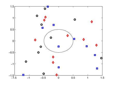
Figure 1: Random subcode construction process.

The Large Deviation Theory, which includes the Sanov theorem and the conditional limit theorem [10], addresses the probability of very non-likely events, therefore provides some of the answers. For example, the probability to generate a codeword which satisfies the hamming constraint in (2) from a uniform distribution. This probability dictates the minimum size of each random set, and obviously the minimal shaping rate $R_{s}$ required to ensure that each random set includes at least one such codeword. Furthermore, the conditional limit theorem shows that the marginals of the $N$-dimensional distribution of the selected codewords tend toward the conditional limit distribution, which is an i.i.d. distribution $q^{\star}\left(x\right)$. It is the closest distribution to $p\left(x\right)$ (in the sense of divergence) among all the distributions which satisfy the constraints.

Further, we derive achievable bounds on the transmission rate under matched and mismatched decoder. Starting with the matched decoder, one of the methods to prove achievable rate for a random ensemble of codes, which was generated according to an i.i.d. probability mass function, is the asymptotic equipartition property (AEP) theorem [10]. Since the shaping method involves codeword selection and not random generation from a target distribution, we derive a modified AEP theorem. We bound the probability to generate a codeword via this codebook construction using the conditional limit distribution. The requirement that each codeword satisfies the constraints is stronger than the requirement that the whole codebook satisfies the constraints in average; since a small amount of codewords which do not satisfy the constraints do not effect the average. Thus, the codebooks that are shaped using this methods are a subset of the codebooks which satisfy the constraints in average. Nevertheless under matched decoding, this code construction may achieve the same rate as a code which was generated i.i.d. according to $q^{\star}\left(x\right)$, i.e., the mutual information $I_{q^{\star}}\left(X;Y\right)$. This property is shown using the modified AEP.

Note that the rate achieved by the matched decoder is usually not the channel capacity since $q^{\star}\left(x\right)$ is generally not the distribution that maximizes the mutual information. For example, it can be easily shown that using an i.i.d. uniform distribution for the large code, the conditional limit distribution $q^{\star}\left(x\right)$ maximizes the entropy of the input and not the mutual information. Hence, $q^{\star}\left(x\right)$ achieves only the lower bound on the capacity subject to the constraints. Although it is only a lower bound, usually it is quite tight. This conjecture is based of the tightness of this bound for the single letter average power constraint over the AWGN channel. This can be verified using the modified BAA [8], since simulations show that the loss in rate due to the suboptimal distribution is insignificant in all SNR regions.

Next, we derive two novel lower bounds on the capacity under mismatched decoding. The first is based upon Gallager’s random exponent. The key here is to perform maximum likelihood decoding using the entire codebook, while taking into account that only a subcode was transmitted and the true distribution of the transmitted codewords. Based on this analysis, we redefine the average error probability and present a new error exponent. Using the new error exponent, we show achievable rate for the mismatched decoder. Our second bound is based upon a modified version of the joint-typicality decoder. This original decoder is not suitable for non-typical codewords, since it declares an error when the input or the output is not typical. Thus, we define a Modified-Joint-Typicality (MJT) decoder, which decodes solely based upon joint typicality between the input and the output with respect to the large codebook distribution. It might seem surprising that decoding according to a wrong distribution works and indeed this bound is correct in special cases only. One of them is uniform distribution of the large codebook and additive channels. Therefore, the AWGN channel can be treated using this approach and MJT bound can be obtained.

We show result for several examples: PAM with power constraints over AWGN, BSC and BNSC with hamming constraints. Our bounds show that for PAM over the AWGN channel there is no significant loss due to mismatch decoding. Thus, shaping gain can be attained even under mismatched decoding. This conclusion actually justifies the works of Forney and others (unknowingly), who used mismatched decoding. The BSC channel is an example where the naive approach works and coincides with our bounds. It is known that the BSC capacity is attained for uniform input probability mass function, and that linear codes achieve the BSC capacity. Such codes have the same distance spectrum for all the codewords and therefore the same error probability. In particular, the error probability of the non-typical codewords equals to the error probability of the typical. In this special case, the large codebook performance is the same as the shaped code. This example provides some insight to why the naive approach is correct for BSC.

The paper is organized as follows. Section II presents some of the preliminary background in Large Deviations and Method of Types. Section III presents our subcode construction method and the summary of the main results of this paper. Including the minimal shaping rate required for this code construction is presented in Theorem 5. It also addresses decoder types and examples of related practical shaping schemes. Section IV analyzes the matched decoder. Its significant contribution is the modified AEP theorem, which is necessary to establish the achievable rate under matched decoding. Section V analyzes the mismatched decoder and presents two achievable bounds, the MJT bound and the Gallager bound. Section VI is dedicated to examples of channels and constraints, such as BSC and AWGN subject to average power constraints.

II Preliminaries

Let capital letters denote random variables and vectors. Let small and calligraphic letters denote their realizations and support, respectively. Bold letters represent vectors. Let $X$ be a random variable with probability mass function $p\left(x\right)$ and support $\mathcal{X}$. Let $p\left(y\mid x\right)$ be a discrete memoryless channel and $Y$ be a random variable with probability mass function $p\left(y\right)$ and support $\mathcal{Y}$, such that $X$ and $Y$ are the input and output to the channel, respectively. The joint probability mass function of $\left(X,Y\right)$ is $p\left(x,y\right)$. For the sake of completeness, we repeat several basic quantities, which can be found in [10]. Thus, the entropy of the variable $X$ is

$$H_{p}\left(X\right)=-\sum_{x\in\mathcal{X}}p\left(x\right)\log p\left(x\right),$$ (3)

the conditional entropy of $Y$ given $X$ is

$$H_{p}\left(Y\mid X\right)=-\sum_{x\in\mathcal{X},y\in\mathcal{Y}}p\left(x,y\right)\log p\left(y\mid x\right)$$ (4)

and the mutual information of $\left(X,Y\right)$ is

$$I_{p}\left(X;Y\right)=H_{p}\left(Y\right)-H_{p}\left(Y\mid X\right).$$ (5)

The mutual information has also other formulations. Furthermore, let $q\left(x\right)$ be another probability mass function on the same support $\mathcal{X}$. The Kullback-Leibler information divergence (also relative entropy) between $p\left(x\right)$ and $q\left(x\right)$ (not symmetric) is

$$D\left(q\left(X\right)\parallel p\left(X\right)\right)=\sum_{x\in\mathcal{X}}q\left(x\right)\log\frac{q\left(x\right)}{p\left(x\right)},$$ (6)

using the conventions that $0\log\frac{0}{0}=0$, $0\log\frac{0}{q}=0$ and $p\log\frac{p}{0}=\infty$.

Next we review several definitions and theorems from the AEP [10, Chapters 3,7].

Definition 2.

The typical set $A_{\epsilon,p\left(x\right)}^{(N)}$ with respect to the probability mass function $p\left(x\right)$ is the set of sequences $\boldsymbol{x}\in\mathcal{X}^{N}$ with length $N$ and empirical entropies $\epsilon$-close to the true entropy $H_{p}\left(X\right)$:

$$A_{\epsilon,p\left(x\right)}^{(N)} = \left\{\boldsymbol{x}\in\mathcal{X}^{N}:\right.$$ (7)

$$\left.\left|-\frac{1}{N}\log p(\boldsymbol{x})-H_{p}\left(X\right)\right|<\epsilon\right\}.$$

The AEP theorem [10, Theorem 3.1.1], shows that if $\boldsymbol{X}$ are sequences of length $N$ drawn i.i.d. according to $p\left(x\right)$, then:

$$\Pr\left(\boldsymbol{X}\in A_{\epsilon,p\left(x\right)}^{(N)}\right) > 1-\epsilon,$$ (8)

for sufficiently large $N$.

Definition 3.

The jointly typical set $A_{\epsilon,p\left(x,y\right)}^{(N)}$ with respect to the probability mass function $p\left(x,y\right)$ is the set of sequences $(\boldsymbol{x},\boldsymbol{y})\in\mathcal{X}^{N}\times\mathcal{Y}^{N}$ with length $N$ and empirical entropies $\epsilon$-close to the true entropies:

$$A_{\epsilon,p\left(x,y\right)}^{(N)} = \left\{(\boldsymbol{x},\boldsymbol{y})\in\mathcal{X}^{N}\times\mathcal{Y}^{N}:\right.$$ (9)

$$\;\left|-\frac{1}{N}\log p(\boldsymbol{x})-H_{p}\left(X\right)\right|<\epsilon,$$

$$\;\left|-\frac{1}{N}\log p(\boldsymbol{y})-H_{p}\left(Y\right)\right|<\epsilon,$$

$$\left.\left|-\frac{1}{N}\log p(\boldsymbol{x},\boldsymbol{y})-H_{p}\left(X,Y\right)\right|<\epsilon\right\}.$$

The Joint AEP theorem [10, Theorem 7.6.1], shows that if $\left(\boldsymbol{X},\boldsymbol{Y}\right)$ are sequences of length $N$ drawn i.i.d. according to $p\left(x,y\right)$, then:

$$\Pr\left(\left(\boldsymbol{X},\boldsymbol{Y}\right)\in A_{\epsilon,p\left(x,y\right)}^{(N)}\right) > 1-\epsilon,$$ (10)

for sufficiently large $N$.

We also repeat some definitions and theorems from the Method of Types given in [10, Chapter 11].

Definition 4.

The type $P_{\boldsymbol{x}}$ of a sequence $\boldsymbol{x}=\left(x_{1},\ldots,x_{N}\right)$ is the relative proportion of occurrences of each symbol of $\mathcal{X}$, i.e., $P_{\boldsymbol{x}}\left(a\right)=N\left(a\mid\boldsymbol{x}\right)/N$ for all $a\in\mathcal{X}$, where $N\left(a\mid\boldsymbol{x}\right)$ is the number of times the symbol $a$ occurs in the sequence $\boldsymbol{x}\in\mathcal{X}^{N}$.

Let $\mathcal{P}_{N}$ be the set of types with denominator $N$ (all possible types when the sequences have length $N$). Hence, if $P\in\mathcal{P}_{N}$ the type class $T\left(P\right)$ is the set of sequences of length $N$ and type $P$, i.e.,

$$T\left(P\right)=\left\{\boldsymbol{x}\in\mathcal{X}^{N}:\;P_{\boldsymbol{x}}=P\right\}.$$ (11)

The following properties are established in [10, Theorems 11.1.2 - 11.1.4]:

1. If $\boldsymbol{X}=\left(X_{1},\ldots,X_{N}\right)$ are drawn i.i.d. according to $p\left(x\right)$, the probability of $\boldsymbol{x}$ depends only on its type and is given by

   $$p^{N}\left(\boldsymbol{x}\right)=2^{-N\left(H\left(P_{\boldsymbol{x}}\right)+D(P_{\boldsymbol{x}}\parallel p\left(X\right))\right)}.$$ (12)

2. For any type $P\in\mathcal{P}_{N}$,

   $$\frac{2^{NH\left(P\right)}}{\left(N+1\right)^{\left|\mathcal{X}\right|}}\leq\left|T\left(P\right)\right|\leq 2^{NH\left(P\right)}.$$ (13)

3. For any type $P\in\mathcal{P}_{N}$ and probability mass function $p\left(x\right)$, the probability of type class $T\left(P\right)$, where the sequences are drawn according to i.i.d. $p\left(x\right)$ is given by

   $$\frac{2^{-ND(P\parallel p\left(X\right))}}{\left(N+1\right)^{\left|\mathcal{X}\right|}}\leq p^{N}\left(T\left(P\right)\right)\leq 2^{-ND(P\parallel p\left(X\right))}.$$ (14)

The Sanov Theorem [10, Theorem 11.4.1] is part of the Large Deviation Theory, which addresses the probability of very non-likely events. The theorem is formulated as follows; let $\boldsymbol{X}=\left(X_{1},\ldots,X_{N}\right)$ be drawn i.i.d. according to $p\left(x\right)$. Let $E\subseteq\mathcal{P}$ be a set of probability mass functions. Then, the probability that $P_{\boldsymbol{X}}$ belongs to the set $E\cap\mathcal{P}_{N}$ is

$$p^{N}\left(E\right) = p^{N}\left(E\cap\mathcal{P}_{N}\right)$$ (15)

$$\leq \left(N+1\right)^{\left|\mathcal{X}\right|}2^{-ND\left(q^{\star}\left(X\right)\parallel p\left(X\right)\right)},$$

where

$$q^{\star}\left(x\right)=\arg\min_{P\left(x\right)\in E}D\left(P\left(X\right)\parallel p\left(X\right)\right)$$ (16)

is the probability mass function in $E$ that is closest to $p\left(x\right)$ in relative entropy. This is the conditional limit distribution with respect to $p\left(x\right)$ and $E$. If, in addition, the set $E$ is the closure of its interior, then

$$\lim_{N\rightarrow\infty}\frac{1}{N}\log p^{N}\left(E\right)=-D\left(q^{\star}\left(X\right)\parallel p\left(X\right)\right).$$ (17)

The conditional limit theorem [10, Theorem 11.6.2] strengthens the Sanov theorem by showing that with high probability the types of the sequences which belong to $E$ are very close to $q^{\star}\left(x\right)$ in divergence, and the marginals tend towards $q^{\star}\left(x\right)$ when $N\rightarrow\infty$. The theorem is formulated as follows. Let $E$ be a closed convex subset of $\mathcal{P}$ and let $p\left(x\right)$ be a probability mass function not in $E$. Let $X_{1},\ldots,X_{N}$ be discrete random variables drawn i.i.d. according to $p\left(x\right)$. Let $q^{\star}\left(x\right)$ achieve $\min_{P\left(x\right)\in E}D\left(P\left(X\right)\parallel p\left(X\right)\right)$. Then,

$$\lim_{N\rightarrow\infty}\Pr\left(X_{k}=a\mid P_{\boldsymbol{X}}\in E\right)=q^{\star}\left(a\right),$$ (18)

where $a\in\mathcal{X}$ and $1\leq k\leq N$.

III Shaped code construction

As stated in the introduction, the goal is approaching the channel capacity subject to a set of single letter constraints. Maximizing the average mutual information subject to these constraints obtains the maximal achievable transmission rate.

Let $X$ and $Y$ be the input and output of a memoryless channel with probability mass function $p\left(y\mid x\right)$. Let $E$ be a set of probability mass functions subjected to a set of single letter constraints, given by

$$E=\left\{P:\sum_{x\in\mathcal{X}}P\left(x\right)\varphi_{l}\left(x\right)\leq\beta_{l}\right\},$$ (19)

for $l=0,\ldots,L-1$, where $E$ is the closure of its interior, $\varphi_{l}\left(x\right)$ are bounded constraint functions and $\beta_{l}$ are constraints.

It is well-known that i.i.d. input maximizes the average mutual information subject to single letter constraints. Hence, the channel capacity is

$$C_{E}=\max_{P\left(x\right)\in E}I_{P}\left(X;Y\right),$$ (20)

and the probability mass function which achieves this capacity is

$$\hat{q}\left(x\right)=\arg\max_{P\left(x\right)\in E}I_{P}\left(X;Y\right).$$ (21)

Let $R_{q}<C_{E}$ designate the desirable transmission rate. The first method to create a random codebook is directly generate $2^{NR_{q}}$ codewords according to an i.i.d. probability mass function $q\left(x\right)$, such that $R_{q}<I_{q}\left(X;Y\right)$. We refer to this method as code construction I with respect to $q\left(x\right)$. The maximal reliable transmission rate can obviously be achieved using code construction I and $\hat{q}\left(x\right)$.

Generating a practical good codebook with a specific probability mass function is not trivial. Thus, the shaping method can be used. In this method, a large codebook is generated according to an i.i.d. uniform probability mass function and then codewords which satisfy a set of constraints are chosen, creating the shaped subcode.

We generalize this method, by allowing the large codebook to be generated according to any i.i.d. probability mass function $p\left(x\right)$. We refer to this method as code construction II with respect to $p\left(x\right)$ and $E$. We are motivated to analyze code construction II, since good practical codes for uniform probability mass function are readily available, and codeword selection might be a simple procedure for a properly structured code.

More formally, let $\mathcal{C}$ be a random codebook with $2^{NR}$ codewords, referred to as the large codebook. Let $R_{s}$ be the shaping rate. Let

$$R_{q}=R-R_{s}$$ (22)

be the shaped code rate. The large codebook is the union of $2^{NR_{q}}$ random sets, with $2^{NR_{s}}$ codewords in each random set. Each codeword with length $N$ is generated according to i.i.d. probability mass function $p\left(x\right)$ on $\mathcal{X}$. A message $\boldsymbol{m}$ to be transmitted chooses the random set. Out of this random set a single codeword $\boldsymbol{X}=\left(X_{0},\ldots,X_{N-1}\right)\in\mathcal{C}$ is selected such that it satisfies the constraints

$$\frac{1}{N}\sum_{i=0}^{N-1}\varphi_{l}\left(X_{i}\right)\leq\beta_{l}\Leftrightarrow$$

$$\sum_{x\in\mathcal{X}}P_{\boldsymbol{X}}\left(x\right)\varphi_{l}\left(x\right)\leq\beta_{l}\Leftrightarrow$$

$$P_{\boldsymbol{X}}\in E\cap\mathcal{P}_{N},$$ (23)

where $P_{\boldsymbol{X}}$ is type of $\boldsymbol{X}$. A simple illustration of the selection process can be seen in Fig. 1.

The following are examples of constraints and selection metrics. The first is the average power constraint with power limitation of $\beta_{0}$

$$\sum_{x\in\mathcal{X}}P\left(x\right)\left|x\right|^{2}\leq\beta_{0},$$ (24)

using $\varphi_{0}\left(x\right)=\left|x\right|^{2}$. The selected codewords have to satisfy $\frac{1}{N}\sum_{i=0}^{N-1}\left|X_{i}\right|^{2}\leq\beta_{0}$ to ensure that the codebook satisfies the constraints in average. Another example is the hamming power constraint, where the number of ones (’1’) is limited to $\beta_{0}$, i.e.,

$$\sum_{x=0,1}P\left(x\right)x\leq\beta_{0},$$ (25)

using $\varphi_{0}\left(x\right)=x$. In this case the selected codewords have to satisfy $\frac{1}{N}\sum_{i=0}^{N-1}X_{i}\leq\beta_{0}$.

For every constraint and constraint function $\varphi\left(\cdot\right)$, the shaping rate $R_{s}$ is chosen such that a random set includes at least one suitable codeword with probability approaching 1. The union of the selected codewords is the shaped code $\mathcal{C}_{s}$. Since each selected codeword $\boldsymbol{X}\in\mathcal{C}_{s}$ satisfies the constraints, the shaped codebook satisfies the constraints in average as required by (19).

Recall that this code construction provides us with a framework for approximating the performance of practical shaping schemes using information theoretic tools. Thus, the questions in hand are how to choose the shaping rate $R_{s}$ to find such non-typical codewords, and what are the achievable rates of this codebook construction. In particular, when using the matched decoder which is aware of the selection process and the constraints, and the mismatched decoders which is aware only of the large codebook.

The next section is dedicated to the summary of the main theorems, which provides a full overview of the main results of this paper. After which the reader can safely proceed to Section VI for special case and results.

III-A Summary of the Main Results

Let the shaping code construction be code construction II. Let $R_{s}$ be the shaping rate. Given the set of constraints $E$, let

$$q^{\star}\left(x\right)=\arg\min_{P\left(x\right)\in E}D\left(P\left(X\right)\parallel p\left(X\right)\right)$$ (26)

be the conditional limit distribution. Thus, for

$$R_{s}>D\left(q^{\star}\left(X\right)\parallel p\left(X\right)\right)$$ (27)

the probability that a random set of size $2^{NR_{s}}$ has at least one codeword which satisfies the constraints approaches 1. Furthermore, the probability that each random set includes at least one such codeword, which is the probability that the shaped codebook exists, also approaches 1.

Let $R_{M}$ be the maximal achievable rate under the constraints in $E$, code construction II using $E$ and $p\left(x\right)$, and the matched decoder. Then,

$$R_{M}<\min\left\{H_{p}\left(X\right)-D(q^{\star}\left(X\right)\parallel p\left(X\right)),I_{q^{\star}}\left(X;Y\right)\right\}$$ (28)

is the achievable rate. This results from the modified AEP theorem (Theorem 8), developed in this paper with respect to code construction II.

For the mismatched decoder, let $R_{G}$ be the achievable rate resulting from the modified development of the Gallager error exponent, which suites code construction II. Thus, for the rate

$$R_{G}<\min\left\{H_{p}\left(X\right)-D(q^{\star}\left(X\right)\parallel p\left(X\right)),\right.$$

$$\left.I_{q^{\star}}\left(X;Y\right)+D\left(q^{\star}\left(Y\right)\parallel p\left(Y\right)\right)-D(q^{\star}\left(X\right)\parallel p\left(X\right))\right\}$$ (29)

the average error probability approaches 0, i.e., this is an achievable transmission rate. Furthermore, let $R_{MJT}$ be the achievable rate resulting from the modified joint typicality analysis given in Section V-B. This rate is achievable in special cases only, in particular when the conditions of Lemma 13 are satisfied. Thus in those special cases,

$$R_{MJT}<\min\left\{H_{p}\left(X\right)-D(q^{\star}\left(X\right)\parallel p\left(X\right)),\right.$$

$$\left.D\left(P^{\star}\left(X,Y\right)||p\left(X\right)q^{\star}\left(Y\right)\right)-D(q^{\star}\left(X\right)\parallel p\left(X\right))\right\}$$ (30)

is an achievable rate, where the distribution $P^{\star}\left(x,y\right)$ is given in (116). Under the conditions of Lemma 13, the maximum between the two bounds is the achievable rate. Otherwise, only the Gallager bound can be used.

The remaining of the paper is dedicated to elaborated presentation of these results, formulating theorems and proofs, and analyzing interesting and practical special cases.

III-B Shaping rate

Thus, this section is dedicated to choosing $R_{s}$. This choice has to ensure that the large codebook has the right amount of codewords to support the transmission rate $R_{q}$, i.e., that each random set of size $2^{NR_{s}}$ has at least one codeword which satisfies the constraints with very high probability. In Theorem 5, we show that in the limit, this probability approaches 1 if $R_{s}>D\left(q^{\star}\left(X\right)\parallel p\left(X\right)\right),$ where $q^{\star}\left(x\right)=\arg\min_{P\left(x\right)\in E}D\left(P\left(X\right)\parallel p\left(X\right)\right)$. The proof highly relies on the method of types and the Sanov theorem. We also prove that (32) guarantees a minimum on $R_{s}$, such that the shaped codebook (using code construction II) exists with very high probability. This is one of the main results of this paper.

Theorem 5.

Let $R_{s}$ be the shaping rate in code construction II. Let $E$ be a set of probability mass functions, which is a closure of its interior. Let $P_{s}$ designate the probability of finding at least one codeword which satisfies the constraints (type belongs to $E$) in a random set of size $2^{NR_{s}}$, generated according to i.i.d. probability mass function $p\left(x\right)$. Let $q^{\star}\left(x\right)$ be the conditional limit probability mass function with respect to $p\left(x\right)$ and $E$, which achieves $\min_{P\left(x\right)\in E}D\left(P\left(X\right)\parallel p\left(X\right)\right)$.

Then:

1. For any $\gamma$ there exists $N_{\gamma}$, such that for $N>N_{\gamma}$

   $$P_{s}\geq$$

   $$1-\left(1-\frac{2^{-N\left(D\left(q^{\star}\left(X\right)\parallel p\left(X\right)\right)+\gamma\right)}}{\left(N+1\right)^{\left|\mathcal{X}\right|}}\right)^{2^{NR_{s}}}.$$ (31)

2. For any $\delta$ and $N\rightarrow\infty$, such that

   $$R_{s} = D\left(q^{\star}\left(X\right)\parallel p\left(X\right)\right)+\delta,$$ (32)

   $P_{s}\rightarrow 1$.

3. For any $\delta$ and any finite $\rho$, such that (32) is satisfied,

   $$P_{\rho}\triangleq\left(P_{s}\right)^{2^{\rho\cdot N}}\rightarrow 1$$ (33)

   for $N\rightarrow\infty$.

Proof:

The probability that a codeword satisfies the constraints $p^{N}\left(E\right)$, is given by the Sanov theorem (15). Let $\mathcal{P}_{N}$ be the set of types with denominator $N$. Since $E$ is the closure of its interior, it follows that $E\cap\mathcal{P}_{N}$ is nonempty for $N>N_{0}$. Hence, we can find a sequence of probability mass functions $Q_{N}$ such that $Q_{N}\in E\cap\mathcal{P}_{N}$ and

$$D\left(Q_{N}\parallel p\left(X\right)\right)\rightarrow D\left(q^{\star}\left(X\right)\parallel p\left(X\right)\right),$$ (34)

since by definition $q^{\star}\left(x\right)\in E$. This means that for any $\gamma$ there exists $N_{\gamma}>N_{0}$, such that

$$D\left(Q_{N}\parallel p\left(X\right)\right)<D\left(q^{\star}\left(X\right)\parallel p\left(X\right)\right)+\gamma.$$ (35)

Thus, for $N>N_{\gamma}$

$$p^{N}\left(E\right)\geq p^{N}\left(T\left(Q_{N}\right)\right)\geq$$

$$\frac{1}{\left(N+1\right)^{\left|\mathcal{X}\right|}}2^{-ND\left(Q_{N}\parallel p\left(x\right)\right)}\geq$$

$$\frac{1}{\left(N+1\right)^{\left|\mathcal{X}\right|}}2^{-N\left(D\left(q^{\star}\left(X\right)\parallel p\left(X\right)\right)+\gamma\right)},$$ (36)

where the inequalities follow from (14) and (35). It yields that for $N>N_{\gamma}$, the probability that none of the codewords within a random set satisfies the constraints is

$$P_{f}=$$

$$\left(1-p^{N}\left(E\right)\right)^{2^{NR_{s}}}\leq$$

$$\left(1-\frac{2^{-N\left(D\left(q^{\star}\left(X\right)\parallel p\left(X\right)\right)+\gamma\right)}}{\left(N+1\right)^{\left|\mathcal{X}\right|}}\right)^{2^{NR_{s}}}.$$ (37)

Since $P_{s}=1-P_{f}$, this concludes the first part.

For any $\delta$ and the choice $R_{s}=D\left(q^{\star}\left(X\right)\parallel p\left(X\right)\right)+\delta$,

$$\log P_{f}=$$

$$2^{NR_{s}}\log\left(1-p^{N}\left(E\right)\right)\leq$$

$$-2^{N\left(D\left(q^{\star}\left(X\right)\parallel p\left(X\right)\right)+\delta\right)}p^{N}\left(E\right)=$$

$$-2^{N\left(D\left(q^{\star}\left(X\right)\parallel p\left(X\right)\right)+\delta+\frac{1}{N}\log p^{N}\left(E\right)\right)}.$$ (38)

Furthermore, according to (17) for every $\delta$ there exists $\zeta<\delta$ and $N_{\zeta}$, such that for $N>N_{\zeta}$

$$\frac{1}{N}\log p^{N}\left(E\right)\geq-D\left(q^{\star}\left(X\right)\parallel p\left(X\right)\right)-\zeta.$$ (39)

Hence for $N>N_{\zeta}$,

$$\log P_{f}\leq-2^{N\left(\delta-\zeta\right)}$$ (40)

and for $N\rightarrow\infty$, $\log P_{f}\rightarrow-\infty$. Thus $P_{f}\rightarrow 0$ and $P_{s}\rightarrow 1$. This concludes the second part.

Furthermore,

$$P_{\rho} = \left(P_{s}\right)^{2^{\rho\cdot N}}$$ (41)

$$= \left(1-P_{f}\right)^{2^{\rho\cdot N}}$$

$$= \left[\left(1-P_{f}\right)^{1/P_{f}}\right]^{2^{\rho\cdot N}P_{f}}.$$

For $N\rightarrow\infty$, since $P_{f}\rightarrow 0$, it yields that $\left(1-P_{f}\right)^{1/P_{f}}\rightarrow 1/e$. For $N>N_{\zeta}$,

$$\log 2^{NR_{q}}P_{f} = \rho\cdot N+\log P_{f}$$ (42)

$$\leq \rho\cdot N-2^{N\left(\delta-\zeta\right)}.$$

This yields that for $N\rightarrow\infty$, $\log 2^{\rho\cdot N}P_{f}\rightarrow-\infty$ and therefore $2^{\rho\cdot N}P_{f}\rightarrow 0$. Hence, $P_{\rho}\rightarrow 1$. ∎

Thus, we found the shaping rate which ensures that a random set has at least one suitable codeword. Since the random sets are drawn independently, the probability that each one of the random sets has at least one suitable codeword is $P_{\mathcal{C}_{s}}=\left(P_{s}\right)^{2^{NR_{q}}}$. Using the last theorem with $\rho=R_{q}$, we conclude that $P_{\mathcal{C}_{s}}\rightarrow 1$, i.e., the shaped codebook (code construction II) exists with high probability.

III-C Number of codewords

In the previous section we have shown that using a large code with code rate $R$ and redundancy shaping rate $R_{s}$ a shaped subcode can be obtained. This subcode consists of $2^{N\left(R-R_{s}\right)}$ codewords which satisfy the constraints with probability tending towards 1. Hence, the maximal number of codewords in the subcode is

$$R_{q} < H_{p}\left(X\right)-D(q^{\star}\left(X\right)\parallel p\left(X\right))$$

$$\leq H_{q^{\star}}\left(X\right).$$

The last inequality follows since the number of chosen codewords can not exceed the size of the typical set of $q^{\star}\left(x\right)$. This property holds as long as $p\left(x\right)\notin E$. Whereas for $p\left(x\right)\in E$, the codewords of the large code satisfy the constraints and $R_{s}=0$.

We conclude that the achievable rate would be the minimum between the number of codewords and the rate which achieves average error probability tending towards zero for $N\rightarrow\infty$ . To establish this rate we analyze the performance of several decoders, which are presented next.

III-D Decoder types

Following our codebook construction method, we consider two types of decoders. The first is the matched decoder, which is aware of the codebook set $\mathcal{C}_{s}$ and performs optimal decoding. The second decoder is the mismatched decoder, which is only aware of the large code $\mathcal{C}$ and performs optimal decoding as if all codewords of $\mathcal{C}$ might have been transmitted. This decoder is suboptimal, but occasionally more practical than the matched decoder. In the practical special case where the large codebook is uniform code, the mismatched decoder is readily available while the adaptation to the set $\mathcal{C}_{s}$ might be extremely complex.

The achievable rate of code construction I is known. It is the mutual information related to the probability mass function which generated the codebook and the probability mass function of the channel. The achievable rate of code construction II decoded with the matched decoder, however, is an open question. It is the objective of Section IV to show that the achievable rate, in this case, is bounded by $I_{q^{\star}}\left(X;Y\right)$.

On first look, mismatch performance analysis seems as a trivial exercise. The transmitted codeword is part of the large codebook and therefore the large code performance can be used. This is the naive approach. This type of assumption was taken (without being mentioned) by Forney [1], using a decoder which is unaware of the selection process and stating that the performance and complexity of their decoder are not affected by shaping. A more careful inspection, however, reveals that the large code performance assumes the transmission of the typical codewords, while we transmit only non-typical codewords. These codewords may have worse distance spectrum towards their neighbors.

The average error probability of the large codebook tends towards zero when $R<I_{p}\left(X;Y\right)$. Thus, the bound on $R_{q}$ using the naive approach is

$$R_{n}\triangleq R_{q} < I_{p}\left(X;Y\right)-R_{s}$$ (44)

$$= I_{p}\left(X;Y\right)-D\left(q^{\star}\left(X\right)\parallel p\left(X\right)\right).$$

This bound is achievable in special cases only, for example the BSC channel, as will be shown. This is also correct for codes (bad codes), which operate at working point that justifies the approximation of minimum distance, and this justifies the analysis of Forney. Another interesting special case is a large code construction in which all words have the same distance spectrum. Obviously in such case the selection of specific codewords will not make a difference. For the AWGN, geometrically uniform (GU) codes (e.g. linear codes over rings) are known only to MPSK constellation. This raises an interesting open question: is the mismatched approximation accurate for MPSK? We know that GU codes generate good codes, and we can use them for the large uniform codebook. If the conditional limit theorem holds for GU codes over MPSK, then we can also know the choice of $R_{s}$ that will generate enough codewords that satisfy the constraints.

III-E Related practical schemes

The described random shaping code construction method highly resembles existing practical schemes. Since well-known good codes (e.g. convolutional codes, LDPC, block codes) typically generate uniform probability mass function, combined with a selection process the outcome is a shaped subcode. Our results are bounds on the performance of random constructions which approximate practical systems, which are approached using uniform i.i.d. probability mass function, the right shaping rate $R_{s}$ and sufficiently large $N$. Next we present two examples of such practical schemes.

III-E1 TS - Sign Bit Shaping

The trellis shaping [1], is a sequence oriented approach.

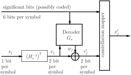
Figure 2: Bit Sign Shaping

The main idea is to use a trellis shaping code to create equivalence classes of coded sequences and then perform the shaping operation by choosing the minimum power sequence to be transmitted within each equivalence class. Sign Bit Shaping (SBS), is a special case of TS. In SBS, two bits per symbol $v_{i}=(v_{i_{1}},v_{i_{2}})$ are modified by rate 1/2 trellis shaping code, having generating matrix $\boldsymbol{G}_{s}$ and parity check matrix $\boldsymbol{H}_{s}$.

Let $N$ be the codeword length (symbols), $M$ be the number of bits represented by each symbol and $f\left(\cdot\right)$ be a mapping function to the euclidean space. Each symbol has $M-2$ unshaped bits, possibly coded by a channel code $C_{c}$ with rate $R_{c}$, and two shaped sign bits, as shown in Fig. 2. The sign bit sequence is

$$\boldsymbol{v}=\boldsymbol{s}\cdot\left(\boldsymbol{H}_{s}^{-1}\right)^{T},$$ (45)

where $\boldsymbol{s}$ are $N$ information bits. The trellis decoder creates an equivalence class

$$\left\{\boldsymbol{v}^{\prime}\right\}=\boldsymbol{v}+\left\{\boldsymbol{w}\right\},$$ (46)

where $\left\{\boldsymbol{w}\right\}=\boldsymbol{d}\boldsymbol{G}_{s}$ and $\boldsymbol{d}\in\left\{0,1\right\}^{N}$ represents all binary sequences of length $N$.

The bits are mapped into equivalence class of symbols $\left\{\boldsymbol{x}^{\prime}\right\}=f\left(\left\{\boldsymbol{v}^{\prime}\right\},\boldsymbol{u}\right)$. In this scheme the goal is power minimization; therefore the trellis decoder transmits the codeword with the minimal energy within the equivalence class, i.e.,

$$\boldsymbol{x}=\arg\min_{\left\{\boldsymbol{x}^{\prime}\right\}}\left\{\left|\boldsymbol{x}^{\prime}\right|^{2}\right\},$$ (47)

or the minimal average energy

$$\boldsymbol{x}=\arg\min_{\left\{\boldsymbol{x}^{\prime}\right\}}\left\{\frac{1}{N}\sum_{i=0}^{N-1}\left|x_{i}^{\prime}\right|^{2}\right\}.$$ (48)

Therefore, the total information rate of this scheme is

$$R_{q}=R_{c}\left(M-2\right)+1$$ (49)

bits per symbol and the shaping rate is $R_{s}=1$.

The decoding process is within the large codebook, which includes all the equivalence classes. Once the codeword $\hat{\boldsymbol{x}}$ has been decoded, the demapper extracts the shaped bits and the only additional operation required is reconstruction the shaped bits by

$$\hat{\boldsymbol{s}}=\boldsymbol{H}_{s}\left(\boldsymbol{v}+\boldsymbol{d}\boldsymbol{G}_{s}\right)=\boldsymbol{s}.$$ (50)

This operation is error free in case the entire codeword was decoded correctly ($\boldsymbol{x}=\hat{\boldsymbol{x}}$) and since $\boldsymbol{H}_{s}\cdot\boldsymbol{G}_{s}=0$.

The selection process in this scheme is to choose the codeword with the minimal average power in each equivalence class, as given in (48). For very large $N$, we claim that this selection is equivalent to selecting a sequence which satisfies the power constraint

$$\boldsymbol{x}:\;\frac{1}{N}\sum_{i=0}^{N-1}\left|x_{i}^{\prime}\right|^{2}\leq\beta_{0}.$$ (51)

Since the shaping rate $R_{s}$ is set by the shaping code $\boldsymbol{G}_{s}$ and the constraint metric $\varphi\left(x\right)=\left|x\right|^{2}$ is given, there exists minimal $\beta_{0}$ such that each equivalence class has at least one such codeword. This is dual to choosing a constraint and finding the minimal $R_{s}$ for this constraint. The constraint in turn, defines the probability mass function of the selected codewords. Recall that these sequences are very close to $q^{\star}\left(x\right)$ in distribution. The minimum average energy codeword also satisfies the constraint, thus it is one of the codewords in the previous method. Although, the chosen codewords might differ, using the different methods, the outcome is the same. A code which satisfies the constraint and is very close to $q^{\star}\left(x\right)$. Thus, choosing the minimum and choosing the codeword satisfying the minimal $\beta_{0}$ is asymptotically the same. Assuming that the large codebook is uniformly distributed, $q^{\star}\left(x\right)$ is the entropy maximizing Maxwell-Boltzmann probability mass function [10].

Note that in case of several constraints the methods are not longer equivalent since several constraints can not be represented by single metric, which can be minimized using the TS decoder at the transmitter.

III-E2 Compound LDGM-LDPC

Another example to the selection process is the scheme in [7], which was originally designed for dirty paper coding. This scheme creates a shaping code $\Lambda_{s}\left(\boldsymbol{m}\right)$ for each transmitted message $\boldsymbol{m}$ of length $NR$ using

$$\Lambda_{s}\left(\boldsymbol{m}\right) = \left\{\boldsymbol{c}=\boldsymbol{b}\boldsymbol{G}|\boldsymbol{b}\in\left\{0,1\right\}^{NR_{b}},\right.$$ (52)

$$\left.\boldsymbol{b}\boldsymbol{H}_{p}^{T}=\boldsymbol{p},\,\boldsymbol{b}\boldsymbol{H}_{m}^{T}=\boldsymbol{m}\right\},$$

where $\boldsymbol{G}$ is a sparse generation matrix, $\boldsymbol{H}_{p}$ and $\boldsymbol{H}_{m}$ are sparse parity check matrices, and $\boldsymbol{p}$ is a fixed binary sequence of length $NR_{p}$. In this nested LDGM-LDPC scheme the matrix $\boldsymbol{G}$ is designed to make the shaping code $C_{s}\left(\boldsymbol{m}\right)$ a good source code and thus suitable for average power shaping. The matrices $\boldsymbol{H}_{p}$ and $\boldsymbol{H}_{m}$ embed information and obtain good channel code properties. The encoder, given the information massage $\boldsymbol{m}$, performs a mean square error (MSE) quantization of a scaled interference (according to the dirty paper scheme) using a lattice $\Lambda_{s}\left(\boldsymbol{m}\right)+2\mathbb{Z}^{N}$ and transmits the quantization error. A special use of this scheme is the quantization of a zero interference, which results in transmitting a minimum energy codeword in the shaping code for each message. The union of the shaping codes is the large codebook and the subcode $C_{s}$ is the union of all minimum energy codewords selected from each shaping code $\Lambda_{s}\left(\boldsymbol{m}\right)$. The information rate using this scheme is $R$ and the shaping rate can be obtained from the size of the shaping code $\left|\Lambda_{s}\left(\boldsymbol{m}\right)\right|=2^{NR_{s}}$, i.e.,

$$R_{s}=R_{b}-R_{p}-R_{m}.$$ (53)

The selection process is the same as in the SBS scheme, therefore the same conclusions apply to this scheme.

IV Matched decoder: Joint Typicality Decoding

In previous sections, we discussed code construction II as a practical method to obtain a codebook which satisfies constraints. The objective of this section is showing the achievable rate of this code construction method and the matched decoder, with respect to the large codebook probability mass function $p\left(x\right)$ and the set of constraints $E$. Furthermore, we bound the $N$-dimensional distribution of the codewords, using the conditional limit distribution. These are new results, since the conditional limit theorem treated the distribution of the marginals of the selected codewords, but not the entropy rate nor the average mutual information when transmitted over a channel.

IV-A Codeword Distribution

Let $p\left(x\right)$ be i.i.d. probability mass function on $\mathcal{X}$ and let $E$ be a closed convex set such that $p\left(x\right)\notin E$. Let $q^{\star}\left(x\right)$ be the conditional limit probability mass function, which achieves $\min_{P\left(x\right)\in E}D\left(P\left(X\right)\parallel p\left(X\right)\right)$. Let us have a standard random codebook (code construction I) which uses this distribution to generate the codewords. Thus,

$$q^{\star}\left(\boldsymbol{x}\right)=\prod_{i=1}^{N}q^{\star}\left(x_{i}\right)$$ (54)

is the probability to generate the codeword $\boldsymbol{x}$ and

$$q^{\star}\left(\boldsymbol{y}\right) = \sum_{\boldsymbol{x}\in\mathcal{X}^{N}}\prod_{i=1}^{N}q^{\star}\left(x_{i}\right)p\left(y_{i}\mid x_{i}\right)$$ (55)

is the probability to generate the channel output $\boldsymbol{y}$. Let $A_{\epsilon,q^{\star}\left(X,Y\right)}^{(N)}$ designate the jointly typical set in definition 3, and let the decoder be the joint typicality decoder with respect to the i.i.d. probability mass function $q^{\star}\left(x,y\right)=q^{\star}\left(x\right)p\left(y\mid x\right)$. Let $\Pr\left\{\boldsymbol{x}\mid CC_{II}\right\}$, $\Pr\left\{\boldsymbol{y}\mid CC_{II}\right\}$ designate the probability to generate the codeword $\boldsymbol{x}$ and the channel output $\boldsymbol{y}$, respectively, using code construction II. Let $R_{s}>D\left(q^{\star}\left(X\right)\parallel p\left(X\right)\right)$. The next two lemmas upper bound $\Pr\left\{\boldsymbol{x}\mid CC_{II}\right\}$, $\Pr\left\{\boldsymbol{y}\mid CC_{II}\right\}$ using $q^{\star}\left(\boldsymbol{x}\right)$ and $q^{\star}\left(\boldsymbol{y}\right)$. These bounds are later used to derive the modified AEP theorem for code construction II (Theorem 8). The AEP, which defines the average probability of the decoding error, allows to deduct the achievable rate.

Lemma 6.

For every $\delta$ there exists $N_{\delta}$ such that for $N>N_{\delta}$

$$\Pr\left\{\boldsymbol{x}\mid CC_{II}\right\}\leq\left(N+1\right)^{\left|\mathcal{X}\right|}2^{N\delta}q^{\star}\left(\boldsymbol{x}\right).$$ (56)

Proof:

Since $p\left(x\right)$ is i.i.d. probability mass function on $\mathcal{X}$, the probability to generate a codeword $\boldsymbol{x}$ from probability mass function $p\left(x\right)$ is

$$p^{N}\left(\boldsymbol{x}\right)=2^{-N\left(H\left(Q_{\boldsymbol{x}}\right)+D\left(Q_{\boldsymbol{x}}\parallel p\left(X\right)\right)\right)},$$ (57)

where $Q_{\boldsymbol{x}}$ is the type of $\boldsymbol{x}$. The probability to generate the codeword $\boldsymbol{x}$, using code construction II, is

$$\Pr\left\{\boldsymbol{x}\mid CC_{II}\right\}=\left\{\begin{array}[]{cc}\frac{2^{-N\left(H\left(Q_{\boldsymbol{x}}\right)+D\left(Q_{\boldsymbol{x}}\parallel p\left(X\right)\right)\right)}}{p^{N}\left(E\right)},&Q_{\boldsymbol{x}}\in E,\\ 0,&Q_{\boldsymbol{x}}\notin E,\end{array}\right.$$ (58)

where $p^{N}\left(E\right)$ is the probability of the event $Q_{\boldsymbol{X}}\in E$, when generating from i.i.d. $p\left(x\right)$. Since $E$ is a closed convex set, (36) applies. Furthermore, by Pythagorean theorem for divergence [10, Theorem 11.6.1], every $P\in E$ satisfies

$$D\left(P\parallel p\left(X\right)\right)\geq D\left(P\parallel q^{\star}\left(X\right)\right)+D\left(q^{\star}\left(X\right)\parallel p\left(X\right)\right),$$ (59)

if $E$ is a closed convex set and $p\left(x\right)\notin E$. Thus,

$$\Pr\left\{\boldsymbol{x}\mid CC_{II}\right\}\leq$$

$$\frac{2^{-N\left(H\left(Q_{\boldsymbol{x}}\right)+D\left(Q_{\boldsymbol{x}}\parallel q^{\star}\left(X\right)\right)+D\left(q^{\star}\left(X\right)\parallel p\left(X\right)\right)\right)}}{p^{N}\left(E\right)}\leq$$

$$\left(N+1\right)^{\left|\mathcal{X}\right|}2^{-N\left(H\left(Q_{\boldsymbol{x}}\right)+D\left(Q_{\boldsymbol{x}}\parallel q^{\star}\left(X\right)\right)-\delta\right)},$$ (60)

using (36) and (59).

The probability to generate the codeword $\boldsymbol{x}$ with respect to i.i.d. probability mass function $q^{\star}\left(x\right)$ using code construction I (according to (12)) is

$$q^{\star}\left(\boldsymbol{x}\right)=2^{-N\left(H\left(Q_{\boldsymbol{x}}\right)+D\left(Q_{\boldsymbol{x}}\parallel q^{\star}\left(X\right)\right)\right)}.$$ (61)

Hence, we conclude that $\forall\delta$ there exists $N_{\delta}$ such that for $N>N_{\delta}$

$$\Pr\left\{\boldsymbol{x}\mid CC_{II}\right\}\leq\left(N+1\right)^{\left|X\right|}2^{N\delta}q^{\star}\left(\boldsymbol{x}\right).$$ (62)

∎

Lemma 7.

For every $\delta$ there exists $N_{\delta}$ such that for $N>N_{\delta}$

$$\Pr\left\{\boldsymbol{y}\mid CC_{II}\right\}\leq\left(N+1\right)^{\left|\mathcal{X}\right|}2^{N\delta}q^{\star}\left(\boldsymbol{y}\right).$$ (63)

Proof:

The probability of $\boldsymbol{y}$ is the sum of the joint probabilities $\Pr\left\{\boldsymbol{x},\boldsymbol{y}\right\}$ over all the codewords $\boldsymbol{x}$. Thus, $\forall\delta$ there exists $N_{\delta}$ such that for $N>N_{\delta}$

$$\Pr\left\{\boldsymbol{y}\mid CC_{II}\right\}=$$

$$\sum_{\boldsymbol{x}:Q_{\boldsymbol{x}}\in E}\Pr\left\{\boldsymbol{x}\mid CC_{II}\right\}p\left(\boldsymbol{y}\mid\boldsymbol{x}\right)\leq$$

$$\sum_{\boldsymbol{x}:Q_{\boldsymbol{x}}\in E}\left(N+1\right)^{\left|\mathcal{X}\right|}2^{N\delta}q^{\star}\left(\boldsymbol{x}\right)p\left(\boldsymbol{y}\mid\boldsymbol{x}\right)\leq$$

$$\sum_{\boldsymbol{x}\in\mathcal{X}^{N}}\left(N+1\right)^{\left|\mathcal{X}\right|}2^{N\delta}q^{\star}\left(\boldsymbol{x}\right)p\left(\boldsymbol{y}\mid\boldsymbol{x}\right)=$$

$$\left(N+1\right)^{\left|\mathcal{X}\right|}2^{N\delta}q^{\star}\left(\boldsymbol{y}\right),$$ (64)

where the first inequality follows from Lemma 6. ∎

IV-B Modified AEP

One of the methods to obtain the achievable rate of a random codebook ensemble which was drawn according to an i.i.d. probability mass function is the channel coding theorem [10, Theorem 7.7.1]. It relies on the joint AEP theorem [10, Theorem 7.6.1]. The AEP establishes the probability that a codeword and a channel output are jointly typical with respect to their joint probability mass function in two cases. In case the output is a noisy version of the input and in case of two independent variables. These two probabilities are essential to analyze the average probability of error and deduct the achievable rate such that the probability of error is tending towards zero when the codewords length tends towards infinity. The decoder is the joint typicality decoder which operates as follows. An error occurs if the transmitted codeword is not jointly typical with the received sequence or when more than one codeword is jointly typical.

The AEP theorem is not suitable for code construction II, since the codewords are generated by a selection process and not randomly drawn according to an i.i.d. distribution. Nevertheless, we know that their probability mass function converges in a sense to the i.i.d. conditional limit probability mass function. Thus, we can use this conditional limit probability mass function to redefine the decoder and derive a modified AEP theorem (Theorem 8). This theorem is used to show one of the main results of this paper, that (81) is the achievable rate under matched decoder. We conclude that the same rate can be achieved either by code construction II or by random i.i.d. generation according to $q^{\star}\left(x\right)$, i.e. $I_{q^{\star}}\left(X;Y\right)$ if the large codebook is uniformly distributed. It follows that code construction II does not lose rate under matched decoding in this case.

Theorem 8.

(Joint AEP for code construction II) Let $\boldsymbol{X}$, $\boldsymbol{Y}$ be a codeword of length $N$ drawn by code construction II with respect to $E$ and the output of memoryless channel with probability mass function $p\left(y\mid x\right)$, respectively. Let $\tilde{\boldsymbol{X}}$, $\tilde{\boldsymbol{Y}}$ be a codeword and a channel output generated by code construction II with respect to $E$, which are independent. Let $A_{\epsilon,q^{\star}\left(X,Y\right)}^{(N)}$ designate the jointly typical set in definition 3, such that $q^{\star}\left(x,y\right)=q^{\star}\left(x\right)p\left(y\mid x\right)$. Then:

1. $\Pr\left\{\left(\boldsymbol{X},\boldsymbol{Y}\right)\in A_{\epsilon,q^{\star}\left(X,Y\right)}^{(N)}\right\}\rightarrow 1$ as $N\rightarrow\infty$.

2. For every $\epsilon,\delta$, the exist $N_{\epsilon},N_{\delta}$ such that for $N\geq\max\left(N_{\delta},N_{\epsilon}\right)$

   $$\Pr\left\{\left(\tilde{\boldsymbol{X}},\tilde{\boldsymbol{Y}}\right)\in A_{\epsilon,q^{\star}\left(X,Y\right)}^{(N)}\right\}\leq$$

   $$\left(N+1\right)^{2\left|\mathcal{X}\right|}2^{-N\left(I_{q^{\star}}\left(X;Y\right)-3\epsilon-2\delta\right)}.$$ (65)

Proof:

1) Since $q^{\star}(\boldsymbol{X})=\prod_{i=0}^{N-1}q^{\star}\left(X_{i}\right)$, it yields that

$$-\frac{1}{N}\log q^{\star}(\boldsymbol{X})=$$

$$-\frac{1}{N}\sum_{i=0}^{N-1}\log q^{\star}\left(X_{i}\right)=$$

$$-\sum_{x\in\mathcal{X}}Q_{\boldsymbol{X}}\left(x\right)\log q^{\star}(x)=$$

$$H_{Q_{\boldsymbol{X}}}\left(X\right)+D\left(Q_{\boldsymbol{X}}\left(X\right)\parallel q^{\star}(X)\right),$$ (66)

where $Q_{\boldsymbol{X}}$ is the type of $\boldsymbol{X}$. Thus,

$$\left|-\frac{1}{N}\log q^{\star}(\boldsymbol{X})-H_{q^{\star}}\left(X\right)\right|=$$

$$\left|H_{Q_{\boldsymbol{X}}}\left(X\right)-H_{q^{\star}}\left(X\right)+D\left(Q_{\boldsymbol{X}}\left(X\right)\parallel q^{\star}(X)\right)\right|\leq$$

$$-\left\|Q_{\boldsymbol{X}}\left(X\right)-q^{\star}\left(X\right)\right\|_{1}\log\frac{\left\|Q_{\boldsymbol{X}}\left(X\right)-q^{\star}\left(X\right)\right\|_{1}}{\left|\mathcal{X}\right|}+$$

$$+D\left(Q_{\boldsymbol{X}}\left(X\right)\parallel q^{\star}(X)\right),$$ (67)

where the last inequality follows from [10, Theorem 17.3.3] and $\left\|P_{1}-P_{2}\right\|_{1}$ is the $\mathcal{L}_{1}$ distance between probability mass functions. The conditional limit theorem [10, Theorem 11.6.2] implies that $\forall\gamma_{0}$ there exists $N_{0}$ such that for $N>N_{0}$

$$\Pr\left\{D\left(Q_{\boldsymbol{X}}\left(X\right)\parallel q^{\star}(X)\right)\geq\gamma_{0}\mid Q_{\boldsymbol{X}}\in E\right\}\leq\eta.$$ (68)

Furthermore, [10, Lemma 11.6.1] yields that

$$\frac{1}{2\ln 2}\left\|Q_{\boldsymbol{X}}\left(X\right)-q^{\star}\left(X\right)\right\|_{1}^{2}\leq D\left(Q_{\boldsymbol{X}}\left(X\right)\parallel q^{\star}(X)\right),$$ (69)

thus if $D\left(Q_{\boldsymbol{X}}\left(X\right)\parallel q^{\star}(X)\right)\leq\gamma_{0}$, the $\mathcal{L}_{1}$ distance

$$\left\|Q_{\boldsymbol{X}}\left(X\right)-q^{\star}\left(X\right)\right\|_{1}\leq\gamma_{1}=\sqrt{2\ln 2\gamma_{0}}.$$ (70)

Since $\forall\epsilon$ there exists $\gamma_{0}$ such that

$$-\gamma_{1}\log\frac{\gamma_{1}}{\left|\mathcal{X}\right|}+\gamma_{0}\leq\epsilon,$$ (71)

from (67) and (68) it yields that there exists $N_{x}$ such that for $N>N_{x}$

$$\Pr\left\{\left|-\frac{1}{N}\log q^{\star}(\boldsymbol{X})-H_{q^{\star}}\left(X\right)\right|\geq\epsilon\right\}\leq\epsilon/3.$$ (72)

In a similar manner,

$$\left|-\frac{1}{N}\log q^{\star}(\boldsymbol{Y})-H_{q^{\star}}\left(Y\right)\right|\leq$$

$$-\left\|Q_{\boldsymbol{Y}}\left(Y\right)-q^{\star}\left(Y\right)\right\|_{1}\log\frac{\left\|Q_{\boldsymbol{Y}}\left(Y\right)-q^{\star}\left(Y\right)\right\|_{1}}{\left|\mathcal{Y}\right|}$$

$$+D\left(Q_{\boldsymbol{Y}}\left(Y\right)\parallel q^{\star}(Y)\right),$$ (73)

where $Q_{\boldsymbol{Y}}$ is the type of $\boldsymbol{Y}$. Next we bound the divergence

$$D\left(Q_{\boldsymbol{Y}}\left(Y\right)\parallel q^{\star}(Y)\right)=$$

$$\sum_{y\in\mathcal{Y}}Q_{\boldsymbol{Y}}\left(y\right)\log\frac{Q_{\boldsymbol{Y}}\left(y\right)}{q^{\star}\left(y\right)}=$$

$$\sum_{y\in\mathcal{Y}}\left(\sum_{x\in\mathcal{X}}Q_{\boldsymbol{X},\boldsymbol{Y}}\left(x,y\right)\right)\log\frac{\left(\sum_{x\in\mathcal{X}}Q_{\boldsymbol{X},\boldsymbol{Y}}\left(x,y\right)\right)}{\sum_{x\in\mathcal{X}}q^{\star}\left(x,y\right)}\leq$$

$$\sum_{y\in\mathcal{Y},x\in\mathcal{X}}Q_{\boldsymbol{X},\boldsymbol{Y}}\left(x,y\right)\log\frac{Q_{\boldsymbol{X},\boldsymbol{Y}}\left(x,y\right)}{q^{\star}\left(x,y\right)}=$$

$$\sum_{y\in\mathcal{Y},x\in\mathcal{X}}Q_{\boldsymbol{X},\boldsymbol{Y}}\left(x,y\right)\log\frac{Q_{\boldsymbol{X}}\left(x\right)P_{\boldsymbol{Y}\mid\boldsymbol{X}}\left(y\mid x\right)}{q^{\star}\left(x\right)p\left(y\mid x\right)}=$$

$$D\left(Q_{\boldsymbol{X}}\left(X\right)\parallel q^{\star}\left(X\right)\right)+D\left(P_{\boldsymbol{Y}\mid\boldsymbol{X}}\parallel p\left(Y\mid X\right)\mid Q_{\boldsymbol{X}}\right),$$ (74)

where $Q_{\boldsymbol{X},\boldsymbol{Y}}$ is the joint type of $\left(\boldsymbol{X},\boldsymbol{Y}\right)$ and the inequality follows from the log sum inequality. The typicality of the channel implies that $\forall\gamma_{2}$ there exists $N_{2}$ such that for $N>N_{2}$

$$\Pr\left\{D\left(P_{\boldsymbol{Y}\mid\boldsymbol{X}}\parallel p\left(Y\mid X\right)\mid Q_{\boldsymbol{X}}\right)\geq\gamma_{2}\right\}\leq\eta.$$ (75)

Put $\gamma_{3}=\gamma_{0}+\gamma_{2}$ and $\gamma_{4}=\sqrt{2\ln 2\gamma_{3}}$. Since $\forall\epsilon$ there exists $\gamma_{0},\gamma_{2}$ such that

$$-\gamma_{4}\log\frac{\gamma_{4}}{\left|\mathcal{Y}\right|}+\gamma_{3}\leq\epsilon,$$ (76)

from (68),(73) and (75) it yields that there exists $N_{y}$ such that for $N>N_{y}$

$$\Pr\left\{\left|-\frac{1}{N}\log q^{\star}(\boldsymbol{Y})-H_{q^{\star}}\left(Y\right)\right|\geq\epsilon\right\}\leq\epsilon/3.$$ (77)

Using similar arguments, $\forall\epsilon$ there exists $N_{xy}$ such that for $N>N_{xy}$

$$\Pr\left\{\left|-\frac{1}{N}\log q^{\star}(\boldsymbol{X},\boldsymbol{Y})-H_{q^{\star}}\left(X,Y\right)\right|\geq\epsilon\right\}\leq\epsilon/3.$$ (78)

Thus, $\forall\epsilon$ there exists $N_{\epsilon}>\max\left\{N_{x},N_{y},N_{xy}\right\}$, such that

$$\Pr\left\{\left(\boldsymbol{X},\boldsymbol{Y}\right)\in A_{\epsilon,q^{\star}\left(X,Y\right)}^{(N)}\right\}\geq 1-\epsilon.$$ (79)

This concludes the proof of first property.

2) If $\tilde{\boldsymbol{X}}$, $\tilde{\boldsymbol{Y}}$ are independent, then for $N\geq\max\left(N_{\delta},N_{\epsilon}\right)$

$$\Pr\left\{\left(\tilde{\boldsymbol{X}},\tilde{\boldsymbol{Y}}\right)\in A_{\epsilon,q^{\star}\left(X,Y\right)}^{(N)}\right\}=$$

$$\sum_{\left(\boldsymbol{x},\boldsymbol{y}\right)\in A_{\epsilon,q^{\star}}^{(N)}}\Pr\left\{\boldsymbol{x}\mid CC_{II}\right\}\Pr\left\{\boldsymbol{y}\mid CC_{II}\right\}\leq$$

$$\sum_{\left(\boldsymbol{x},\boldsymbol{y}\right)\in A_{\epsilon,q^{\star}}^{(N)}}\left(N+1\right)^{2\left|\mathcal{X}\right|}2^{N2\delta}q^{\star}\left(\boldsymbol{x}\right)q^{\star}\left(\boldsymbol{y}\right)\leq$$

$$\left(N+1\right)^{2\left|\mathcal{X}\right|}2^{2\delta N}2^{-N\left(I_{q^{\star}}\left(X;Y\right)-3\epsilon\right)},$$ (80)

where the first inequality follows from Lemmas 6 and 7, and the second follows from the joint AEP theorem [10, Theorem 7.6.1], with respect to the i.i.d. $q^{\star}\left(x,y\right)$. ∎

Hence, Theorem 8 established the joint AEP properties of code construction II with respect to the set $A_{\epsilon,q^{\star}\left(X,Y\right)}^{(N)}$. The joint AEP properties of code construction II are enough to show that for $R_{q}<I_{q^{\star}}\left(X;Y\right)$, the average error probability is tending towards zero with the block length. This can be shown by applying the channel coding theorem [10, Theorem 7.7.1] and the joint typicality decoder ($A_{\epsilon,q^{\star}\left(X,Y\right)}^{(N)}$) to code construction II.

According to Theorem 5, $R_{s}>D(q^{\star}\left(X\right)\parallel p\left(X\right))$ to ensure that each random set of size $2^{NR_{s}}$ includes a codeword which satisfies the constraints with very high probability. Therefore,

$$R_{M}\triangleq R_{q}<\min\left\{H_{p}\left(X\right)-D(q^{\star}\left(X\right)\parallel p\left(X\right)),I_{q^{\star}}\left(X;Y\right)\right\}$$ (81)

is an achievable rate, taking the maximal rate $R=H_{p}\left(X\right)$.

Since good codes for uniform probability mass function are readily available, the special case where the large codebook is uniformly distributed, i.e. $p\left(x\right)=1/\left|\mathcal{X}\right|,\forall x\in\mathcal{X}$, is of practical importance. It is easy to show that in this case, the conditional limit probability mass function $q^{\star}\left(x\right)$ achieves $\max_{P\left(x\right)\in E}H_{P\left(X\right)}$, i.e., maximize the entropy within $E$. It yields that,

$$R_{M}<I_{q^{\star}}\left(X;Y\right),$$ (82)

since

$$H_{p}\left(X\right)-D(q^{\star}\left(X\right)\parallel p\left(X\right))=H_{q^{\star}}\left(X\right)$$ (83)

and $H_{q^{\star}}\left(X\right)>I_{q^{\star}}\left(X;Y\right)$. This is the achievable rate under matched decoding in this special case. Since the selected codewords maximize the entropy of the input and not the mutual information, this is only a lower bound on the capacity subject to the constraints. Nevertheless, for the average power constraint on AWGN with discrete constellation, the distribution which maximizes the capacity is approximately the distribution which maximizes the entropy. This observation can be verified numerically, using the modified BAA [8]. Hence, the achievable rate is very close to the maximal rate in this special case.

V Mismatched Decoding

The previous sections treated code construction and the achievable rate under matched decoding. Recall that practical schemes, however, use a mismatched decoder from complexity considerations. This decoder is only aware of the large codebook and performs optimal decoding as if all the codewords might have been transmitted. It is suboptimal, but occasionally more practical since the adaptation to the shaped subcode might be extremely complex, and the decoder for the large code is readily available. This section analyzes the mismatched decoder beyond the naive approach, which showed that the non-typical codewords within the large codebook require special treatment. We present two novel lower bounds for the achievable rate using the mismatched decoder.

Our first lower bound is based upon Gallager’s error exponent bounding technique [11]. The key here is to perform maximum likelihood decoding using the entire codebook, while taking into account that only a subcode was transmitted and the true distribution of the transmitted codewords. Based on this analysis, we redefine the average error probability and present a new error exponent (84). It is important to note that this bound is suitable for any large codebook ensemble, as long as it is generated according to i.i.d. distribution and not necessarily a uniform distribution. Using the new error exponent, we show that (98) is an achievable rate for the mismatched decoder.

Our second lower bound is based upon the joint typicality decoder. This decoder is not suitable for non-typical codewords since it declares an error when the input or the output is not typical. Thus, we define a modified joint typicality (MJT) decoder, which decodes solely based on joint typicality between the input and the output with respect to the large codebook distribution. The MJT achievable rate bound is presented in (122). It might seems surprising that decoding according to a wrong distribution might work and indeed this bound is correct in special cases only (Lemma 13). One of them is uniform distribution of the large codebook and additive channels. Thus, the AWGN channel can be treated using this approach. More examples are shown in the sequel.

V-A Mismatched Decoding: Gallager Exponent

As already claimed, while the matched decoder achieves higher transmission rates, the mismatched decoder is more practical. In this section we use the Gallager bounding technique [11] to obtain a lower bound on the maximal achievable rate for the shaped subcode and the mismatched decoder.

The mismatched decoder in this section is the maximum likelihood decoder, which uses the entire codebook in the decoding process. The average error probability, however, is redefined (Theorem 9) to take into account the true distribution of the transmitted codewords. Thus, a new error exponent is presented. Using this error exponent, Theorem 10 shows an achievable rate for the mismatched decoder.

It is important to note that this bound is suitable for any large codebook ensemble, as long as it is generated according to i.i.d. distribution $p\left(x\right)$ and not necessarily the uniform distribution.

Theorem 9.

Let $p\left(y\mid x\right)$ be a memoryless channel probability mass function. For a given number of codewords $M=2^{NR}\geq 2$ of block length $N$. Let the large code ensemble be generated according to i.i.d. $p\left(x\right)$. Let $E$ be a closed convex set, such that $p\left(x\right)\notin E$. Let $q^{\star}\left(x\right)$ be the probability mass function which achieves $\min_{P\left(x\right)\in E}D\left(P\left(X\right)\parallel p\left(X\right)\right)$ and $R_{s}>D\left(q^{\star}\left(X\right)\parallel p\left(X\right)\right)$. Define a corresponding ensemble of subcodes, generated by code construction II with respect to $E$. Suppose that an arbitrary subcode codeword $m$, $1\leq m\leq M_{q}$, enters the encoder and that maximum-likelihood decoding using the entire code is employed. Then $\forall\delta$ there exists $N_{\delta}$ such that for $N\geq N_{\delta}$, the average probability of decoding error over this ensemble of subcodes, for any choice of $\rho$, $0\leq\rho\leq 1$, is bounded by

$$\overline{P}_{e}\left(E,p\right)\leq$$

$$\left(M-1\right)^{\rho}\left(N+1\right)^{\left|\mathcal{X}\right|}2^{N\delta}\left(\sum_{y\in\mathcal{Y}}\left(\sum_{x\in\mathcal{X}}q^{\star}\left(x\right)p\left(y\mid x\right)^{\frac{1}{1+\rho}}\right)\right.$$

$$\cdot\left.\left(\sum_{x}p\left(x\right)p\left(y\mid x\right)^{\frac{1}{1+\rho}}\right)^{\rho}\right)^{N}.$$ (84)

Proof:

Let $\overline{P}_{e,m}\left(E,p\right)$ designate the average error probability of codeword $m$, when using code construction II to create the subcode ensemble and maximum-likelihood decoding using the entire code. Let

$$q\left(\boldsymbol{x}_{m}\right)\triangleq\Pr\left\{\boldsymbol{x}_{m}\mid CC_{II}\right\}$$ (85)

denote the probability of codeword $m$ within the subcode ensemble. Let $\Pr\left\{\textrm{error}\mid m,\boldsymbol{x}_{m},\boldsymbol{y},p\left(\boldsymbol{x}\right)\right\}$ be the probability of error conditioned on codeword $m$ entering the encoder, the particular codeword $\boldsymbol{x}_{m}$, the received sequence $\boldsymbol{y}$ and $p\left(\boldsymbol{x}\right)$. Then, the average decoding error probability for the codeword $m$, when maximum-likelihood decoding using the entire code is employed, is

$$\overline{P}_{e,m}\left(E,p\right)=$$

$$\sum_{\boldsymbol{y}}\sum_{\boldsymbol{x}_{m}}q\left(\boldsymbol{x}_{m}\right)p\left(\boldsymbol{y}\mid\boldsymbol{x}_{m}\right)\Pr\left\{\textrm{error}\mid m,\boldsymbol{x}_{m},\boldsymbol{y},p\left(\boldsymbol{x}\right)\right\}.$$ (86)

Following the derivation of the Gallager error exponent (proof of [12, Theorem 5.6.1]), the probability of error given $m$, $\boldsymbol{x}_{m}$ and $\boldsymbol{y}$ is

$$\Pr\left\{\textrm{error}\mid m,\boldsymbol{x}_{m},\boldsymbol{y},p\left(\boldsymbol{x}\right)\right\}\leq$$

$$\left(M-1\right)^{\rho}\left(\sum_{\boldsymbol{x}}p\left(\boldsymbol{x}\right)\frac{p\left(\boldsymbol{y}\mid\boldsymbol{x}\right)^{\frac{1}{1+\rho}}}{p\left(\boldsymbol{y}\mid\boldsymbol{x}_{m}\right)^{\frac{1}{1+\rho}}}\right)^{\rho}.$$ (87)

By substituting (87) into (86) and recognizing that $\boldsymbol{x}_{m}$ is a dummy variable we obtain

$$\overline{P}_{e,m}\left(E,p\right)\leq\left(M-1\right)^{\rho}\cdot$$

$$\sum_{\boldsymbol{y}}\left(\sum_{\boldsymbol{x}}q\left(\boldsymbol{x}\right)p\left(\boldsymbol{y}\mid\boldsymbol{x}\right)^{\frac{1}{1+\rho}}\right)\left(\sum_{\boldsymbol{x}}p\left(\boldsymbol{x}\right)p\left(\boldsymbol{y}\mid\boldsymbol{x}\right)^{\frac{1}{1+\rho}}\right)^{\rho}.$$ (88)

Using Lemma 6, $\forall\delta$ there exists $N_{\delta}$ such that for $N\geq N_{\delta}$,

$$\Pr\left\{\boldsymbol{x}\mid CC_{II}\right\} \leq \left(N+1\right)^{\left|\mathcal{X}\right|}2^{N\delta}q^{\star}\left(\boldsymbol{x}\right)$$ (89)

$$= \left(N+1\right)^{\left|\mathcal{X}\right|}2^{N\delta}\prod_{i=0}^{N-1}q^{\star}\left(x_{i}\right).$$

This yields that,

$$\overline{P}_{e,m}\left(E,p\right)\leq\left(M-1\right)^{\rho}\left(N+1\right)^{\left|\mathcal{X}\right|}2^{N\delta}\cdot$$

$$\sum_{\boldsymbol{y}}\left(\sum_{\boldsymbol{x}}q^{\star}\left(\boldsymbol{x}\right)p\left(\boldsymbol{y}\mid\boldsymbol{x}\right)^{\frac{1}{1+\rho}}\right)\left(\sum_{\boldsymbol{x}}p\left(\boldsymbol{x}\right)p\left(\boldsymbol{y}\mid\boldsymbol{x}\right)^{\frac{1}{1+\rho}}\right)^{\rho}=$$

$$\left(M-1\right)^{\rho}\left(N+1\right)^{\left|\mathcal{X}\right|}2^{N\delta}\cdot$$

$$\left(\sum_{y}\left(\sum_{x}q^{\star}\left(x\right)p\left(y\mid x\right)^{\frac{1}{1+\rho}}\right)\left(\sum_{x}p\left(x\right)p\left(y\mid x\right)^{\frac{1}{1+\rho}}\right)^{\rho}\right)^{N},$$ (90)

where the equality follows since all the probability mass functions are independent and identically distributed. Each subcode codeword $m$ is bounded by (88), which does not depend on $m$. Thus, the average probability of decoding error is

$$\overline{P}_{e}\left(E,p\right)=\sum_{m=1}^{M_{q}}\Pr\left(m\right)\overline{P}_{e,m}\left(E,p\right)\leq$$

$$\left(M-1\right)^{\rho}\left(N+1\right)^{\left|\mathcal{X}\right|}2^{N\delta}\cdot$$

$$\left(\sum_{y}\left(\sum_{x}q^{\star}\left(x\right)p\left(y\mid x\right)^{\frac{1}{1+\rho}}\right)\left(\sum_{x}p\left(x\right)p\left(y\mid x\right)^{\frac{1}{1+\rho}}\right)^{\rho}\right)^{N},$$ (91)

and we obtain the bound. ∎

Thus, the last theorem showed the modified error exponent for the non-typical codewords. Note that the main difference in the derivation lays in (86), since the averaging is over the actual distribution of the codeword $\boldsymbol{x}_{m}$ ($\Pr\left\{\boldsymbol{x}_{m}\mid CC_{II}\right\}$) and not the typical codewords in the large codebook.

Since the number of codewords $M=2^{NR}$ exponentially depends on the large code rate $R$, $\forall\delta$ with $N\geq N_{\delta}$, the bound can be expressed as

$$\overline{P}_{e}\left(E,p\right) \leq\left(N+1\right)^{\left|\mathcal{X}\right|} 2{}^{-N\left(E_{0}\left(\rho,q^{\star},p\right)-\rho R-\delta\right)}$$

where

$$E_{0}\left(\rho,p_{1},p_{2}\right) \triangleq -\log\left(\sum_{y}\left(\sum_{x}p_{1}\left(x\right)p\left(y\mid x\right)^{\frac{1}{1+\rho}}\right)\right.$$ (92)

$$\cdot\left.\left(\sum_{x}p_{2}\left(x\right)p\left(y\mid x\right)^{\frac{1}{1+\rho}}\right)^{\rho}\right).$$

Once the error exponent is obtained, the achievable rate can be deducted. The following theorem shows the large code rate $R$, for which the average error probability is tending towards zero. This rate is later translated into an achievable transmission rate $R_{q}$, using $R=R_{q}+R_{s}$ (by code construction II).

Theorem 10.

Suppose that for every $\delta$ there exists $N\geq N_{\delta}$ such that for every $0\leq\rho\leq 1$ and $E_{0}\left(0,q^{\star},p\right)=0$,

$$\overline{P}_{e}\left(E,p\right) \leq\left(N+1\right)^{\left|\mathcal{X}\right|} 2{}^{-N\left(E_{0}\left(\rho,q^{\star},p\right)-\rho R-\delta\right)}.$$

Let

$$I_{q^{\star},p}\left(X,Y\right) = \lim_{\rho\rightarrow 0}\frac{E_{0}\left(\rho,q^{\star},p\right)}{\rho},$$ (93)

then for every $R<I_{q^{\star},p}\left(X,Y\right)$ and $N\rightarrow\infty$, the average error probability $\overline{P}_{e}\left(E,p\right)\rightarrow 0$.

Proof:

According to the limit definition, for every $\epsilon>0$ there exists $\rho>0$ such that

$$\frac{E_{0}\left(\rho,q^{\star},p\right)}{\rho}>I_{q^{\star},p}\left(X,Y\right)-\epsilon.$$ (94)

Taking $\epsilon=I_{q^{\star},p}\left(X,Y\right)-R$, this yields

$$E_{0}\left(\rho,q^{\star},p\right)-\rho R=\gamma>0.$$ (95)

Thus, for every $\epsilon$ the exists $\delta$ and the corresponding $N_{\delta}$ such that $\gamma>\delta$ and for $N\geq N_{\delta}$

$$0 \leq \lim_{N\rightarrow\infty}\overline{P}_{e}\left(E,p\right)$$ (96)

$$\leq \lim_{N\rightarrow\infty}\left(N+1\right)^{\left|\mathcal{X}\right|}2{}^{-N\left(E_{0}\left(\rho,q^{\star},p\right)-\rho R-\delta\right)}$$

$$= 0,$$

and therefore

$$\lim_{N\rightarrow\infty}\overline{P}_{e}\left(E,p\right)=0.$$

∎

Theorem 10 showed that when $R<I_{q^{\star},p}\left(X,Y\right)$, the average error probability $\overline{P}_{e}\left(E,p\right)$ tends towards zero. Furthermore, according to Theorem 5, $R_{q}<R-D\left(q^{\star}\left(X\right)\parallel p\left(X\right)\right)$. Hence, the average error probability $\overline{P}_{e}\left(E,p\right)\rightarrow 0$, for the shaped code if

$$R_{G}\triangleq R_{q}<I_{q^{\star},p}\left(X,Y\right)-D\left(q^{\star}\left(X\right)\parallel p\left(X\right)\right).$$ (97)

This is the achievable rate under the mismatched decoding using the Gallager exponent bounding technique. The closed form of $I_{q^{\star},p}\left(X,Y\right)$ is given at Appendix (167). This yield that,

$$R_{G} <\min\left\{H_{p}\left(X\right)-D(q^{\star}\left(X\right)\parallel p\left(X\right)),\right.$$ (98)

$$\left.I_{q^{\star}}\left(X;Y\right)+D\left(q^{\star}\left(Y\right)\parallel p\left(Y\right)\right)-D(q^{\star}\left(X\right)\parallel p\left(X\right))\right\}.$$

is an achievable transmission rate using the Gallager bounding technique. This relies on the average error probability and the maximal number of codewords using code construction II, which was discussed in Section III-C. We use the following lemma to verify that the mismatched decoder performs is worse than the matched.

Lemma 11.

Let $p\left(y\mid x\right)$ be memoryless channel and $p_{1}\left(x\right)$, $p_{2}\left(x\right)$ be input distributions. Let $p_{1}\left(y\right)$, $p_{2}\left(y\right)$ be the corresponding channel outputs, such that $p_{i}\left(y\right)=\sum_{x\in\mathcal{X}}p_{i}\left(x\right)p\left(y\mid x\right)$. Then,

$$D\left(p_{1}\left(Y\right)\parallel p_{2}\left(Y\right)\right)\leq D\left(p_{1}\left(X\right)\parallel p_{2}\left(X\right)\right).$$ (99)

Proof:

According to the definition of divergence

$$D\left(p_{1}\left(Y\right)\parallel p_{2}\left(Y\right)\right)=$$

$$\sum_{y\in\mathcal{Y}}p_{1}\left(y\right)\log\frac{p_{1}\left(y\right)}{p_{2}\left(y\right)}=$$

$$\sum_{y\in\mathcal{Y}}\left(\sum_{x\in\mathcal{X}}p_{1}\left(x\right)p\left(y\mid x\right)\right)\log\frac{\left(\sum_{x\in\mathcal{X}}p_{1}\left(x\right)p\left(y\mid x\right)\right)}{\left(\sum_{x\in\mathcal{X}}p_{2}\left(x\right)p\left(y\mid x\right)\right)}\leq$$

$$\sum_{y\in\mathcal{Y},x\in\mathcal{X}}p_{1}\left(x\right)p\left(y\mid x\right)\log\frac{p_{1}\left(x\right)p\left(y\mid x\right)}{p_{2}\left(x\right)p\left(y\mid x\right)}=$$

$$\sum_{x\in\mathcal{X}}p_{1}\left(x\right)\log\frac{p_{1}\left(x\right)}{p_{2}\left(x\right)}=$$

$$D\left(p_{1}\left(X\right)\parallel p_{2}\left(X\right)\right),$$ (100)

where the inequality follows from the log-sum inequality. ∎

Using $p_{1}\left(x\right)=q^{\star}\left(x\right)$ and $p_{2}\left(x\right)=p\left(x\right)$, we conclude that

$$D\left(q^{\star}\left(Y\right)\parallel p\left(Y\right)\right)\leq D\left(q^{\star}\left(X\right)\parallel p\left(X\right)\right);$$ (101)

therefore $R_{G}<I_{q^{\star}}\left(X;Y\right)$ as expected.

V-B Modified Joint Typicality Decoder

Our second lower bound for mismatched decoding is based on the joint typicality decoder analysis. In the original configuration, however, this decoder is not suitable for non-typical codewords in $\mathcal{C}$, since it declares an error when the input or the output is not typical according to $p\left(x,y\right)$. Thus, we define a modified joint typicality decoder. The MJT decoder is aware only of the large codebook $\mathcal{C}$, and decodes solely based on joint typicality between the input and the output with respect to the large codebook probability mass function $p\left(x,y\right)$. It might seems surprising that decoding according to a wrong probability mass function might work and indeed this bound is correct in special cases only. Lemma 13, provides a sufficient condition on $p\left(x\right)$ and the channel, such that the MJT decoder is applicable. We restrict our analysis to this particular case. We bound the average error probability of the shaped subcode $\mathcal{C}_{s}\in\mathcal{C}$, created by code construction II, using the MJT decoder to obtain an achievable rate.

Suppose that a codeword $\boldsymbol{X}\left(1\right)\in\mathcal{C}_{s}$ with index $m=1$ was sent through the channel and a noisy sequence $\boldsymbol{Y}$ was received. The original joint typicality decoder operates as follows; it examines all the codewords in the large codebook and establishes which codewords are jointly typical with the received sequence $\boldsymbol{Y}$. Since, $\boldsymbol{X}\left(1\right)$ and $\boldsymbol{Y}$ are typical with respect to $q^{\star}\left(x\right)$ and $q^{\star}\left(y\right)$, respectively; they are not typical with respect to $p\left(x\right)$ and $p\left(y\right)$. Therefore, the joint typicality decoder declares an error for each transmitted codeword. For this reason, the typicality of $\boldsymbol{X}\left(1\right)$ and $\boldsymbol{Y}$ with respect to $p\left(x\right)$, $p\left(y\right)$ is disregarded.

Let us define the modified joint typicality set and the modified joint typicality decoder.

Definition 12.

The modified jointly typical set $M_{\epsilon,p\left(x,y\right)}^{(N)}$ with respect to the probability mass function $p\left(x,y\right)$ is the set of sequences $(\boldsymbol{x},\boldsymbol{y})\in\mathcal{X}^{N}\times\mathcal{Y}^{N}$ with empirical entropies $\epsilon$-close to the true entropy $H_{p}\left(X,Y\right)$:

$$M_{\epsilon,p\left(x,y\right)}^{(N)} = \left\{(\boldsymbol{x},\boldsymbol{y})\in\mathcal{X}^{N}\times\mathcal{Y}^{N}:\right.$$ (102)

$$\left.\left|-\frac{1}{N}\log p(\boldsymbol{x},\boldsymbol{y})-H_{p}\left(X,Y\right)\right|<\epsilon\right\}.$$

The modified joint typicality decoder operates as follows; first it examines all the codewords in the large codebook and establishes which codewords are MJT with the received sequence $\boldsymbol{Y}$, i.e., belong to the set $M_{\epsilon,p\left(x,y\right)}^{(N)}$. An error occurs, either when the sent codeword $\boldsymbol{X}\left(1\right)$ is not MJT with the received sequence $\boldsymbol{Y}$ or when more that one codeword is MJT with $\boldsymbol{Y}$.

Let us define the event that a codeword $\boldsymbol{X}\left(i\right)\in\mathcal{C}$ is MJT with the output as $E_{i}$, $i=\left\{1,...,2^{nR}\right\}$. The event $E_{1}^{c}$ (the complete to $E_{1}$) is the first error event, i.e., the sent codeword is not MJT with the received sequence. Thus, the probability of error is therefore the union of these events. Let us now define an event $E_{Y_{q}}$, where the received sequence $\boldsymbol{Y}$ is typical with respect to the probability mass function $q^{\star}\left(y\right)$, i.e., $\boldsymbol{Y}\in A_{\epsilon,q^{\star}\left(y\right)}^{(N)}$ and $E_{Y_{q}}^{c}$ as the complete to $E_{Y_{q}}$. Using the AEP property for code construction II

$$\Pr\left\{E_{Y_{q}}^{c}\mid m=1\right\}<\frac{\epsilon}{2},$$ (103)

for sufficiently large $N$. Hence, the probability of error is bounded

$$\Pr\left\{\textrm{error}|m=1\right\}=$$

$$\Pr\left\{E_{1}^{c}\cup E_{2}\cup\cdots\cup E_{2^{nR}}|m=1\right\}=$$

$$\Pr\left\{\left(E_{1}^{c}\cup E_{2}\cup\cdots\cup E_{2^{nR}}\right)\cap E_{Y_{q}}|m=1\right\}\Pr\left\{E_{Y_{q}}|m=1\right\}+$$

$$\Pr\left\{\left(E_{1}^{c}\cup E_{2}\cup\cdots\cup E_{2^{nR}}\right)\cap E_{Y_{q}}^{c}|m=1\right\}\Pr\left\{E_{Y_{q}}^{c}|m=1\right\}\leq$$

$$\Pr\left\{\left(E_{1}^{c}\cup E_{2}\cup\cdots\cup E_{2^{nR}}\right)\cap E_{Y_{q}}|m=1\right\}+\frac{\epsilon}{2}\leq$$

$$\Pr\left\{E_{1}^{c}|m=1\right\}+\sum_{i=2}^{2^{NR}}\Pr\left\{E_{i}\cap E_{Y_{q}}|m=1\right\}+\frac{\epsilon}{2},$$ (104)

where the last inequality follows from the union bound and since $\Pr\left\{E_{1}^{c}\cap E_{Y_{q}}|m=1\right\}\leq\Pr\left\{E_{1}^{c}|m=1\right\}$.

First, we analyze $\Pr\left\{E_{1}^{c}|m=1\right\}$, which is equal to $\Pr\left\{\left(\boldsymbol{X}\left(1\right),\boldsymbol{Y}\right)\notin M_{\epsilon,p\left(x,y\right)}^{(N)}\right\}$. The following lemma introduces a sufficient condition such that this probability is sufficiently small. In the general case, however, the decoder will not choose the right codeword, since the probability of joint typicality according to a wrong probability mass function ($p\left(x,y\right)$) is extremely low.

Lemma 13.

For sufficiently large $N$

$$\Pr\left\{\left(\boldsymbol{X}\left(1\right),\boldsymbol{Y}\right)\notin M_{\epsilon,p\left(x,y\right)}^{(N)}\right\}<\epsilon$$ (105)

if

$$\log p\left(x\right)-H_{p}\left(Y\mid X=x\right)=c,\;\forall x\in\mathcal{X},$$ (106)

where $c$ is a constant.

Proof:

Since $p\left(\boldsymbol{X}\left(1\right),\boldsymbol{Y}\right)=\prod_{i=0}^{N-1}p\left(X_{i}\left(1\right),Y_{i}\right)$, it yields that

$$-\frac{1}{N}\log p\left(\boldsymbol{X}\left(1\right),\boldsymbol{Y}\right)=$$

$$-\frac{1}{N}\sum_{i=0}^{N-1}\log p\left(X_{i}\left(1\right),Y_{i}\right)=$$

$$-\sum_{x\in\mathcal{X},y\in\mathcal{Y}}Q_{\boldsymbol{X}\left(1\right),\boldsymbol{Y}}\left(x,y\right)\log p(x,y)=$$

$$-\sum_{x\in\mathcal{X},y\in\mathcal{Y}}Q_{\boldsymbol{X}\left(1\right)}\left(x\right)P_{\boldsymbol{Y}\mid\boldsymbol{X}\left(1\right)}\left(x,y\right)\log p(x,y)=$$

$$-\sum_{x\in\mathcal{X}}Q_{\boldsymbol{X}\left(1\right)}\left(x\right)\left[\log p(x)-H_{P_{\boldsymbol{Y}\mid\boldsymbol{X}\left(1\right)}}\left(Y\mid X=x\right)\right.$$

$$\left.-D\left(P_{\boldsymbol{Y}\mid\boldsymbol{X}\left(1\right)}\left(Y\mid X=x\right)\parallel p\left(Y\mid X=x\right)\right)\right],$$ (107)

where $Q_{\boldsymbol{X}\left(1\right),\boldsymbol{Y}}$ is the type of $\left(\boldsymbol{X}\left(1\right),\boldsymbol{Y}\right)$ and $P_{\boldsymbol{Y}\mid\boldsymbol{X}\left(1\right)}$ is the type of the channel, i.e., of $\boldsymbol{Y}$ given $\boldsymbol{X}\left(1\right)$. Hence,

$$\left|-\frac{1}{N}\log p\left(\boldsymbol{X}\left(1\right),\boldsymbol{Y}\right)-H_{p}\left(X,Y\right)\right|=$$

$$\left|\sum_{x\in\mathcal{X}}\left(p\left(x\right)-Q_{\boldsymbol{X}\left(1\right)}\left(x\right)\right)\left[\log p\left(x\right)-H_{p}\left(Y\mid X=x\right)\right]\right.+$$

$$\sum_{x\in\mathcal{X}}Q_{\boldsymbol{X}\left(1\right)}\left(x\right)\left[H_{P_{\boldsymbol{Y}\mid\boldsymbol{X}\left(1\right)}}\left(Y\mid X=x\right)-H_{p}\left(Y\mid X=x\right)\right.+$$

$$\left.\left.D\left(P_{\boldsymbol{Y}\mid\boldsymbol{X}\left(1\right)}\left(Y\mid X=x\right)\parallel p\left(Y\mid X=x\right)\right)\right]\right|\leq$$

$$\sum_{x\in\mathcal{X}}Q_{\boldsymbol{X}\left(1\right)}\left(x\right)\left[\left|H_{P_{\boldsymbol{Y}\mid\boldsymbol{X}\left(1\right)}}\left(Y\mid X=x\right)-H_{p}\left(Y\mid X=x\right)\right|\right.+$$

$$\left.D\left(P_{\boldsymbol{Y}\mid\boldsymbol{X}\left(1\right)}\left(Y\mid X=x\right)\parallel p\left(Y\mid X=x\right)\right)\right],$$ (108)

where the last derivation is correct since $\log p\left(x\right)-H_{p}\left(Y\mid X=x\right)=c$ for every $x\in\mathcal{X}$. Using the typicality of the channel and the same arguments as in Theorem 8, for every $\epsilon$ there exists $N_{\epsilon}$ such that for $N>N_{\epsilon}$

$$\left|H_{P_{\boldsymbol{Y}\mid\boldsymbol{X}\left(1\right)}}\left(Y\mid X=x\right)-H_{p}\left(Y\mid X=x\right)\right|+$$

$$D\left(P_{\boldsymbol{Y}\mid\boldsymbol{X}\left(1\right)}\left(Y\mid X=x\right)\parallel p\left(Y\mid X=x\right)\right)\leq\epsilon,$$ (109)

for every $x\in\mathcal{X}$ with probability larger than $1-\epsilon$. We conclude that for $N>N_{\epsilon}$

$$\Pr\left\{\left|-\frac{1}{N}\log p\left(\boldsymbol{X}\left(1\right),\boldsymbol{Y}\right)-H_{p}\left(X,Y\right)\right|>\epsilon\right\}\leq\epsilon,$$ (110)

i.e., $\Pr\left\{\left(\boldsymbol{X}\left(1\right),\boldsymbol{Y}\right)\notin M_{\epsilon,p\left(x,y\right)}^{(N)}\right\}<\epsilon$. ∎

A special case where condition (106) is satisfied is uniform probability mass function $p\left(x\right)=1/\left|\mathcal{X}\right|,\;\forall x\in\mathcal{X}$ and a channel which satisfies $H_{p}\left(Y\mid X=x\right)=c,\;\forall x$. Binary symmetric channel (BSC) and additive noise channels $Y=X+N$, are examples for which this property is satisfied. Hence, for these channels and uniformly distributed large codebook

$$\Pr\left\{E_{1}^{c}|m=1\right\}<\frac{\epsilon}{2},$$ (111)

for sufficiently large $N$.

Next we bound the probability $\Pr\left\{E_{i}\cap E_{Y_{q}}|m=1\right\}$, $i=2,\ldots,2^{nR}$. The event $E_{i}\cap E_{Y_{q}}|m=1$ is equivalent to $\left(\boldsymbol{X}\left(i\right),\boldsymbol{Y}\right)\in M_{\epsilon,p\left(x,y\right)}^{(N)}\cap A_{\epsilon,q^{\star}\left(y\right)}^{(N)}$. Since by the code generation process, $\boldsymbol{X}\left(1\right)$ and $\boldsymbol{X}\left(i\right)$ are independent for $i\neq 1$, so are $\boldsymbol{Y}$ and $\boldsymbol{X}\left(i\right)$ for $i\neq 1$. Since $\boldsymbol{X}\left(i\right)$ was generated according to i.i.d. $p\left(x\right)$ and $\boldsymbol{Y}$ was generated from code construction II

$$\Pr\left\{\boldsymbol{X}\left(i\right),\boldsymbol{Y}\right\}=p\left(\boldsymbol{X}\left(i\right)\right)\Pr\left\{\boldsymbol{Y}\mid CC_{II}\right\}.$$ (112)

Thus, using Lemma 7

$$\Pr\left\{E_{i}\cap E_{Y_{q}}|m=1\right\}=$$

$$\sum_{\left(\boldsymbol{x},\boldsymbol{y}\right)\in M_{\epsilon,p\left(x,y\right)}^{(N)}\cap A_{\epsilon,q^{\star}\left(y\right)}^{(N)}}\Pr\left\{\boldsymbol{x},\boldsymbol{y}\right\}=$$

$$\sum_{\left(\boldsymbol{x},\boldsymbol{y}\right)\in M_{\epsilon,p\left(x,y\right)}^{(N)}\cap A_{\epsilon,q^{\star}\left(y\right)}^{(N)}}p\left(\boldsymbol{x}\right)\Pr\left\{\boldsymbol{y}\mid CC_{II}\right\}\leq$$

$$\left(N+1\right)^{\left|\mathcal{X}\right|}2^{N\delta}\sum_{\left(\boldsymbol{x},\boldsymbol{y}\right)\in M_{\epsilon,p\left(x,y\right)}^{(N)}\cap A_{\epsilon,q^{\star}\left(y\right)}^{(N)}}p\left(\boldsymbol{x}\right)q^{\star}\left(\boldsymbol{y}\right)=$$

$$\left(N+1\right)^{\left|\mathcal{X}\right|}2^{N\delta}\Pr\left\{E_{i}\cap E_{Y_{q}}|m=1,CC_{I}\right\}.$$ (113)

The event $E_{i}\cap E_{Y_{q}}|m=1,CC_{I}$ is easier to analyze. It is equivalent to the event $P_{\boldsymbol{X}\left(i\right),\boldsymbol{Y}}\in\Lambda\cap\mathcal{P}_{N}\left(X,Y\right)$, where $\left(\boldsymbol{X}\left(i\right),\boldsymbol{Y}\right)$ are drawn according to i.i.d. $p\left(x\right)q^{\star}\left(y\right)$, $P_{\boldsymbol{X}\left(i\right),\boldsymbol{Y}}$ is the type of $\left(\boldsymbol{X}\left(i\right),\boldsymbol{Y}\right)$ and

$$\Lambda = \left\{P:\right.$$ (114)

$$\left|\sum_{x\in\mathcal{X},y\in\mathcal{Y}}P\left(x,y\right)\log p(x,y)-H_{p}\left(X,Y\right)\right|\leq\epsilon,$$

$$\left.\left|\sum_{x\in\mathcal{X},y\in\mathcal{Y}}P\left(x,y\right)\log q^{\star}(y)-H_{q}\left(Y\right)\right|\leq\epsilon\right\}.$$

According to Sanov’s theorem [11, Theorem 11.4.1], the probability that $\left(\boldsymbol{X}\left(i\right),\boldsymbol{Y}\right)$ has type $P_{\boldsymbol{X}\left(i\right),\boldsymbol{Y}}\in\Lambda\cap\mathcal{P}_{N}\left(X,Y\right)$ is bounded by

$$\Pr\left\{E_{i}\cap E_{Y_{q}}|m=1,CC_{I}\right\}\leq 2^{-ND\left(P^{\star}\parallel p\left(X\right)q^{\star}\left(Y\right)\right)}$$ (115)

where

$$P^{\star}\left(x,y\right)=\arg\min_{P\left(x,y\right)\in\Lambda}D\left(P\parallel p\left(X\right)q^{\star}\left(Y\right)\right).$$ (116)

To obtain the minimal divergence in $\Lambda$, we construct the following Lagrangian and its derivative

$$J\left(P\right) =D\left(P\|p\left(X\right)q^{\star}(Y)\right)$$ (117)

$$+\;\lambda_{0}\sum P\left(x,y\right)$$

$$+\;\lambda_{1}\sum P\left(x,y\right)\log q^{\star}\left(y\right)$$

$$+\;\lambda_{2}\sum P\left(x,y\right)\log p\left(x,y\right),$$

$$\frac{dJ\left(P\left(x,y\right)\right)}{dP\left(x,y\right)} =\log\frac{P\left(x,y\right)}{p\left(x\right)q^{\star}(y)}+\lambda_{0}$$ (118)

$$+\lambda_{1}\log q^{\star}\left(y\right)+\lambda_{2}\log p\left(x,y\right).$$

The solution is given in a parametric form

$$P^{\star}\left(x,y\right)=$$ (119)

$$p\left(x\right)q^{\star}(y)\exp\left(\lambda_{0}+\lambda_{1}\log q^{\star}\left(y\right)+\lambda_{2}\log p\left(x,y\right)\right),$$

where the Lagrange multipliers $\lambda_{0},\lambda_{1},\lambda_{2}$ should satisfy the constraints in (114).

Finally, by substituting (111) and (115) into (104), the error probability can be further bounded

$$\Pr\left\{\textrm{error}|m=1\right\}\leq\epsilon+2^{-N\left(D\left(P^{\star}\parallel p\left(X\right)q^{\star}\left(Y\right)\right)-R-\delta\right)}.$$ (120)

Hence, for

$$R = R_{q}+R_{s}$$ (121)

$$< D\left(P^{\star}\left(X,Y\right)||p\left(X\right)q^{\star}\left(Y\right)\right),$$

the error probability tend towards zero for $N\rightarrow\infty$. According to Theorem 5, $R_{s}>D(q^{\star}\left(X\right)\parallel p\left(X\right))$ to ensure that each random set of size $2^{NR_{s}}$ includes a codeword which satisfies the constraints with very high probability. It yields that for $N\rightarrow\infty$, the minimum between

$$R_{MJT}\triangleq R_{q}<$$

$$D\left(P^{\star}\left(X,Y\right)||p\left(X\right)q^{\star}\left(Y\right)\right)-D(q^{\star}\left(X\right)\parallel p\left(X\right))$$ (122)

and the maximal amount of codewords (III-C) is an achievable rate using this bounding technique.

VI Special cases

In the previous sections we discussed code construction II, as a method to obtain shaped codebooks. We have shown the maximal amount of the available codewords and achievable rates for the matched and the mismatched decoders. In this section we analyze several special cases. The first is the case where the large codebook is generated according to an i.i.d. uniform distribution and the channel satisfies the condition in Lemma 13. In this case, all the bounds are applicable. The more general case, where the large codebook is non-uniform, is later discusses in context of several special cases: the BNSC and AWGN with Gaussian large codebook. The details are given next.

VI-A Uniform large codebook

The special case where the large codebook is uniformly distributed on the support is of practical importance. Furthermore, although the Gallager bound can be obtained for any i.i.d. $p\left(x\right)$, the MJT bound can be obtained only when condition (106) is satisfied. In order to compare all the bounds, the following examples focus on a special case of (106), where $p\left(x\right)=1/\left|\mathcal{X}\right|$ and the channel satisfies

$$H_{p}\left(Y\mid X=x\right)=c,\;\forall x\in\mathcal{X}$$ (123)

for any $c$. In particular, we analyze the AWGN and BSC channels.

Our first observation is regarding the achievable rate for the matched decoder. It is easy to show that for uniform $p\left(x\right)$, the conditional limit probability mass function $q^{\star}\left(x\right)$ does not maximize the mutual information, but the entropy $H_{P}\left(X\right)$ within the set $E$, i.e.,

$$q^{\star}\left(x\right)=\arg\max_{P\left(x\right)\in E}H_{P}\left(X\right).$$ (124)

Thus, code construction II can not achieve the maximal rate even for the matched decoder, since generally different probability mass functions maximize the mutual information and the entropy subject to the constraints. Nevertheless, for the average power constraint over AWGN with discrete input constellation, the probability mass function which maximizes the mutual information is approximately the probability mass function which maximizes the entropy. Hence, the achievable rate is very close to the maximal rate. This can be verified using the modified BAA [8].

For the mismatched decoder, the Gallager bound takes the form of

$$R_{G}<I_{q^{\star}}\left(X;Y\right)+D\left(q^{\star}\left(Y\right)\parallel p\left(Y\right)\right)+H_{q^{\star}}\left(X\right)-\log\left|\mathcal{X}\right|,$$ (125)

since

$$D\left(q^{\star}\left(X\right)\parallel p\left(X\right)\right)=\log\left|\mathcal{X}\right|-H_{q^{\star}}\left(X\right).$$ (126)

The parametric form of the probability mass function $P^{\star}\left(x,y\right)$ of the MJT bound in (119) is also simplified into

$$P^{\star}\left(x,y\right) = \mathcal{K}q^{\star}(y)^{\tilde{\lambda}_{1}}p\left(y\mid x\right)^{\lambda_{2}},$$ (127)

where $\tilde{\lambda}_{1}=\lambda_{1}+1$, $\lambda_{2}$ and $\mathcal{K}$ (represents all the constants) satisfy the constraints in (114). There is no closed form solution in the general case and the Lagrange multipliers should be obtained numerically. Once these parameters are found, the MJT bound takes the form of

$$R_{MJT}<D\left(P^{\star}\left(X,Y\right)||p\left(X\right)q^{\star}\left(Y\right)\right)+H_{q^{\star}}\left(X\right)-\log\left|\mathcal{X}\right|.$$ (128)

The maximal amount of codewords is not a limitation in this case, since the entropy of the large codebook is $\log\left|\mathcal{X}\right|$. Thus taking the maximal $R=\log\left|\mathcal{X}\right|$, we can obtain the typical set of $q^{\star}\left(x\right)$ (up to the $\delta$), since $R_{q}<H_{q^{\star}}\left(X\right)$. For more details recall Section III-C.

VI-A1 AWGN

The first example that we analyze is the memoryless AWGN channel with uniformly distributed large codebook, which is a special case of (123). Let $\mathcal{X}$ be a discrete constellation with cardinality $\left|\mathcal{X}\right|$. Let $\boldsymbol{X}=\left(X_{0},\cdots,X_{N-1}\right)$ be a random vector of length $N$, representing the transmitted symbols, where $X_{i}\in\mathcal{X}$. We allow the amplitude levels of the constellation points to change to model an amplifier at the transmitter. This is done by multiplying the constellation by a real and positive scaling parameter $\alpha>0$. Let $\boldsymbol{Z}=\left(Z_{0},\cdots,Z_{N-1}\right)$ be an i.i.d. Gaussian noise vector, where $Z_{i}\sim\mathcal{N}(0,1)$ are i.i.d. Gaussian noise samples, normalized to unit variance. Let $\boldsymbol{Y}=\left(Y_{0},\cdots,Y_{N-1}\right)$ be the random vector at the receiver, such that

$$Y_{i}=\alpha X_{i}+Z_{i}.$$ (129)

The transmission is subject to an average power constraint, where the maximum average power allowed is $\beta_{0}$. Since the scaling of the constellation is a degree of freedom, for each scaling $\alpha$ the power constraint can be formulated as

$$E\left(\alpha\right)=\left\{P:\sum_{x\in\mathcal{X}}P\left(x\right)\varphi_{0}\left(x,\alpha\right)\leq\beta_{0}\right\},$$ (130)

using $\varphi_{0}\left(x,\alpha\right)=\alpha^{2}\left|x\right|^{2}$. The corresponding decision rule for choosing codewords is therefore

$$\frac{1}{N}\sum_{i=0}^{N-1}\left|\alpha X_{i}\right|^{2}\leq\beta_{0},$$ (131)

which is equivalent to

$$\frac{1}{N}\sum_{i=0}^{N-1}\left|X_{i}\right|^{2}\leq\beta_{0}/\alpha^{2}.$$ (132)

For example, let the constellation be $\mathcal{X}=\left\{-3,-1,1,3\right\}$ (4-PAM), and the power constraint be $\beta_{0}=5$. For each scaling $\alpha$, $E\left(\alpha\right)$ is a set of probability mass functions which satisfy the constraint. In particular, lets consider $\alpha=1,1.1,1.3$ and the corresponding sets $E\left(1\right)$, $E\left(1.1\right)$ and $E\left(1.3\right)$.

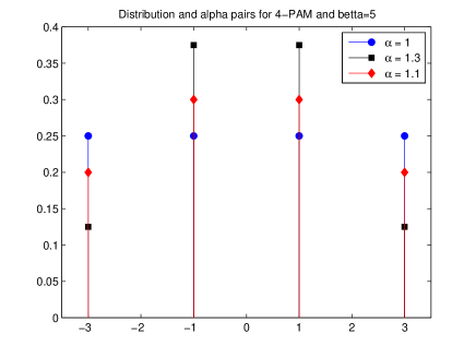
Figure 3: Probability mass functions corresponding to $\alpha=1,1.1,1.3$ and $\beta=5$.

The probability mass functions

$$p_{1} = \left(\frac{1}{4},\frac{1}{4},\frac{1}{4},\frac{1}{4}\right),$$ (133)

$$p_{1.1}=\left(\frac{2}{10},\frac{3}{10},\frac{3}{10},\frac{2}{10}\right),$$ (134)

$$p_{1.3}=\left(\frac{1}{8},\frac{3}{8},\frac{3}{8},\frac{1}{8}\right),$$ (135)

in Fig. 3 satisfy the constraints in $E\left(1\right)$, $E\left(1.1\right)$ and $E\left(1.3\right)$, respectively. It can be seen that larger scaling is required as the distribution becomes more “Gaussian”. Thus, there is a tradeoff between the scaling parameter and how much the distribution is “Gaussian” or non-uniform.

Thus, we have proved that (82), (125) and (128) are achievable rates for the matched and mismatched decoders, corresponding to large code distribution $p\left(x\right)$ and the constraints sets $E$. Since $\alpha$ is a degree of freedom, we still need to establish the optimal scaling parameter $\alpha^{\star}$, which attains the maximum of each bound. This also dictates the optimal decision rule to choose the codewords in the shaped code construction process. Hence, the achievable rate using the matched decoder is

$$R_{Mu}=\max_{\alpha}I_{q_{\alpha}^{\star}\left(x\right)}\left(X;Y\right).$$ (136)

It is also known that the Maxwell Boltzmann distribution achieves the maximal entropy subject an average power constraint [10], therefore the conditional limit probability mass function is

$$q_{\alpha}^{\star}\left(x\right)=\frac{\exp\left(-t\left|x\right|^{2}\right)}{\sum_{x^{\prime}\in\mathcal{X}}\exp\left(-t\left|x^{\prime}\right|^{2}\right)}.$$ (137)

The parameter $t$ is chosen such that the constraint is satisfied with equality, i.e.,

$$\sum_{x\in\mathcal{X}}q_{\alpha}^{\star}\left(x\right)\varphi\left(x,\alpha\right)=\beta_{0},$$ (138)

which follows from the concavity of the entropy.

The maximal rates for the mismatched Gallager and MJT bounds are also calculated with respect to the optimal $\alpha$ for each bound, such that

$$R_{Gu}<$$ (139)

$$\max_{\alpha}I_{q_{\alpha}^{\star}}\left(X;Y\right)+D\left(q_{\alpha}^{\star}\left(Y\right)\parallel p\left(Y\right)\right)+H_{q_{\alpha}^{\star}}\left(X\right)-\log\left|\mathcal{X}\right|$$

and

$$R_{MJTu}<$$ (140)

$$\max_{\alpha}D\left(P_{\alpha}^{\star}\left(X,Y\right)||p\left(X\right)q_{\alpha}^{\star}\left(Y\right)\right)+H_{q_{\alpha}^{\star}}\left(X\right)-\log\left|\mathcal{X}\right|,$$

using (137).

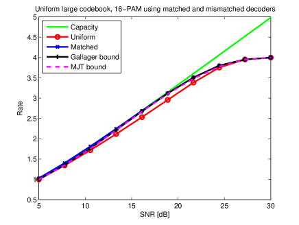
Figure 4: Achievable rates 16-PAM, AWGN

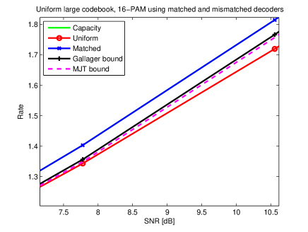
Figure 5: Achievable rates 16-PAM, AWGN, low SNR.

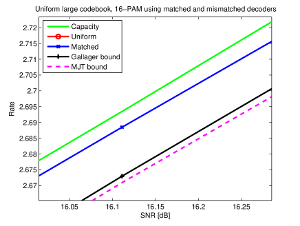
Figure 6: Achievable rates 16-PAM, AWGN, high SNR.

Figs. 4-6 present the maximal achievable rates using the matched decoder and our two lower bounds for the mismatched decoder versus SNR. The scaling parameter $\alpha$ is optimized for each bound at each SNR point. We keep the noise variance constant ($Z_{i}\sim\mathcal{N}(0,1)$) and change the transmission power $\beta_{0}$ to control the SNR. The large codebook is uniformly distributed over 16-PAM. These rates are compared to the capacity of the power constrained continuous AWGN channel, which is denoted by “Capacity”. They are further compared to the uniformly distributed 16-PAM constellation, which is denoted by “Uniform”. It can be seen that the matched decoder shaping curve is very close to the capacity curve up to the rate of 3 bps. The gap to capacity in high SNR (around 3 bps) is approximately 0.1 dB, 0.2 dB for the matched and the mismatched decoders, respectively. In low SNR the gap is approximately 0 dB, 0.3 dB for the matched and the mismatched decoders, respectively. Thus, the main conclusion from the graphs is that for PAM over AWGN there is no significant loss due to mismatched decoding, and that shaping gain can be attained. This conclusion actually justifies the works of Forney and others (unknowingly), who used mismatched decoding.

VI-A2 BSC

Our second example is the binary symmetric channel, in which the input $\mathcal{X}=\left\{0,1\right\}$ is inverted with probability $\gamma$. The mutual information of this channel is

$$I_{P}\left(X;Y\right)=H_{P}\left(Y\right)-H\left(\gamma\right),$$ (141)

where $P$ is the input probability mass function and $H\left(\gamma\right)=-\left(\gamma\log\gamma+\left(1-\gamma\right)\log\left(1-\gamma\right)\right)$.

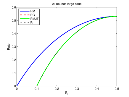
Figure 7: BSC: matched and the mismatched decoder versus $\beta_{0}$, for $\gamma=0.1$ and uniform large codebook.

This channel is another special case of (123), for $P=0.5$ (uniform large codebook). The hamming power constraint

$$\frac{1}{N}\sum_{i=0}^{N-1}X_{i}\leq\beta_{0},$$ (142)

is very common for this channel. Thus, let $E$ be the constrained probability mass functions set

$$E=\left\{P:\sum_{x\in\left\{0,1\right\}}P\left(x\right)x\leq\beta_{0}\right\},$$ (143)

where $\beta_{0}\leq\frac{1}{2}$ is the maximal number of ’1’s allowed, and let $q^{\star}\left(x\right)$ be the conditional limit probability mass function which attains minimum $D\left(P\left(X\right)\parallel p\left(X\right)\right)$ in $E$. Using the convexity of the divergence in $P\left(x\right)$, it implies that the constraint is satisfied with an equality. Thus, $q^{\star}\left(x=1\right)=\beta_{0}$. The achievable rate for the matched decoder is therefore $I_{q^{\star}}\left(X;Y\right)=H_{q^{\star}}\left(Y\right)-H\left(\gamma\right)$.

Next we obtain the achievable rates $R_{G}$ and $R_{MJT}$ for this channel, using the Gallager and the MJT bounding techniques. The Gallager bound is simplified to

$$R_{G} < H_{q^{\star}}\left(X\right)-H\left(\gamma\right).$$ (144)

The rate $R_{MJT}$ may be obtained numerically, using the parametric form in (127). Alternatively, let us guess that the Lagrange multipliers are $\tilde{\lambda}_{1}=1,\lambda_{2}=1$, with $\mathcal{K}=1$. Subsequently,

$$P^{\star}\left(x,y\right)=q^{\star}(y)p\left(y|x\right)$$ (145)

satisfies the constraints in $\Lambda$. This can be easily verified by

$$\sum_{x\in\mathcal{X},y\in\mathcal{Y}}P^{\star}\left(x,y\right)\log p(x,y)=$$

$$\sum_{x\in\mathcal{X},y\in\mathcal{Y}}q^{\star}(y)p\left(y|x\right)\log\frac{1}{2}p\left(y|x\right)=$$

$$H\left(\gamma\right)-1=H_{p}\left(X,Y\right)$$ (146)

and

$$P^{\star}\left(y\right) = \sum_{x\in\mathcal{X}}q^{\star}(y)p\left(y|x\right)$$ (147)

$$= q^{\star}(y)\sum_{x\in\mathcal{X}}p\left(y|x\right)=q^{\star}(y),$$

which assures that the second constraint is satisfied. Hence, the rate

$$R_{MJT} = D\left(P^{\star}\parallel p\left(X\right)q\left(Y\right)\right)+H_{q^{\star}}\left(X\right)-\log\left|\mathcal{X}\right|$$ (148)

$$= H_{q^{\star}}\left(X\right)-H\left(\gamma\right)$$

is achievable and it coincides with the Gallager bound.

The large code has error probability tending towards zero if $R\leq I_{p}\left(X;Y\right)$ and therefore

$$R_{n} < I_{p}\left(X;Y\right)+H_{q^{\star}}\left(X\right)-\log\left|\mathcal{X}\right|$$ (149)

$$= H_{q^{\star}}\left(X\right)-H\left(\gamma\right),$$

using (126), $I_{p}\left(X,Y\right)=1-H\left(\gamma\right)$ and $\log\left|\mathcal{X}\right|=1$. It follows that the three bounds (Gallager, MJT and the naive approach) coincide in this particular case. It is known that the BSC capacity is attained for uniform input probability mass function, and that linear codes achieve the BSC capacity. Such codes have the same distance spectrum for all the codewords and therefore the same error probability. In particular, the error probability of the non-typical codewords equals to the error probability of the typical. This example provides some insight to why the naive approach is achievable in this case (as shown using Gallager and MJT). The rate loss is

$$R_{loss}=H_{q^{\star}}\left(Y\right)-H_{q^{\star}}\left(X\right),$$ (150)

comparing to the matched decoder. Results are illustrated in Fig. 7, using $\gamma=0.1$.

VI-A3 BNSC

The third example is the binary non-symmetric channel. This channel is an example where condition (123) is not satisfied. Thus, for the practical case of uniform large codebook, only the Gallager bound can be obtained.

Let the input be $\mathcal{X}=\left\{0,1\right\}$. The input is complemented with probability $\gamma_{0}$ if $x=0$ and $\gamma_{1}$ if $x=1$. The achievable rate of this channel is

$$I_{P}\left(X;Y\right)=H_{P}\left(Y\right)-PH\left(\gamma_{0}\right)-\left(1-P\right)H\left(\gamma_{1}\right),$$ (151)

where $P\triangleq P\left(x=0\right)$ is the input probability mass.

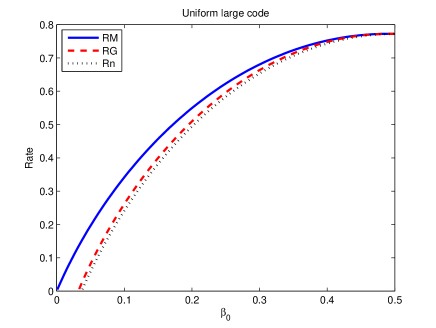
Figure 8: BNSC: matched and the mismatched decoder versus $q^{\star}$, for $\gamma_{0}=0.025$ , $\gamma_{1}=0.05$ and $p=0.5$.

Let the hamming power constraint be the same as for the BSC channel (143). Fig. 8 shows the achievable rates for the matched and mismatched decoders for $\gamma_{0}=0.025$ and $\gamma_{1}=0.05$. The matched decoder outperforms the mismatched as expected. At $\beta_{0}=0.5$, the typical codewords are transmitted since the large codebook is uniform, thus the two decoders are the same. The naive approach describes the performance of the typical codewords. In this case, the mismatched performs better than the naive approach, thus the non-typical codewords have lower average probability of error than the typical codewords.

VI-B Non-uniform large codebook

The non-uniform large codebook is the more general case. Although it is not common to use non-uniform distributions in practical system, we present several toy examples for the sake of completeness. The first example is the BNSC which satisfies the general condition (106) (required for the MJT bound to be valid). Otherwise, we can not compare all the bounds. The second example is generating a Gaussian codebook with power $\beta_{0}$ from a larger Gaussian codebook with average power $B_{0}$, where $\beta_{0}\ll B_{0}$.

VI-B1 BNSC

In this section we consider the binary non-symmetric channel, such that the general condition (106) is satisfied. In order to be able to demonstrate all our bounds (i.e., satisfy (106)) we have to choose a large codebook which is not uniformly distributed. In particular, the large codebook is according to $p\left(x\right)$ which solves

$$\left\{\begin{array}[]{c}\log p\left(x=0\right)-H\left(\gamma_{0}\right)=\log p\left(x=1\right)-H\left(\gamma_{1}\right),\\ p\left(x=0\right)+p\left(x=1\right)=1,\end{array}\right.$$ (152)

i.e.,

$$p\left(x=0\right)=\frac{\exp\left(H\left(\gamma_{0}\right)-H\left(\gamma_{1}\right)\right)}{\exp\left(H\left(\gamma_{0}\right)-H\left(\gamma_{1}\right)\right)+1}.$$ (153)

The hamming power constraint is used once again, limiting the average number of ones in a codeword to be lower than in the large codebook, i.e. $\beta_{0}\leq p\left(x=1\right)$.

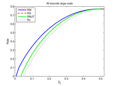
Figure 9: BNSC: matched and the mismatched decoder versus $\beta_{0}$, for $\gamma_{0}=0.025$ , $\gamma_{1}=0.05$ and $p=0.47$.

Fig. 9 shows the achievable rates for $\gamma_{0}=0.025$ and $\gamma_{1}=0.05$, using the matched and the mismatched decoders. The probability mass function of the large codebook (according to (153)) is $p=0.47$. In this example, the Gallager and the MJT are also above the naive approach. Furthermore, the Gallager and the MJT bounds are very close to each other. All bounds coincide at $q^{\star}=0.47$, since the typical codewords are transmitted.

VI-B2 Gaussian large code

In the following example we consider the situation where the large codebook has $2^{NR}$ codewords with average power $B_{0}$, according to Gaussian distribution. Whereas, the transmitted codewords have much smaller power $\beta_{0}\ll B_{0}$. It is easy to show that the conditional distribution in this case is also Gaussian with average power $\beta_{0}$. Thus, the capacity of the Gaussian channel is achieved for the matched decoder.

The mismatched decoder derivation is less trivial. Let us first derive the Gallager bound using

$$D\left(q^{\star}\left(X\right)\parallel p\left(X\right)\right)=$$

$$\frac{1}{2}\left(\frac{\beta_{0}}{B_{0}}-\log\frac{\beta_{0}}{B_{0}}-1\right),$$ (154)

where $q^{\star}\left(X\right)$ is Gaussian with variance $\beta_{0}$ and zero mean, and $p\left(X\right)$ is Gaussian with variance $B_{0}$ and zero mean. In a similar manner,

$$D\left(q^{\star}\left(Y\right)\parallel p\left(Y\right)\right)=$$

$$\frac{1}{2}\left(\frac{\beta_{0}+\sigma_{Z}^{2}}{B_{0}+\sigma_{Z}^{2}}-\log\frac{\beta_{0}+\sigma_{Z}^{2}}{B_{0}+\sigma_{Z}^{2}}-1\right),$$ (155)

assuming that the channel is AWGN with variance $\sigma_{Z}^{2}$ and zero mean. In the scenario where $\beta_{0}\ll B_{0}$ and $\sigma_{Z}^{2}\ll B_{0}$, the Gallager bound is deduced to

$$R_{G} \approx \frac{1}{2}\log\left(1+\frac{\beta_{0}}{\sigma_{Z}^{2}}\right)+\frac{1}{2}\log\left(\frac{\beta_{0}}{\beta_{0}+\sigma_{Z}^{2}}\right)$$ (156)

$$= \frac{1}{2}\log\left(\beta_{0}/\sigma_{Z}^{2}\right).$$

This example is related to nested lattice shaping. The nested lattice scheme consists of fine lattice and coarse lattice. The fine lattice is the “large codebook” (having infinite number of codewords). This lattice represents all the cosets. The coarse lattice provides the shaping region, such that it bounds the coset representatives (the minimum power codewords in each coset), which construct the shaped codebook. A practical decoding scheme for nested lattices is lattice decoding, which is in fact very similar to the mismatched decoder described in this paper. The large Gaussian codebook can be viewed as a region in the infinite lattice, which is large enough such that decoding in that codebook is the same as decoding in infinite lattice for codewords transmitted from the small codebook. It is interesting though to compare our bound (156) to the performance of lattice decoding [16], and indeed the result is identical.

VII Conclusions

In this paper, we proposed a method to analyze practical shaping schemes, in which a shaped subcode is chosen from a larger code (in most cases uniformly distributed large codebook). The codewords in the shaped codebook satisfy as set of constraints. We provide a theoretical framework for such analysis, using random coding and a selection process subject to constraints. In particular, we have found the achievable rates of the matched and the mismatched decoders, where the last is unaware of the selection process at the transmitter. This decoder is suboptimal, but occasionally more practical since it does not have to repeat the selection process at the receiver. In general, we show that the large code performance does not dictate the subcode performance, and that the non-typical codewords require different analysis. Hence, we obtained two novel achievable bounds for the mismatched decoding using a modification on the Gallager and the Joint Typicality bounding techniques. We examine several special cases in detail. In the special case of BSC, however, the large code analysis is actually valid and can be justified using capacity achieving linear codes. For M-PAM over AWGN the loss due to mismatched decoding is not very significant. We show other examples where there is a larger difference between the matched and mismatched decoding.

To obtain $I_{q^{\star},p}\left(X,Y\right)$ in closed form, we calculate the derivative of $E_{0}\left(\rho,q^{\star},p\right)$ with respect to $\rho$. Let us define

$$a\left(\rho,y\right) = \sum_{x}q^{\star}\left(x\right)p\left(y\mid x\right)^{\frac{1}{1+\rho}},$$ (157)

$$b\left(\rho,y\right) = \sum_{x}p\left(x\right)p\left(y\mid x\right)^{\frac{1}{1+\rho}},$$ (158)

$$c\left(\rho,y\right) = b\left(\rho,y\right)^{\rho}$$ (159)

$$= \exp\left(\rho\log b\left(\rho,y\right)\right),$$

$$d\left(\rho\right) = \sum_{y}a\left(\rho,y\right)c\left(\rho,y\right).$$ (160)

Substituting (157)-(160) into (92)

$$E_{0}\left(\rho,q,p\right)=-\log d\left(\rho\right).$$ (161)

Differentiating with respect to $\rho$, yields

$$\frac{\partial E_{0}\left(\rho,q,p\right)}{\partial\rho}=-\frac{\partial}{\partial\rho}\log d\left(\rho\right)$$

$$= -\frac{\sum_{y}\frac{\partial a\left(\rho,y\right)}{\partial\rho}c\left(\rho,y\right)+\frac{\partial c\left(\rho,y\right)}{\partial\rho}a\left(\rho,y\right)}{d\left(\rho\right)},$$ (162)

such that

$$\frac{\partial a\left(\rho,y\right)}{\partial\rho}=\frac{-\sum_{x}q^{\star}\left(x\right)p\left(y\mid x\right)^{\frac{1}{1+\rho}}\log p\left(y\mid x\right)}{\left(1+\rho\right)^{2}}$$ (163)

$$\frac{\partial b\left(\rho,y\right)}{\partial\rho}=\frac{-\sum_{x}p\left(x\right)p\left(y\mid x\right)^{\frac{1}{1+\rho}}\log p\left(y\mid x\right)}{\left(1+\rho\right)^{2}}$$ (164)

$$\frac{\partial c\left(\rho,y\right)}{\partial\rho}=c\left(\rho,y\right)\left(\log b\left(\rho,y\right)+\rho\frac{\frac{\partial b\left(\rho,y\right)}{\partial\rho}}{b\left(\rho,y\right)}\right).$$ (165)

Finally, using these terms at $\rho=0$, yields

$$\frac{\partial E_{0}\left(\rho,q,p\right)}{\partial\rho}\mid_{\rho=0}=$$

$$\sum_{y}\sum_{x}q^{\star}\left(x,y\right)\log p\left(y\mid x\right)$$

$$-\sum_{y}q^{\star}\left(y\right)\log p\left(y\right).$$ (166)

Subsequently, using the definitions of entropy (3), conditional entropy (4), mutual information (5) and the Kullback-Leibler information divergence (6) we conclude that

$$I_{q^{\star},p}\left(X,Y\right)=I_{q^{\star}}\left(X,Y\right)+D\left(q^{\star}\left(Y\right)\parallel p\left(Y\right)\right).$$ (167)

This gives $I_{q^{\star},p}\left(X,Y\right)$ in closed form.

References

- [1] G. D. Forney, “Trellis shaping,” IEEE Trans. Inform. Theory, vol. 38, pp. 281–300, Mar. 1992.
- [2] J. H. Conway and N. J. A. Sloane, “Voronoi regions of lattices, second moments of polytops, and quantization,” IEEE Trans. Inform. Theory, vol. IT-28, pp. 211-226, Mar. 1982.
- [3] G. D. Forney, Jr., “Multidimensional constellation—Part II: Voronoi Constellations,” IEEE J. Select. Areas Commun., vol. 7, pp. 941-958, Aug. 1989
- [4] .R. J. Barron, B. Chen, and G. W. Wornell, “The duality between information embedding and source coding with side information and some applications,” IEEE Trans. Inform. Theory, vol. 49, pp. 1159-1180, May 2003.
- [5] R. Zamir, S. S. (Shitz), and U. Erez, “Nested linear/lattice codes for structured multiterminal binning,” IEEE Trans. Inform. Theory, vol. 48, pp. 1250-1276, June 2002.
- [6] M. J. Wainwright, E. Martinian: “Low-Density Graph Codes that are optimal for binning and coding with side information,” IEEE Trans. Inform. Theory, vol. 55, pp. 1061-1079, March 2009.
- [7] Q. Wang and C. He, “Practical dirty paper coding with nested binary LDGM-LDPC codes,” in IEEE ICC, June 2009.
- [8] N. Varnica, X. Ma, and A. Kavčic̀, “Capacity of power constrained memoryless AWGN channels with fixed input constellations,” IEEE Global Communications Conference, Taipei, Taiwan, 2002.
- [9] U. Wachsmann, R. Fischer, and J. Huber, “Multilevel codes: Theoretical concepts and practical design rules,” IEEE Trans. Inform. Theory, vol. 45, 1999.
- [10] T. Cover, J. Thomas, “Elements of Information Theory,” 1991.
- [11] R. G. Gallager, “Information Theory and Reliable Communication,” New York: Wiley, 1968.
- [12] C. E. Shannon, “A mathematical theory of communication,” Bell Syst. Tech. J., vol. 27, pp. 379–423 and pp. 623–656, July and Oct. 1948.
- [13] R. Fischer, U. Wachsmann, and J. Huber, “On the combination of multilevel coding and signal shaping,” ITG Conf. Source and Channel Coding, pp. 273–278, Mar. 1998.
- [14] G. Ungerboeck, “Channel coding with multilevel/phase signals,” IEEE Trans. Inform. Theory, vol. IT-28, pp. 55–67, Jan. 1982.
- [15] Z. Zhao, “Capacity analysis of free-space optical communication channels with multiple receiver apertures,” Aerospace Conference, Mar. 2011
- [16] R. Zamir, “Lattice Coding for Signals and Networks,” Cambridge University Press, 2014.