Collective modes in the anisotropic unitary Fermi gas
and the inclusion of a backflow term

Abstract

We study the collective modes of the confined unitary Fermi gas under anisotropic harmonic confinement as a function of the number of atoms. We use the equations of extended superfluid hydrodynamics, which take into account a dispersive von Weizsäcker-like term in the equaton of state. Finally, we discuss the inclusion of a backflow term in the extended superfluid Lagrangian and the effects of this anomalous term on sound waves and Beliaev damping of phonons.

I Introduction

In this paper we calculate the collective monopole and quadrupole modes of the unitary Fermi gas (characterized by an infinite s-wave scattering length) under axially-symmetric anisotropic harmonic confinement by using the extended Lagrangian density of superfluids which we proposed a few years ago flavio , to study the unitary Fermi gas flavio ; flavio2 ; flavio3 ; flavio4 ; flavio5 ; flavio6 ; flavio7 ; flavio8 . The internal energy density of our extended Lagrangian density contains a term proportional to the kinetic energy of a uniform non interacting gas of fermions, plus a gradient correction of the von-Weizsacker form $\lambda\hbar^{2}/(8m)(\nabla n/n)^{2}$ von . The inclusion of a gradient term has been adopted for studying the quantum hydrodynamics of electrons by March and Tosi tosi , and by Zaremba and Tso tso . In the context of the BCS-BEC crossover, the gradient term is quite standard nick ; kim ; v2 ; v3 ; v4 ; v5 ; v6 ; v7 ; v8 . In the last part of this paper we consider the inclusion of backflow terms less ; treiner in the extended superfluid Lagrangian. By using our equations of extended superfluid hydrodynamics with backflow we calculate sound waves, static response function and structure factor of a generic uniform superfluid and also the effect of the backflow on Beliaev damping of phonons beliaev .

II Extended superfluid Lagrangian and hydrodynamic equations

The extended Lagrangian density of dilute and ultracold superfluids is given by flavio ; flavio2 ; flavio3 ; flavio4 ; flavio5 ; flavio6 ; flavio7 ; flavio8

$$\mathscr{L}=\mathscr{L}_{0}+\mathscr{L}_{W}$$ (1)

where

$$\mathscr{L}_{0}=-\hbar\,{\dot{\theta}}\,n-{\hbar^{2}\over 2m}({\boldsymbol{\nabla}}\theta)^{2}\,n-U({\bf r})\,n-{\cal E}_{0}(n)$$ (2)

is the familiar Popov’s Lagrangian density popov of superfluid hydrodynamics, with $n({\bf r},t)$ the local density and $\theta({\bf r},t)$ half of the phase of the condensate order parameter of Cooper pairs for superfluid fermions (or the phase of the condensate order parameter for superfluid bosons). Here $U({\bf r})$ is the external potential acting on particles and ${\cal E}_{0}(n)$ is the bulk internal energy of the system. The generalization of the superfluid hydrodynamics is due to the the Lagrangian density

$$\mathscr{L}_{W}=-\lambda{\hbar^{2}\over 8m}{({\boldsymbol{\nabla}}n)^{2}\over n}\;,$$ (3)

which takes into account density variations. Thus, the local internal energy depends not only on the local density $n({\bf r},t)$ but also on its space gradient, namely

$${\cal E}(n,{\boldsymbol{\nabla}}n)={\cal E}_{0}(n)+\lambda{\hbar^{2}\over 8m}{({\boldsymbol{\nabla}}n)^{2}\over n}\;,$$ (4)

where, as previously mentioned, ${\cal E}_{0}(n)$ is the internal energy of a uniform unitary Fermi gas with density $n$. The parameter $\lambda$ giving the gradient correction must be determined from microscopic calculations or from comparison with experimental data.

By using the Lagrangian density (1) the Euler-Lagrange equation for $\theta$ gives

$${\partial n\over\partial t}+{\hbar\over m}{\boldsymbol{\nabla}}\cdot\left(n\;{\boldsymbol{\nabla}}\theta\right)=0\;,$$ (5)

while the Euler-Lagrange equation for $n$ leads to

$$\hbar\,{\dot{\theta}}+{\hbar^{2}\over 2m}({\boldsymbol{\nabla}}\theta)^{2}+U({\bf r})+X(n,{\boldsymbol{\nabla}}n)=0\;,$$ (6)

where

$$X(n,{\boldsymbol{\nabla}}n)={\partial{\cal E}\over\partial n}-{\boldsymbol{\nabla}}\cdot{\partial{\cal E}\over\partial({\boldsymbol{\nabla}}n)}\;.$$ (7)

which describes how the internal energy varies as the local density and its gradient vary, may be considered a local chemical potential. The local velocity field ${\bf v}({\bf r},t)$ of the superfluid is related to $\theta({\bf r},t)$ by

$${\bf v}({\bf r},t)={\hbar\over m}{\boldsymbol{\nabla}}\theta({\bf r},t)\;.$$ (8)

This definition ensures that the velocity is irrotational, i.e. ${\boldsymbol{\nabla}}\wedge{\bf v}={\bf 0}$. By using the definition (8) in both Eqs. (5) and (6) and applying the gradient operator $\boldsymbol{\nabla}$ to Eq. (6) one finds the extended hydrodynamic equations of superfluids

$${\partial n\over\partial t}+{\boldsymbol{\nabla}}\cdot\left(n\;{\bf v}\right)=0\;.$$ (9)

$$m{\partial{\bf v}\over\partial t}+{\boldsymbol{\nabla}}\left[{1\over 2}m{\bf v}^{2}+U({\bf r})+X(n,{\boldsymbol{\nabla}}n)\right]={\bf 0}\;.$$ (10)

We stress that in the presence of an external confinement $U({\bf r})$ the chemical potential $\mu$ of the system does not coincide with the local chemical potential $X(n,{\boldsymbol{\nabla}}n)$. In the presence of an external potential the relation between the equilibrium (ground state) density $n_{0}({\bf r})$ and the chemical potential $\mu$ can be obtained from Eq. (6) by setting $\theta({\bf r},t)=-\mu t/\hbar$ and ${\bf v}({\bf r},t)={\bf 0}$, so that

$$U({\bf r})+X(n_{0},{\boldsymbol{\nabla}}n_{0})=\mu\;.$$ (11)

III Collective modes of the anisotropic unitary Fermi gas

In the case of the unitary Fermi gas the bulk internal energy can be written as

$${\cal E}_{0}(n)=\xi\,{3\over 5}{\hbar^{2}\over 2m}(3\pi^{2})^{2/3}\,n^{5/3}\;,$$ (12)

where $\xi\simeq 0.4$ is a universal parameter flavio ; flavio2 ; v4 ; son ; valle . and various approaches flavio ; flavio2 ; v4 ; v7 ; son ; valle suggest that $\lambda\simeq 0.25$. The local chemical potential is then:

$$X(n,{\boldsymbol{\nabla}}n)={\hbar^{2}\over 2m}(3\pi^{2})^{2/3}\xi\,n^{2/3}-\lambda{\hbar^{2}\over 2m}{\nabla^{2}\sqrt{n}\over\sqrt{n}}\;.$$ (13)

with the above mentioned values of $\xi$ and $\lambda$.

In this section we consider the unitary Fermi gas under the anisotropic axially-symmetric harmonic confinement

$$U({\bf r})=\frac{m}{2}\omega^{2}_{\rho}(x^{2}+y^{2})+\frac{m}{2}\omega_{z}^{2}z^{2}\;,$$ (14)

where $\omega_{\rho}$ is the cylindric radial frequency while $\omega_{z}$ is the axial frequency. In this case, Eq. (11) for the ground-state density profile $n_{0}({\bf r})$ becomes

$$\frac{m}{2}\omega^{2}_{\rho}(x^{2}+y^{2}) + \frac{m}{2}\omega_{z}^{2}z^{2}+{\hbar^{2}\over 2m}(3\pi^{2})^{2/3}\xi\,n_{0}(x,y,z)^{2/3}$$ (15)

$$- \lambda{\hbar^{2}\over 2m}{\nabla^{2}\sqrt{n_{0}(x,y,z)}\over\sqrt{n_{0}(x,y,z)}}=\mu\;.$$

We have solved numerically this 3D partial differential equation, by using a finite-difference predictor-corrector Crank-Nicholson method sala-numerics with imaginary time after chosing $\xi=0.42$ and $\lambda=0.25$. In the case of isotropic trap ($\omega_{\rho}/\omega_{z}=1$) the fermionic cloud is spherically symmetric and consequently axial and radial density profiles coincide. Instead, as expected, by increasing the trap anisotropy also the fermionic cloud becomes more anisotropic.

We are interested in calculating the frequencies of low-lying collective oscillations of the anisotropic unitary Fermi gas. Exact scaling solutions for the unitary Fermi gas have been considered by Castin castin and also by Hou, Pitaevskii, and Stringari forzati . Unfortunately, in the presence of anisotropic trapping potential and including the gradient term in the hydrodynamic equations, these scaling solutions are no more exact.

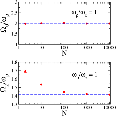
Figure 1: (Color online). Unitary Fermi gas under isotropic ($\omega_{\rho}=\omega_{z}$) harmonic confinement. In the two panels there are the monopole frequency $\Omega_{0}$ (upper panel) and the quadrupole frequency $\Omega_{2}$ (lower panel) as a function of the number $N$ of atoms. Filled circles with error bars: numerical results obtained solving Eqs. (9) and (10) with Eq. (13) and $\lambda=0.25$. Dashed lines: analytical results, i.e. exact Eq. (16) and Thomas-Fermi Eq. (17). Universal parameter of the unitary Fermi gas: $\xi=0.42$.

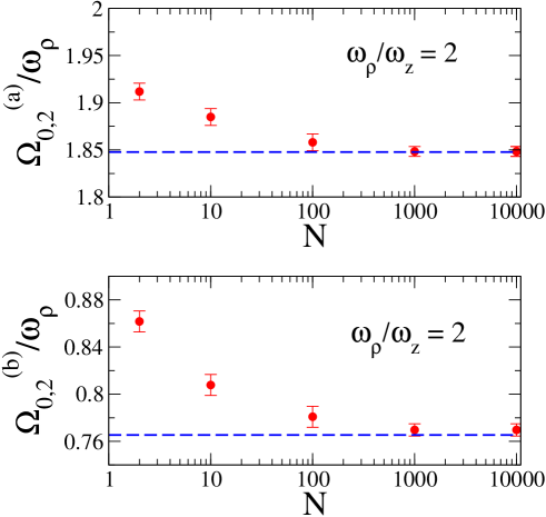
Figure 2: (Color online). Unitary Fermi gas under anisotropic but axially-symmetric ($\omega_{\rho}=2\omega_{z}$) harmonic confinement. In the two panels there are the two frequencies $\Omega_{0,2}^{(a)}$ and $\Omega_{0,2}^{(b)}$ of the coupled monopole and quadrupole modes as a function of the number $N$ of atoms. Filled circles with error bars: numerical results obtained solving Eqs. (9) and (10) with Eq. (13) and $\lambda=0.25$. Dashed lines: analytical results, i.e. Thomas-Fermi Eq. (18). Universal parameter of the unitary Fermi gas: $\xi=0.42$.

For this reason we solve numerically the extended hydrodynamic equations (9) and (10). In particular, by using our finite-difference predictor-corrector Crank-Nicolson code in real time sala-numerics , we integrate a time-dependent nonlinear Schrödinger equation, which is fully equivalent (see flavio ; flavio5 ) to Eqs. (9) and (10).

Fig. 1 refers to the unitary Fermi gas under isotropic ($\omega_{\rho}=\omega_{z}$) harmonic confinement. In the two panels we plot the monopole frequency $\Omega_{0}$ (upper panel) and the quadrupole frequency $\Omega_{2}$ (lower panel) as a function of the number $N$ of atoms. As expected castin , the frequency $\Omega_{0}$ of the monopole mode does not depend on the number $N$ of particles and it is given by

$$\Omega_{0}=2\omega_{\rho}\;.$$ (16)

On the contrary, the figure shows that the frequency $\Omega_{2}$ of the quadrupole mode depends on $N$ and for large values of $N$ it approaches asymptotically the value $\sqrt{2}\omega_{\rho}$, appropriate to the case of neglecting the gradient and backflow terms, see stringa . Note that the filled circles are the results with $\lambda=0.25$ while the dashed lines show the analytical results castin ; stringa . Remarkably, for small values of $N$ the gradient term enhances the quadrupole frequency $\Omega_{2}$. In the isotropic case ($\omega_{\rho}=\omega_{z}$) the quadrupole frequency $\Omega_{2}$ in the limit $N\to\infty$ it gives the Thomas-Fermi result (i.e. without the gradiente term) stringa

$$\Omega=\sqrt{2}\omega_{\rho}\;,$$ (17)

while in the limit $N\to 0$ it gives $\Omega=2\omega_{\rho}$, which is the quadrupole oscillation frequency of non-interacting atoms (the same result holds for ideal fermions and ideal bosons) lipparini .

In Figs. 2 we consider the unitary Fermi gas under anisotropic but axially-symmetric ($\omega_{\rho}=2\omega_{z}$) harmonic confinement. In this case monopole and quadrupole modes are coupled and we have determined numerically the two associated frequencies $\Omega_{0,2}^{(a)}$ and $\Omega_{0,2}^{(b)}$. Also in this case the gradient term increases the frequencies for small values of $N$. Moreover, for large values of $N$ these frequencies reduce to the results without gradient term stringa

$$\Omega_{0,2}^{(a),(b)}=\sqrt{\frac{5}{3}\omega_{\rho}^{2}+{4\over 3}\omega_{z}^{2}\pm{1\over 3}\sqrt{25\omega_{\rho}^{4}+16\omega_{z}^{4}-32\omega_{\rho}^{2}\omega_{z}^{2}}}\;,$$ (18)

which correspond to the dashed lines. Our calculations show that the frequency $\Omega_{2}$ of Fig. 2, and the frequencies $\Omega_{0,2}^{(a)}$ and $\Omega_{0,2}^{(b)}$ of Figs. 2 give a clear signature of the presence of the von-Weizsacker gradient term.

We stress that current experiments with ultracold atoms at unitarity can detect deviations from the Thomas-Fermi approximation, as done some years ago for Bose-Einstein condensates jin .

IV Inclusion of a backflow term

Inspired by the papers of Son and Wingate son and Manes and Valle valle in this section we consider the inclusion of a backflow term in the extended superfluid Lagrangian. This backflow term depends on the velocity strain, as suggested for superfluid ⁴He many years ago by Thouless less and more recently by Dalfovo and collaborators treiner . In particular, we consider the Lagrangian density

$$\mathscr{L}=\mathscr{L}_{0}+\mathscr{L}_{W}+\mathscr{L}_{B}\;,$$ (19)

where $\mathscr{L}_{0}$ and $\mathscr{L}_{W}$ are given by Eqs. (2) and (3) respectively, and the backflow term $\mathscr{L}_{B}$ reads

$$\mathscr{L}_{B}=-{\hbar^{2}\over m}n^{1/3}[\gamma_{1}(\nabla^{2}\theta)^{2}+\gamma_{2}(\partial_{i}\partial_{j}\theta)^{2}]\;.$$ (20)

Notice that $i,j=x,y,z$ and summations over repeated indices are implied. Again, for a generic superfluid the parameters $\gamma_{1}$ and $\gamma_{2}$ of the backflow term must be determined from microscopic calculations or from comparison with experimental data.

The Lagrangian density (19) depends on the dynamical variables $\theta({\bf r},t)$ and $n({\bf r},t)$. The conjugate momenta of these dynamical variables are then given by

$$\pi_{\theta} = {\partial\mathscr{L}\over\partial{\dot{\theta}}}=-\hbar\,n\;,$$ (21)

$$\pi_{n} = {\partial\mathscr{L}\over\partial{\dot{n}}}=0\;,$$ (22)

and the corresponding Hamiltonian density reads

$$\mathscr{H}=\pi_{\theta}\,{\dot{\theta}}+\pi_{n}\,{\dot{n}}-\mathscr{L}=-\hbar\,n\,{\dot{\theta}}-\mathscr{L}\;,$$ (23)

namely

$$\mathscr{H} = {\hbar^{2}\over 2m}({\boldsymbol{\nabla}}\theta)^{2}\,n+U({\bf r})\,n+{\cal E}_{0}(n)$$

$$+ \lambda{\hbar^{2}\over 8m}{({\boldsymbol{\nabla}}n)^{2}\over n}+{\hbar^{2}\over m}n^{1/3}[\gamma_{1}(\nabla^{2}\theta)^{2}+\gamma_{2}(\partial_{i}\partial_{j}\theta)^{2}]\;,$$

which is the sum of the flow kinetic energy density $\hbar^{2}({\boldsymbol{\nabla}}\theta)^{2}n/(2m)=(1/2)mv^{2}n$, the external energy density $U({\bf r})n$, the internal energy density ${\cal E}_{0}(n)$ without the gradient correction, the gradient correction $\lambda({\hbar^{2}/8m}){({\boldsymbol{\nabla}}n)^{2}/n}$ to the internal energy, and the backflow energy density $({\hbar^{2}/m})n^{1/3}[\gamma_{1}(\nabla^{2}\theta)^{2}+\gamma_{2}(\partial_{i}\partial_{j}\theta)^{2}]=mn^{1/3}[\gamma_{1}({\boldsymbol{\nabla}}\cdot{\bf v})^{2}+\gamma_{2}(\partial_{i}v_{j})^{2}]$.

The Hamiltonian density (IV) is nothing else than the energy density recently found by Manes and Valle valle with a derivative expansion from their effective field theory of the the Goldstone field son ; valle . The effective field theory of Manes and Valle valle traces back to the old hydrodynamic results of Popov popov and generalizes the one derived by Son and Wingate son for the unitary Fermi gas from general coordinate invariance and conformal invariance. Actually, at next-to-leading order Son and Wingate son found an additional term proportional to $\nabla^{2}U({\bf r})$, which has been questioned by Manes and Valle valle and which is absent in our approach. In addition, Manes and Valle valle have stressed that the conformal invariance displayed by the unitary Fermi gas implies

$$\gamma_{2}=-3\gamma_{1}\;.$$ (25)

Note that a paper of Schakel schakel confirms the results of Manes and Valle.

We are interested on the propagation of sound waves in superfluids. For simplicity we set $U({\bf r})=0$, and consider a small fluctuation $\phi({\bf r},t)$ of the phase $\theta({\bf r},t)$ around the stationary phase $\theta_{0}(t)=-({\mu/\hbar})t$, namely

$$\phi({\bf r},t)=\theta({\bf r},t)-\theta_{0}(t)\;,$$ (26)

and a small fluctuation ${\rho}({\bf r},t)$ of the density $n({\bf r},t)$ around the constant and uniform density $n_{0}$, namely

$${\rho}({\bf r},t)=n({\bf r},t)-n_{0}\;.$$ (27)

From the full Lagrangian density (19) it is then quite easy to find the quadratic Lagrangian density $\mathscr{L}^{(2)}$ of the fluctuating fields $\phi({\bf r},t)$ and $\rho({\bf r},t)$:

$$\mathscr{L}^{(2)} = -\hbar\,{\dot{\phi}}\,\rho-{\hbar^{2}n_{0}\over 2m}({\boldsymbol{\nabla}}\phi)^{2}-{mc_{s}^{2}\over 2n_{0}}\rho^{2}$$

$$- \lambda{\hbar^{2}\over 8m\,n_{0}}({\boldsymbol{\nabla}}\rho)^{2}-\gamma{\hbar^{2}n_{0}^{1/3}\over m}(\nabla^{2}\phi)^{2}\;,$$

where $c_{s}$ is the sound velocity of the generic superfluid, given by

$$c_{s}^{2}={n_{0}\over m}{\partial^{2}{\cal E}_{0}(n_{0})\over\partial n^{2}}\;,$$ (29)

and $\gamma=\gamma_{1}+\gamma_{2}$. In fact, $(\nabla^{2}\theta)^{2}$ and $(\partial_{i}\partial_{j}\theta)^{2}$ differ by a total derivative valle and consequently, since at the quadratic order the coefficients in front of them are constants, one derives Eq. (IV) with $\gamma=\gamma_{1}+\gamma_{2}$. The linear equations of motion associated to the quadratic Lagrangian $\mathscr{L}_{2}$ read

$${\partial\over\partial t}\rho+n_{0}{\boldsymbol{\nabla}}\cdot{\bf v}-{2}n_{0}^{1/3}\gamma\,\nabla^{2}({\boldsymbol{\nabla}}\cdot{\bf v})=0\;,$$ (30)

$${\partial\over\partial t}{\bf v}+{c_{s}^{2}\over n_{0}}{\boldsymbol{\nabla}}\rho-{\lambda\hbar^{2}\over 4m^{2}n_{0}}{\boldsymbol{\nabla}}(\nabla^{2}\rho)=0\;,$$ (31)

with ${\bf v}=(\hbar/m)\nabla\phi$. These equations can be arranged in the form of the following wave equation

$$\Big{[}{\partial^{2}\over\partial t^{2}}-c_{s}^{2}\nabla^{2} + \Big{(}\lambda{\hbar^{2}\over 4m^{2}}+\gamma{2c_{s}^{2}\over n_{0}^{2/3}}\Big{)}\nabla^{4}$$

$$- \lambda\gamma{\hbar^{2}\over 2m^{2}n_{0}^{2/3}}\nabla^{6}\Big{]}\rho({\bf r},t)=0\;.$$

This wave equation admits monochromatic plane-wave solutions, where the frequency $\omega$ and the wave vector ${\bf q}$ are related by the dispersion formula $\omega=\omega(q)$ given by

$$\hbar\,\omega(q)=\sqrt{\Big{(}{\hbar^{2}q^{2}\over 2m}+\gamma{\hbar^{2}q^{4}\over mn_{0}^{2/3}}\Big{)}\Big{(}\lambda{\hbar^{2}q^{2}\over 2m}+2mc_{s}^{2}\Big{)}}\;.$$ (33)

Notice that a negative value of $\gamma$ implies that the frequency $\omega(q)$ becomes imaginary for $q>n_{0}^{1/3}/\sqrt{2|\gamma|}$. However, $\gamma$ is expected to be very small and the hydrodynamics is no loger valid for these large values of $q$.

It is instead useful to expand $\omega(q)$ for small values of $q$ (long-wavelength hydrodynamic regime), finding

$$\hbar\,\omega(q)=c_{s}\,\hbar q+{\hbar\over 2}\big{(}\lambda{\hbar^{2}\over 4m^{2}c_{s}}+\gamma{2c_{s}\over n_{0}^{2/3}}\big{)}\,q^{3}+...\;.$$ (34)

The dispersion relation is linear in $q$ only for small values of the wavenumber $q$ and the coefficient of cubic correction depends on a combination of the gradient parameter $\lambda$ and backflow parameter $\gamma$. For $\gamma=0$ one recovers the dispersion relation we have proposed some years ago flavio , while setting also $\lambda=0$ one gets the familiar linear dispersion relation $\omega=c_{s}\,q$ of phonons. In the case of the unitary Fermi gas one has

$$c_{s}^{2}={\hbar^{2}\over m^{2}}{\xi\over 3}(3\pi^{2})^{2/3}n_{0}^{2/3}\;.$$ (35)

Moreover, we have seen that the backflow parameters are related by the formula (25), which means

$$\gamma=\gamma_{1}+\gamma_{2}=-2\gamma_{1}\;.$$ (36)

Consequently, at the cubic order in $q$ Eq. (33) gives

$${\omega(q)\over c_{s}k_{F}}={q\over k_{F}}+\Gamma\,{q^{3}\over k_{F}^{3}}\;,$$ (37)

where $k_{F}=(3\pi^{2}n_{0})^{2/3}$ is the Fermi wavenumber and

$$\Gamma={3\lambda\over 8\xi}-2(3\pi^{2})^{2/3}\gamma_{1}\;.$$ (38)

Within a mean-field approximation Manes and Valle valle have found $\gamma_{1}\simeq 0.006$, which implies $\gamma\simeq-0.012$ and $\Gamma\simeq 0.12$, using $\xi=0.4$ and $\lambda=0.25$. As recently discussed by Mannarelli, Manuel and Tolos tolos , the sign of $\Gamma$ has a dramatic effect on the possible phonon interaction channels: the three-phonon Beliaev process, i.e. the decay of a phonon into two phonons beliaev , is allowed only for positive values of $\Gamma$. Under this condition ($\Gamma\geq 0$) the phonon has a finite life-time and the frequency $\omega(q)$ possesses an imaginary part $\mbox{Im}[{\omega(q)}]$ due to this three-phonon decay beliaev ; lev . In particular, we find

$$\mbox{Im}[{\omega(q)}]=-{\hbar q^{5}\over 270\,\pi\,m\,n_{0}}\;.$$ (39)

This formula of Beliaev damping is easily derived from Beliaev theory beliaev ; lev taking into account Eq. (35).

It is important to point out that the sign of $\Gamma$ in Eq. (37) was debated also without the backflow term. In 1998 Marini, Pistolesi and Strinati marini found $\Gamma>0$ at unitarity by including Gaussian fluctuations to the mean-field BCS-BEC crossover. In 2005 Combescot, Kagan and Stringari combescot derived Eq. (37) with a negative $\Gamma$ at unitarity on the basis of a dynamical BCS model. In 2011 Schakel schakel obtained a positive $\Gamma$ at unitarity by using a derivative expansion technique, finding exactly the values of $\Gamma$ predicted by Ref. marini in the full BCS-BEC crossover.

To conclude this section, we observe that, for a generic many-body system, the dispersion relation can be written as lipparini

$$\hbar\,\omega(q)=\sqrt{m_{1}(q)\over m_{-1}(q)}\;,$$ (40)

where $m_{n}(q)$ is the $n$ moment of the dynamic structure function $S(q,\omega)$ of the many-body system under investigation, namely lipparini

$$m_{n}(q)=\int_{0}^{\infty}d\omega\ S(q,\omega)\ (\hbar\omega)^{n}\;.$$ (41)

In our problem, Eq. (IV), it is straightforward to recognize (see also treiner ) that

$$m_{1}(q)={\hbar^{2}q^{2}\over 2m}+\gamma{\hbar^{2}q^{4}\over mn_{0}^{2/3}}$$ (42)

and

$$m_{-1}(q)={1\over\lambda{\hbar^{2}q^{2}\over 2m}+2mc_{s}^{2}}\;.$$ (43)

In general, the static response function $\chi(q)$ is defined as lipparini

$$\chi(q)=-2\ m_{-1}(q)\;;$$ (44)

in our problem it reads:

$$\chi(q)=-{2\over\lambda{\hbar^{2}q^{2}\over 2m}+2mc_{s}^{2}}\;,$$ (45)

which satisfies the exact sum rule $\chi(0)=-1/mc_{s}^{2}$ lipparini . The static structure factor $S(q)$, defined as lipparini

$$S(q)=m_{0}(q)=\int_{0}^{\infty}d\omega\ S(q,\omega)\;,$$ (46)

can be approximated by the expression

$$S(q)=\sqrt{m_{1}(q)\,m_{-1}(q)}=\sqrt{{\hbar^{2}q^{2}\over 2m}+\gamma{\hbar^{2}q^{4}\over mn_{0}^{2/3}}\over\lambda{\hbar^{2}q^{2}\over 2m}+2mc_{s}^{2}}\;,$$ (47)

which gives an upper bound of $S(q)$ lipparini and reduces to $S(q)=\hbar q/(2mc_{s})$ for small $q$.

Finally, we remark that one can also calculate the frequencies $\Omega$ of collective oscillations of the unitary Fermi gas under the action of the trapping potential given by Eq. (14) taking into account the backflow. We have verified that in the case of spherically-symmetric harmonic confinement ($\omega_{\rho}=\omega_{z}$) the monopole mode $\Omega_{0}$ is not affected by the backflow term, i.e. $\Omega_{0}=2\omega_{\rho}$. Moreover, for large values of $N$ the contribution due to the backflow becomes negligible, similarly to the von Weizsäcker one.

V Conclusions

We have calculated collective modes of the anisotropic unitary Fermi gas by using the equations of extended superfluid hydrodynamics. In particular, we have shown that a gradient correction of the von-Weizsacker form in the hydrodynamic equations strongly affects the frequencies of collective modes of the system under axially-symmetric anisotropic harmonic confinement. We have found that, for both monopole and quadrupole modes, this effect becomes negligible only in the regime of a large number of fermions, where one recovers the predictions of superfluid hydrodynamics stringa . In the last part of the paper we have considered the inclusion of a backflow term in the extended hydrodynamics of superfluids.

We believe our results can trigger the interest of experimentalists. Some years ago beyond-Thomas-Fermi effects due to the dispersive gradient term have been observed by measuring the frequencies of collective modes in trapped Bose-Einstein condensates jin . Moreover, the spectrum of phonon excitations and Beliaev decay have been observed in a quasi-uniform Bose-Einstein condensate with Bragg pulses nir . Performing similar measurements in the unitary Fermi gas can shed light on the role played by gradient and backflow corrections in the superfluid hydrodynamics.

References

- (1) L. Salasnich and F. Toigo, Phys. Rev. A 78, 053626 (2008).
- (2) L. Salasnich, Laser Phys. 19, 642 (2009).
- (3) F. Ancilotto, L. Salasnich, and F. Toigo, Phys. Rev. A 79, 033627 (2009).
- (4) S.K. Adhikari and L. Salasnich, New J. Phys. 11, 023011 (2009).
- (5) L. Salasnich, F. Ancilotto, and F. Toigo, Laser Phys. Lett. 7, 78 (2010).
- (6) L. Salasnich, EPL 96, 40007 (2011).
- (7) F. Ancilotto, L. Salasnich, and F. Toigo, Phys. Rev. A 85, 063612 (2012).
- (8) L. Salasnich, Few-Body Syst. 54, 697 (2013).
- (9) C.F. von Weizsäcker, Zeit. Phys. 96, 431 (1935).
- (10) N.H. March and M. P. Tosi, Proc. R. Soc. A 330, 373 (1972).
- (11) E. Zaremba and H.C. Tso, Phys. Rev. B 49, 8147 (1994).
- (12) N. Manini and L. Salasnich, Phys. Rev. A, 71, 033625 (2005); G. Diana, N. Manini, and L. Salasnich, Phys. Rev. A, 73, 065601 (2006).
- (13) Y.E. Kim and A.L. Zubarev, Phys. Rev. A 70, 033612 (2004).
- (14) M.A. Escobedo, M. Mannarelli and C. Manuel, Phys. Rev. A 79, 063623 (2009).
- (15) E. Lundh and A. Cetoli, Phys. Rev. A 80, 023610 (2009).
- (16) G. Rupak and T. Schäfer, Nucl. Phys. A 816, 52 (2009).
- (17) S.K. Adhikari, Laser Phys. Lett. 6, 901 (2009).
- (18) W.Y. Zhang, L. Zhou, and Y.L. Ma, EPL 88, 40001 (2009).
- (19) A. Csordas, O. Almasy, and P. Szepfalusy, Phys. Rev. A 82, 063609 (2010).
- (20) S. N. Klimin, J. Tempere, and J.P.A. Devreese, J. Low Temp. Phys. 165, 261 (2011).
- (21) D.J. Thouless, Ann. Phys. 52, 403 (1969).
- (22) F. Dalfovo, A. Lastri, L. Pricaupenko, S. Stringari, and J. Treiner, Phys. Rev. B 52, 1193 (1995).
- (23) S.T. Beliaev, Sov. Phys. JETP 7, 299 (1958).
- (24) V.N. Popov, Functional Integrals in Quantum Field Theory and Statistical Physics (Reidel, Dordrecht, 1983).
- (25) E. Cerboneschi, R. Mannella, E. Arimondo, and L. Salasnich, Phys. Lett. A 249, 495 (1998); G. Mazzarella and L. Salasnich, Phys. Lett. A 373, 4434 (2009).
- (26) Y. Castin, Comptes Rendus Physique 5, 407 (2004).
- (27) Y.-H. Hou, L.P. Pitaevskii, and S. Stringari, Phys. Rev. A. 87, 033620 (2013).
- (28) M Cozzini, S. Stringari, Phys. Rev. Lett. 91, 070401 (2003).
- (29) D.S. Jin, J. R. Ensher, M. R. Matthews, C. E. Wieman, and E. A. Cornell, Phys. Rev. Lett. 77, 420 (1996).
- (30) D.T. Son and M. Wingate, Ann. Phys. (N.Y.) 321, 197 (2006).
- (31) J.L. Manes and M.A. Valle, Ann. Phys. (N.Y.) 324, 1136 (2009).
- (32) A.M.J. Schakel, Ann. Phys. (N.Y.) 326, 193 (2011).
- (33) M. Mannarelli, C. Manuel, and L. Tolos, e-preprint arXiv:12.5152.
- (34) L.P. Pitaevskii and S. Stringari, Bose-Einstein Condensation (Oxford Univ. Press, Oxford, 2003), pp. 72-74.
- (35) E. Lipparini, Modern Many-Particle Physics: Atomic Gases, Nanostructures and Quantum Liquids (World Scientific, Singapore, 2008).
- (36) M. Marini, F. Pistolesi, and G.C. Strinati, Eur. Phys. J B 1, 151 (1998).
- (37) R. Combescot, M.Yu. Kagan, and S. Stringari, Phys. Rev. A 74, 042717 (2006).
- (38) E.E. Rowen, N. Bar-Gill, and N. Davidson, Phys. Rev. Lett. 101, 010404 (2008); E.E. Rowen, N. Bar-Gill, R. Pugatch, and N. Davidson, Phys. Rev, A 77, 033602 (2008).