Systematic study of magnetic linear dichroism and birefringence in (Ga,Mn)As

Abstract

Magnetic linear dichroism and birefringence in (Ga,Mn)As epitaxial layers is investigated by measuring the polarization plane rotation of reflected linearly polarized light when magnetization lies in the plane of the sample. We report on the spectral dependence of the rotation and ellipticity angles in a broad energy range of $0.12-2.7\ \mathrm{eV}$ for a series of optimized samples covering a wide range on Mn-dopings and Curie temperatures and find a clear blue shift of the dominant peak at energy exceeding the host material band gap. These results are discussed in the general context of the GaAs host band structure and also within the framework of the $k\cdot p$ and mean-field kinetic-exchange model of the (Ga,Mn)As band structure. We find a semi-quantitative agreement between experiment and theory and discuss the role of disorder-induced non-direct transitions on magneto-optical properties of (Ga,Mn)As.

I Introduction

Among optical spectroscopies, differential methods based on the birefringence or the dichroism, i.e., sensitive to differences in refractive indices between two optical modes, can give more information on material electronic structure than absorption measurements.Ferre and Gehring (1984) For instance, the absorption coefficient $\alpha(\omega)$ in the dilute magnetic semiconductorJungwirth et al. (2006a) (DMS) (Ga,Mn)As is essentially featurelessBurch et al. (2004) at frequencies $\omega$ close to $E_{g}/\hbar$ (the band gap energy, $E_{g}\approx 1.52\ \mathrm{eV}$ for GaAs) while the same material in the same frequency range exhibits a strong peak in polarization plane rotation caused by the magnetic linear dichroism and birefringence.Kimel et al. (2005) At the same time, any type of magnetism-induced dichroism or birefringence depends on the ferromagnetic splitting of the bands (related to saturated magnetization $\vec{M}$) and manganese-doped DMSs like (Ga,Mn)As offer the unique possibility of tuning the strength of magnetism by varying the Mn content $x_{\mathrm{nom}}$ over a broad range. Studying the trends in magneto-optical spectra across a series of samples with increasing Mn doping and comparing them to model calculations allows to microscopically relate the individual spectral features to the electronic structure of the (Ga,Mn)As material.

Polarization-resolved magneto-optical effects appear in a multitude of geometries and setups which we review in more detail in Sec. II below. In terms of the leading order of the effect, they can be divided into effects linear and quadratic in $\vec{M}$. In both cases, an incident light beam linearly polarized along $\hat{x}^{\prime}$ turns into an elliptically polarized one whose major axis is rotated with respect to $\hat{x}^{\prime}$ by an angle $\theta$. The degree of ellipticity is characterized by another (typically also small) angle $\psi$. Both angles are defined in Fig. 1a. Effects linear (or more generally odd) in $\vec{M}$ give $\theta(-\vec{M})=-\theta(\vec{M})$ and are related,Kim et al. (2007); Acbas et al. (2009) for $\omega\to 0$, to the dc anomalous Hall effect.Nagaosa et al. (2010) These effects are more commonly investigated as they are often simpler to experimentally access. They are typically larger and it is simpler to separate them from magnetization-independent optical signals. On the other hand, even effects (quadratic in the leading order of $\vec{M}$) with $\theta(-\vec{M})=\theta(\vec{M})$ appear in literature less frequently. For example, the Voigt effect in reflection (see Sec. II and Fig. 2) has first been reported as late as in 1990.Schafer:1990_a Yet, they offer an alternative probe into the electronic structure of the material distinct from what is probed in odd-in-$\vec{M}$ measurements. The effects even in $\vec{M}$ are related to the anisotropic magnetoresistanceKokado et al. (2012); Rushforth et al. (2007) for $\omega\to 0$ and they do not vanish in certain situations where the effects odd in $\vec{M}$ do. For example in compensated antiferromagnets, the magneto-optical effects even in $\vec{M}$ can still be detected Kirilyuk et al. (2010) because contributions from the two spin-sublattices with opposite spin orientations do not cancel. As a probe into the antiferromagnetic order,Kimel et al. (2004) magneto-optical effect in the visible and infrared range, such as the one described in this article, does not rely on large-scale facilities as in the case of neutron diffraction or x-ray Voigt effect.Mertins et al. (2001)

The magneto-optical effects odd in $\vec{M}$ have been extensively explored in (Ga,Mn)As.Jungwirth et al. (2006a); Ando et al. (1998); Jungwirth et al. (2010); Acbas et al. (2009) While the visibleAndo et al. (1998); Jungwirth et al. (2010) range provides information on transitions between valence and conduction bands which are relatively less sensitive to the spin-orbit interaction effects, infra-redAcbas et al. (2009) spectra enable to explore transitions within valence bands. Quadratic (even in $\vec{M}$) magneto-optical response of (Ga,Mn)As is an alternative probe into its electronic structure. In analogy with the dc anisotropic magnetoresistance, it crucially depends on the spin-orbit interaction in the whole spectral range. Previous experiments have focused on measurements of the even in $\vec{M}$ magneto-optical effects in selected (Ga,Mn)As samples without studying their spectral dependenceMoore et al. (2003) or limiting themselves to the visible spectral range.Kimel et al. (2005); Tesařová et al. (2012) Here, we report measurements in a spectral range of 0.12 to 2.7 eV and study systematically the magneto-optical spectra even in $\vec{M}$ across a series of optimized (Ga,Mn)As materials spanning a broad Mn-doping range summarized in Tab. 1 below.

Section II is dedicated to a brief overview of magneto-optical effects and clarification of the terminology that is not coherent across the literature.Ferre and Gehring (1984); Kimel et al. (2005) Our experimental data are presented in Section III and we compare them in Section IV to a kinetic-exchange modelAbolfath et al. (2001)-based calculations of ac permittivity that allow us to determine $\theta(\omega)$ and $\psi(\omega)$. In Section IV, we also discuss the complex individual spectral features of $\theta(\omega)$ and clarify the role of linear birefringence and dichroism (see also Appendix D). Section V concludes the article. In Appendix A, we review theoretical description of magneto-optical effects on the level of Maxwell’s equations to which the permittivity tensor is the input. Appendices B, C and D, respectively contain additional experimental data, more details on the transport calculation using the kinetic-exchange model, and details on the optical part modelling, e.g. multiple reflections on the (Ga,Mn)As epilayer.

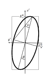
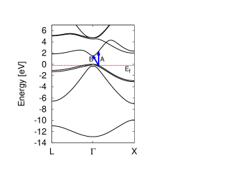
(a)	(b)

Figure 1: (a) Measured magneto-optical quantities. Originally linearly polarized beam becomes elliptically polarized after interaction with the sample. Its ellipticity is characterized by angle $\psi$ and rotation of the major axis is $\theta$. (b) GaAs host band structure with Fermi level $E_{f}$ typical for our Mn-doped samples. Arrows indicate direct (A) and non-direct (B) transitions from the Fermi surface to the conduction band.

II Overview of magneto-optical effects

The purpose of this section is to recapitulate selected magneto-optical effects, clarify the terminology and specify which of these effects is considered in this article. The first magneto-optical phenomenon was observed by Michael Faraday in 1846, followed by another one found by John Kerr in 1877. They found that linearly polarized light transmitted through (Faraday’s discovery) or reflected from (Kerr’s discovery) a non-magnetic material subject to magnetic field $\vec{B}$ has its polarization plane rotated. In their experiments, the wavevector of the propagating light $\vec{k}$ was parallel to $\vec{B}$. In 1899, Woldemar Voigt observed optical anisotropy of a non-magnetic crystal for $\vec{k}\perp\vec{B}$ which can also cause similar rotation of the polarization plane. Historical overview of these and related discoveries can be found in the introductory parts of Refs. Ebert, 1996; Ferre and Gehring, 1984. As a matter of definition, we will not include polarization-unrelated (or unresolved) effects such as cyclotron resonance into our further discussion.not (a)

Analogous phenomena are found in magnetic materials where, phenomenologically, $\vec{M}$ plays the same role as $\vec{B}$ in the original observations of Faraday, Kerr and Voigt. Typical experiments involve a slab or thin layer of the material and, for simplicity, let us assume for now that it is not placed on a substrate and also that $\vec{k}$ is perpendicular to the plane of the sample surface (”normal incidence”). Faraday and Kerr magneto-optical effects arise for $\vec{M}\parallel\vec{k}$, i.e., out-of-plane magnetization while Voigt effect occurs for in-plane magnetization ($\vec{M}\perp\vec{k}$). As it has already been described above (see Fig. 1a), the incident beam is linearly polarized and the Kerr (Faraday or Voigt) effect are manifested in the rotation $\theta$ of the reflected (transmitted) beam polarization plane. Any of these effects will, in general, be accompanied by a non-zero ellipticity characterized by $\psi$ and both angles are sometimes combined into one complex quantity, e.g. the complex Faraday angle $\theta_{F}$ in Ref. Kim et al., 2007. The Voigt effect is even in $\vec{M}$ while the Faraday and Kerr effects are odd in $\vec{M}$. There is no broadly accepted term for the quadratic (even-in-$\vec{M}$) magneto-optical effect in the reflection at normal incidence with in-plane $\vec{M}$, although sometimes it is called quadratic magneto-optical Kerr effect (QMOKE),Buchmeier et al. (2009) Hubert-Schäfer effectnot (b) or it is included in the ”reflection analogy to the Voigt effect”.Postava et al. (1997) We will adopt here the last terminology. A schematic summary of the Faraday, Voigt and Kerr effects and of the Voigt effect in reflection is shown in Fig. 2.

For other than the normal incidence, the Kerr effect is no longer distinguished by $\vec{M}\parallel\vec{k}$ and it appears in several variants. General magnetization $\vec{M}$ can now be decomposed into out-of-plane component $M_{\perp}$ and in-plane components $M_{L}$ ($M_{T}$) parallel (perpendicular) to the plane of incidence. The polar Kerr effect, sometimes also called magneto-optical Kerr effect (MOKE), is in the leading order linear in $M_{\perp}$ and it is the only effect odd in $\vec{M}$ that does not vanish for $M_{L}=M_{T}=0$. The longitudinal and transversal Kerr effects depend on the in-plane components of magnetization and to separate them from the Voigt effect in reflection, the polarization signal dependence on the angle $\beta$ between $\vec{M}$ and the polarization plane can be used. Unlike all three Kerr effects, Voigt effect in reflection is proportionalPostava et al. (1997) to a combination of $M_{T}^{2},M_{L}^{2}$ and $M_{L}M_{T}$ which, at normal incidence, combines into a $\sin 2\beta$ dependence.

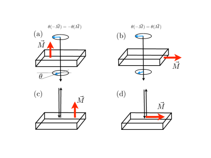
Figure 2: Selected magneto-optical effects. Polarization planes of incoming and outgoing beams are rotated by $\theta$ with respect to each other (possible ellipticity $\psi$ of the outgoing is not considered in these sketches). (a) Faraday effect, (b) Voigt effect, (c) Kerr effect, (d) Voigt effect in reflection.

In this work, we present a systematic spectral study of the Voigt effect in reflection. As with other magneto-optical phenomena, this effect includes rotation and ellipticity measured in the beam after its interaction with the sample and from now on, we associate the terms ”rotation” ($\theta$) and ”ellipticity” ($\psi$) only with the Voigt effect in reflection (unless explicitly stated otherwise). Both rotation and ellipticity are related to complex refractive indices $n_{\parallel}$ and $n_{\perp}$ of two modes (see detailed explanation in Appendix A) linearly polarized parallel and perpendicular to $\vec{M}$. Rotation $\theta$ is caused both by magnetic linear birefringence $\Delta\bar{n}\equiv\mbox{Re }(n_{\perp}-n_{\parallel})\not=0$ (MLB) and magnetic linear dichroism $\Delta\bar{k}\equiv\mbox{Im }(n_{\perp}-n_{\parallel})\not=0$ (MLD), an illustrative example is given in Appendix D. We now proceed to describe our experimental results of rotation and ellipticity of the Voigt effect in reflection on (Ga,Mn)As samples.

III Experiment

The samples used in our measurement are (Ga,Mn)As layers prepared by optimized molecular-beam epitaxy growth and post-growth annealing proceduresNemec et al. (2013) with various nominal Mn doping ranging from $x_{\mathrm{nom}}=1.5\%$ to 14% and cut into 4.5 by 5 mm chips. The basic material characteristics of our samples are listed in Tab. 1, additional information can be found in the main text and supplementary information of Refs. Jungwirth et al., 2010,Nemec et al., 2013. All samples were grown on a GaAs substrate, producing a compressive strain which favours an in-plane orientation of the easy axes (EAs). The competition of in-plane cubic and uniaxial anisotropies results in our (Ga,Mn)As films in two magnetic EAs tilted from the [100] and [010] crystal axes towards the $[1\bar{1}0]$ in-plane diagonal.Zemen et al. (2009) The tilt angle increasesNemec et al. (2013) with increasing Mn-doping. The sample substrates were wedged (1^∘) to avoid spurious signals that might appear due to the multiple reflections from the back side of the substrate. In order to measure the rotation and ellipticity angles $\theta$ and $\psi$ in a broad energy range we developed a sensitive experimental technique which is described in detail in Ref. Tesařová et al., 2012. We use a Xe lamp (0.33–2.7 eV) with a double prism CaF₂ monochromator and discrete spectral lines from CO₂ (115–133 meV) and CO (215–232 meV) lasers.Kim et al. (2011) Measurements are done in the reflection geometry close to normal incidence ($\approx 6^{\circ}$ with respect to the sample normal) whereas we assume that the polarization plane rotation due to the longitudinal Kerr effect is negligible. The samples are mounted on a custom made rotating sample holder attached to the cold finger which is cooled down to 15 K. The holder enables a precise rotation of the sample, and thus of the magnetization with respect to the incident polarization using external magnetic field $\vec{B}$, which is applied along a fixed in-plane direction.

Prior to the actual measurement of $\theta$ and $\psi$, the samples are rotated so that one of the EAs is set parallel to $\vec{B}$. Subsequent application of a moderately strong magnetic field ($B\equiv|\vec{B}|=0.6\ \mathrm{T}$) forces the magnetization to align with this EA. After the magnetization is oriented along the EA parallel to $\vec{B}$, the magnetic field is turned off and the sample is rotated $45^{\circ}$ away from the field axis. The sample orientation is kept fixed subsequently, and it is not changed during the measurement of $\theta$ and $\psi$. The magneto-optical response of the sample is measured using the polarization modulation technique at base frequency $f=50\ \mathrm{kHz}$, where the reflected beam passes through the photoelastic modulator (PEM).Sato (1981) The optical axis of the PEM is oriented 45^∘ with respect to the magnetic field axis and the detected signals at $f$ and $2f$ are proportional to ellipticity ($\psi$) and rotation ($\theta$) of the reflected light polarization, respectively.Sato (1981); Kim et al. (2011) In the first step of the measurement, the polarization of the incident light is set parallel with the magnetization orientation, so any non-zero signal detected at $f$ or $2f$ is just background unrelated to magneto-optical properties of the sample. In the second step we apply $B\approx 0.6\ \mathrm{T}$ which rotates the magnetization to $\beta=45^{\circ}$ relative to the incident beam polarization. In this situation, the polarization components parallel and perpendicular to magnetization experience different (complex) indices of refraction, maximizing the rotation and ellipticity signals magnitude. The $\sin 2\beta$ dependence of $\theta$ has been checked (see Fig. 3d in Ref. Tesařová et al., 2012). By taking a difference of $\theta$ (or $\psi$) between the first and second step, we obtain the pure magneto-optical signal. This procedure replaces the commonly used $[\theta(\vec{M})-\theta(-\vec{M})]/2$ protocol for magneto-optical phenomena odd in magnetization such as the Kerr effect. We note, that in order to obtain the correct sign and magnitude of $\theta$ and $\psi$, a calibration procedureKim et al. (2007) has to be performed. Detailed description of our experimental methods is given in Ref. Tesařová et al., 2012.

Measured $\theta$ and $\psi$ for samples B,C,D,E,G of Tab. 1 are displayed in Fig. 3, while remaining two samples are studied using a different technique and are discussed in Appendix B. Both rotation and ellipticity reach typically values of several 0.1 mrad, show distinct spectral features in the studied range $\hbar\omega=115\ \mathrm{meV}$ to $2.7\ \mathrm{eV}$ and often change sign as a function of radiation frequency $\omega$. Such values are about an order of magnitude smaller than the Kerr effectAcbas et al. (2009) but still large enough to use the Voigt effect in reflection as an efficient method to detect in-plane component of the magnetization.Tesarova et al. (2012) In the more general context of magnetic materials, values of $\theta\approx 0.5$ mrad reported in Heusler alloysHamrle et al. (2007) are quoted asBuchmeier et al. (2009) ”record QMOKE values”. In agreement with Kimel et al.Kimel et al. (2005) who studied a single $x_{\mathrm{nom}}=2\%$ sample, we observe a peak in $\theta(\omega)$ exceeding $0.5$ mrad whose sign and position is consistent with this earlier result. Compared to Ref. Kimel et al., 2005, we are now able to follow spectral trends as $x_{\mathrm{nom}}$ is varied and we discuss these in the following Section. Here, we only note that the prominent peaks in $\theta(\omega)$ at $\hbar\omega\approx 1.7\ \mathrm{eV}$ shown in Fig. 3 appear close to the peaks of the Kerr effectJungwirth et al. (2010) and also the non-monotonic dependence of their height on $x_{\mathrm{nom}}$ is similar in both magneto-optical effects. Finally, we remark that Voigt effect was also measured in manganese-doped II-VI materials. Ref. Kimel et al., 2005 claims that magneto-optical response even in $\vec{M}$ is ”drastically enhanced” in (Ga,Mn)As compared to that of (Cd,Mn)Te.Oh et al. (1991) While we do not directly contradict this conclusion we find the comparison less conclusive. Magneto-optical effects in a paramagnetic system such as (Cd,Mn)Te are not spontaneous but must be induced by external magnetic field, hence the spontaneous $\Delta\bar{n}$, $\Delta\bar{k}$ of (Ga,Mn)As must be compared to the proportionality constant between $\Delta\bar{n}$, $\Delta\bar{k}$ and $B^{2}$ in (Cd,Mn)Te. More importantly though, the transmission measurementsOh et al. (1991) are limited $\omega$ to sub-gap frequencies where the signal is weaker and it is possible that the actual maximal magneto-optical response of (Cd,Mn)Te would be comparable to that of (Ga,Mn)As if we were comparing the parts of spectra that correspond to each other.

	wafer	$x_{\mathrm{nom}}$ [%]	$\quad x$ [%]	$p$ $\ \mathrm{[nm^{-3}]}$	$T_{c}$ [K]
A	F010	1.5	1.0	0.15	29
B	F002	3	1.8	0.66	77
C	F020	5.2	3.6	1.08	132
D	E115	7	5.5	1.41	159
E	E122	9	6.9	1.55	179
F	E079	12.5	8.6	$1.8^{*}$	186
G	F056	14	8.5	$1.8^{*}$	182

Table 1: Basic sample parameters according to Tab. I of Ref. Jungwirth et al., 2010 (Supplemental Information). Asterisk indicates estimated value. Effective doping $x$ (which enters Eq. (1) through the ferromagnetic splitting) is calculated from the measured saturated magnetization as explained in Appendix C.

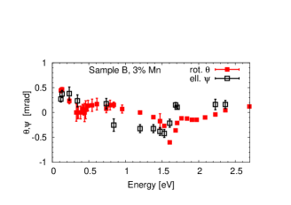
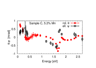
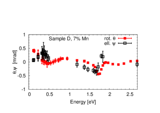
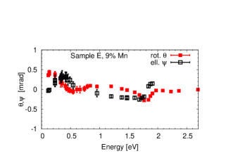
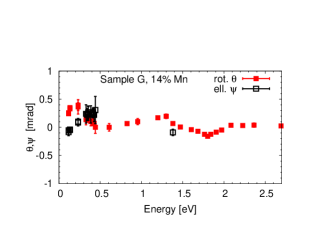
Figure 3: Measured spectral dependence of the rotation $\theta$ and ellipticity $\psi$ for the Voigt effect in reflection. Manganese doping levels indicated correspond to $x_{\mathrm{nom}}$.

IV Interpretation of the measured magneto-optical signals

To understand observed spectral features in $\theta(\omega)$ and $\psi(\omega)$ of the Voigt effect in reflection and their trends across the set of samples, a model of the electronic bands close ($\sim\hbar\omega$) to the Fermi energy $E_{f}$ is needed. Any model having ambitions to yield quantitative information on $\theta(\omega)$, $\psi(\omega)$ has to start from a description of the (Ga,Mn)As electronic structure reflecting the GaAs host bands, exchange-splitting of the bands in the ferromagnetic state of (Ga,Mn)As and the spin-orbit coupling. Without the last two components, only positions of spectral features in $\theta(\omega)$, $\psi(\omega)$ can be anticipated but not their shape and amplitude. GaAs host band structure in Fig. 1(b), calculated by standard $spds^{*}$ tight-binding modelJancu et al. (1998), suggests that the prominent peak around 1.7 eV seen in $\theta(\omega)$ of Fig. 3 corresponds to transitions between valence and conduction band. To analyze its amplitude, we have to account for the combined effect of the exchange-splitting and the spin-orbit interaction. Unlike other approaches such as the quantum defect methodBebb (1969) used in Ref. Chapler et al., 2013 to analyze absorption spectra of (Ga,Mn)As, the kinetic-exchange model of disordered carrier bandsDietl et al. (2000); Abolfath et al. (2001) which we briefly describe below, naturally includes these two components. Apart from successfully explaining the spectral trends in absorptionJungwirth et al. (2007) and of the Kerr effect in the visible range,Jungwirth et al. (2010) this model therefore allows to calculate $\theta(\omega)$, $\psi(\omega)$ of the Voigt effect in reflection which is microscopically more constrained than the absorption or the visible range Kerr effect. We show below that results of this model are in semi-quantitative agreement with the measured data as in the previously explored infrared Kerr effectAcbas et al. (2009) which also depends sensitively on the spin-orbit coupled exchange-split nature of the valence band.

The path to theoretically evaluated $\theta(\omega)$, $\psi(\omega)$ involves three steps, the first of which is to obtain the band structure $E_{\vec{k},a}$. Two of the aforementioned band structure description components are included in $\hat{H}_{KL}$ (host band structure and spin-orbit interaction), the last component (ferromagnetic exchange-splitting) enters the total Hamiltonian through kinetic-exchange parametrized by $J_{pd}$ ($J_{sd}$) couplings between the dominantly $p$-like valence band ($s$-like conduction band) and Mn $d$-levels:

$$\hat{H}=\hat{H}_{KL}+\frac{J_{pd}}{\mu_{B}}\vec{M}\cdot\hat{s}_{h}+\frac{J_{sd}}{\mu_{B}}\vec{M}\cdot\hat{s}_{e}+\hat{V}_{xc}.$$ (1)

Here, $\hat{s}_{e/h}$ is the electron/hole spin operator, $\mu_{B}$ the Bohr magneton and $\hat{V}_{xc}$ the correction due to many-body effects which is important in heavily-doped semiconductors as discussed below Eq. (7). The choice of bands included in the Kohn-Luttinger Hamiltonian $\hat{H}_{KL}$ is dictated by the energy range ($\hbar\omega$ up to 2.7 eV) in our experiments and $E_{f}$ of at most few 100 meV from the valence band top. As seen in Fig. 1b, only conduction band, heavy holes (HH), light holes (LH) and split-off band can be involved in optical excitations from occupied to unoccupied states making up the total number of eight bands in $\hat{H}_{KL}$. Parameters entering this $8\times 8$ matrix are given in Appendix C. The magnetization $\vec{M}$ that determines the ferromagnetic splitting in Eq. (1) includes only the Mn magnetic moments, hence the contribution of carrier spins must be subtracted from the saturation magnetization. We use procedure described in Appendix C below Eq. (19).

Second step is to calculate the conductivity tensor components. We take $\vec{M}\parallel\hat{x}$ and since $\sigma_{yz}$ has a negligiblenot (c) effect on $\theta$, we only need to determine $\sigma_{xx}(\omega)$ and $\sigma_{zz}(\omega)$ which we henceforth denote by $\sigma_{\parallel}$ and $\sigma_{\perp}$. They comprise of intra- and inter-band contributions,

$$\sigma_{\parallel/\perp}(\omega)=\sigma_{\parallel/\perp}^{\mathrm{intra}}+\sigma_{\parallel/\perp}^{\mathrm{inter}}.$$ (2)

where the former is simply taken as the Drude ac conductivity and the latter is calculated from the Kubo linear-response formula whose input are the energies $E_{\vec{k},a}$ and eigen-spinors $|n,\vec{k}\rangle$ obtained by numerical diagonalization of the $8\times 8$ Hamiltonian (1). Formulae for both $\sigma^{\mathrm{intra}}$ and $\sigma^{\mathrm{inter}}$ are given in the Appendix C. Complex effective permittivity $\varepsilon_{\mathrm{eff}}$ then follows from Maxwell’s equations as discussed in Appendix A. In textbooks, its two constituent terms

$$\varepsilon_{\mathrm{eff}}\equiv\varepsilon_{0}\left(\varepsilon_{b}+\frac{i\sigma}{\omega\varepsilon_{0}}\right).$$ (3)

are usually ascribed to bound and free charges. This distinction is certainly not a sharp one in the ac regime and more so at optical frequencies. The ambiguity is naturally resolved by accounting for all inter-band transitions between the eight selected bands in $\sigma$ while all other processes, at lower as well as at larger energies $\hbar\omega$, are included in the background $\varepsilon_{b}$. We include the intra-band transitions into $\sigma$ and adjust the value of $\varepsilon_{b}$ so that for intrinsic GaAs ($p=0$), $\varepsilon_{\mathrm{eff}}$ calculated using Eq. (3) recovers the experimental ac permittivity at optical frequenciesLautenschlager et al. (1987) and it approaches $\varepsilon_{\infty}=10.9$ in the $\omega\to 0$ limit. Experimentally,Johnson et al. (1969) the permittivity of intrinsic GaAs approaches this value above the optical phonon resonance ($\hbar\omega\approx 30\ \mathrm{meV}$) which is well below the lowest energies studied in our experiments.

Calculation of the rotation and ellipticity angles is the last step. Using the effective permittivity $\varepsilon_{\mathrm{eff}}^{\parallel}$ ($\varepsilon_{\mathrm{eff}}^{\perp}$) obtained from $\sigma_{\parallel}$ ($\sigma_{\perp}$), we calculate the refractive indices $n_{\parallel}$ and $n_{\perp}$ as the square root of the permittivity (see also Appendix D). When multi-reflection effects on the sample-substrate interface are neglected, we use Fresnel’s formula

$$r(n)=\frac{1-n}{1+n}$$ (4)

to get reflection coefficients $r(n_{\parallel})$ and $r(n_{\perp})$ and then calculate an auxiliary (complex-valued) quantity

$$\chi=\frac{r(n_{\parallel})-r(n_{\perp})}{r(n_{\parallel})+r(n_{\perp})}.$$ (5)

The rotation and ellipticity angles for the Voigt effect in reflection are

$$\theta=\frac{1}{2}\mbox{atan }\left(\frac{2\mbox{Re }\chi}{1-|\chi|^{2}}\right)\qquad\psi=\frac{1}{2}\mbox{asin }\left(\frac{2\mbox{Im }\chi}{1+|\chi|^{2}}\right).$$ (6)

The relationship between conductivities and actual experimentally measured angles $\theta$, $\psi$ is thus markedly non-linear, yet as a rough guide, the Voigt effect in reflection can be related to $\sigma_{\parallel}-\sigma_{\perp}$ as explained in the simplified situation pertaining to Eq. (15) in Appendix A and an example of $\sigma_{\parallel}-\sigma_{\perp}$ is shown in Fig. 11. For most of our calculations, we take the multi-reflections into account and use Eq. (33) instead of Eq. (4). Discussion of their importance is given in Appendix D.

To address experimental findings in Fig. 3, we calculate $\theta(\omega)$ of Eq. (6) in the range $\hbar\omega=0.1$ to $3.3$ eV. Such optical transition energies somewhat exceed the range of applicability of our band structure model in Eq. (1); eight band $k\cdot p$ model does not describe the conduction band bending between $\Gamma$ and $L$ points that can be seen in Fig. 1(b). Transitions between valence and conduction band in the $L$-point that will contribute to $\sigma(\omega)$ at latest around $\hbar\omega=3$ eV are absent in our model calculations. However, strong experimental magneto-optical signals in Fig. 3 all appear below $\hbar\omega=2$ eV and $L$-point transitions should be unimportant for such energies (see again Fig. 1b). In the calculations we consider an extended range of $\hbar\omega$ up to $3.3\ \mathrm{eV}$ to show features which, as we explain below, would be shifted in realistic materials with strong disorder to lower energies. The two basic sample parameters that enter our model are the carrier (hole) density $p$ and the effective doping $x$, see Eq. (19), that determine primarily the Fermi level $E_{f}$ and ferromagnetic splittings in Eq. (1), respectively. Given the span of $p$ and $x$ in Tab. 1, we first show in Fig. 4 calculated $\theta(\omega)$ for fixed $x=5\%$ and varying $p$ (panel a) and fixed $p=0.8\ \mathrm{nm^{-3}}$ and varying $x$ (panel b). The order of magnitude of $\theta(\omega)$ and its structure agrees with experimental data in Fig. 3. We discuss and compare the individual spectral features in more detail below and for convenience, we label three of them by Greek letters $\alpha$, $\beta$ and $\gamma$ as shown in Fig. 4a. We begin our discussion by identifying the optical transitions which are responsible for the individual spectral features. Before that, we just briefly remark that $\theta(\omega)$ comprises both MLB and MLD contributions as we demonstrate in a simple example below Eq. (32) in Appendix D.

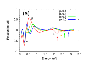
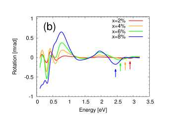
Figure 4: Calculated spectral dependence of the rotation angle $\theta$ with $\hat{V}_{xc}=0$ for a series of systems with (a) $x=5\%$ and varying $p$ (in$\ \mathrm{nm^{-3}}$) and (b) varying $x$ and constant $p=0.8\ \mathrm{nm^{-3}}$. Spectral features discussed in text are labelled by Greek letters, arrows indicate the position of peak $\alpha$.

The conductivity that enters the rotation via reflection coefficients in Eq. (5) can be decomposed into contributions of individual bands. The relationship between $\theta$ and tensor components of $\sigma$ is non-linear, yet it turns out that the individual summands in $\sigma(\omega)$, see Eq. (22), give rise to well-defined structures in $\theta(\omega)$. The bottom panel in Fig. 5 demonstrates that peak $\alpha$ arises because of optical transitions from the LH and HH bands (H) to the conduction bands (C), peak $\beta$ is mostly due to transitions between the split-off bands (S) and H while the intra-H transitions underlie peak $\gamma$. The intra-band contribution to $\sigma$ has, according to the top panel of Fig. 5, almost no perceptible influence on the resulting $\theta(\omega)$, except for the lowest energies ($\hbar\omega\approx 100$ meV). Sources of the weak anisotropy of $\sigma^{\mathrm{intra}}$ are discussed in Appendix C below Eq. (21).

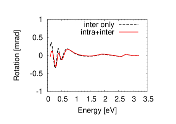
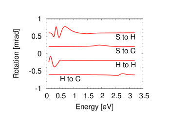
Figure 5: Decomposition of $\theta(\omega)$ into individual terms appearing in the ac conductivity for $x=3\%,p=0.6\ \mathrm{nm^{-3}}$. Top: $\theta(\omega)$ with and without intraband terms in Eq. (2). Bottom: $\theta(\omega)$ calculated only using selected interband transitions in Eq. (22) (H=hole bands, C=conduction bands, S=split-off bands). Calculated data in the bottom panel are vertically offset.

The feature $\alpha$ seen consistently both in the model calculations (Fig. 4) and experimental data (Fig. 3) is thus largely due to optical transitions across the gap. Although our model underestimates the effect of disorder in (Ga,Mn)As, this conclusion is independent of the strength of disorder. Let us take amorphous GaAs as an extreme example of a disordered system. Despite the completely destroyed translational symmetry, optical properties such as photoemission spectra remain largely the same as for perfect crystals. Important property of the amorphous material underlying this similarity is the chemical bonding which is not very different from the perfect crystal. Amorphous GaAs retains the so called Tauc optical gapda Silva et al. (2004); Tauc et al. (1966) of the order of $E_{g}$. The orbital character of states below the gap remains similar to the perfect crystal and the main changenot (d) between the perfect crystal and amorphous material, using the language of the former material, will be the presence of non-direct, $\vec{k}$ non-conserving, transitions in the amorphous material. We prefer the term ”non-direct” to ”indirect” to avoid confusion with phonon-mediated transitions. Since disorder generally tends to reduce the gapda Silva et al. (2004) and positions of peak $\alpha$ in our experiments are consistently above the band-gap in the perfect GaAs crystal ($E_{g}$), it implies that Fermi level in our samples lies in the valence band as it is commonly assumed.Jungwirth et al. (2007) This conclusion is also supported by a blue shift of peak $\alpha$ with increasing $x$, suggestive of the Moss-Burstein shift.Moss (1954) From the point of view of our model and with the help of the bottom panel of Fig. 5, peak $\alpha$ in $\theta(\omega)$ arises from the direct transitions from states at Fermi wavevector in H to states at the same wavevector in C. Such transitions are shown by the vertical arrow labelled A in Fig. 1b. Technically, the apparent conservation of wavevector in a disordered system is a consequence of averaging over impurity configurations (velocity operator matrix elements in Eq. (22) are diagonal in $k$). To some extent, the non-conservation of the wavevector is captured by the imaginary part of the self-energy $\Gamma$ (see Appendix C) but this is, strictly speaking, only a correction justified in the weak-disorder regime. Given the relatively low sheet conductivities of our samples,Jungwirth et al. (2010) disorder corrections to Eqs. (22,31) may be sizable and the effect of non-direct transitions on $\sigma^{\mathrm{inter}}$ larger than what is implied by Eq. (22).

The direct transitions H$\to$C from the Fermi surface appear around $\hbar\omega\approx E_{g}+|E_{f}|(1+m_{H}/m_{C})$ where, for the sake of illustration, we describe valence (conduction) bands by a single effective mass $m_{H}$ ($m_{C}$). This energy rapidly increases with increasing $E_{f}$, i.e., with increasing hole density which in the studied optimized (Ga,Mn)As samples is a monotonic increasing function of $x_{\mathrm{nom}}$. This blue shift is so rapid for HHs ($m_{H}/m_{C}\sim 10$) that the corresponding spectral feature is even out-of-range in Fig. 4. The actual transitions responsible for peak $\alpha$ are those from the LHs to C ($m_{H}/m_{C}\sim 1$ by the order of magnitude) and even so, the blue shift of the peak turns out to be much faster than what is observed experimentally as we explain below (see also Fig. 8). We return to the non-direct transitions later and now discuss another possible reason for the too high energies of the $\alpha$ peak in Fig. 4 as compared to the corresponding spectral feature in the experimental Fig. 3.

Our (Ga,Mn)As samples are very heavily doped from the perspective of traditional semiconductors, electron-electron interactions can therefore appreciably contribute to the total energy.not (e) Indeed, the exchange energy per particle of free spin-polarized electrons,

$$E_{x}/N=-\frac{e^{2}}{4\pi\epsilon}\frac{3k_{F}}{4\pi}$$ (7)

is of the order of 100 meV at carrier densities of the order of $10^{21}\ \mathrm{cm^{-3}}$. The difficulty in evaluating the exchange-correlation effects for the holes is in the presence of a strong spin-orbit coupling. One possible approximative scheme is discussed in Ref. Sipahi et al., 1996. To assess the qualitative effect of exchange energy on trends in the rotation spectra of the Voigt effect in reflection, we use the following scheme. We first disregard the correlation effects which are small compared to exchange in Eq. (7). For given $x$ and $p$, we first determine the band occupations by holes $p_{i}$ ($\Sigma_{i}p_{i}=p$, $i=1,\ldots,6$) as given by Eq. (1) with $V_{xc}=0$. For most of the considered dopings, only the LH ($i=3,4$) and HH bands ($i=5,6$) are occupied by holes. We next recalculate the corresponding densities $p_{i}$ into Fermi wavevectors assuming isotropic dispersion and shift the bands by $-E_{x}/N$ as given by Eq. (7). Since $-E_{x}/N$ is different for different bands, this procedure not only renormalizes the Fermi level but also slightly changes $p_{i}$ and therefore we iterate the procedure until we converge to a consistent set of $p_{i}$ and exchange shifts. Note that we neglected in this procedure the exchange between bands $i\not=j$. To justify this approximation, at least in part, we checked the spin-polarizations of individual bands. For example, $x=3\%$, $p=0.6\ \mathrm{nm^{-3}}$ leads to $p_{3,4,5,6}/p=0.02,0.04,0.33,0.61$ and integral spin polarizations $2\langle s\rangle_{3,4,5,6}=0.58,-0.14,0.57,-0.91$. The majority HHs are thus prevalent and nearly completely polarized, hence their exchange interaction with holes in other bands will be small and our estimate using Eq. (7) with $k_{F}^{3}=6\pi^{2}p_{6}$ should be a good approximation. On the other hand, the exchange shifts for LH bands may contain sizable corrections due to the neglected inter-band exchange and the values 52, 62, 126 and 154 meV thus serve only as a rough guide to assess many-body effects on the magneto-optical spectra. These values are similar to the band gap renormalizationZhang and Das Sarma (2005) used previously.Acbas et al. (2009) A commonly considered correction to Eq. (7) capturing part of the correlation effects is logarithmic and weakly dependent on $p$ in our range of parameters. Appealing to the second term in Eq. (36) of Ref. Sipahi et al., 1996 and the procedure described therein, we include it into our model through a small constant shift of 6.5 meV (1.5 meV) for HH (LH) bands towards the conduction bands. To summarize many-body corrections included in Eq. (1), $\hat{V}_{xc}$ can be understood as a single-particle operator that commutes with $\hat{H}$ and shifts the selected bands as just described to account for exchange and partly also correlations. This approximative treatment enhances the ferromagnetic splitting between minority and majority hole bands and also adds an additional offset between the HH and LH bands.

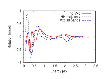
Figure 6: Rotation $\theta(\omega)$ under various approximations to $\hat{V}_{xc}$ for $x=5\%$, $p=0.8\ \mathrm{nm^{-3}}$. Note the position of the $\alpha$-peak: it appears at a relatively large energy for $\hat{V}_{xc}=0$ (”no Vxc”, corresponds to Fig. 4) and shifts to lower energies when electron-electron exchange energy is taken into account. Adopting the approach of Ref. Acbas et al., 2009 (”HH maj. only”), we find the peak $\alpha$ around $2.3\ \mathrm{eV}$ and when applying the exchange shift to all bands (corresponds to Fig. 7), it shifts down to $2.1\ \mathrm{eV}$.

Although the spectra with and without exchange-correction effects are qualitatively similar, there are some notable differences. We observe a significant amplification and red shift of the peak $\alpha$ by hundreds of meV, depending on the approximation as shown in Fig. 6, and the double maximum structure around and above $\hbar\omega=0.5\ \mathrm{eV}$ tends to merge into a single $\beta$-peak structure. Absence of the double maximum in the range 0.5–1.2 eV in experimental data of Fig. 3 suggests that $\hat{V}_{xc}$ may be an important ingredient in the model. The peak $\alpha$ — now at smaller energies — follows the same trends as with $\hat{V}_{xc}=0$: it blue shifts with increasing $p$ and red shifts with increasing $x$ as shown in Fig. 7. We checked these trends with the model of $\hat{V}_{xc}$ used previously by some of us for calculating magneto-optical effects odd in magnetizationAcbas et al. (2009) where only majority HH band is exchange-shifted. To give an impression, we display the corresponding spectrum as the dotted line in Fig. 6. Finding the trends independent of the approximation used for $\hat{V}_{xc}$, we proceed to use from now on the exchange shifts as described below Eq. (7) which lead to $\theta(\omega)$ shown by dashed line in Fig. 6.

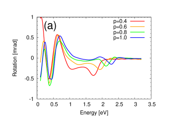
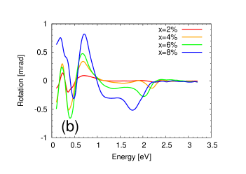
Figure 7: Calculated spectral dependence of the rotation angle $\theta$, the same as Fig. 4 but with $\hat{V}_{xc}$ taken into account as it is described below Eq. (7).

Even with the many-body band renormalization effects included, the peak $\alpha$ still lies at considerably higher energy (above $2\ \mathrm{eV}$) than what is observed experimentally (around $1.7\ \mathrm{eV}$ in Fig. 3). We summarize its position in Fig. 8. Experimental data from Fig. 3 (crosses in Fig. 8) and independent measurements described in Appendix B (empty boxes in Fig. 8) consistently show a slow blue shift with increased nominal doping but the rate of this shift with $x_{\mathrm{nom}}$ is much slower than what the mean-field kinetic-exchange model predicts. This is pointing to a shortcoming of our electronic-structure model represented by Eq. (1) where the presence of Mn is effectively treated in a mean-field virtual-crystal approximation. At the level of the Kubo formula in Eq. (22), our model only allows for direct transitions and below we continue the discussion about how the experimental values of the peak $\alpha$ positions could possibly be explained by considering non-direct transitions and electrostatic interaction between holes and ionized acceptors.

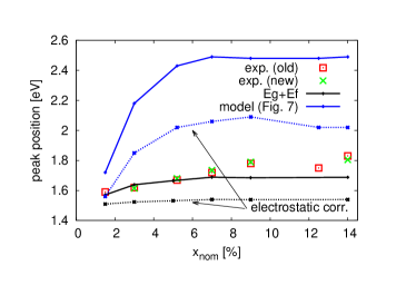
Figure 8: Positions of the $\alpha$-peak for the series of samples described by Tab. 1. Old and new experimental data correspond to results obtained by different techniques, peak positions were extracted from $\theta(\omega)$ data in Fig. 3 (new) and from measurements below and above $T_{c}$ described in Appendix B (old). Model data (solid blue line) take into account direct transitions only, the extreme limit of non-direct transitions (solid black) corresponds to $E_{g}+E_{f}$ where $V_{xc}$ is also included. Dotted lines show these two limiting cases when electrostatic interaction with ionized acceptors is considered.

Treating a realistic band-structure and disorder on equal footing is a complicated task and we therefore discuss the effect of the latter only qualitatively. It is important to keep in mind that the disorder broadening $\Gamma$ which appears in the Kubo formula (22) is only a poor approximation to the non-conservation of wavevector $\vec{k}$ in the strong-disorder case. Due to disorder in the crystal caused primarily by random positions of Mn atoms substituting for the cations of the host lattice, the Bloch theorem does not apply and $\vec{k}$ is not a good quantum number. However, even in the extreme case of an amorphous continuous covalent network discussed above, the valence and conduction bands are largely preserved although the gap between them may be smallerda Silva et al. (2004) than the perfect-crystal value $E_{g}$. The lowest-energy optical transition would then appear close to energy $E_{f}+E_{g}$ corresponding to the arrow labelled B in Fig. 1b if we use the language of non-direct transitions for the perfect-crystal band structure. In some sense, this could be understood as calculating the band structure from Eq. (1) and then replacing the matrix elements in Kubo formula (22) by an expression that completely ignores $\vec{k}$ as opposed to matrix elements diagonal in $\vec{k}$. Such estimate of the position of peak $\alpha$ is its lower bound provided that we use the proper value of $E_{g}$ reduced by the disorder.da Silva et al. (2004) This lower-bound property turns out to apply to our experimental data even if we use the perfect-crystal value of $E_{g}$ reduced by $V_{xc}$ for majority HH as it is shown in Fig. 8 by the solid black curve. Admittedly, the experimental data are very close to this lower bound.

An effect that we have ignored in our discussion so far is the electrostatic interaction between delocalized holes and ionized Mn acceptors. The charge density of the latter is not constant as in the jellium model and this causes an additional band-gap renormalization that can be described by the real part of self-energy due to hole-acceptor scattering.Zhang and Das Sarma (2005) We estimate it by Eq. (5) of this reference with $g=1$ (full spin-polarization of the holes) and HH effective mass of half the free electron mass as an additional shift of the valence bands towards the conduction bands added to $\hat{V}_{xc}$. Positions of the peak $\alpha$ red shift by additionalJungwirth et al. (2010) $\sim 300\ \mathrm{meV}$ as shown in Fig. 8 by the dotted blue line. For completeness, we also show by dotted black line $E_{g}+E_{f}$ with $\hat{V}_{xc}$ included as well as the effect of band-gap renormalization due to the ionized Mn acceptors described by Eq. (5) in Ref. Zhang and Das Sarma, 2005. At this level, we can conclude that since the experimental data lie approximately half-way between the lower and upper bounds delimited by the dotted lines in Fig. 8, the non-direct transitions might play a significant role in optical transitions but band renormalizations due to exchange-correlation and hole-acceptor electrostatic interaction effects are also sizable. Quantitative modelling of experimental magneto-optical data would require rigorous quantitative description of all these effects.

Returning to our model of direct transitions only, the experimental feature where it performs relatively poorly are the peak amplitudes. Although the predicted order of magnitude is correct (0.1 mrad for all peaks $\alpha,\beta,\gamma$ in Figs. 4,7), it is notable that $\alpha$ is smaller than both $\beta$ and $\gamma$ while the same peak $\alpha$ is by far the largest in experiments summarized in Fig. 3. Smaller amplitude of peaks $\beta,\gamma$ together with possibly larger linewidth in experiment may be a consequence of disorder-induced non-direct transitions which are not included in our model. Beyond the very crude treatment of the chemical aspect of disorder in our model,not (d) we speculate that translational symmetry breaking underlies the differences between the model and experiment also in the case of peak $\alpha$. Our model shows that the amplitude monotonically grows with $x$ across our set of samples. This is understandable since all magneto-optical effects must vanish in the limit $x\to 0$ and actually, this decay is seen in experimental data for samples C,B,A in Fig. 10b. (We disregard the small magneto-optical effects in non-magnetic GaAs which are present at finite magnetic fields.Ando et al. (1998)) On the other hand, disorder might play larger role at higher doping concentrations in metallic samples sufficiently far from the metal-insulator transition hence the decrease of peak $\alpha$ heights for samples C,D,E. We note that the experimentally determined extraordinarily largeBuchmeier et al. (2009) height of peak $\alpha$ ($-0.86$ mrad) is about three times larger than the result of the model based on Eq. (1) (see Fig. 9a). It is possible that a more refined choice of the scattering rates, instead of a single parameter $\Gamma$ (see Appendix C), could reduce this difference but such analysis is beyond scope of this article.

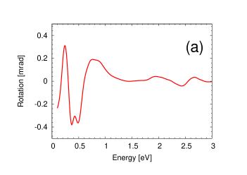
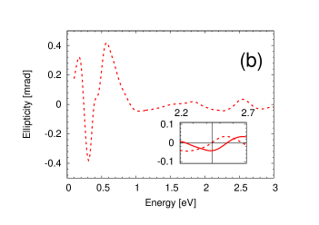
Figure 9: Spectral dependence of (a) rotation and (b) ellipticity for $x=3.6\%$, $p=1.08$, with $\hat{V}_{xc}$ included. These parameters correspond to sample C ($x_{\mathrm{nom}}=5.2\%$). The inset shows detail of rotation (solid) and ellipticity (dotted) around peak $\alpha$.

We finally comment on the spectral dependence of ellipticity $\psi(\omega)$ which can also be readily calculated using Eq. (6). Since the ellipticity is experimentally somewhat more difficult to access,Tesařová et al. (2012) less data than for $\theta(\omega)$ is available and we keep the following discussion short. Let us compare Fig. 9 to sample C in Fig. 3. Our model gives the correct order of magnitude and functional shape of ellipticity related to the peak $\alpha$ in rotation. The inset of Fig. 9b clearly shows that Lorentzian peak $\alpha$ in rotation corresponds to an anti-Lorentzian one in ellipticity which is found again in experimental data. Regarding other spectral features in ellipticity, we find a minimum close to $\hbar\omega=300\ \mathrm{meV}$ in Fig. 9b while no such feature is observed experimentally. Given the complicated structure of the valence bands and large shifts of the $\alpha$-peak ascribed to disorder as discussed above, we will not attempt to speculate on how this feature could be suppressed and only note that the experimental magnitude of $\psi\approx 0.4\ \mathrm{mrad}$ is similar to calculations in Fig. 9b. Our model can therefore capture only semi-quantitatively the major trends seen in the experimental magneto-optical data.

V Conclusions

Rotation $\theta(\omega)$ and ellipticity $\psi(\omega)$ measured for the Voigt effect in reflection, a direct consequence of the magnetic linear dichroism and birefringence, represent a much more sensitive spectroscopic probe into the electronic structure of (Ga,Mn)As than, for instance, unpolarized optical absorption experiments. Our measured data are compatible with the previously published $\theta(\omega)$ on selected samples and limited spectral range and we investigate variations of the spectra with manganese doping which influences both the exchange-splitting and Fermi level. We confirm that $\theta$ at energies exceeding the gap of the GaAs host can reach values larger than so far reported in other ferromagnetic materials. The corresponding peak is found to blue shift with increasing manganese doping and we analyse this trend using the $k\cdot p$ mean-field kinetic-exchange model. We find that even with exchange-correlation band renormalization effects taken into account, this model yields appreciably larger energies at which this feature is seen, compared to experiment, and we attribute this fact to the neglected of non-direct transitions caused by the disorder. Apart from this deficiency, the model correctly reproduces the structure of experimental $\theta(\omega)$ and $\psi(\omega)$ ranging from $112$ meV to $2.7$ eV, captures the sign of the peaks and, semi-quantitatively, also their amplitude. A more quantitative description of the measured magneto-optical spectra would require to combine the modeling of the complex, spin-orbit coupled band structure with a more detailed treatment of the strong disorder effects in (Ga,Mn)As, as previously done, e.g., in the studies of unpolarized absorption spectra.Yang et al. (2003)

Appendix A Classical theory of magneto-optical effects

Maxwell’s equations allow to show how the magneto-optical effects described in Sec. II follow from properties of the bulk magnetic material. Inspired by the argumentation of Ref. Osgood III et al., 1998, we review in this Appendix how MLD/MLB (or their circular counterparts), i.e. difference in imaginary/real parts of the refractive indices for two linearly (circularly) polarized modes, is calculated from bulk ac conductivity tensor of the material. Relation between these refractive indices and the particular magneto-optical effects is also explained here using simple examples and we refer the reader to Appendix D for a discussion of the more realistic relationship pertaining to our measurements.

Consider an electromagnetic wave $\vec{E}(\vec{r},t)=\vec{E}_{0}e^{i(kz-\omega t)}$ propagating along $\vec{k}\parallel\hat{z}$. The non-zero ac conductivity $\sigma(\omega)$ and Maxwell equations imply that

$$\nabla(\nabla\cdot\vec{E})-\nabla^{2}\vec{E}=-\mu\sigma\dot{\vec{E}}-\mu\varepsilon\ddot{\vec{E}}$$ (8)

which yields an equation for $\vec{E}_{0}$ whose solutions correspond to propagating modes when $n^{2}\equiv(ck/\omega)^{2}>0$ where $c$ is the light velocity. Character of these modes depends on the form of the permeability $\mu$, permittivity $\varepsilon$ and conductivity $\sigma$ tensors. The right-hand-side of Eq. (8) takes on the form $\omega^{2}\mu\varepsilon_{\mathrm{eff}}\vec{E}(\vec{r},t)$ where $\varepsilon_{\mathrm{eff}}$ can be written as $\varepsilon_{0}+i\sigma/\omega$ if we replace $\varepsilon$ by vacuum permittivity $\varepsilon_{0}$ or as in Eq. (3), depending on how the ambiguity discussed below Eq. (3) is resolved. We obtain the modes by solving Eq. (8) and their $\vec{E}_{0}$ and refractive indices $n$ depend on the form of the effective permittivity tensor $\varepsilon_{\mathrm{eff}}$. We now consider two examples related to the magnetization-in-plane and out-of-plane magneto-optical experiments discussed in Sec. II. The permeability $\mu$ will from now on be considered a scalar equal to the vacuum permeability and a material of cubic symmetry will be assumed whose index of refraction in the absence of magnetization equals $n_{0}=\sqrt{\varepsilon_{\mathrm{eff}}/\varepsilon_{0}}$.

In the first example, $\vec{M}\parallel\hat{z}$ which impliesnot (f) an effective permittivity tensor of the form

$$\varepsilon_{\mathrm{eff}}=\varepsilon_{0}\left(\begin{array}[]{ccc}\varepsilon_{xx}&\varepsilon_{xy}&0\\ -\varepsilon_{xy}&\varepsilon_{xx}&0\\ 0&0&\varepsilon_{zz}\end{array}\right)$$ (9)

with dimensionless components $\varepsilon_{ij}$. The eigenmodes obtained by solving Eq. (8) are two circularly polarized waves with

$$\left(\begin{array}[]{c}E_{x}^{0}\\ E_{y}^{0}\\ E_{z}^{0}\end{array}\right)\propto\left(\begin{array}[]{c}1\\ i\\ 0\end{array}\right)\mbox{ and }\left(\begin{array}[]{c}1\\ -i\\ 0\end{array}\right)$$ (10)

for $n^{2}_{+}=\varepsilon_{xx}+i\varepsilon_{xy}$ and $n^{2}_{-}=\varepsilon_{xx}-i\varepsilon_{xy}$. Let us now explain how the Faraday effect arises in such a situation, sketched in Fig. 2a. Consider a slab of a magnetic material of thickness $d$ described by $\varepsilon_{\mathrm{eff}}$ in Eq. (9) placed in vacuum, assume normal incidence and, for simplicity, the absence of reflections on the vacuum-sample surface. An incoming linearly polarized wave with $\vec{E}_{0}=(E_{x}^{0},0,0)$ will propagate through the sample in two circularly polarized modes at different group velocities. Under the additional (typically satisfied) assumption $|n_{\pm}-n_{0}|\ll n_{0}$, we can conclude using

$$n_{+}-n_{-}\approx\frac{n_{+}^{2}-n_{-}^{2}}{2n_{0}}=\frac{i\varepsilon_{xy}}{n_{0}}$$ (11)

that the polarization plane of the outgoing wave will be rotated by $\theta\approx-(d\omega/c)\mbox{Im }\varepsilon_{xy}/n_{0}$. In this transmission geometry (and under the simplifying assumption on surface reflections), the Faraday rotation is directly related to magnetic circular birefringence (MCB) while magnetic circular dichroism (MCD) will make the outgoing wave elliptically polarized ($\psi\not=0$).

The (polar) Kerr effect is obtained by considering reflection off an interface between a semi-infinite magnetic material and vacuum. The Fresnel formula (4) for the reflection coefficient $r$ at normal incidence (ratio of outgoing to incident beam’s $E_{x}^{0}$) reads $r=(1-n)/(1+n)$ and applying it to $n_{\pm}$ defined below Eq. (10), we obtain $r_{\pm}$ for the two circularly polarized modes. For $r_{+}/r_{-}=ae^{i\xi}$ (with $a,\xi$ real), the originally linearly polarized wave will be reflected as elliptically polarized (unless $a=1$) with the major axis rotated by $\theta=\xi$ (see Fig. 1). In a general case, it is not possible to link MCB alone directly to the rotation and unlike with the Faraday effect, both MCB and MCD will influence $\theta$ because the relation between $r$ and $n$ is non-linear. An illustrative example of this is given in Appendix D.

In the second example $\vec{M}\parallel\hat{x}$, which implies the same form of $\varepsilon_{\mathrm{eff}}$ as in Eq. (9) up to a permutation of indices:

$$\varepsilon_{0}\left(\begin{array}[]{ccc}\varepsilon_{xx}&0&0\\ 0&\varepsilon_{zz}&\varepsilon_{yz}\\ 0&-\varepsilon_{yz}&\varepsilon_{zz}\end{array}\right).$$ (12)

Solving Eq. (8) for $\vec{E}_{0}$ gives

$$\left(\begin{array}[]{c}E_{x}^{0}\\ E_{y}^{0}\\ E_{z}^{0}\end{array}\right)\propto\left(\begin{array}[]{c}1\\ 0\\ 0\end{array}\right)\mbox{ and }\left(\begin{array}[]{c}0\\ 1\\ \varepsilon_{yz}/\varepsilon_{zz}\end{array}\right)$$ (13)

with refractive indices $n_{\parallel}^{2}=\varepsilon_{xx}$ and $n_{\perp}^{2}=\varepsilon_{zz}[1+(\varepsilon_{yz}/\varepsilon_{zz})^{2}]$. Voigt rotation (after transmission through a slab of the magnetic material as sketched in Fig. 2b) is related to

$$n_{\parallel}-n_{\perp}\approx\frac{1}{2}n_{0}(\varepsilon_{xx}-\varepsilon_{zz}-\frac{\varepsilon_{yz}^{2}}{\varepsilon_{zz}})$$ (14)

in analogy to Eq. (11) and polarization plane rotation in the Voigt effect in reflection (assuming $\beta=\pi/4$ and $b=r_{\parallel}/r_{\perp}$ real for simplicity) follows from

$$\tan\theta=\frac{1-b}{1+b}\approx\frac{n_{0}}{2(n_{0}^{2}-1)}(\varepsilon_{xx}-\varepsilon_{zz}-\frac{\varepsilon_{yz}^{2}}{\varepsilon_{zz}}).$$ (15)

For other mutual positions of $\vec{M}$ and polarization plane, $\theta$ will follow the $\sin 2\beta$ dependence as mentioned in Sec. II. In particular, when incident beam polarization is parallel or perpendicular to $\vec{M}$, light in the magnetic material travels simply as the first or second mode in (13) and the polarization remains unchanged.

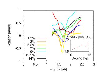
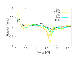
(a)	(b)

Figure 10: Overview of the measured rotation angle $\theta$ for samples A–G using (a) the subtraction of data above $T_{c}$ and (b) the in situ rotation of $\vec{M}$. Inset in panel (a) shows the position in eV of the peak $\alpha$ as a function of Mn doping. All Mn concentrations indicated are $x_{\mathrm{nom}}$ (see Tab. 1).

With these two examples at hand, we can make several observations. Recall that we have always considered the normal incidence here. The in-plane magnetization leads to magneto-optical effects even in magnetization, $\theta(\vec{M})=\theta(-\vec{M})$, as stated in Sec. II. In Eq. (14), $\varepsilon_{xx}-\varepsilon_{zz}$ is even in $\vec{M}$ owing to the Onsager relations, and $\varepsilon_{yz}^{2}$ is even because $\varepsilon_{yz}(\vec{M})$ is odd.not (g) Next, we can see that a non-zero difference between $n_{\parallel}$ and $n_{\perp}$ in non-dissipative systems ($\mbox{Im }n_{\parallel}=\mbox{Im }n_{\perp}=0$), a circumstance that could be called ”pure MLB”, causes rotation in the Voigt effect in reflection. However, as soon as $n_{\parallel}$ and $n_{\perp}$ are complex, both MLB and MLD will influence $\theta$ because of the non-linear dependence of $r$ on $n$ in Eq. (4). We again refer to the illustrative example given in Appendix D. Similar statement holds about ellipticity of the Voigt effect in reflection. Some confusion can arise because of different terminology used in the literature: Ref. Ferre and Gehring, 1984 relates MLB to the real part of refractive indices while Ref. Kimel et al., 2005 to the real part of the reflection coefficients. We find the former terminology more appropriate because it is generic for both reflection and transmission coefficients. Independent of the terminology, it is safe to state that different complex refractive indices $n_{\parallel}$ and $n_{\perp}$ cause $\theta\not=0$, $\psi\not=0$ in both transmission and reflection experiments. Nonzero $n_{\parallel}-n_{\perp}$ arises due to difference in diagonal components of $\varepsilon_{\mathrm{eff}}$ or nonzero $\varepsilon_{yz}$, as seen in Eq. (14). Since $\varepsilon_{yz}^{2}/\varepsilon_{zz}$ is in our case negligible,not (c) one can conclude that the Voigt effect in reflection or in transmission is (via MLB and MLD) primarily driven by the difference of diagonal components of $\sigma(\omega)$ corresponding to directions parallel and perpendicular to $\vec{M}$, i.e., by the ac anisotropic magnetoresistance.

We conclude this Appendix by explaining the relationship between terminology used in this article (components of the effective permittivity tensor $\varepsilon_{\mathrm{eff}}$) and the notation of ”quadratic magneto-optic tensor components”Birss (1964); Višňovský (1986) used elsewhere.Postava et al. (2002); Bhagavantam (1966); Hamrlová et al. (2013) The basic conceptual difference between the two approaches is whether $\vec{M}$ is kept fixed and different polarizations of light are considered (the former approach) or vice versa (the latter approach). An advantage of the latter approach is its aptitude to describe the ac analogy of crystalline anisotropic magnetoresistance componentsde Ranieri et al. (2008) which we completely ignore in this article, motivated by their smallness in the dc limit.Rushforth et al. (2007) We expand the effective permittivity tensor into a Taylor series in powers of the magnetization Cartesian components $M_{k}$:

$$\varepsilon_{ij}=\varepsilon_{ij}^{(0)}+K_{ijk}M_{k}+G_{ijkl}M_{k}M_{l}+\ldots$$ (16)

where $\varepsilon_{ij}^{(0)}$ is the part independent on magnetization, $K_{ijk}$ and $G_{ijkl}$ are rank three and four tensors and the last two are sometimes also called linear and quadratic magneto-optical tensors. They represent the parts of the permittivity tensor which are linear and quadratic in magnetization, respectively.

The form of $K_{ijk}$ and $G_{ijkl}$ depends on the symmetry of the crystalVišňovský (1986) as well as on the orientation of principal crystal axis with respect to $xyz$-axis in which the permittivity tensor is expressed.Hamrlová et al. (2013) In case of cubic crystals with point symmetry (crystal classes 23=T, m3=T_h, 432=O, $\overline{4}$3m=T_d and m3m=O_h) where $\langle 100\rangle$, $\langle 010\rangle$ and $\langle 001\rangle$ are parallel with $x$, $y$ and $z$-axis, respectively, following three statements hold. Non-magnetic part of the permittivity tensor is constant, $\varepsilon_{ij}^{(0)}=\delta_{ij}\varepsilon^{(0)}$, where $\delta_{ij}$ is the Kronecker delta. The third rank tensor $K_{ijk}=\gamma_{ijk}K$ where $\gamma_{ijk}$ is Levi-Civita symbol. The rank four tensor $G_{ijkl}$ can be written in matrix form asVišňovský (1986)

$$\left(\hskip-1.42262pt\begin{array}[]{c}\varepsilon_{xx}^{(2)}\\ \varepsilon_{yy}^{(2)}\\ \varepsilon_{zz}^{(2)}\\ \varepsilon_{yz}^{(2)}\\ \varepsilon_{zx}^{(2)}\\ \varepsilon_{xy}^{(2)}\end{array}\hskip-1.42262pt\right)\hskip-2.84526pt=\hskip-2.84526pt\left(\begin{array}[]{cccccc}G_{11}&G_{12}&G_{12}&0&0&0\\ G_{12}&G_{11}&G_{12}&0&0&0\\ G_{12}&G_{12}&G_{11}&0&0&0\\ 0&0&0&2G_{44}&0&0\\ 0&0&0&0&2G_{44}&0\\ 0&0&0&0&0&2G_{44}\end{array}\right)\hskip-2.84526pt\left(\hskip-1.42262pt\begin{array}[]{c}M_{x}^{2}\\ M_{y}^{2}\\ M_{z}^{2}\\ M_{y}M_{z}\\ M_{z}M_{x}\\ M_{x}M_{y}\end{array}\hskip-1.42262pt\right)$$ (17)

where $\varepsilon_{ij}^{(2)}=G_{ijkl}M_{k}M_{l}$. In the case of an isotropic material, the number of free parameters is further reduced because $2G_{44}=G_{11}-G_{12}$.

In our analysis in Sec. IV, magnetization was always oriented along $x$-axis and combining Eq. (17) and (16), we arrive at

$$\varepsilon=\left(\begin{array}[]{ccc}\varepsilon^{(0)}+G_{11}M_{x}^{2}&0&0\\ 0&\varepsilon^{(0)}+G_{12}M_{x}^{2}&KM_{x}\\ 0&-KM_{x}&\varepsilon^{(0)}+G_{12}M_{x}^{2}\end{array}\right).$$ (18)

Repeating the analysis leading to Eq. (14), we now find $n_{\parallel}-n_{\perp}=(G_{11}-G_{12}-K^{2}/\varepsilon^{(0)})M_{x}^{2}$.

Appendix B Additional experimental data

As it is discussed in Sec. III and in Ref. Tesařová et al., 2012, a difficulty related to the measurement of magneto-optical phenomena even in $\vec{M}$ is that the actual signal cannot be separated from background simply by subtracting the results in magnetic field $B$ and $-B$. One possible approach is to subtract results at $T>T_{C}$ from those at the low temperature of interest. Phenomena related to magnetism are suppressed at $T>T_{C}$ and the remaining signal stemming from the experimental apparatus is still often large, see Fig. 3b in Ref. Tesařová et al., 2012. Our measurements using this technique are summarized in Fig. 10a (note that with this technique, we measured also samples A and F not available Fig. 3). Even between two measurements of the same sample, inferred $\theta(\omega)$ may be offset because of temperature-dependence in optical properties of measurement setup elements. On the other hand, the techniqueTesařová et al. (2012) of in situ rotating $\vec{M}$ is free of these artefacts as it is apparent from the $\theta(\omega)$ data of Fig. 3 summarized in Fig. 10b. The peak positions (given in the inset of the panel a) agree well between the two methods — compare the two sets of experimental data in Fig. 8.

Appendix C Microscopic model

This appendix contains detailed information about the model of (Ga,Mn)As electronic structure embodied in Eq. (1), its parameters and the Kubo formula used to calculate conductivity tensor components entering Eq. (2).

Individual samples are primarily characterized by the Mn doping $x$ (fraction of Ga atoms substituted by Mn) and total hole density $p$. The former is taken as $x=N_{\mathrm{Mn}}a_{l}^{3}/4$ where $a_{l}=0.565325\ \mathrm{nm}$ is the GaAs lattice constant and $N_{\mathrm{Mn}}$ is the density of Mn atoms. Since Mn substituting for a Ga atom is a single acceptor, it follows $p=N_{\mathrm{Mn}}$ and $|\vec{M}|=5\mu_{B}N_{\mathrm{Mn}}$ in the ideal case (for the moment, we neglect magnetic moment of the holes, included in Eq. (19) below). However, compensating impurities (e.g. As antisites or Mn atoms in interstitial position) will reduce both $p$ and magnetization $|\vec{M}|$. These two quantities therefore have to be determined independently by measurement as it is done in Fig. 10 and Tab. I of the Supplemental Information in Ref. Jungwirth et al., 2010. For our article, the nominal doping $x_{\mathrm{nom}}$ serves only as a convenient ”label” of the samples summarized in Tab. 1. We take $p$ directly from Ref. Jungwirth et al., 2010 and using the values of $M_{sat}$ from the same source, we calculate the effective doping

$$x=\frac{M_{sat}a_{l}^{3}}{8(S_{\mathrm{Mn}}+S_{\mathrm{carr}})\mu_{B}}$$ (19)

which is also given in Tab. 1. The Mn magnetic moment $S_{\mathrm{Mn}}=5/2$ dominates $M_{sat}$, carriers contribute by a smaller part and we take $S_{\mathrm{carr}}=-0.25$ because the (incompletely polarizedPiano et al. (2011)) hole spins are oriented antiparallel to those of the Mn. Using this $x$, we calculate $M=|\vec{M}|$ in Eq. (1) as $8xS_{\mathrm{Mn}}\mu_{B}/a_{l}^{3}$. Note that Eq. (19) basically expresses the notion that in annealed metallic samples there are approximately $4.5$ Bohr magnetons per manganese atom.Jungwirth et al. (2006b)

Our $\hat{H}_{KL}$ in Eq. (1) is the eight-band Kohn-Luttinger Hamiltonian identical to the corresponding block in Eq. (2) of Ref. Hankiewicz et al., 2004. We use GaAs Luttinger parameters $\gamma_{1/2/3}=6.98/2.06/2.93$ together with $\Delta_{SO}=341\ \mathrm{meV}$, $E_{g}=1.519\ \mathrm{eV}$, $E_{P}=2m_{0}P^{2}/\hbar^{2}=24.8\ \mathrm{eV}$, $m_{c}^{*}=0.067m_{0}$ where $m_{0}$ is the electron vacuum mass. The middle two terms in Eq. (1) describe the ferromagnetic splitting in our model. When $\vec{M}||\hat{x}$, as we always assume in our calculations, they combine into an $8\times 8$ matrix $h\hat{m}$ where

$$\hat{m}=\left(\begin{array}[]{cccccccc}0&0&\frac{\sqrt{3}}{2}&0&\frac{\sqrt{3}}{\sqrt{2}}&0&0&0\\ 0&0&1&\frac{\sqrt{3}}{2}&\frac{-1}{\sqrt{2}}&0&0&0\\ \frac{\sqrt{3}}{2}&-1&0&0&0&\frac{-1}{\sqrt{2}}&0&0\\ 0&\frac{\sqrt{3}}{2}&0&0&0&-\frac{\sqrt{3}}{\sqrt{2}}&0&0\\ \frac{\sqrt{3}}{\sqrt{2}}&\frac{1}{\sqrt{2}}&0&0&0&\frac{1}{2}&0&0\\ 0&0&\frac{1}{\sqrt{2}}&\frac{\sqrt{3}}{\sqrt{2}}&-\frac{1}{2}&0&0&0\\ 0&0&0&0&0&0&0&\eta\\ 0&0&0&0&0&0&\eta&0\\ \end{array}\right)$$ (20)

with $\eta=J_{sd}/J_{pd}$ and the prefactor $h=J_{pd}M/\mu_{B}$. The kinetic-exchange couplings are $J_{pd}=55\ \mathrm{meV\cdot nm^{3}}$ and $J_{sd}=-9.2\ \mathrm{meV\cdot nm^{3}}$. By diagonalizing $\hat{H}$ of Eq. (1) in each $\vec{k}$-point of a suitably chosen mesh around the $\Gamma$-point of the Brillouin zone, we obtain band dispersions $E_{a\vec{k}}$ and corresponding spinors $|a,\vec{k}\rangle$.

These two ingredients can be used to calculate the conductivity tensor components in Eq. (2) whose intraband part

$$\sigma_{jj}^{\mathrm{intra}}=\sum_{n}\frac{\sigma_{0}^{j,n}(1+i\hbar\omega/\Gamma)}{1+(\hbar\omega/\Gamma)^{2}}$$ (21)

contains only the diagonal matrix elements of the velocity operator $\hat{v}_{j}$ ($j=x,y,z$ denotes its Cartesian component) appearing in the dc Drude conductivity $\sigma_{0}^{j,n}$ along given direction in the $n$-th band. Relaxation times corresponding to $\Gamma=100\ \mathrm{meV}$ are assumed to be $n$ and $\vec{k}$-independent. Off-diagonal components $\sigma_{ij}^{\mathrm{intra}}$ are not calculated, since they contribute only little to the Voigt effect in reflection.not (c) Due to the combined effect of the ferromagnetic splitting (keep in mind that $\vec{M}||\hat{x}$) and spin-orbit interaction, there is a small difference between $\sigma_{0}^{x,n}$ and $\sigma_{0}^{z,n}$. Additionaly, Eq. (21) does not take into account anisotropy induced by external magnetic field which is used in experiments to control $\vec{M}$. Both effects lead to a small anisotropy in $\sigma_{ii}^{\mathrm{intra}}$ which we estimated to have only negligible effect on the resulting spectra of $\theta(\omega)$ and $\psi(\omega)$.

Off-diagonal matrix elements $v_{j}^{ab\vec{k}}=\langle a,\vec{k}|\hat{v}_{j}|b,\vec{k}\rangle$ enter the interband part of Eq. (2) for which we use

$$\begin{split}\sigma_{jl}^{\mathrm{inter}}=-\frac{i\hbar e^{2}}{V}\sum_{\vec{k},a,b}&\big{(}f(E_{a\vec{k}})-f(E_{b\vec{k}})\big{)}\times\\ &\hskip-28.45274pt\frac{v_{j}^{ab\vec{k}}v_{l}^{ba\vec{k}}}{(E_{a\vec{k}}-E_{b\vec{k}}+i\Gamma)(E_{a\vec{k}}-E_{b\vec{k}}-\hbar\omega+i\Gamma)}\end{split}$$ (22)

where $f(E)$ is the Fermi-Dirac distribution function that contains the Fermi level $E_{f}$ determined from the total hole concentration $p$ and $V$ is the system volume. In the remainder of this Appendix, we show how the linear-response conductivity of a non-interacting system in Eqs. (21,22) can be derived from the quantum mechanical analogue of Liouville’s theorem

$$\frac{\partial\hat{\rho}(t)}{\partial{t}}=\frac{1}{i\hbar}[\hat{\mathbb{H}}(t),\hat{\rho}(t)].$$ (23)

Here, $\hat{\rho}(t)$ is the density matrix and $\hat{\mathbb{H}}(t)=\hat{H}+\hat{H}^{\prime}(t)$ the total single-electron Hamiltonian of an originally unperturbed system ($\hat{H}$) subject to a small perturbation $\hat{H}^{\prime}(t)$. We loosely follow Appendix of Ref. Kolorenč et al., 2002 where only the dc ($\omega\to 0$) limit is considered. The derivation below is conceptually close to that of Sec. 4 in Ref. Allen, 2006 and remarks to the more general context of Kubo formula can be found in that reference.

Perturbation of interest to us will be a weak monochromatic electric field $\vec{E}(\vec{r},t)=\vec{E}_{0}e^{i(\vec{q}\cdot\vec{r}-\omega t)}$ whose wavevector $\vec{q}$ is small in the sense $|\vec{q}|a_{l}\ll 1$ and we put it equal to zero. Using vector potential in the Coulomb gauge to describe this field, $\vec{A}=\vec{E}/(i\omega)$, the perturbation in the linear order of $|\vec{E}_{0}|$ is $\hat{H}^{\prime}(t)=e/(i\omega)\vec{E}(t)\cdot\hat{\vec{v}}$ where $\hat{\vec{v}}\equiv\hat{\vec{p}}/m_{0}$. Note that in this convention, the current operator in Eq. (26) is not proportional to $\hat{\vec{v}}$.

Eq. (23) can be solved by separating time dependent perturbative term from Hamiltonian using

$$\frac{\partial}{\partial{t}}e^{i\hat{H}t/\hbar}\hat{\rho}(t)e^{-i\hat{H}t/\hbar}=\frac{1}{i\hbar}e^{i\hat{H}t/\hbar}[\hat{H}^{\prime}(t),\hat{\rho}(t)]e^{-i\hat{H}t/\hbar}.$$

The result

$$\hat{\rho}(t)=\hat{\rho}(t_{0})+\frac{1}{i\hbar}\int_{t_{0}}^{t}dt^{\prime}\,e^{i\hat{H}(t^{\prime}-t)/\hbar}[\hat{H}^{\prime}(t^{\prime}),\hat{\rho}(t)]e^{-i\hat{H}(t^{\prime}-t)/\hbar}.$$ (24)

is exact and it can be evaluated iteratively. However, as our goal is to calculate linear response of the system to $\vec{E}_{0}$ only the lowest order from the Dyson series is considered. Then, variation of the density matrix $\delta\hat{\rho}(t)=\hat{\rho}(t)-\hat{\rho}_{0}$ from its equilibrium value $\hat{\rho}_{0}\equiv\hat{\rho}(t_{0})$ is given by

$$\begin{split}\delta\hat{\rho}(t)=\frac{1}{i\hbar}\int_{t_{0}}^{t}dt^{\prime}\,e^{i\hat{H}(t^{\prime}-t)/\hbar}[\hat{H}^{\prime}(t^{\prime}),\hat{\rho}_{0}]e^{-i\hat{H}(t^{\prime}-t)/\hbar}\end{split}$$ (25)

and the current $\langle\hat{\vec{J}}\rangle=\mbox{Tr }\{(\delta\hat{\rho})\,\hat{\vec{J}}\}+\mbox{Tr }\{\hat{\rho}_{0}\hat{\vec{J}}\}\equiv\vec{J}_{1}+\vec{J}_{2}$. Linear-response conductivity is then straightforwardly $\sigma_{ij}=\partial\langle\hat{J}_{i}\rangle/\partial E_{j}$, where $i,j=x,y,z$ and $E_{j}$ ($\hat{J}_{i}$) is $j$ the Cartesian component of $\vec{E}(t)$ ($\hat{\vec{J}}$). The current operator in Coulomb gauge

$$\hat{\vec{J}}=-\frac{e}{mV}\frac{d}{dt}\hat{\vec{x}}=-\frac{e}{mVi\hbar}[\hat{\vec{x}},\mathbb{\hat{H}}]=-\frac{e}{mV}(\hat{\vec{p}}+e\vec{A})$$ (26)

implies non-zero $\vec{J}_{2}$ because of the $\vec{A}$ term in Eq. (26). This $\vec{J}_{2}=ine^{2}/(m\omega)\vec{E}$ is often referred to as diamagnetic or gauge current; $n\equiv\mbox{Tr }\hat{\rho}_{0}$ is the total density of eletrons. Below, we show that this term which is divergent in the dc ($\omega\to 0$) limit drops out and turn our attention to $\vec{J}_{1}$. Here, the $\vec{A}$ term in Eq. (26) can be omitted in the linear response since $\delta\hat{\rho}(t)$ also contains a factor of $E_{j}$. The rest of $\vec{J}_{1}$, called paramagnetic current, gives

$$-\frac{me}{V}\mbox{Tr }\{(\delta\hat{\rho})\,\hat{p}_{i}\}=\frac{e^{2}E_{j}}{V\hbar\omega}\int_{0}^{\infty}d\tau\,e^{i\omega\tau}\,\mbox{Tr }\{\hat{v}_{i}^{I}(\tau)[\hat{v}_{j},\hat{\rho}_{0}]\}$$ (27)

where $\hat{v}_{i}^{I}(\tau)=e^{-i\hat{H}t/\hbar}\hat{v_{i}}e^{i\hat{H}t/\hbar}$, $\tau\equiv t-t^{\prime}$ and $t_{0}$ is set to $-\infty$. Using the invariance of trace to cyclic permutations of operators inside it, the conductivity reads

$$\sigma_{ij}=\frac{e^{2}}{V\hbar\omega}\int_{0}^{\infty}d\tau\,e^{i(\omega+i\Gamma/\hbar)\tau}\mbox{Tr }\{\hat{\rho}_{0}[\hat{v}_{i}^{I}(\tau),\hat{v}_{j}]\}+\frac{ine^{2}}{m\omega}\delta_{ij}.$$ (28)

Positive $\Gamma$ in the exponential ensures convergence and in clean systems, it can be set to zero at the end of the calculation. Without further discussing this step here,not (h) we replace this auxiliary $\Gamma$ by the estimated spectral broadening (taken to be 100 meV as already mentioned).

With the knowledge of the complete set of eigenstates, $\hat{H}|a,\vec{k}\rangle=E_{a\vec{k}}|a,\vec{k}\rangle$, conductivity of Eq. (28) can be rewrittenKolorenč et al. (2002) as

$$\frac{ie^{2}}{V\omega}\sum_{a,b,\vec{k}}\left(f_{a\vec{k}}-f_{b\vec{k}}\right)\frac{v_{i}^{ab\vec{k}}v_{j}^{ba\vec{k}}}{\hbar(\omega+i\Gamma/\hbar)-(E_{b\vec{k}}-E_{a\vec{k}})}+\frac{ine^{2}}{m\omega}\delta_{ij}$$ (29)

where $f_{a\vec{k}}\equiv f(E_{a\vec{k}})$ is the Fermi-Dirac function (encoded in $\hat{\rho}_{0}$). The first term diverges as $\omega\to 0$ but the divergent part can be separated using identity $1/\hbar\omega(\hbar\omega+x)=[1/\hbar\omega-1/(\hbar\omega+x)]/x$ and the first of these two terms precisely cancels the second term in Eq. (28) which stems from the gauge current $\vec{J}_{2}$. The Kubo formula for conductivity is therefore

$$\sigma_{ij}=-\frac{i\hbar e^{2}}{V}\sum_{a,b}\left(\frac{f_{a\vec{k}}-f_{b\vec{k}}}{E_{a\vec{k}}-E_{b\vec{k}}+i\Gamma}\right)\frac{v_{i}^{ab\vec{k}}v_{j}^{ba\vec{k}}}{\hbar\omega+i\Gamma-(E_{b\vec{k}}-E_{a\vec{k}})}$$ (30)

which is identical to Eq. (22). In a perfect crystal, $\vec{k}$ is a good quantum number and only dipole transitions between empty and filled bands are allowed. In other words, dipole matrix element ($v^{ab}$) is diagonal with respect to $\vec{k}$. In such a case, $\Gamma\to 0$ limit can easily be taken and conventional expression for optical conductivity in semiconductors and insulators results. To model (Ga,Mn)As which is strongly disordered, we take a finite value of $\Gamma$ as stated below Eq. (21).

Note that Eq. (30) contains only interband ($a\not=b$) terms. To derive the intraband conductivity $\sigma_{jl}^{\mathrm{intra}}$, more careful treatment of the $|\vec{q}|\to 0$ limit is required. We arrive, for $a=b$, at a formula similar to Eq. (30) where the first fraction after the summation symbol is replacedAllen (2006) by $\partial f_{a\vec{k}}/\partial E_{a\vec{k}}$ and

$$\sigma_{jj}^{\textrm{intra}}=\frac{i\hbar e^{2}}{V}\sum_{a,\vec{k}}\left(-\frac{\partial f_{a\vec{k}}}{\partial E_{a\vec{k}}}\right)\frac{|v_{j}^{aa\vec{k}}|^{2}}{\hbar\omega+i\Gamma}=\sum_{a}\frac{\sigma_{0}^{j,a}}{1-i\hbar\omega/\Gamma}$$ (31)

where $\sigma_{0}^{j,a}$ is the dc conductivity of band $n$ as in Eq. (21). If $\hbar/\Gamma$ is replaced by relaxation time $\tau$, this turns into a more familiar form of the Drude formula, giving $\Gamma$ a straightforward physical interpretation. Eq. (31) is often written in terms of single-particle Green’s functions, which is useful for perturbative treatment of disorder.

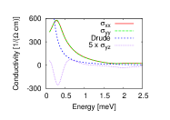
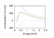
(a)	(b)
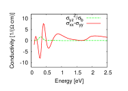
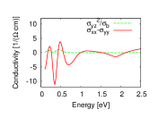
(c)	(d)

Figure 11: Conductivities $\sigma_{xx}$, $\sigma_{yy}=\sigma_{zz}$ and $\sigma_{yz}$ (magnetization along $\hat{x}$) corresponding to $p=1\ \mathrm{nm^{-3}}$ and $x=5\%$. (a) Real and (b) imaginary part of the interband conductivities according to Eq. (22), intraband (Drude) part is also shown. Note that the off-diagonal conductivity is magnified by a factor of $5$. (c/d) Real/imaginary part of the difference between diagonal components. The relatively small $(\mbox{Re }\sigma_{yz})^{2}/\sigma_{b}$ and $(\mbox{Im }\sigma_{yz})^{2}/\sigma_{b}$ with $\sigma_{b}=1500\ \mathrm{(\Omega\cdot cm)^{-1}}$ are also shown in panels (c) and (d).

Appendix D From conductivity to the Voigt effect in reflection

Typical $\sigma_{\parallel},\sigma_{\perp}$ as of Eq. (2) are shown in Fig. 11(a,b) (real and imaginary parts). Angle $\theta$ (and similarly $\psi$) is according to Eq. (15) related to their difference $\sigma_{\parallel}-\sigma_{\perp}$ and we therefore also plot this quantity. Some spectral features of Fig. 4a can be seen in Fig. 11c ($\mbox{Re }\sigma_{\parallel}-\sigma_{\perp}$) and Fig. 11d ($\mbox{Im }\sigma_{\parallel}-\sigma_{\perp}$) but their relationship is not straightforward.

Once the optical conductivities $\sigma_{\parallel}(\omega)$ and $\sigma_{\perp}(\omega)$ are known, effective permittivity and refractive indices can be calculated using Eq. (3)

$$n_{\parallel}^{2}=\mu\varepsilon_{\mathrm{eff}}^{\parallel}=\mu(\varepsilon_{b}+\frac{i\sigma_{||}}{\omega}),\qquad n_{\perp}^{2}\approx\mu\varepsilon_{\mathrm{eff}}^{\perp}=\mu(\varepsilon_{b}+\frac{i\sigma_{\perp}}{\omega})$$ (32)

where $\mu$ is the relative permeability which we take $\mu=1$. The $\varepsilon_{yz}^{2}/\varepsilon_{zz}$ term contributing to $n_{\perp}$ according to Eq. (14) can be neglected:not (c) diagonal components of permittivity are dominated by the background $\varepsilon_{b}$ and this large value causes $\sigma_{yz}/\sigma_{b}^{2}$ (with $\sigma_{b}=1500\ \mathrm{(\Omega\cdot cm)^{-1}}$ appropriate for $\varepsilon_{b}\approx 10.9$) to be small compared to $\sigma_{\parallel}-\sigma_{\perp}$ as shown in the lower panels of Fig. 11. Since both real and imaginary parts of $n_{\parallel}$ and $n_{\perp}$ differ, meaning that both (magnetic linear) birefringence and dichroism is present in our system, let us consider an illustrative example of how MLD and MLB individually influence the resultant $\theta$. Assume that $\varepsilon_{xx}=11.60+0.70i$ and $\varepsilon_{zz}=11.61+0.71i$; this is inspired by values in Fig. 11 and it would correspond to $\sigma\approx 100\ \mathrm{(\Omega\cdot cm)^{-1}}$ at $\hbar\omega=1$ eV and $|\sigma_{xx}-\sigma_{zz}|$ of the order of $1\ \mathrm{(\Omega\cdot cm)^{-1}}$. The rotation $\theta\approx\mbox{Re }\chi$, as given by Eq. (6), will be $0.151\ \mathrm{mrad}$ if reflection on an infinitely thick (Ga,Mn)As layer is considered, corresponding to Eq. (4). Now consider pure MLD situation: $\varepsilon_{xx}=11.60+0.70i$ and $\varepsilon_{zz}=11.60+0.71i$ would give $\theta=0.009\ \mathrm{mrad}$. On the other hand, $\varepsilon_{xx}=11.60+0.70i$ and $\varepsilon_{zz}=11.61+0.70i$ (pure MLB) results in $\theta=0.142\ \mathrm{mrad}$. It is clear that both MLD and MLB can significantly contribute to the spectra of rotation of the Voigt effect in reflection.

Taking into account the effect of the substrate as in Fig. 3 and Eq. (5) of Ref. Kim et al., 2007, (Ga,Mn)As refractive index $n$ leads to the reflection coefficient

$$r(n)=\frac{(n_{s}-1)\cos(kd)-i(n-n_{s}/n)\sin(kd)}{(n_{s}+1)\cos(kd)-i(n+n_{s}/n)\sin(kd)}.$$ (33)

Using Eqs. (32,33) we get $r(n_{\parallel})$ and $r(n_{\perp})$ that can be inserted into Eq. (5) and we finally obtain the rotation and ellipticity $\theta$, $\psi$. Multiple reflections in a (Ga,Mn)As layer are taken into account in Eq. (33), the complex $k=n\omega/c$, the layer has a finite thickness $d$ and it is sandwiched between vacuum and GaAs substrate with refractive indices $1$ and $n_{s}=\sqrt{\varepsilon_{b}+i\sigma_{\mathrm{GaAs}}/\omega\varepsilon_{0}}$, respectively. As it was explained below Eq. (3), we use $\omega$-dependent $\varepsilon_{b}$ which, together with intrinsic GaAs ac conductivity $\sigma_{\mathrm{GaAs}}(\omega)$ calculated from Eq. (22), reproduces experimentally known refractive index of GaAs. This seemingly over-cautious method of determining $n_{s}$ is important for maintaining the consistency of our optical model in Eq. (33). It guarantees that in the $x\to 0$, $p\to 0$ limit applied to our (Ga,Mn)As layer, reflection from the layer/substrate interface will be zero.

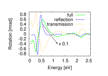
Figure 12: Rotation for a sample with $p=0.4\ \mathrm{nm^{-3}}$, $x=5\%$ and $d=20\ \mathrm{nm}$ in three situations: transmission (i.e. Voigt effect), reflection from a thick layer ($d\to\infty$) and geometry of our measurements (labelled ’full’). Note that the dashed curve is downscaled by a factor of 10 in the range $\hbar\omega<1.5\ \mathrm{eV}$.

Indeed, multilayer optical properties significantly influence the final form of the spectra (experimentally, thickness-dependence of $\theta$ at $\hbar\omega=1.58$ eV was studied by Al-Qadi et al. in Ref. Al-Qadi et al., 2012). Fig. 12 shows that differences between the transmission and reflection Voigt effect experiments could be significant, yet the spectral features (and their position in particular) remain to some extent unaffected. For example, peak $\alpha$ is somewhat suppressed in pure reflection (dashed curve in Fig. 12) that would correspond to an experiment with a thick layer ($d\to\infty$). Features $\beta$, $\gamma$ in the sub-gap energy range would, however, be order of magnitude larger in pure reflection. A hypothetical experiment measuring transmission (including multireflections) through a thin ($d=20\ \mathrm{nm}$) layer would give the Voigt effect as shown by the dotted curve where, roughly speaking, the spectrum only changes the overall sign. Multiple reflections between the substrate-sample and air-sample interfaces substantially modify the spectra although their effect may even be somewhat exaggerated in our model. Based on an estimate $\mbox{Re }\sigma_{xx}=\mbox{Im }\sigma_{xx}=200\ \mathrm{(\Omega\cdot cm)^{-1}}$ at $\hbar\omega=1\ \mathrm{eV}$ (compare Fig. 11), we obtain index of refraction $n\approx 1.2$ and therefore a large reflection coefficient at the substrate/sample interface. With absorption coefficients $\alpha(\omega)\sim 10000\ \mathrm{cm^{-1}}$, i.e. $\alpha d\approx 0.01\ll 1$, the wave will be (in our model) able to travel many times through the sample. Experimental comparison of the effect in samples with different thicknesses however suggests that both $\alpha d$ is larger and the sample/substrate contrast is lower ($n/n_{s}$ closer to one).

References

- Ferre and Gehring (1984) J. Ferre and G. A. Gehring, Rep. Prog. Phys. 47, 513 (1984).
- Jungwirth et al. (2006a) T. Jungwirth, J. Sinova, J. Mašek, J. Kučera, and A. H. MacDonald, Rev. Mod. Phys. 78, 809 (2006a).
- Burch et al. (2004) K. S. Burch, J. Stephens, R. K. Kawakami, D. D. Awschalom, and D. N. Basov, Phys. Rev. B 70, 205208 (2004).
- Kimel et al. (2005) A. V. Kimel, G. V. Astakhov, A. Kirilyuk, G. M. Schott, G. Karczewski, W. Ossau, G. Schmidt, L. W. Molenkamp, and T. Rasing, Phys. Rev. Lett. 94, 227203 (2005).
- Kim et al. (2007) M.-H. Kim, G. Acbas, M.-H. Yang, I. Ohkubo, H. Christen, D. Mandrus, M. A. Scarpulla, O. D. Dubon, Z. Schlesinger, P. Khalifah, et al., Phys. Rev. B 75, 214416 (2007).
- Acbas et al. (2009) G. Acbas, M.-H. Kim, M. Cukr, V. Novák, M. A. Scarpulla, O. D. Dubon, T. Jungwirth, J. Sinova, and J. Cerne, Phys. Rev. Lett. 103, 137201 (2009).
- Nagaosa et al. (2010) N. Nagaosa, J. Sinova, S. Onoda, A. H. MacDonald, and N. P. Ong, Rev. Mod. Phys. 82, 1539 (2010).
- (8) R. Schäfer and A. Hubert, phys. stat. sol. (a) 118, 271 (1990).
- Mertins et al. (2001) H.-C. Mertins, P. M. Oppeneer, J. Kuneš, A. Gaupp, D. Abramsohn, and F. Schäfers, Phys. Rev. Lett. 87, 047401 (2001).
- Kokado et al. (2012) S. Kokado, M. Tsunoda, K. Harigaya, and A. Sakuma, J. Phys. Soc. Jap. 81, 024705 (2012).
- Rushforth et al. (2007) A. W. Rushforth, K. Výborný, C. S. King, K. W. Edmonds, R. P. Campion, C. T. Foxon, J. Wunderlich, A. C. Irvine, P. Vašek, V. Novák, et al., Phys. Rev. Lett. 99, 147207 (2007).
- Kirilyuk et al. (2010) A. Kirilyuk, A. V. Kimel, and T. Rasing, Rev. Mod. Phys. 82, 2731 (2010).
- Kimel et al. (2004) A. V. Kimel, A. Kirilyuk, A. Tsvetkov, R. V. Pisarev, and T. Rasing, Nature 429, 850 (2004).
- Ando et al. (1998) K. Ando, T. Hayashi, M. Tanaka, and A. Twardowski, J. Appl. Phys. 83, 6548 (1998).
- Jungwirth et al. (2010) T. Jungwirth, P. Horodyská, N. Tesařová, P. Němec, J. Šubrt, P. Malý, P. Kužel, C. Kadlec, J. Mašek, I. Němec, et al., Phys. Rev. Lett. 105, 227201 (2010).
- Moore et al. (2003) G. P. Moore, J. Ferre, A. Mougin, M. Moreno, and L. Daweritz, J. Appl. Phys. 94, 4530 (2003).
- Tesařová et al. (2012) N. Tesařová, J. Šubrt, P. Malý, P. Němec, C. T. Ellis, A. Mukherjee, and J. Cerne, Rev. Sci. Inst. 83, 123108 (2012).
- Abolfath et al. (2001) M. Abolfath, T. Jungwirth, J. Brum, and A. H. MacDonald, Phys. Rev. B 63, 054418 (2001).
- Ebert (1996) H. Ebert, Rep. Prog. Phys. 59, 1665 (1996).
- not (a) Cyclotron resonance (in non-magnetic materials) gives rise to a peak in absorption which shifts with increasing magnetic field.Orlita et al. (2013) The term ”magnetooptics” also commonly embraces this effect.
- Orlita et al. (2013) M. Orlita, W. Escoffier, P. Plochocka, B. Raquet, and U. Zeitler, Comptes Rendus Physique 14, 78 (2013).
- Buchmeier et al. (2009) M. Buchmeier, R. Schreiber, D. E. Bürgler, and C. M. Schneider, Phys. Rev. B 79, 064402 (2009).
- not (b) Hubert and SchäferSchafer:1990_a (HS) observed an effect related to magnetization gradient while studying in-plane magnetized domains of magnetic thin films. It was later named the HS effectKamberský (1992) but since the original reference Schafer:1990_a also reports on the observation of the Voigt effect in reflection, terminology became somewhat confused. Boundary effects in systems with magnetic domains (and non-zero magnetic gradients) naturally receive the name HS effectBanno (2008) but x-ray Voigt effect in reflection off thin iron layers with homogeneous magnetization has also been called HS effect.Valencia et al. (2010) In the present article, we adhere to the original conventionSchafer:1990_a and use the term ”Voigt effect in reflection”.
- Kamberský (1992) V. Kamberský, J. Magn. Magn. Mat. 104–107, 311 (1992).
- Banno (2008) I. Banno, Phys. Rev. A 77, 033818 (2008).
- Valencia et al. (2010) S. Valencia, A. Kleibert, A. Gaupp, J. Rusz, D. Legut, J. Bansmann, W. Gudat, and P. M. Oppeneer, Phys. Rev. Lett. 104, 187401 (2010).
- Postava et al. (1997) K. Postava, H. Jaffres, A. Schuhl, F. N. V. Dau, M. Goiran, and A. Fert, J. Magn. Magn. Mat. 172, 199 (1997).
- Nemec et al. (2013) P. Němec, V. Novák, N. Tesařová, E. Rozkotová, H. Reichlová, D. Butkovičová, F. Trojánek, K. Olejník, P. Malý, R. P. Campion, et al., Nat. Commun. 4, 1422 (2013).
- Zemen et al. (2009) J. Zemen, J. Kucera, K. Olejnik, and T. Jungwirth, Phys. Rev. B 80.
- Kim et al. (2011) M.-H. Kim, V. Kurz, G. Acbas, C. T. Ellis, and J. Cerne, J. Opt. Soc. Am. B 28, 199 (2011).
- Sato (1981) K. Sato, Jpn. J. Appl. Phys. 20, 2403 (1981).
- Tesarova et al. (2012) N. Tesařová, P. Němec, E. Rozkotová, J. Šubrt, H. Reichlová, D. Butkovičová, F. Trojánek, P. Malý, V. Novák, and T. Jungwirth, Appl. Phys. Lett. 100, 102403 (2012).
- Hamrle et al. (2007) J. Hamrle, S. Blomeier, O. Gaier, B. Hillebrands, H. Schneider, G. Jakob, K. Postava, and C. Felser, J. Phys. D: Appl. Phys. 40, 1563 (2007).
- Oh et al. (1991) E. Oh, D. U. Bartholomew, A. K. Ramdas, J. K. Furdyna, and U. Debska, Phys. Rev. B 44, 10551 (1991).
- Jancu et al. (1998) J.-M. Jancu, R. Scholz, F. Beltram, and F. Bassani, Phys. Rev. B 57, 6493 (1998).
- Bebb (1969) H. B. Bebb, Phys. Rev. 185, 1116 (1969).
- Chapler et al. (2013) B. C. Chapler, S. Mack, R. C. Myers, A. Frenzel, B. C. Pursley, K. S. Burch, A. M. Dattelbaum, N. Samarth, D. D. Awschalom, and D. N. Basov, Phys. Rev. B 87, 205314 (2013).
- Dietl et al. (2000) T. Dietl, H. Ohno, F. Matsukura, J. Cibert, and D. Ferrand, Science 287, 1019 (2000).
- not (c) Appendix D discusses the smallness of from theoretical point of view. Alternatively, data in Ref. Acbas et al., 2009 (Fig. 1a, rad/cm) imply using Eq. (13) of Ref. Kim et al., 2007 . This translates to (relative) at eV, hence (for ). This is small compared to (see Appendix D).
- Lautenschlager et al. (1987) P. Lautenschlager, M. Garriga, S. Logothetidis, and M. Cardona, Phys. Rev. B 35, 9174 (1987).
- Johnson et al. (1969) C. J. Johnson, G. H. Sherman, and R. Weil, Appl. Opt. 8, 1667 (1969).
- da Silva et al. (2004) J. H. D. da Silva, R. R. Campomanes, D. M. G. Leite, F. Orapunt, and S. K. O’Leary, J. Appl. Phys. 96, 7052 (2004).
- Tauc et al. (1966) J. Tauc, R. Grigorovici, and A. Vancu, physica status solidi (b) 15, 627 (1966).
- not (d) Comparing (Ga,Mn)As to amorphous GaAs, it should be mentioned that chemical rather than structural disorder has also other ramifications than the inapplicability of Bloch theorem. The hybridization between -like orbitals of GaAs with -like Mn orbitals of course does change the orbital character of the valence band to some extent, so that the matrix elements in Eq. (22) will be modified. In particular, the parameter mentioned above Eq. (20) will bear witness to the modified orbitals through and optical transition probabilities will naturally also be modified. This effect is ”hidden” behind the Schrieffer-Wolff transformation included in the model of Ref. Abolfath et al., 2001. Consequently, heights of the peaks in will change.
- Jungwirth et al. (2007) T. Jungwirth, J. Sinova, A. H. MacDonald, B. L. Gallagher, V. Novák, K. W. Edmonds, A. W. Rushforth, R. P. Campion, C. T. Foxon, L. Eaves, et al., Phys. Rev. B 76, 125206 (2007).
- Moss (1954) T. S. Moss, Proceedings of the Physical Society. Section B 67, 775 (1954).
- not (e) Exchange energy as we describe it can lead to Bloch ferromagnetism at low electron densities as it is very clearly explained in Sec. II of Ref. Zhang:2005_c, ). This transition results from the competition of the exchange energy with kinetic energy. At higher densities relevant for our system, the former does not exceed the latter so that the ferromagnetic state would not appear were it not for the additional interaction with manganese magnetic moments. However, since the exchange energy grows relative to with increasing carrier density, it may be important to our considerations here.
- (48) Y. Zhang and S. Das Sarma, Phys. Rev. B 72, 115317 (2005).
- Sipahi et al. (1996) G. M. Sipahi, R. Enderlein, L. M. R. Scolfaro, and J. R. Leite, Phys. Rev. B 53, 9930 (1996).
- Zhang and Das Sarma (2005) Y. Zhang and S. Das Sarma, Phys. Rev. B 72, 125303 (2005).
- Yang et al. (2003) S.-R. E. Yang, J. Sinova, T. Jungwirth, Y. P. Shim, and A. H. MacDonald, Phys. Rev. B 67, 045205 (2003).
- Osgood III et al. (1998) R. Osgood III, S. Bader, B. Clemens, R. White, and H. Matsuyama, J. Magn. Magn. Mat. 182, 297 (1998).
- not (f) A derivation based on the analogy between and is given in Ref. Osgood III et al., 1998.
- not (g) Onsager relations imply . For , follows from applying mirror inversion with respect to the plane to .
- Birss (1964) R. R. Birss, Symmetry and magnetism (North-Holland Publishing Company, Amsterdam, 1964).
- Višňovský (1986) Š. Višňovský, Czech. J. Phys. B 36, 1424 (1986).
- Postava et al. (2002) K. Postava, D. Hrabovsky, J. Pistora, A. R. Fert, S. Visnovsky, and T. Yamaguchi, J. Appl. Phys. 91, 7293 (2002).
- Bhagavantam (1966) S. Bhagavantam, Crystal symmetry and physical properties (Academic Press, London and New York, 1966).
- Hamrlová et al. (2013) J. Hamrlová, J. Hamrle, K. Postava, and J. Pištora, phys. stat. sol. (b), published on-line (2013), doi: 10.1002/pssb.201349031.
- de Ranieri et al. (2008) E. de Ranieri, A. W. Rushforth, K. Výborný, U. Rana, E. Ahmad, R. P. Campion, C. T. Foxon, B. L. Gallagher, A. C. Irvine, J. Wunderlich, et al., New J. Phys. 10, 065003 (2008).
- Piano et al. (2011) S. Piano, R. Grein, C. J. Mellor, K. Výborný, R. Campion, M. Wang, M. Eschrig, and B. L. Gallagher, Phys. Rev. B 83, 081305 (2011).
- Jungwirth et al. (2006b) T. Jungwirth, J. Mašek, K. Y. Wang, K. W. Edmonds, M. Sawicki, M. Polini, J. Sinova, A. H. MacDonald, R. P. Campion, L. X. Zhao, et al., Phys. Rev. B 73, 165205 (2006b).
- Hankiewicz et al. (2004) E. M. Hankiewicz, T. Jungwirth, T. Dietl, C. Timm, and J. Sinova, Phys. Rev. B 70, 245211 (2004).
- Kolorenč et al. (2002) J. Kolorenč, L. Smrčka, and P. Středa, Phys. Rev. B 66, 085301 (2002).
- Allen (2006) P. Allen, in Conceptual Foundations of Materials A Standard Model for Ground- and Excited-State Properties, edited by S. G. Louie and M. L. Cohen (Elsevier, 2006), vol. 2 of Contemporary Concepts of Condensed Matter Science, pp. 165 – 218.
- not (h) The standard way to microscopically link to potential disorder is to include potential of randomly positioned impurities into and average over the positions. This procedure is explained in Sec. 8.1.2 of G. Mahan, Many-Particle physics (Kluwer Academic/Plenum Publishers, New York, 2000, third edition). Alternatively, can also be introduced as inverse relaxation time when the electron is weakly interacting with its surroundings.Lax (1958)
- Lax (1958) M. Lax, Phys. Rev. 109, 1921 (1958).
- Al-Qadi et al. (2012) B. Al-Qadi, N. Nishizawa, K. Nishibayashi, M. Kaneko, and H. Munekata, Applied Physics Letters 100, 222410 (pages 4) (2012).