Numerical approach to unbiased and driven generalized elastic model

Abstract

From scaling arguments and numerical simulations, we investigate the properties of the generalized elastic model (GEM), that is used to describe various physical systems such as polymers, membranes, single-file systems, or rough interfaces. We compare analytical and numerical results for the subdiffusion exponent $\beta$ characterizing the growth of the mean squared displacement $\langle(\delta h)^{2}\rangle$ of the field $h$ described by the GEM dynamic equation. We study the scaling properties of the $q$th order moments $\langle|\delta h|^{q}\rangle$ with time, finding that the interface fluctuations show no intermittent behavior. We also investigate the ergodic properties of the process $h$ in terms of the ergodicity breaking parameter and the distribution of the time averaged mean squared displacement. Finally, we study numerically the driven GEM with a constant, localized perturbation and extract the characteristics of the average drift for a tagged probe.

I Introduction

In the past two decades, considerable theoretical and numerical effort has been put into the characterization and quantitative modeling of stochastic patterns such as surface growth processes surface1 ; surface2 , spatiodynamic profiles of elastic chains granek1997 , single-file systems single , membranes zilman2002 ; helfer2000 , and polymers doi ; amblard1996 ; everaers1999 ; caspi1998 , as well as fluid interface motion through porous media buldyrev1992 ; nissen2001 , the shape of vortex lines in high $T_{c}$ superconductors bustingorry2006 , tumor growth bru1998 , and crack propagation podlubny . For obvious reasons, these processes are of substantial interest both from a fundamental physics and technological applications point of view. To obtain a quantitative understanding, different continuum models have been proposed and studied to reproduce the dynamics of such natural phenomena. The simplest and well-known examples are the Edwards-Wilkinson and the Mullins-Herring equations surface1 ; surface2 . Such models provide information about the out-of-equilibrium dynamics of the field $h(\mathbf{x},t)$, that describes the height profile of the surface under consideration, a membrane, etc. For processes such as the spatiotemporal evolution of a polymer configuration, $h$ becomes a vector field. In what follows, we concentrate on scalar fields $h$ and its governing diffusion-noise equation vankampen .

The generalized elastic model (GEM) proposed and analyzed in Refs. taloni2010 ; taloni2012 ; taloni2011 ; taloni2013 unifies various classes of stochastic processes such as the configuration dynamics of semiflexible, flexible, and Rouse polymers, fluid membranes, single-file system, fluctuating interfaces, solid surfaces, and the diffusion-noise equation. Suppose you follow the dynamics of a particular tracer particle in a stochastic system described by the field $h(\mathbf{x},t)$. This could be a labeled lipid molecule in a membrane or an individual particle in a single-file system. The motion of such a tracer particle is then necessarily coupled to the rest of the system, and this correlated dynamics effects the subdiffusive motion of the tracer particle, characterized by the subdiffusion exponent $\beta$ in the mean squared displacement of the field $h$ with time,

$$\langle(\delta h)^{2}\rangle\simeq t^{2\beta},$$ (1)

with $0<\beta<1/2$ REM The dynamic exponent $\beta$ is but one of three scaling exponents characteristic for stochastic processes described by the GEM, the other two being the roughness exponent $\xi$ and the dynamic exponent $\nu$. The triple of these exponents are most commonly used to classify surface growth dynamics surface1 ; surface2 . Here we investigate numerically the scaling properties of the GEM, in particular, we obtain the dynamic exponent $\tau(q,\beta)$ of the general $q$th order moments $\langle|\delta h|^{q}\rangle\simeq t^{\tau(q,\beta)}$.

Starting from early studies of the long-time out-of-equilibrium dynamics of glassy materials struik1978 , many complex systems characterized by anomalous diffusion bouchaud ; report were shown to exhibit ageing effects and weak ergodicity breaking bouchaud1992 ; cugliandolo1995 ; monthus1996 ; rinn2000 ; barkai2003 ; bel2005 ; rebenshtok2007 ; johannes . Respectively, these effects refer to the dependence of the dynamics of such system on their age since the initial preparation, and the fact that long time and ensemble averaged observables behave differently and are irreproducible. In particular, important consequences of such weak ergodicity breaking were studied in the non-stationary continuous time random walk (CTRW) model and used to interpret single molecule tracking data He2008 ; burov2011 ; Joen2011 . Similar weak ergodicity breaking is observed for regular diffusion equation dynamics with space-dependent diffusion coefficient and explicitly aging CTRW processes cherstvy2013 ; lomholt . Closely related to the GEM, other anomalous diffusion systems such as fractional Brownian motion and fractional Langevin equation motion are ergodic deng2009 , but exhibit transient aging and weak ergodicity breaking jochen . As originally pointed out by Taloni et al. taloni2012 , time and ensemble averages of the squared displacement of a tracer particle in the GEM with non-equilibrium initial conditions are disparate. In the present paper we study numerically the ergodic properties of the GEM by probing quantities such as the amplitude scatter of time averaged observables and the ergodicity breaking parameter EB.

In order to further characterize the viscoelastic properties of the system under study, we also consider the case of a driven GEM, that is, the response of the GEM dynamics to an external localized force, supposed to act only on a single tagged probe taloni2011 . Below we analyze the driven GEM numerically in order to investigate the motion of this tagged probe.

The paper is organized as follows: in Section II we introduce the notation and define the GEM and the GEM with localized perturbation. In Section III we report a general method to simulate the GEM numerically. The numerical results are discussed in Section IV. Finally, we draw our Conclusions in Section V. To be self-explanatory we add two Appendices to explain efficient ways to approximate the space fractional operator and to generate fractional Gaussian noise.

II Definitions and settings

The GEM is defined in terms of the stochastic linear partial integrodifferential equation taloni2010

$$\frac{\partial}{\partial t}h(\mathbf{x},t)=\int d^{d}x^{\prime}\Lambda(|\mathbf{x}-\mathbf{x}^{\prime}|)\frac{\partial^{z}}{\partial|\mathbf{x}^{\prime}|^{z}}h(\mathbf{x}^{\prime},t)+\eta(\mathbf{x},t)~{},$$ (2)

where the scalar field $h(\mathbf{x},t)$ is parameterized by the coordinate $\mathbf{x}$ and time $t$. The integral kernel $\Lambda(|\mathbf{x}-\mathbf{x}^{\prime}|)$ of the spatial convolution integral represents the generally non-local coupling of different sites $\mathbf{x}$ and $\mathbf{x}^{\prime}$. Moreover, $\partial^{z}/\partial|\mathbf{x}|^{z}$ is the multidimensional Riesz-Feller fractional space derivative of order $z$ which is defined via its Fourier transform through the functional relation samko

$$\mathscr{F}\left\{\frac{\partial^{z}}{\partial|\mathbf{x}|^{z}}h(\mathbf{x},t)\right\}\equiv-|\mathbf{q}|^{z}h(\mathbf{q},t).$$ (3)

Here, $h(\mathbf{q},t)$ is the Fourier transform of $h(\mathbf{q},t)$. The Gaussian noise $\eta(\mathbf{x},t)$ is fully determined by its first two moments, $\langle\eta(\mathbf{x},t)\rangle=0$ and

$$\langle\eta(\mathbf{x},t)\eta(\mathbf{x}^{\prime},t^{\prime})\rangle=2k_{B}T\Lambda^{\prime}(|\mathbf{x}-\mathbf{x}^{\prime}|)\delta(t-t^{\prime}),$$ (4)

where $\Lambda^{\prime}(r)$ with $r=|\mathbf{x}-\mathbf{x}^{\prime}|$ represents spatial correlation properties of the noise.

It is important to note that, in general, $\Lambda(r)\neq\Lambda^{\prime}(r)$, that is, both functions may be chosen independently. In what follows, to extract the scaling properties of the GEM we first consider the general situation with long ranged hydrodynamic-style interactions, $\Lambda(r)\sim r^{-\alpha_{1}}$, and fractional Gaussian noise with long range spatial correlations, $\Lambda^{\prime}(r)\sim r^{-\alpha_{2}}$. We will discuss the following special cases:

(a) The interaction is local, $\Lambda(r)=\delta(r)$, and the noise is an uncorrelated Gaussian random variable, $\Lambda^{\prime}(r)=\delta(r)$. This special case corresponds to taking $\alpha_{1}=\alpha_{2}=d$.

(b) The interaction term $\Lambda$ is non-local with long-range power-law interaction and the random noise $\eta$ has long-range correlations, both with the same exponents $\alpha_{1}=\alpha_{2}=\alpha$.

(c) The interaction is local, $\Lambda(r)=\delta(r)$ ($\alpha_{1}=d$), and the noise is long-range correlated, $\Lambda^{\prime}(r)\propto r^{-\alpha}$ ($\alpha_{2}=\alpha$).

(d) The interaction is non-local, $\Lambda(r)\propto r^{-\alpha}$ ($\alpha_{1}=\alpha$), and the noise is uncorrelated and Gaussian, $\Lambda^{\prime}(r)=\delta(r)$ ($\alpha_{2}=d$).

In cases (a) and (b) the fluctuation-dissipation relation of the second kind holds, whereas in cases (c) and (d) it is violated. In the latter case the noise would then be viewed to be external. The properties of the GEM in the presence of the fluctuation-dissipation theorem have been studied analytically by Taloni et al. taloni2010 ; taloni2012 ; taloni2011 ; taloni2013 . It is worthwhile mentioning that $z=2$ in case (a) corresponds to the Edwards-Wilkinson equation, and $z=4$ describes the universality class of the Mullins-Herring equation surface1 ; surface2 . The Edwards-Wilkinson and Mullins-Herring equations with long-range correlated power-law noise [cases (a) and (c)] were studied in Ref. yu1994 ; pang1997 ; pang2010 . Krug et al. krug1997 used Eq. (2) with local interaction $\Lambda(r)=\delta(r)$ to study the first passage statistics of locally fluctuating interfaces. There Eq. (2) was solved numerically for the special cases $z=2$ and $4$. Majumdar et al. majumdar considered the same model to study the first-passage properties in space.

Bearing in mind certain physical situations such as a cytoskeletal filament pushing a single lipid in a vicinal membrane with some force taloni2011 , it will be interesting to consider the influence of such localized perturbations. To that end we consider the extended GME equation

$$\frac{\partial}{\partial t}{h}\left(\mathbf{x},t\right) = \int d^{d}x^{\prime}\Lambda\left(\mathbf{x}-\mathbf{x}^{\prime}\right)$$ (5)

$$\times\left[\frac{\partial^{z}}{\partial|\mathbf{x}^{\prime}|^{z}}{h}(\mathbf{x}^{\prime},t)+\mathbf{F}\left\{h(\mathbf{x}^{\prime},t),t\right\}\delta(\mathbf{x}^{\prime}-\mathbf{x}^{\star})\right]$$

$$+\eta\left(\mathbf{x},t\right),$$

such that the external force $\mathbf{F}$ acts only on the single (tagged) probe at position $x^{\star}$ taloni2011 . This local force breaks the translational invariance of the problem. We are interested in measuring the average drift $\langle h(x^{\star},t)\rangle_{F_{0}}$ in the perturbed system with the constant force $\mathbf{F}\{h(x^{\prime},t),t\}=F_{0}\Theta(t)$ for different types of the GEM. The forced problem will be discussed in Section IV.4.

III The GEM on a lattice

To solve Eqs. (2) and (5) numerically, we convert the dynamic formulation to discrete time and space in $d=1$. To that end we define $t=n\Delta t$ with $n=1,2,\dots,N$ and $x=i\Delta x$ with $i=-L/2,\dots,L/2$, where $\Delta t$ and $\Delta x$ are the grid steps in time and space, respectively. To approximate the time derivative one can use a simple forward Euler differential scheme,

$$\frac{\partial h(x_{i},t_{n})}{\partial t}=\frac{h(x_{i},t_{n+1})-h(x_{i},t_{n})}{\Delta t}.$$ (6)

In the following two Subsections, we review the methods to obtain a discrete version of the fractional operator $\partial^{z}/\partial|x|^{z}$ and to generate the correlated noise $\eta(x,t)$ with long-range correlation $\Lambda^{\prime}(r)\sim r^{-\alpha}$. Then, we use the discrete version of Eqs. (2) and (5) in our numerical simulations.

III.1 The discretized fractional operator

Rewriting the integral term of the GMEs (2) and (5) with a power-law kernel $\Lambda(r)$ in terms of a space-fractional differential expression allows us to use known numerical methods for analysis. Indeed the concept of fractional operators has been successfully applied to a wide field of problems in physics, chemistry, finance, biology and hydrology report ; samko ; podlubny ; kilbas . Here we employ the discrete-space representation of the Riesz-Feller derivative $\partial^{z}/\partial|x|^{z}$ of fractional order $z$. Different numerical methods have been proposed to simulate such fractional operators yang . We here pursue the following approach. We rewrite the Riesz-Feller derivative in terms of the standard Laplacian $\Delta^{2}$ as $\partial^{z}/\partial|x|^{z}:=-(-\Delta)^{z/2}$ saichev1997 , and then use the matrix transform method proposed by Ilić et al ilic2005 to approximate the discrete space fractional operator (see also Appendix A).

Let us first consider the usual Laplacian in one dimension and a complete set of orthogonal functions $\{\phi(x)\}$. In terms of the finite difference method,

$$\Delta\phi(x)=\frac{\phi(x-a)-2\phi(x)+\phi(x+a)}{a^{2}},$$ (7)

where $a$ represents the lattice constant. With the Fourier representation

$$\phi(x)=\frac{1}{2\pi}\int\widehat{\phi}(q)e^{-iqx}dq,$$ (8)

we obtain the Fourier transform of the discretized Laplacian Eq. (7) as

$$\widehat{(\Delta)}\phi(q)=-[2-2\cos(qa)]\phi(q).$$ (9)

On the other hand one can find the elements of the matrix representation of the Laplacian,

$$\mathbb{A}_{l,m}=-\int_{0}^{2\pi}\frac{dq}{2\pi}[2-2\cos(qa)]e^{iq(l-m)},$$ (10)

where the tridiagonal matrix $\mathbb{A}\equiv\text{tridiag}(1,-2,1)$ has nonzero elements only in the main diagonal and the first diagonals below and above the main one.

We now use the approximation proposed by Ilić et al (compare also Appendix A and Refs. ilic2005 ; yang ) to find the Fourier representation of the fractional Laplacian. Namely, we start with the Fourier representation of the discretized Laplacian $(-\Delta)$ with the minus sign, $\lambda(q)=2[1-\cos(q)]$ and raise it to the appropriate power, $(2[1-\cos(q)])^{z/2}$ zoia2007 . Here the lattice constant has been set equal to one. The elements of the matrix $\mathbb{K}$, representing the discretized fractional Laplacian $-(-\Delta)^{z/2}$ are then given by

$$\mathbb{K}_{l,m} = -\int_{0}^{2\pi}\frac{dq}{2\pi}e^{iq(l-m)}\Big{(}2[1-\cos(q)]\Big{)}^{z/2}$$ (11)

$$= \frac{\Gamma(-z/2+n)\Gamma(z+1)}{\pi\Gamma(1+z/2+n)}\sin\left(\frac{z}{2}\pi\right),$$

where $n=|l-m|$, and the fractional order $z\geq 1$. In the special case $z=2$ the $\mathbb{K}$ matrix is equal to the matrix $\mathbb{A}$ of the regular Laplacian. Moreover, if $\alpha/2$ is an integer, then $\mathbb{K}(n)=(-1)^{\alpha-n+1}C_{\alpha,n+\alpha/2}$ for $n\leq\alpha/2$ and $\mathbb{K}(n)=0$ for $n>\alpha/2$, where the $C_{\alpha,n+\alpha/2}$ represent binomial coefficients zoia2007 .

III.2 Fractional Gaussian noise

Several methods have been used to generate one-dimensional random processes with long-range correlations, for instance, the successive random addition method peitgen , the Weierstrass-Mandelbrot function ausloos1985 as well as the optimization method hamzehpour2006 . A very efficient way to generate fractional Gaussian noise (fGn) is the modified Fourier filtering (MFF) method makse1996 , compare also Appendix B.

Following Ref. makse1996 , one needs a slightly modified correlation function to deal with the singularity of $\Lambda^{\prime}(r)$ at $r=0$ and to generate the correlated noise. We use the form

$$\Lambda^{\prime}_{c}(r)=(c^{2}+r^{2})^{-\alpha/2},$$ (12)

with the asymptotically correct behavior $\Lambda^{\prime}_{c}(r)\sim r^{-\alpha}$ at $r\gg c$. The continuum limit of the spectral density $\Lambda^{\prime}_{c}(q)$ becomes

$$\Lambda^{\prime}_{c}(q)\equiv\mathscr{F}\left\{\Lambda^{\prime}_{c}(r)\right\}=\frac{\sqrt{\pi}2^{1-\gamma}c^{-\gamma}}{\Gamma(\alpha/2)}|q|^{\gamma}K_{\gamma}(c|q|),$$ (13)

where $\gamma=(\alpha-1)/2$ and $K_{\gamma}$ is the modified Bessel function of order $\gamma$. Then for small values of $c$ and $q$, Eq. (13) leads to the asymptotic behavior $\Lambda^{\prime}_{c}(q)\sim q^{\alpha-1}$ (see Eq. (36)).

The numerical algorithm for generating correlated noise $\eta$ for arbitrary values of $\alpha$ consists of the following steps:

(i.) Generate a one-dimensional array of uncorrelated Gaussian random variables, $w_{i}$, and compute their Fourier transform $w_{q}$.

(ii.) Calculate $\{\eta(q,t_{n})\}=\left[\Lambda_{c}^{\prime}(q)\right]^{1/2}w_{q}$, where $\Lambda_{c}^{\prime}(q)$ is given by Eq. (13).

(iii.) Calculate the inverse Fourier transform $\eta(x_{i},t_{n})=\mathscr{F}^{-1}\{\eta(q,t_{n})\}$ to obtain the correlated noise with the desired correlation exponent $\alpha$ in the real space.

We should note that we use periodic boundary condition, i.e., $\Lambda^{\prime}_{c}(r)=\Lambda^{\prime}_{c}(r+L)$ in the interval $[-L/2,\dots,L/2]$, consequently we get the correlated sample with the same periodicity. It is also possible to generate a sample with natural boundary conditions. To this end, one first needs to generate a sample with periodic boundary condition, of size $2L$, and then cuts the sequences of the fGn time series into two separate parts with the same size $L$, where each part obeys an open boundary condition.

For the uncorrelated case $\Lambda^{\prime}(r)=\delta(r)$, the noise $\eta$ has a Gaussian distribution and every $\eta(x_{i},t_{n})$ is an independent random variable with zero mean and unit variance [with the convention $k_{B}T=1$ in Eq. (4)].

With these definitions we represent Eqs. (2) and (5) in terms of discrete space and time variables $x_{i}=i\Delta x$ and $t_{n}=n\Delta t$ in the form

$$h_{i}^{n+1} = h_{i}^{n}+\Delta t\sum_{j=-L/2}^{L/2}\sum_{k=-L/2}^{L/2}\Lambda(|i-j|)\mathbb{K}_{j,k}h_{k}^{n}$$ (14)

$$+\sqrt{2\Delta t}\eta_{i}^{n},$$

where $h_{i}^{n}$ approximates the field $h(x_{i},t_{n})$ at the $i$th lattice point and the $n$th time step. At any given time step $n$, one needs to generate the random process $\eta_{i}^{n}$ with the appropriate correlation function $\Lambda^{\prime}$. Analogously, the lattice version of the driven GEM with localized perturbation becomes

$$h_{i}^{n+1} = h_{i}^{n}+\Delta t\sum_{j=-L/2}^{L/2}\sum_{k=-L/2}^{L/2}\Lambda(|i-j|)\mathbb{K}_{j,k}h_{k}^{n}$$ (15)

$$+\Delta t\Lambda(|i-i^{\star}|)\mathbf{F}\{h(i^{\star},n),n\}+\sqrt{2\Delta t}\eta_{i}^{n},$$

where $i^{\star}$ corresponds to the position of the tagged probe. In the next Section we present our numerical results and compare them with the analytical predictions.

IV Results

To determine the time evolution of the scalar field $h(x,t)$ and to obtain the dynamic scaling properties of the GEM, we simulated this model on a lattice of size $L=4098$. All simulation measurements are based on an ensemble of $500$ realizations. In the simulations the time increment $\Delta t$ should be small enough to ensure the stability of the numerical algorithm, and we find that $\Delta t=0.05$ is a good working choice. As offset for $\Lambda^{\prime}_{c}$ we choose $c=0.05$. As already mentioned above, in order to avoid finite size effects we impose periodic boundary conditions. At first we consider the unbiased discrete GEM (14) with non-thermal initial condition [$h(i,0)=0$, $i\in[-L/2,\dots,L/2]$], and we measure the scaling exponents $\beta$ and $\tau(q,\beta)$ of the second and $q$th order moments. Then we test the ergodic properties of the GEM with non-thermal initial condition. Finally, we move to the lattice version of the driven GEM (15) with localized perturbation and measure the average drift for the tagged probe.

IV.1 Scaling laws and the $h$-correlation function

The solution of the GEM (2) has a continuous scale invariance property, that is, for a physical observable $\mathcal{O}$ the relation

$$\mathcal{O}(\lambda\mathbf{x},\lambda^{\nu}t)=\mu(\lambda)\mathcal{O}(\mathbf{x},t)$$ (16)

arises, where $\mu(\lambda)$ is a power function of the scale factor $\lambda$. This means that Eq. (2) does not change under a scaling transformation $\mathbf{x}\rightarrow\lambda\mathbf{x}$ and $t\rightarrow\lambda^{\nu}t$, together with the corresponding rescaling in the amplitude, $h\rightarrow\lambda^{\xi}h$.

The scaling properties of the stochastic field $h(\mathbf{x},t)$ in a $d$-dimensional space of linear size $L$ can be also characterized in terms of the global interface width $W(t)$ defined by the root-mean-square fluctuation of the random profile $h(x,t)$ at site $x$ and time $t$, that is,

$$W(t)=\left<\int dx[h(\mathbf{x},t)-\langle h(t)\rangle]^{2}\right>^{1/2},$$ (17)

where $\langle h(t)\rangle=\int d^{d}xh(\mathbf{x},t)$. This width $W(t)$ scales as

$$W(t)\sim L^{\xi}f(t/L^{\nu})\sim\left\{\begin{array}[]{ll}t^{\beta},&t\ll t_{s}\\[5.69046pt] L^{\xi},&t\gg t_{s}\end{array}\right.,$$ (18)

where $t_{s}=L^{\nu}$ is the so-called saturation time and $f(x)$ is a scaling function with the property $f(x)\sim x^{\beta}$ for $x\ll 1$ and $f(x)\sim const.$ for $x\gg 1$ surface1 ; surface2 . According to Eq. (18), we obtain the constraint $\beta=\xi/\nu$ between the scaling exponents. With these relations we obtain the scaling exponents $\xi$, $\nu$, and $\beta$ for different forms of the interaction kernel $\Lambda$ and the noise correlation function $\Lambda^{\prime}$. To this end we consider $\Lambda(r)\sim r^{-\alpha_{1}}$ and $\Lambda^{\prime}(r)\sim r^{-\alpha_{2}}$. If $\alpha_{1}=d$, the hydrodynamic interaction is local, while $\alpha_{2}=d$ corresponds to a system with uncorrelated thermal noise. The scale transformations $\mathbf{x}\rightarrow\lambda\mathbf{x}$ and $t\rightarrow\lambda^{\nu}t$ transform the GEM (2) according to

$$\frac{\partial}{\partial t}h(\mathbf{x},t) = \lambda^{\nu-\gamma}\int d^{d}x^{\prime}\Lambda(\mathbf{x}-\mathbf{x}^{\prime})\frac{\partial^{z}}{\partial|\mathbf{x}^{\prime}|^{z}}h(\mathbf{x}^{\prime},t)$$ (19)

$$+\lambda^{(\nu-\alpha_{2})/2-\xi}\eta(\mathbf{x},t),$$

where $\gamma=z+\alpha_{1}-1$. The scale-invariance of the solution of the GEM (2) implies that $\nu=z+\alpha_{1}-d$ and $\xi=(z+\alpha_{1}-\alpha_{2}-d)/2$. This specifies the dynamic scaling exponent

$$\beta=\frac{(z+\alpha_{1}-\alpha_{2}-d)}{2(z+\alpha_{1}-d)}.$$ (20)

We now turn to determine the scaling properties of the $h$-correlation function for the GEM with general interaction kernel $\Lambda(r)\sim r^{-\alpha_{1}}$ and noise correlation $\Lambda^{\prime}(r)\sim r^{-\alpha_{2}}$. Some previous measures of the $h$-correlation for the special cases with $\alpha_{1}=\alpha_{2}=d$ [our case (a)] and $\alpha_{1}=\alpha_{2}=\alpha$ [our case (b)] were studied in Refs. taloni2010 ; taloni2012 ; taloni2013 .

To derive the $h$-correlation function for the GEM with general interaction kernel $\Lambda(r)$ and noise correlation $\Lambda^{\prime}(r)$ we follow the method put forward in Ref. taloni2012 . We first consider the flat initial condition $h(x,0)=0$, the so-called non-thermal initial condition taloni2012 ; krug1997 . We mention that the dynamics of the GEM depends on the specific choice of the initial condition of Eq. (2), compare the discussion in Ref. taloni2012 . Then, the one-point, two-time correlation function reads

$$\langle\delta_{t}h(\mathbf{x},t)\delta_{t^{\prime}}h(\mathbf{x},t^{\prime})\rangle = \langle[h(\mathbf{x},t)-h(\mathbf{x},0)]$$ (21)

$$\times[h(\mathbf{x},t^{\prime})-h(\mathbf{x},0)]\rangle$$

$$=K\left[(t+t^{\prime})^{2\beta}-|t-t^{\prime}|^{2\beta}\right],$$

where $\beta$ matches the result of our above scaling arguments, compare Eq. (20), and we find

$$K=\frac{2k_{B}T\pi^{d/2}}{(2\pi)^{d}\Gamma(d/2)}\frac{\Gamma(1-2\beta)}{z-d}\left(\frac{(4\pi)^{d/2}}{2^{\alpha}}\frac{\Gamma((d-\alpha)/2)}{\Gamma(\alpha/2)}\right)^{2\beta}.$$ (22)

The dynamic scaling exponent $\beta$ for the different cases introduced in Section II now takes assumes the values

(a) $\alpha_{1}=d$, $\alpha_{2}=d$, and $\beta=(z-d)/2z$.

(b) $\alpha_{1}=\alpha$, $\alpha_{2}=\alpha$, and $\beta=(z-d)/2(z+\alpha-d)$.

(c) $\alpha_{1}=d$, $\alpha_{2}=\alpha$, and $\beta=(z-\alpha)/2z$.

(d) $\alpha_{1}=\alpha$, $\alpha_{2}=d$, and $\beta=(z+\alpha-2d)/2(z+\alpha-d)$.

The results of our analysis for the two cases (a) and (b) are in agreement with those of Refs. taloni2012 ; taloni2013 , and our case (c) agrees with the result of Ref. krug1997 .

It is worthwhile mentioning that the same calculations can be performed for the system in the stationary state taloni2010 . The one-point, two-time correlation can then be written as

$$\langle\delta_{t}h(\mathbf{x},t)\delta_{t^{\prime}}h(\mathbf{x},t^{\prime})\rangle_{\mathrm{st}}$$ (23)

$$=K\left[(t)^{2\beta}+(t^{\prime})^{2\beta}-|t-t^{\prime}|^{2\beta}\right],$$

where $\beta$ is again given by Eq. (20). Therefore, the dynamic exponent $\beta$ is a universal quantity, that does not depend on the specific initial condition.

Note that in order to calculate the mean squared displacement $\langle(\delta h)^{2}(t)\rangle$ and $\langle(\delta h)^{2}(t)\rangle_{\mathrm{st}}$ for the probe particle, one should set $t=t^{\prime}$ in Eqs. (21) and (23), respectively. The mean squared displacement for these two cases follows in the forms

$$\langle(\delta h)^{2}(t)\rangle = K(2t)^{2\beta},$$

$$\langle(\delta h)^{2}(t)\rangle_{\mathrm{st}} = 2Kt^{2\beta}.$$ (24)

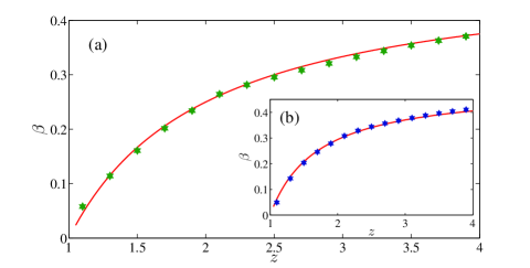
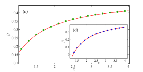
Figure 1: (Color online) Comparison between theoretical predictions (solid curves) and numerical results (symbols) for the subdiffusion exponent $\beta$ of the mean squared displacement $\langle(\delta h)^{2}(t)\rangle$ of the probe particle. The GEM (2) with $d=1$ is specified by the interaction kernel $\Lambda(r)\sim r^{-a_{1}}$ and correlated noise with $\Lambda^{\prime}(r)\sim r^{-a_{2}}$, where $\alpha_{1}$ and $\alpha_{2}$ for the different cases (a) to (d) depicted in panels (a) to (d) are chosen as (a) $\alpha_{1}=1$, $\alpha_{2}=1$; (b) $\alpha_{1}=0.7$, $\alpha_{2}=0.7$; (c) $\alpha_{1}=1$, $\alpha_{2}=0.7$; and (d) $\alpha_{1}=0.7$, $\alpha_{2}=1$.

In Fig. 1 we show numerical results for the subdiffusion exponent $\beta$ as function of the fractional order $z$ for the cases (a) to (d) introduced in Section II. The exponent is measured from the power-law dependence of the mean squared displacement with time, see the first equality in Eq. (24). The results of the numerical simulations are shown by the symbols, and the solid curves demonstrate the analytical result (20). We observe excellent agreement with the theoretical result for all our cases in the interesting range for $z$ between 1 and 4.

IV.2 Scaling properties of $q$th order moments

We now turn to the scaling properties of the $q$th order moments $\langle|\delta h(t)|^{q}\rangle$. According to the scale-invariance property,

$$h(s^{1/\nu}\mathbf{x},st)\equiv s^{\xi/\nu}h(\mathbf{x},t),\,\,\,s>0,$$ (25)

and the condition $\langle|\delta h(st)|^{q}\rangle=s^{q\xi/\nu}\langle|\delta h(t)|^{q}\rangle$, we find

$$\langle|\delta h(t)|^{q}\rangle\sim t^{\tau(q,\beta)},$$ (26)

where $\beta=\xi/\nu$ and $\tau(q,\beta)=q\beta$. When the exponent $\tau(q,\beta)$ is a linear function of $q$, the process is referred to as a mono-scale process, and the stochastic profile $h(\mathbf{x},t)$ is non-intermittent taqqu .

We studied the scaling behavior of the $q$-th moment numerically. In Fig. (2) $\tau(q,\beta)/q$ is plotted vs $q$ for the four paradigmatic examples, the cases (a)-(d). The figure shows that the $q^{-1}\tau(q,\beta)$ is equal to $\beta$ and independent of $q$, which demonstrates that the height fluctuations in the GEM are not intermittent.

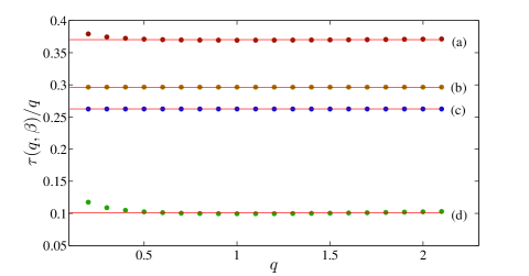
Figure 2: (Color online) The dots show the values of $q^{-1}\tau(q,\beta)$ obtained in numerical simulations of the GEM with interaction kernel $\Lambda(r)\sim r^{-\alpha_{1}}$ and correlated noise with $\Lambda^{\prime}(r)\sim r^{-\alpha_{2}}$. The parameters $\alpha_{1}$, $\alpha_{2}$ and $z$ correspond to the four cases (a)-(d) and are equal to: (a) $\alpha_{1}=1$, $\alpha_{2}=1$, $z=4.0$ (b) $\alpha_{1}=0.7$, $\alpha_{2}=0.7$, $z=2.0$ (c) $\alpha_{1}=1$, $\alpha_{2}=0.7$, $z=1.3$ (d)$\alpha_{1}=0.7$, $\alpha_{2}=1$, $z=1.5$. Solid lines show the corresponding values of the exponent $\beta$. This plot demonstrates the mono-scaling (non-intermittent) behavior of fluctuations.

IV.3 Ergodic properties

In the two previous Subsections we obtained the scaling exponents $\beta$ and $\tau(q,\beta)$ for the GEM with non-thermal initial condition. For this purpose we used the ensemble average of the second and $q$th order moments. For example, to determine the subdiffusion exponent $\beta$ one needs to obtain the ensemble average of the observable $(\delta h)^{2}$. In many experiments, however, one measures time averages of physical observables (see, for instance, Refs. He2008 ; burov2011 ). For an ergodic process, the long time average of an observable produces the same result as the corresponding ensemble average, while for a non-ergodic process the correct interpretation of the time average requires a separate theory. We here consider a single trajectory of length $T$ (measurement time) and define the time average as

$$\overline{\delta^{2}h(\Delta)}=\frac{1}{T-\Delta}\int_{0}^{T-\Delta}dt\left[h(x,t+\Delta)-h(x,t)\right]^{2},$$ (27)

where $\Delta$ denotes the lag time. It was shown in Ref. taloni2012 that the additional ensemble average $\langle\overline{\delta^{2}h}\rangle$ of the quantity (27) for systems with non-thermal initial condition tends to the value of the ensemble averaged MSD $\langle(\delta h)^{2}(t)\rangle_{\mathrm{st}}$ in the stationary state, if $\Delta/T\rightarrow 0$. This means that the process is ergodic, and sufficiently long time averages reproduce the exact behavior predicted by the ensemble quantities.

A useful quantity to measure the fluctuations between different realizations of a dynamic process is the probability density function of the amplitude scatter $\phi(\varepsilon)$ in terms of the dimensionless variable $\varepsilon=\overline{\delta^{2}h}/\langle\overline{\delta^{2}h}\rangle$ He2008 ; burov2011 ; jae . Thus, $\phi(\varepsilon)$ measures how reproducible individual realizations $\overline{\delta^{2}h}$ are with respect to the ensemble mean of the time averages, $\langle\overline{\delta^{2}h}\rangle$. For an ergodic system, $\phi(\epsilon)$ has bell shape around the ergodic value $\epsilon=1$, and for long measurement times $T$ it converges to a $\delta$-peak, $\lim_{T\to\infty}\phi(\epsilon)=\delta(\epsilon-1)$ He2008 ; jae .

Another measure of ergodic violation is the ergodicity breaking parameter He2008

$$\mathrm{EB}=\lim_{T\rightarrow\infty}\frac{\left<\left(\overline{\delta^{2}h}\right)^{2}\right>-\left<\overline{\delta^{2}h}\right>^{2}}{\left<\overline{\delta^{2}h}\right>^{2}}.$$ (28)

The sufficient condition for ergodicity is $\mathrm{EB}=0$.

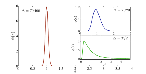
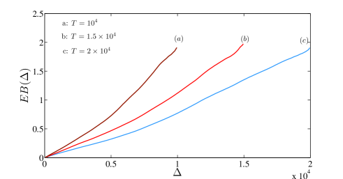
Figure 3: (Color online) Top panel: Probability density function of the scaled random variable $\epsilon=\overline{\delta^{2}h}/\langle\overline{\delta^{2}h}\rangle$ for different values of the lag time $\Delta$. The measurement time $T=2\times 10^{4}$. Bottom panel: Ergodicity breaking parameter $\mathrm{EB}$ as a function of the lag time $\Delta$ for three different values of $T$.

Here we restrict ourselves to the special case (b). To study the ergodic properties of the GEM, we calculate the amplitude scatter PDF $\phi(\epsilon)$ and the ergodicity breaking parameter $\mathrm{EB}$. In the top panel of Fig. 3 we show that the shape of $\phi(\epsilon)$ becomes sharper with decreasing $\Delta$ when the measurement time $T$ is fixed. In the limit $\Delta\ll T$, the PDF has a peak close to the ergodic value $\overline{\delta^{2}h}/\langle\overline{\delta^{2}h}\rangle=1$, which indicates the ergodicity of the process. In the bottom panel of Fig. 3 we depict the ergodicity breaking parameter $\mathrm{EB}$ as a function of the lag time $\Delta$ for different values of the measurement time $T$. We see that indeed the ergodicity breaking parameter converges to the ergodic value $\mathrm{EB}\rightarrow 0$ for $\Delta/T\rightarrow 0$.

IV.4 The GEM with localized perturbation

In the preceding Section IV we studied the properties of the unbiased GEM. We now report results of numerical simulations of the driven GEM with a constant localized perturbation, $\mathbf{F}\{h(\mathbf{x}^{\prime},t),t\}=F_{0}\Theta(t)$, compare Eq. (5). We consider the motion of a tagged probe located at $x^{\star}$. The results for an untagged probe will be presented elsewhere. Obviously, the stochastic term in Eq. (5) does not make a contribution to the average drift $\langle h(\mathbf{x}^{\star},t)\rangle_{F_{0}}$, since $\langle\eta(x,t)\rangle=0$. Thus, basically, the average drift is determined by the nature of the hydrodynamic friction kernel $\Lambda(r)$. Following Refs. taloni2011 ; taloni2013 we determine the average drift,

$$\langle h(\mathbf{x}^{\star},t)\rangle_{F_{0}}\propto F_{0}t^{2\beta^{\prime}},$$ (29)

where the dynamic scaling exponent is $\beta^{\prime}=(z-d)/2z$ for the local and $\beta^{\prime}=(z-d)/2(z+\alpha-d)$ for the non-local hydrodynamic interaction, where the former expression holds for the cases (a) and (c), while the latter formula is valid for the cases (b) and (d). Note that $\beta^{\prime}=\beta$ for the GEM obeying the fluctuation-dissipation relation of the second kind, corresponding to local hydrodynamic interaction and uncorrelated noise [case (a)] and that with non-local interaction and correlated noise [case (b)]. Thus, the Einstein relation

$$\langle h(\mathbf{x}^{\star},t)\rangle_{F_{0}}=\frac{\langle(\delta h)^{2}(t)\rangle_{\mathrm{st}}}{2k_{B}T}F_{0}$$ (30)

holds for the tagged probe in the two cases (a) and (b), where $\langle(\delta h)^{2}(t)\rangle_{\mathrm{st}}$ is defined by Eq. (24).

We simulated the GEM with constant local force on a one-dimensional lattice, see Eq. (15). Then we calculate the average drift and extract the dynamic exponent $\beta^{\prime}$ according to Eq. (29). The results are shown in Fig. 4. The main panel depicts $\beta^{\prime}$ as a function of $z$ for local [case (a)] and non-local [case (b] interactions. The results of the simulations shown by the symbols perfectly agree with the analytical findings (solid curves), i.e., $\beta^{\prime}=(z-1)/2z$ for the local and $\beta^{\prime}=(z-1)/2(z+\alpha-1)$ for the non-local case, respectively. In addition, in the insets we show $\langle h(\mathbf{x}^{\star},t)\rangle_{F_{0}}$ as a function of the applied force $F_{0}$ for several values of $z$.

Figure 4: (Color online) Dynamic scaling exponent $\beta^{\prime}$ for the GEM with local [cases (a) and (c)] and nonlocal [cases (b) and (d), with $\alpha=0.7$] hydrodynamic interaction. Main panel: numerical results are shown by the symbols, whereas the solid (red) lines correspond to the theoretical relations $\beta^{\prime}=(z-1)/2z$ and $(z-1)/2(z+\alpha-1)$ for the two cases (a) and (b), respectively. Insets: The relation between $\langle h(x^{\star},t)\rangle_{F_{0}}$ and $F_{0}$ for the tagged tracer in the GEM [cases (a) and (b)] for different fractional order $z$. Solid red lines correspond to the analytical expression $t^{-2\beta^{\prime}}\langle h(x^{\star},t)\rangle_{F_{0}}=\frac{K}{k_{B}T}F_{0}$ [see Eqs. (29) and (30)].

V Conclusions and Discussions

In this paper, we studied the interface dynamics of the generalized elastic model with two types of interactions, local and long-range non-local ones, in the presence of uncorrelated as well as long-range correlated noise. We generalized some of the previous results from Taloni et al. taloni2010 ; taloni2012 ; taloni2011 on the scaling properties of the GEM, and we developed a discrete numerical scheme to simulate the one-dimensional GEM on the lattice by using a discretized version of the Riesz-Feller fractional operator. We performed numerical simulations and measured the dynamics scaling exponents $\beta$ for the second moment and $\tau(q,\beta)$ for the $q$th order moments of the random field $h$ for four paradigmatic cases of the GEM. We also analyzed the ergodic properties of the GEM and demonstrated the ergodicity of the process by measuring the amplitude scatter of individual trajectories and the ergodicity breaking parameter. Finally, we simulated the driven GEM with localized perturbation and measured the scaling exponent $\beta^{\prime}$ from the scaling properties of the mean drift of a tagged probe. All numerical results are in perfect agreement with the analytics, thus supporting the numerical scheme developed herein.

It will be interesting to apply this numerical algorithm to other relevant aspects of interface dynamics, such as the presence of quenched disorder, and GEM with nonlinear terms. Another direction is to develop numerical tools to study the GEM in higher dimensions.

Appendix A The matrix transform method

The discrete space fractional operator can be efficiently generated by the matrix transform algorithm proposed in Refs. yang ; ilic2005 . This method is based on the following definition ilic2005 : Consider the Laplacian $(-\Delta)$ on a bounded region $\mathfrak{D}$, with a complete set of orthonormal eigenfunctions $\phi_{n}$ and eigenvalues $\lambda^{2}_{n}$, i.e., $(-\Delta)\phi_{n}=\lambda^{2}_{n}\phi_{n}$. An orthogonal and complete set of functions $\{\phi_{n}\}$ may be used to expand an arbitrary function $f(\textbf{x})$ in the following form

$$f=\sum_{n=1}^{\infty}c_{n}\phi_{n},\quad\text{with }c_{m}=\int_{\mathfrak{D}}\phi_{n}(\textbf{x})f(\textbf{x})d\textbf{x}.$$ (31)

Then, for any $f$ one can define $(-\Delta)^{z/2}$ as

$$(-\Delta)^{z/2}f=\sum_{n=1}^{\infty}c_{n}\lambda^{z}_{n}\phi_{n}.$$ (32)

It is worthwhile mentioning that the complete set of functions $\{\phi_{n}\}$ is also the eigensolution of the fractional operator, $(-\Delta)^{z/2}\phi_{n}=\lambda^{z}_{n}\phi_{n}$. This definition provides a new method and corresponding numerical scheme to approximate a space-fractional operator.

Appendix B The modified Fourier filtering method

The celebrated fractional Gaussian noise can be efficiently generated by the algorithm proposed in Ref. makse1996 . Consider the noise $\eta(x,t)$ with the correlation function

$$\langle\eta(x,t)\eta(x^{\prime},t^{\prime})\rangle\propto\Lambda^{\prime}(r)\delta{(t-t^{\prime})},$$ (33)

where $r=|x-x^{\prime}|$ and $\Lambda^{\prime}(r)\sim r^{-\alpha}$ in the limit $r\rightarrow\infty$. For the fixed time instant $t_{n}$, the noise is generated on a uniform, one-dimensional grid with $L$ points. Following the discrete Fourier transformation, the Fourier component of the correlated noise $\eta(x_{i},t_{n})$ is defined by

$$\eta(q,t_{n})=\sum_{x_{i}=-L/2}^{L/2}\eta(x_{i},t_{n})e^{-iqx_{n}},$$ (34)

where $q$ assumes the values $q=2\pi m/L$ with $m=\{-L/2,\dots,L/2\}$. The idea of the Fourier filtering method is to simulate a process $\eta(q,t_{n})$ with the spectral density

$$\Lambda^{\prime}(q)=\langle\eta(q,t_{n})\eta(-q,t_{n})\rangle\sim q^{\alpha-1},$$ (35)

for $q\rightarrow 0$, and transform the resulting series to real space. The correlated noise is then constructed by filtering the Fourier components of a sequence of normally distributed random numbers $\{w_{i}\}_{i=1,\dots,L}$ with the correlation function $\langle w_{i}w_{j}\rangle\sim\delta_{i,j}$ and the Fourier transform $w_{q}$. Then one generates the Fourier transform coefficients of the correlated noise by

$$\eta(q,t_{n})=\left[\Lambda^{\prime}(q)\right]^{1/2}w_{q}.$$ (36)

References

- (1) P. Meakin, Fractals, Scaling and Growth far from Equilibrium (Cambridge University Press, Cambridge, UK, 1998).
- (2) A. L. Barabśi and H. E. Stanley, Fractal Concepts in Surface Growth (Cambridge University Press, Cambridge, UK, 1995)
- (3) R. Granek, J. de Physique II 7, 1761 (1997); R. Granek and J. Klafter, Europhys. Lett. 56, 15 (2007).
- (4) L. Lizana, T. Ambjörnsson, A. Taloni, E. Barkai, and M. A. Lomholt, Phys. Rev. E 81, 051118 (2010); M. A. Lomholt, L. Lizana, and T. Ambjörnsson, J. Chem. Phys. 134, 045101 (2011).
- (5) A. G. Zilman and R. Granek, Chem. Phys. 284, 195 (2002).
- (6) E. Helfer, S. Harlepp, L. Bourdieu, J. Robert, F. MacKintosh, and D. Chatenay, Phys. Rev. Lett. 85, 457 (2000).
- (7) M. Doi and S. F. Edwards, The Theory of Polymer Dynamics (Clarendon Press, Oxford, UK, 1986).
- (8) F. Amblard, A. C. Maggs, B. Yurke, A. N. Pargellis, and S. Leibler, Phys. Rev. Lett. 77, 4470 (1996).
- (9) R. Everaers, F. Jülicher, A. Ajdari, and A. Maggs, Phys. Rev. Lett. 82, 3717 (1999).
- (10) A. Caspi, M. Elbaum, R. Granek, A. Lachish, and D. Zbaida, Phys. Rev. Lett. 80, 1106 (1998).
- (11) S. Buldyrev, A.-L. Barabási, F. Caserta, S. Havlin, H. Stanley, and T. Vicsek, Phys. Rev. A 45, 8313 (1992).
- (12) J. Nissen, K. Jacobs, and J. O. Rädler, Phys. Rev. Lett. 86, 1904 (2001).
- (13) S. Bustingorry, L. F. Cugliandolo, and D. Dominguez, Phys. Rev. Lett. 96, 27001 (2006); U. Dobramysl, H. Assi, M. Pleimling, and U. C. Täuber, arXiv preprint arXiv:1211.6929 (2012).
- (14) A. Brú, J. M. Pastor, I. Fernaud, I. Brú, S. Melle, and C. Berenguer, Phys. Rev. Lett. 81, 4008 (1998).
- (15) I. Podlubny, Fractional Differential Equations (Academic Press, London, UK, 1999).
- (16) N. G. van Kampen, Stochastic processes in chemistry and physics (North Holland, Amsterdam, NL, 1981).
- (17) A. Taloni, A. Chechkin, and J. Klafter, Phys. Rev. Lett. 104, 160602 (2010); Rev. E 82, 061104 (2010).
- (18) A. Taloni, A. Chechkin, and J. Klafter, Europhys. Lett. 97, 30001 (2012).
- (19) A. Taloni, A. Chechkin, and J. Klafter, Phys. Rev. E 84, 021101 (2011).
- (20) A. Taloni, A. Chechkin, and J. Klafter, Mathematic. Modeling Nat. Phenomena 8, 127 (2013).
- (21) In the present work the exponent corresponds to from Taloni et al. taloni2010 ; taloni2012 ; taloni2011 ; taloni2013 .
- (22) L. C. E. Struik, Physical aging in amorphous polymers and other materials, vol. 106 (Elsevier Amsterdam, The Netherlands, 1978).
- (23) J.-P. Bouchaud and A. Georges, Phys. Rep. 195, 127 (1990).
- (24) R. Metzler and J. Klafter, Phys. Rep. 339, 1 (2000); J. Phys. A 37, R161 (2004).
- (25) J. P. Bouchaud, J. de Physique I 2, 1705 (1992).
- (26) L. Cugliandolo and J. Kurchan, Philos. Mag. B 71, 501 (1995).
- (27) C. Monthus and J.-P. Bouchaud, J. Phys. A 29, 3847 (1996).
- (28) B. Rinn, P. Maass, and J.-P. Bouchaud, Phys. Rev. Lett. 84, 5403 (2000).
- (29) E. Barkai, Phys. Rev. Lett. 90, 104101 (2003).
- (30) G. Bel and E. Barkai, Phys. Rev. Lett. 94, 240602 (2005).
- (31) A. Rebenshtok and E. Barkai, Phys. Rev. Lett. 99, 210601 (2007); J. Stat. Phys. 133, 565 (2008).
- (32) J. H. P. Schulz, E. Barkai, and R. Metzler, Phys. Rev. Lett. 110, 020602 (2013).
- (33) Y. He, S. Burov, R. Metzler, and E. Barkai, Phys. Rev. Lett. 101, 058101 (2008); A. Lubelski, I. M. Sokolov, and J. Klafter, Phys. Rev. Lett. 100, 250602 (2008).
- (34) S. Burov, J.-H. Jeon, R. Metzler, and E. Barkai, Phys. Chem. Chem. Phys. 13, 1800 (2011); J.-H. Jeon, E. Barkai, and R. Metzler, J. Chem. Phys. 139, 121916 (2013); E. Barkai, Y. Garini, and R. Metzler, Phys. Today 65(8), 29 (2012).
- (35) S. M. A. Tabei, S. Burov, H. Y. Kim, A. Kuznetsov, T. Huynh, J. Jureller, L. H. Philipson, A. R. Dinner, and N. F. Scherer, Proc. Natl. Acad. Sci. USA 110, 4911 (2013); A. V. Weigel, B. Simon, M. M. Tamkun, and D. Krapf, ibid. 108, 6438 (2011); J.-H. Jeon, V. Tejedor, S. Burov, E. Barkai, C. Selhuber-Unkel, K. Berg-Sørensen, L. Oddershede, and R. Metzler, Phys. Rev. Lett. 106, 048103 (2011); I. Y. Wong, M. L. Gardel, D. R. Reichman, E. R. Weeks, M. T. Valentine, A. R. Bausch, and D. A. Weitz, ibid. 92, 178101 (2004); Q. Xu, L. Feng, R. Sha, N. C. Seeman, and P. M. Chaikin, ibid. 106, 228102 (2011).
- (36) A. G. Cherstvy, A. V. Chechkin, and R. Metzler, New J. Phys. 15, 083039 (2013); A. G. Cherstvy and R. Metzler, E-print arXiv:1307.6407.
- (37) M. A. Lomholt, L. Lizana, R. Metzler, and T. Ambjörnsson, Phys. Rev. Lett. 110, 208301 (2013).
- (38) W. Deng and E. Barkai, Phys. Rev. E 79, 011112 (2009); J.-H. Jeon and R. Metzler, ibid. 81, 021103 (2010).
- (39) J. Kursawe, J. H. P. Schulz, and R. Metzler, E-print arXiv:1307.6131; J-.H. Jeon, N. Leijnse, L. Oddershede, and R. Metzler, New J. Phys. 15, 045011 (2013); J.-H. Jeon and R. Metzler, Phys. Rev. E 85, 021147 (2012).
- (40) S. G. Samko, A. A. Kilbas, and O. O. I. Marichev, Fractional integrals and derivatives (Gordon and Breach, New York, NY, 1993).
- (41) Y.-K. Yu, N.-N. Pang, and T. Halpin-Healy, Phys. Rev. E 50, 5111 (1994).
- (42) N.-N. Pang, Phys. Rev. E 56, 6676 (1997).
- (43) N.-N. Pang and W.-J. Tzeng, Phys. Rev. E 82, 031605 (2010).
- (44) J. Krug, H. Kallabis, S. Majumdar, S. Cornell, A. Bray, and C. Sire, Phys. Rev. E 56, 2702 (1997).
- (45) S. N. Majumdar and A. J. Bray, Phys. Rev. Lett. 86, 3700 (2001).
- (46) A. A. Kilbas, H. M. Srivastava, and J. J. Trujillo, Theory and Applications of Fractional Differential Equations, vol. 204 (Elsevier, 2006).
- (47) Q. Yang, Novel analytical and numerical methods for solving fractional dynamical systems (Ph.D. Thesis, Queesland University of Technology, Australia, http://eprints.qut.edu.au/35750, 2010).
- (48) A. I. Saichev and G. M. Zaslavsky, Chaos 7, 753 (1997).
- (49) M. Ilic, F. Liu, I. Turner, and V. Anh, Fractl. Calc. and Appl. Anal. 8, 323 (2005); ibid. 9, 333 (2006).
- (50) A. Zoia, A. Rosso, and M. Kardar, Phys. Rev. E 76, 021116 (2007).
- (51) H.-O. Peitgen, D. Saupe, M. F. Barnsley, Y. Fisher, and M. McGuire, The science of fractal images (Springer, New York, NY, 1988).
- (52) M. Ausloos and D. Berman, Proc. Roy. Soc. (London) A 400, 331 (1985).
- (53) H. Hamzehpour and M. Sahimi, Phys. Rev. E 73, 056121 (2006).
- (54) H. A. Makse, S. Havlin, M. Schwartz, and H. E. Stanley, Phys. Rev. E 53, 5445 (1996).
- (55) M. S. Taqqu and G. Samorodnisky, Stable non-Gaussian random processes (Chapman and Hall, New-York, NY, 1994).
- (56) J.-H. Jeon and R. Metzler, J. Phys. A 43, 252001 (2010).