Adaptive Metropolis Algorithm Using Variational Bayesian Adaptive Kalman Filter

Abstract

Markov chain Monte Carlo (MCMC) methods are powerful computational tools for analysis of complex statistical problems. However, their computational efficiency is highly dependent on the chosen proposal distribution, which is generally difficult to find. One way to solve this problem is to use adaptive MCMC algorithms which automatically tune the statistics of a proposal distribution during the MCMC run. A new adaptive MCMC algorithm, called the variational Bayesian adaptive Metropolis (VBAM) algorithm, is developed. The VBAM algorithm updates the proposal covariance matrix using the variational Bayesian adaptive Kalman filter (VB-AKF). A strong law of large numbers for the VBAM algorithm is proven. The empirical convergence results for three simulated examples and for two real data examples are also provided.

1 Introduction

Markov chain Monte Carlo (MCMC) methods [10] are an important class of numerical tools for approximating multidimensional integrals over complicated probability distributions in Bayesian computations and in various other fields. The computational efficiency of MCMC sampling depends on the choice of the proposal distribution. A challenge of MCMC methods is that in complicated high-dimensional models it is very hard to find a good proposal distribution.

The Gaussian distribution is often used as a proposal distribution due to its theoretical and computational properties. However, the Gaussian proposal distribution needs a well tuned covariance matrix for optimal acceptance rate and good mixing of the Markov chain. If the covariance matrix is too small, too large or has improper correlation structure, the Markov chains will be highly positively correlated and hence the estimators will have a large variance. Because manual tuning is laborious, several adaptive MCMC algorithms have been suggested [20, 21, 19, 37, 2, 30, 31, 4, 14] to update the covariance matrix during the MCMC run.

In this article, we propose a new adaptive Metropolis algorithm, where we update the covariance matrix of the Gaussian proposal distribution of the Metropolis algorithm using the variational Bayesian adaptive Kalman filter (VB-AKF) proposed by Särkkä and Nummenmaa [35] and Särkkä and Hartikainen [34]. The idea of the classical Metropolis algorithm [20] is essentially to empirically estimate the covariance of the samples and use this estimate to construct the proposal distribution. However, as we point out here, such a covariance estimation problem can also be formulated as an instance of recursive Bayesian estimation, where the term used for this kind of recursive estimation is Bayesian filtering [33]. This reinterpretation allows one to construct alternative and potentially more effective adaptation mechanisms by utilizing the various Bayesian filtering algorithms developed over the years for doing the covariance estimation. The aim of this article is to propose a practical algorithm which is constructed from this underlying idea, prove its convergence, and test its performance empirically.

The structure of this article is the following: in Section 2 we review the existing adaptive MCMC methods. Section 3 is dedicated to our new adaptive Metropolis algorithm. Theoretical validity of the proposed algorithm is shown in Section 4 by proving a strong law of large numbers. In Section 5, we study the empirical convergence of the method in three simulated examples and then apply the method to two real data examples.

2 Adaptive Markov Chain Monte Carlo Methods

Markov chain Monte Carlo (MCMC) methods are widely used algorithms for drawing samples from complicated multidimensional probability distributions. For example, in Bayesian analysis [13], we are often interested in computing the posterior expectation of a function $\mathbf{g}(\boldsymbol{\theta})$ given the measurements $\mathbf{z}_{1},\ldots,\mathbf{z}_{M}$:

$$\mathrm{E}[\mathbf{g}(\theta)\mid\mathbf{z}_{1},\ldots,\mathbf{z}_{M}]=\int_{\mathbb{R}^{d}}\mathbf{g}(\theta)\,p(\theta\mid\mathbf{z}_{1},\ldots,\mathbf{z}_{M})\,\mathrm{d}\theta.$$ (1)

We can use MCMC methods to approximate the expectation by drawing samples from the posterior distribution

$$\boldsymbol{\theta}_{1},\boldsymbol{\theta}_{2},\ldots,\boldsymbol{\theta}_{n}\sim p(\boldsymbol{\theta}\mid\mathbf{z}_{1},\ldots,\mathbf{z}_{M}),$$ (2)

and then by employing the approximation

$$\mathrm{E}[\mathbf{g}(\boldsymbol{\theta})\mid\mathbf{z}_{1},\ldots,\mathbf{z}_{M}]\approx\frac{1}{n}\sum_{i=1}^{n}\mathbf{g}(\boldsymbol{\theta}_{i}).$$ (3)

A common construction for MCMC uses a random walk that explores the state space through local moves. The most well-known traditional MCMC method is the Metropolis algorithm. In the Metropolis algorithm we draw a candidate point $\boldsymbol{\theta}_{*}$ from a symmetric proposal distribution $q(\boldsymbol{\theta}_{*}\mid\boldsymbol{\theta})$ and use an accept/reject rule to accept or reject the sampled point [15, 13, 10].

The efficiency of an MCMC algorithm can be improved by carefully tuning the proposal distribution. Adaptive MCMC methods are a family of algorithms, which take care of the tuning automatically. This proposal is often chosen to be a Gaussian distribution, in which case it is the covariance matrix that needs to be tuned. Under certain settings Gelman et al. [14] show that the optimal covariance matrix for an MCMC algorithm with Gaussian proposal is $\lambda\,\boldsymbol{\Sigma}$, with $\lambda=2.38^{2}/d$, where $d$ is the dimension and $\boldsymbol{\Sigma}$ is the $d\times d$ covariance matrix of the target distribution.

In the adaptive Metropolis (AM) algorithm by Haario et al. [21], the covariance matrix $\boldsymbol{\Sigma}_{k-1}$ for the step $k$ is estimated as follows:

$$\boldsymbol{\Sigma}_{k-1}=\text{cov}(\boldsymbol{\theta}_{0},\boldsymbol{\theta}_{1},\ldots,\boldsymbol{\theta}_{k-1})+\epsilon\mathbf{I},$$ (4)

where $\mathbf{I}$ is the $d\times d$ identity matrix and $\epsilon$ is a small positive value whose role is to make sure that $\boldsymbol{\Sigma}_{k-1}$ is not singular [20, 21]. The AM algorithm of Haario et al. [21] can be summarized as follows:

• Initialize $\boldsymbol{\theta}_{0}$, $\boldsymbol{\Sigma}_{0}$.

• For $k=1,2,3,\ldots$

  • Sample a candidate point $\boldsymbol{\theta}_{*}$ from a Gaussian distribution

    $$\boldsymbol{\theta}_{*}\sim\mathbb{N}(\boldsymbol{\theta}_{k-1},\lambda\,\boldsymbol{\Sigma}_{k-1}).$$ (5)

  • Compute the acceptance probability

    $$\alpha_{k}=\text{min}\left\{1,\,\frac{p(\boldsymbol{\theta}_{*}\mid\mathbf{z}_{1},\ldots,\mathbf{z}_{M})}{p(\boldsymbol{\theta}_{k-1}\mid\mathbf{z}_{1},\ldots,\mathbf{z}_{M})}\right\}.$$ (6)

  • Sample a random variable $u$ from the uniform distribution $\mathbb{U}(0,1)$.

  • If $u<\alpha_{k}$, set $\boldsymbol{\theta}_{k}=\boldsymbol{\theta}_{*}$. Otherwise set $\boldsymbol{\theta}_{k}=\boldsymbol{\theta}_{k-1}$.

  • Compute the covariance matrix $\boldsymbol{\Sigma}_{k}$ using Equation (4).

Different adaptive algorithms have been proposed as improved versions of the AM algorithm above. Good surveys of such algorithms are found in Andrieu and Thoms [2], Liang et al. [26], where the authors present ways to implement the algorithms and then show why the algorithms preserve the correct stationary distributions. For instance, apart from updating the covariance alone, one can adapt $\lambda$ using the following Robbins–Monro algorithm, which alleviates the problem of $\boldsymbol{\Sigma}_{k}$ being systematically too large or too small [2, 3, 36]:

$$\log(\lambda_{k})=\log(\lambda_{k-1})+\gamma_{k}\,(\alpha_{k}-\overline{\alpha}).$$ (7)

In Equation (7), $\overline{\alpha}$ is the target acceptance rate which is commonly set to 0.234 and $\gamma_{k}$ is a gain factor sequence satisfying the following conditions:

$$\sum_{k=1}^{\infty}\gamma_{k}=\infty\quad\text{and}\quad\sum_{k=1}^{\infty}\gamma_{k}^{1+\delta}<\infty\quad\text{ for some }\delta\in(0,1].$$

In a recent paper, Vihola [37] introduced the robust adaptive Metropolis (RAM) algorithm with an online rule for adapting the covariance matrix and a mechanism for maintaining the mean acceptance rate at a pre-determined level. Holden et al. [23] describe an adaptive independent Metropolis–Hastings algorithm, where the proposal is adapted with past samples. The limitation of this adaptation is that the information gained from doing the local steps cannot be used, so the algorithm iterations do not improve the proposal [23, 26]. Gilks et al. [17] proposed regeneration-based adaptive algorithms, where after each regeneration point the proposal distribution is modified based on all the past samples and the future outputs become independent of the past. In the population-based adaptive algorithms the proposal distributions are designed such that computational techniques are incorporated into simulations and the covariance matrix is adapted using a population of independent and identically distributed samples from the adaptive direction sampler [16] or the evolutionary Monte Carlo [28].

Another type of adaptive MCMC is proposed by Vrugt et al. [39] and Vrugt and Braak [38], where they integrate the MCMC algorithm and differential evolution. This type of algorithm generates multiple different chains simultaneously for global exploration, and automatically tunes the scale and orientation of the proposal distribution in randomized subspaces during the search. One way of adapting the MCMC proposal distribution is by using multiple copies of the target density and Gibbs sampling [11, 18]. The idea is that a product of the proposal density and copies of the target density is used to define a joint density which is sampled by Metropolis–Hastings-within-Gibbs algorithm.

When constructing an adaptive algorithm one should be sure that the conditions for ergodicity are satisfied to ensure that the algorithm converges to the target distribution [1, 30, 32, 3, 6]. One way to ensure the ergodicity property of adaptive MCMC is in terms of the two general conditions [5, 6]: diminishing adaptation and containment condition. However, these conditions are not necessary and there exist valid adaptation mechanisms that do not have these properties. In our proposed algorithm, to ensure ergodicity, we impose slightly stronger conditions that imply the diminishing and containment conditions. The imposed conditions also imply a strong law of large numbers rather than just a weak law of large numbers.

3 Adaptive Metropolis Algorithm with Variational Bayesian Adaptive Kalman Filter Based Covariance Update

In this section, we first briefly review the noise adaptive Kalman filter [34] which is used to adapt the covariance matrix of the proposal distribution, and then present the proposed variational Bayesian adaptive Metropolis (VBAM) algorithm.

3.1 Kalman Filter

Kalman filter [25] is the classical algorithm for estimation of the dynamic state from noisy measurements in linear Gaussian state space models. In probabilistic terms the model can be expressed as [24, 33]

$$\mathbf{x}_{k} \sim\mathbb{N}(\mathbf{A}_{k-1}\,\mathbf{x}_{k-1},\mathbf{Q}_{k-1}),$$

$$\mathbf{y}_{k} \sim\mathbb{N}(\mathbf{H}_{k}\,\mathbf{x}_{k},\boldsymbol{\Sigma}_{k}),$$

where $\mathbb{N}(\cdot)$ denotes the multivariate Gaussian distribution, $\mathbf{x}_{k}\in\mathbb{R}^{n}$ is the dynamic state, $\mathbf{A}_{k-1}$ is the dynamic model matrix, $\mathbf{Q}_{k-1}$ is the process noise covariance, $\mathbf{y}_{k}\in\mathbb{R}^{d}$ is the measurement, $\mathbf{H}_{k}$ is the measurement matrix, and $\boldsymbol{\Sigma}_{k}$ is the measurement noise covariance matrix. Here, $\mathbf{x}_{k}$ is an unknown variable and $\mathbf{y}_{k}$ is an observed variable, whereas the matrices $\mathbf{A}_{k-1}$, $\mathbf{Q}_{k-1}$, $\mathbf{H}_{k}$, and $\boldsymbol{\Sigma}_{k}$ are assumed known. We further assume that $\mathbf{x}_{0}\sim\mathbb{N}(\mathbf{m}_{0},\mathbf{P}_{0})$, where $\mathbf{m}_{0}$ and $\mathbf{P}_{0}$ are the known prior mean and covariance. The estimation of states is recursively performed using two Kalman filter steps:

1. Prediction step:

   $$\begin{split}\mathbf{m}_{k}^{-}&=\mathbf{A}_{k-1}\,\mathbf{m}_{k-1},\\ \mathbf{P}_{k}^{-}&=\mathbf{A}_{k-1}\,\mathbf{P}_{k-1}\,\mathbf{A}^{T}_{k-1}+\mathbf{Q}_{k-1}.\end{split}$$ (8)

2. Update step:

   $$\begin{split}\mathbf{S}_{k}&=\mathbf{H}_{k}\,\mathbf{P}_{k}^{-}\,\mathbf{H}_{k}^{T}+\boldsymbol{\Sigma}_{k},\\ \mathbf{K}_{k}&=\mathbf{P}_{k}^{-}\,\mathbf{H}_{k}^{T}\,\mathbf{S}_{k}^{-1},\\ \mathbf{m}_{k}&=\mathbf{m}_{k}^{-}+\mathbf{K}_{k}\,\left(\mathbf{y}_{k}-\,\mathbf{H}_{k}\,\mathbf{m}_{k}^{-}\right),\\ \mathbf{P}_{k}&=\mathbf{P}_{k}^{-}-\mathbf{K}_{k}\,\mathbf{S}_{k}\,\mathbf{K}_{k}^{T},\end{split}$$ (9)

where $\mathbf{m}_{k}^{-}$ is the a priori state mean, $\mathbf{m}_{k}$ is the a posteriori state mean, $\mathbf{P}_{k}^{-}$ is the a priori state covariance, and $\mathbf{P}_{k}$ is the a posteriori state covariance. In Bayesian sense the Kalman filter computes the statistics for the following conditional distribution of the state given the measurements:

$$p(\mathbf{x}_{k}\mid\mathbf{y}_{1:k})=\mathbb{N}(\mathbf{x}_{k}\mid\mathbf{m}_{k},\mathbf{P}_{k}).$$ (10)

If $\mathbf{A}_{k-1}=\mathbf{I}$ and the process noise is zero $\mathbf{Q}_{k-1}=\mathbf{0}$, the Kalman filter reduces to the so called recursive least squares (RLS) algorithm which solves a general multivariate linear estimation (regression) problem recursively. The matrices $\mathbf{A}_{k-1}$ and $\mathbf{Q}_{k-1}$ can be used for modeling the dynamics of the state when it is not assumed to be static (as in RLS).

3.2 Variational Noise Adaptation

In the Kalman filter discussed above, the model matrices in the state space model are assumed to be known. The variational Bayesian adaptive Kalman filter (VB-AKF, [35, 34]) is considered with the case where the noise covariance $\boldsymbol{\Sigma}_{k}$ is unknown. The model is assumed to be of the form:

$$\mathbf{x}_{k} \sim\mathbb{N}(\mathbf{A}_{k-1}\,\mathbf{x}_{k-1},\mathbf{Q}_{k-1}),$$ (11)

$$\mathbf{y}_{k} \sim\mathbb{N}(\mathbf{H}_{k}\mathbf{x}_{k},\boldsymbol{\Sigma_{k}}),$$ (12)

$$\boldsymbol{\Sigma}_{k} \sim p(\boldsymbol{\Sigma}_{k}\mid\boldsymbol{\Sigma}_{k-1}),$$ (13)

where Equation (13) defines the Markovian dynamic model prior for the unknown measurement noise covariances. If we were able to implement the optimal (non-Gaussian) Bayesian filter for this model, it would compute the distribution

$$p(\mathbf{x}_{k},\boldsymbol{\Sigma}_{k}\mid\mathbf{y}_{1:k}).$$ (14)

Recall that the Kalman filter can be considered as a generalization of the RLS algorithm. In the same way we can consider the Bayesian filter for the above model as a generalization of the RLS algorithm where the noise variance is estimated together with the linear regression solution. We can also interpret the AM covariance adaption rule in Equation (4) as a simple linear regression problem where we estimate the noise covariance together with the linear regression solution. However, in AM we throw out the linear regression solution and only retain the covariance.

Because the above model is a generalization of RLS with covariance estimation, it can be seen to provide a recursive solution for estimation of the covariance in Equation (4) as a special case. This is the idea of our method. However, there is no reason to only use the parameters which reduce the Bayesian filter to the RLS, but one can use the full state space model and the corresponding filter to construct an adaptive Metropolis algorithm.

Unfortunately, the exact Bayesian filter for the above model is computationally intractable. However, the joint filtering distribution of the state and covariance matrix can be approximated with the free-form variational Bayesian approximation as follows [35, 34]:

$$p(\mathbf{x}_{k},\boldsymbol{\Sigma}_{k}\mid\mathbf{y}_{1:k})\approx Q_{\mathbf{x}}(\mathbf{x}_{k})\,Q_{\boldsymbol{\Sigma}}(\boldsymbol{\Sigma}_{k}),$$ (15)

where $Q_{\mathbf{x}}(\mathbf{x}_{k})$ and $Q_{\boldsymbol{\Sigma}}(\boldsymbol{\Sigma}_{k})$ are unknown approximating densities formed by minimizing the Kullback–Leibler (KL) divergence between the true distribution and the approximation:

$$\begin{split}&\textrm{KL}\left[Q_{\mathbf{x}}(\mathbf{x}_{k})Q_{\boldsymbol{\Sigma}}(\boldsymbol{\Sigma}_{k})\,||\,p(\mathbf{x}_{k},\boldsymbol{\Sigma}_{k}\mid\mathbf{y}_{1:k})\right]\\ &\qquad=\int Q_{\mathbf{x}}(\mathbf{x}_{k})\,Q_{\boldsymbol{\Sigma}}(\boldsymbol{\Sigma}_{k})\,\log\left(\frac{Q_{\mathbf{x}}(\mathbf{x}_{k})\,Q_{\boldsymbol{\Sigma}}(\boldsymbol{\Sigma}_{k})}{p(\mathbf{x}_{k},\boldsymbol{\Sigma}_{k}\mid\mathbf{y}_{1:k})}\right)\,\mathrm{d}\mathbf{x}\,\mathrm{d}\boldsymbol{\Sigma}_{k}.\end{split}$$ (16)

The KL divergence above can be minimized with respect to $Q_{\mathbf{x}}(\mathbf{x}_{k})$ and $Q_{\boldsymbol{\Sigma}}(\boldsymbol{\Sigma}_{k})$ using the methods from calculus of variations, which results in the following approximations [35, 34]:

$$Q_{\mathbf{x}}(\mathbf{x}_{k}) \propto\exp\left(\int\log p(\mathbf{x}_{k},\boldsymbol{\Sigma}_{k}\mid\mathbf{y}_{1:k})\,Q_{\boldsymbol{\Sigma}}(\boldsymbol{\Sigma}_{k})\,\mathrm{d}\boldsymbol{\Sigma}_{k}\right),$$ (17)

$$Q_{\boldsymbol{\Sigma}}(\boldsymbol{\Sigma}_{k}) \propto\exp\left(\int\log p(\mathbf{x}_{k},\boldsymbol{\Sigma}_{k}\mid\mathbf{y}_{1:k})\,Q_{\mathbf{x}}(\mathbf{x}_{k})\,\mathrm{d}\mathbf{x}_{k}\right).$$ (18)

Solving the above equations leads to the following approximation [35, 34]:

$$p(\mathbf{x}_{k},\boldsymbol{\Sigma}_{k}\mid\mathbf{y}_{1:k-1}) \approx\mathbb{N}(\mathbf{x}_{k}\mid,\mathbf{m}_{k},\mathbf{P}_{k})\,\mathbb{IW}(\boldsymbol{\Sigma}_{k}\mid\nu_{k},\mathbf{V}_{k}),$$ (19)

where $\mathbf{m}_{k}$ and $\mathbf{P}_{k}$ are given by the standard Kalman filter, and $\nu_{k}$ and $\mathbf{V}_{k}$ are the parameters of the inverse Wishart ($\mathbb{IW}$) distribution. The proposal covariance can, for example, be computed as the mean of the inverse Wishart distribution:

$$\boldsymbol{\Sigma}_{k}=\frac{1}{\nu_{k}-d-1}\mathbf{V}_{k}.$$ (20)

The dynamic model $p(\boldsymbol{\Sigma}_{k}\mid\boldsymbol{\Sigma}_{k-1})$ needs to be chosen such that it produces inverse Wishart distribution on the Bayesian filter prediction step. As pointed out by Särkkä and Nummenmaa [35], this kind of dynamical model is hard to construct explicitly, and hence they proposed heuristic dynamics for the covariances, which was then extended by Särkkä and Hartikainen [34]. The following dynamic model is obtained:

$$\begin{split}\nu_{k}^{-}&=\rho(\nu_{k-1}-d-1)+d+1,\\ \boldsymbol{\Sigma}_{k}^{-}&=\mathbf{B}\,\boldsymbol{\Sigma}_{k-1}\,\mathbf{B}^{T},\end{split}$$ (21)

where $\nu_{k}^{-}$ and $\boldsymbol{\Sigma}_{k}^{-}$ are prior parameters, $\rho$ is a real number $0<\rho\leq 1$ and $\mathbf{B}$ is a matrix $0<|\mathbf{B}|\leq 1$. Here the parameter $\rho$ controls the forgetting of the previous estimates of the covariance matrix by decreasing the degrees of freedom exponentially. The matrix $\mathbf{B}$ can be used to model the deterministic dynamics of the covariance matrix.

For our purposes, it is useful to write the VB-AKF algorithm in a slightly modified form from Särkkä and Hartikainen [34], such that it involves the covariance matrix in (20) explicitly. The results is Algorithm 1. Note that in the algorithm, the matrices $\mathbf{A}_{k}$, $\mathbf{Q}_{k}$ and $\mathbf{H}_{k}$ are defined by the selected state space model, and their use in VBAM will be shown in the numerical examples section.

Algorithm 1 VB-AKF algorithm

• Initialize $\nu_{0}$, $\mathbf{m}_{0}$, $\mathbf{P}_{0}$ and $\boldsymbol{\Sigma}_{0}$.

• For $k=1,2,\ldots$

  • Prediction: compute the parameters of the predicted distribution:

    $$\mathbf{m}_{k}^{-} =\mathbf{A}_{k-1}\,\mathbf{m}_{k-1},$$

    $$\mathbf{P}_{k}^{-} =\mathbf{A}_{k-1}\,\mathbf{P}_{k-1}\,\mathbf{A}^{T}_{k-1}+\mathbf{Q}_{k-1},$$

    $$\nu_{k}^{-} =\rho(\nu_{k-1}-d-1)+d+1,$$

    $$\boldsymbol{\Sigma}_{k}^{-} =\mathbf{B}\,\boldsymbol{\Sigma}_{k-1}\,\mathbf{B}^{T},$$

  • Update: set $\nu_{k}=\nu_{k}^{-}+1$ and $\boldsymbol{\Sigma}_{k}^{(1)}=\boldsymbol{\Sigma}_{k}^{-}$. Iterate the following until the convergence (say, $N$ times for $j=1,\ldots,N$):

    $$\mathbf{S}_{k}^{(j+1)} =\mathbf{H}_{k}\,\mathbf{P}_{k}^{-}\,\mathbf{H}_{k}^{T}+\boldsymbol{\Sigma}_{k}^{(j)},$$

    $$\mathbf{K}_{k}^{(j+1)} =\mathbf{P}_{k}^{-}\,\mathbf{H}_{k}^{T}\,\left(\mathbf{S}_{k}^{(j+1)}\right)^{-1},$$

    $$\mathbf{m}_{k}^{(j+1)} =\mathbf{m}_{k}^{-}+\mathbf{K}_{k}^{(j+1)}\,\left(\mathbf{y}_{k}-\mathbf{H}_{k}\,\mathbf{m}_{k}^{-}\right),$$

    $$\mathbf{P}_{k}^{(j+1)} =\mathbf{P}_{k}^{-}-\mathbf{K}_{k}^{(j+1)}\,\mathbf{S}_{k}^{(j+1)}\,\left(\mathbf{K}_{k}^{(j+1)}\right)^{T},$$

    $$\boldsymbol{\Sigma}_{k}^{(j+1)} =\left(\frac{\nu_{k-1}-d-1}{\nu_{k}-d-1}\right)\boldsymbol{\Sigma}_{k}^{-}+\left(\frac{1}{\nu_{k}-d-1}\right)\mathbf{H}_{k}\,\mathbf{P}_{k}^{(j+1)}\,\mathbf{H}^{T}_{k}$$

    $$+\left(\frac{1}{\nu_{k}-d-1}\right)\left(\mathbf{y}_{k}-\mathbf{H}_{k}\,\mathbf{m}_{k}^{(j+1)}\right)\left(\mathbf{y}_{k}-\mathbf{H}_{k}\,\mathbf{m}_{k}^{(j+1)}\right)^{T}.$$ (22)

  • Set $\boldsymbol{\Sigma}_{k}=\boldsymbol{\Sigma}_{k}^{(N)}$, $\mathbf{m}_{k}=\mathbf{m}_{k}^{(N)}$ and $\mathbf{P}_{k}=\mathbf{P}_{k}^{(N)}$.

In Algorithm 1, the choice of the number of iterations $N$ depends on the problem at hand. However, in the numerical examples we tested, we found out that the algorithm requires only a few iterations to converge (we used $N=5$). However, it would also be possible to use a stopping criterion which determines a suitable time to stop by monitoring the changes in the estimates at each iteration. In the next section we will use the above algorithm to compute the covariance matrix $\boldsymbol{\Sigma}_{k}$ for a proposal distribution.

3.3 Variational Bayesian Adaptive Metropolis Algorithm

We are now ready to describe the variational Bayesian adaptive Metropolis (VBAM) algorithm where the covariance matrix is updated with VB-AKF. The idea is simply to replace the covariance computation in Equation (4) with the estimate of covariance computed by VB-AKF Algorithm 1. However, to ensure the convergence of the method, we need the following restrictions (see Section 4):

1. The state space model in Equations (11) and (12) needs to be uniformly completely controllable and observable with any bounded sequence of $\boldsymbol{\Sigma}_{k}$. This is quite natural, because otherwise the state estimation problem would not make sense as such. For the definitions of uniformly completely controllable and observable models, see Definitions 4 and 5.

2. We need to have $\rho=1$ and $\mathbf{B}=\mathbf{I}$ in our dynamic model for the covariance matrix. This is needed to enforce diminishing adaptation of the covariance matrix.

3. The target distribution needs to be compactly supported. In principle, this is a restriction on the application domain of the method, but in practice, we can imagine to truncate the distribution at some value which exceeds to maximum floating point number that can be represented in the computer system.

4. We need to force uniform lower and upper bounds for the covariances $\boldsymbol{\Sigma}_{k}$ and therefore we need to include an additional boundary check to the method. For that purpose, we fix some constants $0<\mu_{1}\leq\mu_{2}<\infty$ determining the feasible values for $\boldsymbol{\Sigma}_{k}$, and enforce by projection whenever necessary that $\mu_{1}\,\mathbf{I}\leq\boldsymbol{\Sigma}_{k}\leq\mu_{2}\,\mathbf{I}$. In practice, we can set $\mu_{1}$ to be very small and $\mu_{2}$ very high so that we practically never hit the boundaries. Note that for two matrices $A$ and $B$, the ordering $A\leq B$ here means that $B-A\geq 0$ is positive semidefinite.

5. We also ensure that the values $\lambda_{k}$ stay within $[\delta_{\lambda},\delta_{\lambda}^{-1}]$ for some constant $\delta_{\lambda}\in(0,1]$ by using a truncation procedure.

The following Algorithm 2 is the variational Bayesian adaptive Metropolis (VBAM) algorithm.

Algorithm 2 Adaptive Metropolis algorithm with VB-AKF algorithm

• Initialize $\boldsymbol{\theta}_{0}$, $\boldsymbol{\Sigma}_{0}$, $\mathbf{m}_{0}$, $\mathbf{P}_{0}$, $\nu_{0}$, and $\lambda_{0}$. The choice of initial parameters depends on the problem at hand. However, note that $\mathbf{m}_{0}=\mathbf{0}$, $\mathbf{P}_{0}=\mathbf{I}$, $\lambda_{0}=2.38^{2}/d$ and $\nu_{0}=d+2$ are often used.

• For $k=1,2,\ldots$

  • Sample the candidate from the Gaussian proposal distribution $\boldsymbol{\theta}_{*}\sim\mathbb{N}(\boldsymbol{\theta}_{k-1},\lambda_{k-1}\,\boldsymbol{\Sigma}_{k-1})$ or from a Student’s $t$-distribution with location $\theta_{k-1}$ and scale $\lambda_{k-1}\,\boldsymbol{\Sigma}_{k-1}$.

  • Calculate the acceptance probability:

    $$\alpha_{k}=\text{min}\left\{1,\,\frac{p(\boldsymbol{\theta}_{*}\mid\mathbf{z}_{1},\ldots,\mathbf{z}_{M})}{p(\boldsymbol{\theta}_{k-1}\mid\mathbf{z}_{1},\ldots,\mathbf{z}_{M})}\right\}.$$

  • Generate $u\sim\mathbb{U}(0,1)$

  • Set

    $$\boldsymbol{\theta}_{k}=\left\{\begin{array}[]{ll}\boldsymbol{\theta}_{*}&\text{if $u<\alpha_{k}$},\\ \boldsymbol{\theta}_{k-1}&\text{Otherwise}.\end{array}\right.$$

  • Update the proposal covariance matrix by computing it with the VB-AKF Algorithm 1 where $\mathbf{y}_{k}=\boldsymbol{\theta}_{k}$. Check that $\boldsymbol{\Sigma}_{k}>\mu_{1}\mathbf{I}$ and $\boldsymbol{\Sigma}_{k}<\mu_{2}\mathbf{I}$. If this is not true, set $\boldsymbol{\Sigma}_{k}=\boldsymbol{\Sigma}_{k-1}$ and do a single iteration of the VB-AKF update step (ignoring the last equation) to compute the updated mean and covariance corresponding to this noise covariance.

  • Optionally, update $\lambda_{k}$ using Equation (7). If $\lambda_{k}\notin[\delta_{\lambda},\delta_{\lambda}^{-1}]$, then force it to the interval $[\delta_{\lambda},\delta_{\lambda}^{-1}]$.

4 Proof of Convergence of VBAM

In this section we show the convergence of our variational Bayesian adaptive Metropolis algorithm (VBAM) using the law of large numbers. We consider two variants of the algorithm, with and without $\lambda_{k}$, simultaneously. To prove the convergence of our proposed VBAM algorithm, it is enough to prove the following theorem.

Theorem 1.

Suppose that the target density $\pi(\boldsymbol{\theta})=p(\boldsymbol{\theta}\mid\mathbf{z}_{1},\ldots,\mathbf{z}_{M})$ is bounded and has a bounded support. Furthermore, suppose that $\sum_{k\geq 1}k^{-1}\gamma_{k}<\infty$. Then, for bounded functions $f$, the strong law of large numbers holds,

$$\frac{1}{n}\sum_{k=1}^{n}f(\mathbf{\boldsymbol{\theta}}_{k})\xrightarrow{\text{a.s.}}\int_{\mathbb{R}^{d}}f(\boldsymbol{\theta})\pi(\boldsymbol{\theta})\mathrm{d}\boldsymbol{\theta},$$

where $\boldsymbol{\theta}_{1},\ldots,\boldsymbol{\theta}_{n}$ are VBAM generated samples assuming the uniform complete controllability and observability properties (see Definitions 4 and 5) of the state space model are satisfied.

Before proving Theorem 1, we introduce some concepts in the filtering theory and some supporting lemmas that are used in the proof. We briefly introduce the concepts of information matrix and controllability matrix, as well as the concepts of uniform complete observability and uniform complete controllability in terms of them. These concepts are very well known in the field of statistical estimation and filtering of stochastic processes [24], and they ensure the conditions that the prior distribution is non-degenerate and that the posterior covariance of the state is bounded and hence computing an estimate of the state is possible in statistical sense.

Definition 2 (Information matrix).

The information matrix $\digamma$ is defined as [24]

$$\digamma(M,M_{0})=\sum_{k=M_{0}}^{M}\Phi^{T}(k,M)\,\mathbf{H}_{k}^{T}\,\boldsymbol{\Sigma}_{k}^{-1}\,\mathbf{H}_{k}\,\Phi(k,M),$$ (23)

where $\Phi(k,M)=\mathbf{A}_{k-1}^{-1}\,\mathbf{A}_{k}^{-1}\,\mathbf{A}_{k+1}^{-1}\,\cdots\,\mathbf{A}_{M-2}^{-1}\,\mathbf{A}_{M-1}^{-1}$, for $k\leq M$.

Definition 3 (Controllabilty matrix).

The controllability matrix $\beth$ is defined as [24]

$$\beth(M,M_{0})=\sum_{k=M_{0}}^{M}\Phi(M,k)\,\mathbf{Q}_{k}\,\Phi^{T}(M,k),$$ (24)

where $\Phi(M,k)=\mathbf{A}_{M-1}\,\mathbf{A}_{M-2}\,\mathbf{A}_{M-3}\,\cdots\,\mathbf{A}_{k+1}\,\mathbf{A}_{k}\,\mathbf{A}_{k-1}$, for $k\leq M$.

The state space model (11) and (12) is said to be completely observable if $\digamma(M,1)>0$. Similarly, it is completely controllable if $\beth(M,1)>0$. We now introduce the concepts of uniform complete observability and uniform complete controllability as defined by [24]. These concepts are required in Lemma 6.

Definition 4 (Uniform complete observability).

A system is uniformly completely observable if there exist a positive integer $L$, and constants $\beta_{1},\beta_{2}>0$ such that for all $M\geq L$ we have

$$\beta_{1}\,\mathbf{I}\leq\digamma(M,M-L)\leq\beta_{2}\,\mathbf{I}.$$ (25)

Definition 5 (Uniform complete controllability).

A system is uniformly completely controllable if there exist a positive integer $L$, and constants $\beta_{1},\beta_{2}>0$ such that for all $M\geq L$ we have

$$\beta_{1}\,\mathbf{I}\leq\beth(M,M-L)\leq\beta_{2}\,\mathbf{I}.$$ (26)

Having introduced the two important concepts for the proof, we next state and prove the lemma which shows the boundedness of $\mathbf{m}_{k}$ and $\mathbf{P}_{k}$. After that we state and prove the lemma for diminishing of the difference of VBAM covariance matrices. The two Lemmas 6 and 8 are required in the proof of Theorem 1.

Lemma 6.

Assume that the state space system defined by Equations (11) and (12) is uniformly completely observable and uniformly completely controllable for any sequence $\boldsymbol{\Sigma}_{k}$ which is bounded below by $\mu_{1}\mathbf{I}$ and above by $\mu_{2}\mathbf{I}$. If $\mathbf{P}_{0}>0$, then $\mathbf{m}_{k}$ and $\mathbf{P}_{k}$ produced by the VBAM are uniformly bounded.

Proof.

The sequence $\boldsymbol{\Sigma}_{k}$ produced by VBAM algorithm is always bounded below by $\mu_{1}\mathbf{I}$ and above by $\mu_{2}\mathbf{I}$ by construction. Given the bounded sequence $\boldsymbol{\Sigma}_{k}$, the computation of the means $\mathbf{m}_{k}$ and covariances $\mathbf{P}_{k}$ reduces to conventional Kalman filtering. Because the state space model is uniformly completely observable and controllable, by Lemmas 7.1 and 7.2, and Theorem 7.4 in Jazwinski [24], the mean and covariance sequences are uniformly bounded provided that the measurements are bounded. The measurements are the samples from the target distribution which is assumed to be compactly supported and thus are bounded. ∎

The VB-AKF algorithm itself contains a fixed point iteration and for the VBAM algorithm to converge to something sensible, we need this iteration to converge. This is ensured by Theorem 7 which is proved below.

Theorem 7.

The sequence $\{\boldsymbol{\Sigma}_{k}^{(1)},\boldsymbol{\Sigma}_{k}^{(2)},\ldots,\boldsymbol{\Sigma}_{k}^{(j-1)},\boldsymbol{\Sigma}_{k}^{(j)},\boldsymbol{\Sigma}_{k}^{(j+1)},\ldots\}$ produced by the VB-AKF algorithm iteration converges to a below and above bounded matrix $\Sigma_{k}^{(j)}\to\Sigma_{k}$ with $j\to\infty$ provided that the system is uniformly completely observable and controllable, $\nu_{k}-d-1>0$, $\mathbf{m}_{k-1}$, $\mathbf{P}_{k-1}$, and $\Sigma_{k-1}$ are bounded from above and below.

Proof.

Recall [35, 34] that Equations (17) and (18) actually arise in the solution to the minimization of the KL divergence functional

$$\mathcal{J}[Q_{\mathbf{x}},Q_{\boldsymbol{\Sigma}}] =\textrm{KL}\left[Q_{\mathbf{x}}(\mathbf{x}_{k})\,Q_{\boldsymbol{\Sigma}}(\boldsymbol{\Sigma}_{k})\,||\,p(\mathbf{x}_{k},\boldsymbol{\Sigma}_{k}\mid\mathbf{y}_{1:k})\right],$$

$$=\int Q_{\mathbf{x}}(\mathbf{x}_{k})\,Q_{\boldsymbol{\Sigma}}(\boldsymbol{\Sigma}_{k})\,\log\left(\frac{Q_{\mathbf{x}}(\mathbf{x}_{k})\,Q_{\boldsymbol{\Sigma}}(\boldsymbol{\Sigma}_{k})}{p(\mathbf{x}_{k},\boldsymbol{\Sigma}_{k}\mid\mathbf{y}_{1:k})}\right)\,\mathrm{d}\mathbf{x}\,\mathrm{d}\boldsymbol{\Sigma}_{k},$$

under the constraints that $Q_{\mathbf{x}}$ and $Q_{\boldsymbol{\Sigma}}$ integrate to unity. The minimization with respect to $Q_{\mathbf{x}}$ then gives (17) and the minimization with respect to $Q_{\boldsymbol{\Sigma}}$ gives (18).

The fixed point iteration in VB-AKF is just an implementation of the following coordinate descend iteration with $j=1,2,3,\ldots$:

$$Q^{(j+1)}_{\mathbf{x}} =\arg\min_{Q_{\mathbf{x}}}\mathcal{J}[Q_{\mathbf{x}},Q_{\boldsymbol{\Sigma}}^{(j)}],$$

$$Q^{(j+1)}_{\boldsymbol{\Sigma}} =\arg\min_{Q_{\boldsymbol{\Sigma}}}\mathcal{J}[Q_{\mathbf{x}}^{(j+1)},Q_{\boldsymbol{\Sigma}}].$$

It is now easy to show that $\mathcal{J}$ is a convex functional in both the arguments and hence the coordinate descend is guaranteed to converge [27]. When the probability density of a Gaussian distribution converges, its mean and covariance converge as well. Similarly, the convergence of the probability density of an inverse-Wishart distribution implies that its parameters convergence as well. The given conditions on the means and covariances ensure that the posterior distribution is well-behaved, which further ensures that the limiting approximating distributions and their statistics are well-behaved (finite and non-zero) as well. Hence the result follows. ∎

Next we will show that $\boldsymbol{\Sigma}_{k}-\boldsymbol{\Sigma}_{k-1}$ converges to zero provided that we have $\rho=1$ and $\mathbf{B}=\mathbf{I}$. Intuitively, the selection $\rho=1$ ensures that $a_{k}=1/(\nu_{k}-d-1)$ converges to zero and $\mathbf{B}=\mathbf{I}$ ensures that the prediction step does not alter the converged covariance matrix.

Lemma 8.

The sequences $\mathbf{m}_{k}$ and $\mathbf{P}_{k}$ produced by the VBAM satisfy

$$\|\boldsymbol{\Sigma}_{k}-\boldsymbol{\Sigma}_{k-1}\|_{F}\leq c\,a_{k},$$

where $c$ is a constant and $\|\cdot\|_{F}$ is the Frobenius norm.

Proof.

We will start by considering the case where in Algorithm 2, we have resorted to truncation and have set $\boldsymbol{\Sigma}_{k}=\boldsymbol{\Sigma}_{k-1}$. Because this implies that $\|\boldsymbol{\Sigma}_{k}-\boldsymbol{\Sigma}_{k-1}\|_{F}=0$, the condition is trivially satisfied. In the case that the truncation is not done we proceed as follows.

Let’s denote $\Xi_{k}=\mathbf{y}_{k}-\mathbf{H}\,\mathbf{m}_{k}$. Since by Lemma 6, $\boldsymbol{\Sigma}_{k}$, $\mathbf{m}_{k}$ and $\mathbf{P}_{k}$ are bounded, we have $\|\boldsymbol{\Sigma}_{k}\|_{F}\leq c_{\boldsymbol{\Sigma}}$, $\|\Xi_{k}\,\Xi_{k}^{T}\|_{F}\leq c_{\Xi}$ and $\|\mathbf{H}_{k}\,\mathbf{P}_{k}\,\mathbf{H}^{T}_{k}\|_{F}\leq c_{\mathbf{P}}$ for some constants $c_{\boldsymbol{\Sigma}}$, $c_{\Xi}$ and $c_{\mathbf{P}}$. According to Theorem 7 the iteration in VB-AKF converges and thus we can assume $\boldsymbol{\Sigma}_{k}$ is the solution to the fixed point equation. If we set $\mathbf{B}=\mathbf{I}$, Equation (22) then gives

$$\|\boldsymbol{\Sigma}_{k}-\boldsymbol{\Sigma}_{k-1}\|_{F} =\|-a_{k}\,\boldsymbol{\Sigma}_{k-1}+a_{k}\,\Xi_{k}\,\Xi_{k}^{T}+a_{k}\,\mathbf{H}_{k}\,\mathbf{P}_{k}\,\mathbf{H}_{k}^{T}\|_{F},$$

$$\leq a_{k}\,\left(\|\boldsymbol{\Sigma}_{k}\|_{F}+\|\Xi_{k}\Xi_{k}^{T}\|_{F}+\|\mathbf{H}_{k}\mathbf{P}_{k}\mathbf{H}^{T}_{k}\|_{F}\right),$$

$$\leq a_{k}(c_{\boldsymbol{\Sigma}}+c_{\Xi}+c_{\mathbf{P}}).\qed$$

Next we state and prove the lemma which shows the boundedness of the difference of transition probabilities. Let us denote by $\Pi_{\lambda,\boldsymbol{\Sigma}}$ the Markov transition probability of a random-walk Metropolis algorithm with the increment proposal distribution $\mathbb{N}(0,\lambda\boldsymbol{\Sigma})$ .

Lemma 9.

For the VBAM algorithm, there exists a constant $c_{D}<\infty$ such that

$$\|\Pi_{\lambda_{k}\boldsymbol{\Sigma}_{k}}-\Pi_{\lambda_{k-1}\boldsymbol{\Sigma}_{k-1}}\|\mathrel{\mathop{:}}=\sup_{\boldsymbol{\theta}}\sup_{|f|\leq 1}|\Pi_{\lambda_{k}\boldsymbol{\Sigma}_{k}}f(\boldsymbol{\theta})-\Pi_{\lambda_{k-1}\boldsymbol{\Sigma}_{k-1}}f(\boldsymbol{\theta})|\leq c_{D}\,(a_{k}+\gamma_{k}),$$

where $\Pi_{\lambda\boldsymbol{\Sigma}}f(\boldsymbol{\theta})\mathrel{\mathop{:}}=\int f(\theta^{\prime})\,\Pi_{\lambda\boldsymbol{\Sigma}}(\boldsymbol{\theta},\mathrm{d}\theta^{\prime})$, and the latter supremum is taken with respect to measurable functions.

Proof.

By construction, the eigenvalues of $\lambda_{k}\,\boldsymbol{\Sigma}_{k}$ are bounded and bounded away from zero, uniform in $k$. Therefore, Proposition 26(i) of [36] implies the existence of a constant $c_{\Delta}<\infty$ such that

$$|\Pi_{\lambda_{k}\,\boldsymbol{\Sigma}_{k}}f(\boldsymbol{\theta})-\Pi_{\lambda_{k-1}\,\boldsymbol{\Sigma}_{k-1}}f(\boldsymbol{\theta})| \leq c_{\Delta}\|\lambda_{k}\,\boldsymbol{\Sigma}_{k}-\lambda_{k-1}\,\boldsymbol{\Sigma}_{k-1}\|_{F},$$

$$=c_{\Delta}\|(\lambda_{k}-\lambda_{k-1})\,\boldsymbol{\Sigma}_{k}+\lambda_{k-1}\,(\boldsymbol{\Sigma}_{k}-\boldsymbol{\Sigma}_{k-1})\|_{F},$$

$$\leq c_{\Delta}|\lambda_{k}-\lambda_{k-1}|\,\|\boldsymbol{\Sigma}_{k}\|_{F}+\lambda_{k-1}\,\|\boldsymbol{\Sigma}_{k}-\boldsymbol{\Sigma}_{k-1}\|_{F}.$$

Both $\|\boldsymbol{\Sigma}_{k}\|_{F}$ and $\lambda_{k-1}$ are bounded, and an easy computation shows that $|\lambda_{k}-\lambda_{k-1}|\leq c_{\lambda}\gamma_{k}$ for some constant $c_{\lambda}=c_{\lambda}(\beta_{0},\beta_{1})<\infty$, because $(\lambda_{k})_{k\geq 1}$ is bounded. The proof is concluded by applying Lemma 8 to bound $\|\boldsymbol{\Sigma}_{k}-\boldsymbol{\Sigma}_{k-1}\|_{F}$. ∎

Finally, we give the proof of Theorem 1.

Proof of Theorem 1.

We use Corollary 2.8 in Fort et al. [12], with $\Theta_{n}=\lambda_{n}\,\boldsymbol{\Sigma}_{n}$, $V\equiv 1$ and $\pi_{\Theta_{n}}=\pi$. We need to check that the conditions (A3)–(A5) are satisfied. It is easy to show that (A3) holds for example with $\lambda_{\Theta}=b_{\Theta}=1/2$, because the eigenvalues of feasible covariance matrices $\Theta$ are bounded and bounded away from zero by construction, and one can find $\delta_{\Theta}\geq\delta>0$ (see Theorem 7 in [36]). Therefore, $\sup_{\Theta}L_{\Theta}<\infty$ and (A5) holds trivially. For (A4), it is enough to observe that

$$\sum_{k=1}^{\infty}k^{-1}\|\Pi_{\Theta_{k}}-\Pi_{\Theta_{k-1}}\|\leq\sum_{k=1}^{\infty}k^{-1}c_{P}\Big{(}\gamma_{k}+a_{k}\Big{)}<\infty,$$

where we have used Lemma 9, our assumption on $\gamma_{k}$ and the fact that $\sup_{k\geq 1}k\,a_{k}<\infty$, because $\nu_{k}$ increases linearly if we select $\rho=1$ which gives $\nu_{k}=\nu_{0}+k$. ∎

Remark 10.

We note that our result generalises immediately if we replace the Gaussian proposal distribution with a multivariate Student’s $t$-distribution. It is possible to elaborate our result by omitting the bounds for the scaling adaptation by additional regularity conditions on $\pi$. This can be achieved by showing first the stability of the scaling adaptation [36].

5 Numerical Results

In this section, the convergence of the algorithm is assessed empirically. We first present three simulated examples which are often used in literature to study the performance and convergence of adaptive MCMC algorithms. In the first example, we compare our proposed VBAM algorithm with the AM algorithm proposed by Haario et al. [20, 21] using an example from the articles. We use a Gaussian random walk model as the state space model in the VBAM. In the second example, we apply AM and VBAM to the 100-dimensional example from Roberts and Rosenthal [31]. In the third example, we apply VBAM to a well-known benchmark of sampling from a 20-dimensional banana shaped distribution and compare the empirical results with the AM results of Roberts and Rosenthal [31]. Finally, we apply the VBAM algorithm to two real data examples. In those examples we analyze the chemical reaction model found in Himmelblau [22] and the bacteria growth model found in Berthouex and Brown [8].

5.1 One-dimensional projection of the density function

In this example, we consider a one-dimensional projection of the density function similar to that of Haario et al. [21]. We aim to sample from a density $\pi$ on the rectangle $R=[-18,18]\times[-3,3]\subset\mathbb{R}^{2}$ as follows. Let $S=[-0.5,0.5]\times[-3,3]$ and set

$$\pi(x)=\left\{\begin{array}[]{ll}1,&\text{if $x\in S$},\\ 36,&\text{if $x\in R\setminus S$}.\end{array}\right.$$

For the AM algorithm, we initialized the proposal covariance as $\boldsymbol{\Sigma}_{0}=\mathbf{I}$ and updated it using Equation (4) with the values of $\epsilon$ and $\lambda_{k}$ set to $0.0001$ and $2.8322$, respectively. For the VBAM algorithm we used a random walk model defined as

$$\begin{split}\mathbf{x}_{k}&=\mathbf{x}_{k-1}+\mathbf{q}_{k-1},\\ \mathbf{y}_{k}&=\mathbf{x}_{k}+\mathbf{r}_{k},\end{split}$$ (27)

where $\mathbf{A}=\mathbf{I}$ and $\mathbf{Q}=0.001^{2}\,\mathbf{I}$, $\mathbf{H}=\mathbf{I}$. It is easy to show that this model is uniformly completely observable and controllable for any bounded sequence of $\boldsymbol{\Sigma}_{k}$. We initialized the prior mean and covariance as $\mathbf{m}_{0}=\begin{bmatrix}0&0\end{bmatrix}^{T}$ and $\mathbf{P}_{0}=\mathbf{I}$ while we set $\nu_{0}=4$.

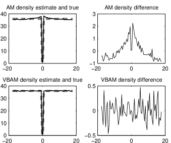
Figure 1: Left column: the upper plot is the adaptive Metropolis (AM) density and the lower plot is the variational Bayesian adaptive Metropolis (VBAM) density. The dashed line shows the true density while the black line shows the approximated density from samples. Right column: the upper plot shows the AM density difference between the true and approximated densities while the lower plot shows the density difference for the VBAM method. The density difference for the VBAM algorithm fluctuates around zero while the AM density difference does not. Therefore VBAM algorithm performs better than AM.

To compare the performance of AM and VBAM algorithms, we generated $10^{6}$ samples from each algorithm. As in Haario et al. [21], the comparison is done through computing the density differences of each method and the results are shown in Figure 1. The left column plots show the empirical densities produced by the adaptive Metropolis (AM) algorithm and the proposed variational Bayesian adaptive Metropolis (VBAM) algorithm, respectively. The right column shows, for each method, the difference between the real target density and the empirical densities. The VBAM algorithm indeed seems to give samples that follow well the true distribution, that is, the empirical density approximates well the true density. Because the density differences are around zero the results show the VBAM algorithm performs better than the AM algorithm.

5.2 100-dimensional Gaussian target distribution

In this example, we consider a high-dimensional Gaussian target distribution as discussed by Roberts and Rosenthal [31]. Here, the target distribution is $\mathbb{N}(0,MM^{T})$, where the entries of the $d\times d$ matrix $M$ are generated from unit Gaussian distributions [31]. We compare our results with a version of the AM algorithm considered in the article using the C-language implementation (adaptchol.c) provided by the authors. For the experiment we also implemented a C-language version of our VBAM adaptation so that the only difference in the runs is the covariance adaptation.

In the AM algorithm of Roberts and Rosenthal [31], at iteration $k$, the proposal distribution is defined as

$$q_{k}(\theta_{*}\mid\theta)=\begin{cases}\mathbb{N}\left(\theta,\frac{0.1^{2}}{d}\mathbf{I}\right),&\text{if $k\leq 2d$},\\ (1-\beta)\,\mathbb{N}\left(\theta,\frac{2.38^{2}}{d}\boldsymbol{\Sigma}_{k}\right)+\beta\,\mathbb{N}\left(\theta,\frac{0.1^{2}}{d}\mathbf{I}\right),&\text{if $k>2d$},\end{cases}$$ (28)

where $\boldsymbol{\Sigma}_{k}$ is the current empirical covariance and $\beta$ is a small positive constant. In the numerical experiment, we chose the dimensionality to be $d=100$ and $\beta=0.05$ following Roberts and Rosenthal [31]. For the VBAM algorithm, the state space model used is the Gaussian random walk model (27) with $\mathbf{A}=\mathbf{I}$, $\mathbf{H}=\mathbf{I}$, and $\mathbf{Q}=10^{-9}\,\mathbf{I}$, and $\lambda_{k}$ is updated using Equation (7). We initialized $\lambda_{0}=2.38^{2}/2$, the value of $\overline{\alpha}$ was 0.234 and we used the following $\gamma_{k}$ [26]:

$$\gamma_{k}\,=\,\frac{k_{0}}{\max\{k_{0},k^{\tau}\}},$$

where $k_{0}>1$ is the pre-specified value and $\tau\in(1/2\,,\,1]$. The used values for $k_{0}$ and $\tau$ were 1000 and 0.99, respectively.

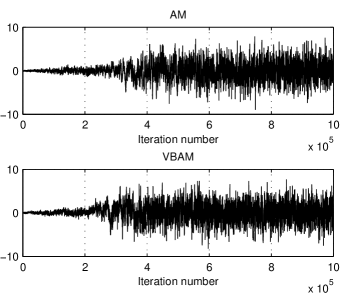
Figure 2: First coordinate of the MCMC chains in the 100-dimensional Gaussian target distribution example.

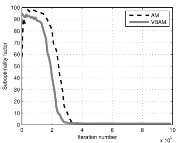
Figure 3: Suboptimality factors in the Gaussian target distribution example.

Trace plots of the first coordinate of the AM and VBAM chains are shown in Figure 2. It can be seen that the VBAM seems to stabilize to the stationary distribution a bit faster than the AM algorithm. This is confirmed by the suboptimality factors [31] shown in Figure 3. In this examples, the suboptimality factor of VBAM reaches the value of around one faster than AM which implies that its adaptation works faster.

5.3 20-dimensional banana-shaped distribution

In this example, we consider a banana-shaped distribution which is also often used as an example to study the performance of adaptive MCMC algorithms [20, 31, 21, 9]. The banana-shaped distribution density function is given as

$$\mathbf{f}(x_{1},x_{2},\ldots,x_{d}) \propto\exp\left(-\frac{x_{1}^{2}}{200}-\frac{1}{2}(x_{2}+B\,x_{1}^{2}-100\,B)^{2}-\frac{1}{2}(x_{3}^{2}+x_{4}^{2}+\cdots+x_{d}^{2})\right),$$

where $B>0$ is the ‘bananicity’ constant.

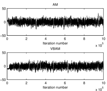
Figure 4: Trace plots of the first component of the banana distribution. The first row is the AM plot and the second is for VBAM. The mixing of the samples in both AM and VBAM is good.

We used the VBAM algorithm to sample from this distribution and compared the results with the AM algorithm of Roberts and Rosenthal [29] whose proposal distribution was (28). The VBAM state space model was the random walk model (27) with $\mathbf{A}=\mathbf{I}$, $\mathbf{H}=\mathbf{I}$ and $\mathbf{Q}=10^{-9}\,\mathbf{I}$. As in [29], we set $d=20$ and $B=0.1$ and ran the AM and VBAM algorithms for $10^{6}$ iterations. Figure 4 shows the trace plots for the first components $x_{1}$ and $x_{2}$. It can be observed that the AM and VBAM algorithms both mix with an approximately same speed.

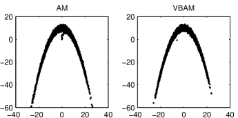
Figure 5: Scatter plots for the first two components in the banana example. The first plot is for AM, the second plot is for VBAM.

Figure 5 shows the scatter plots for AM and VBAM algorithms. As can be seen, the shapes of the plots indeed have a banana-like shape and they cover the support of the distribution well. In this example we did not find any significant difference between AM and VBAM, but still it shows that also the VBAM algorithm works well in this challenging sampling problem.

5.4 Chemical Reaction Model

As the first real data example we analyze a chemical reaction model studied in the book by Himmelblau [22]. The model found on page 326–327 [22] is a result of deterministic modeling of chemical reactions which involve six species ($A$, $B$, $C$, $D$, $E$ and $F$) and three type of reactions.

The chemical reactions are

$$\begin{split}A+B&\xrightarrow{k_{1}}C+F,\\ A+C&\xrightarrow{k_{2}}D+F,\\ A+D&\xrightarrow{k_{3}}E+F,\end{split}$$ (29)

and they are modeled with the differential equations

$$\begin{split}\frac{\mathrm{d}A}{\mathrm{d}t}&=-k_{1}A\,B-k_{2}A\,C-k_{3}A\,D,\\ \frac{\mathrm{d}B}{\mathrm{d}t}&=-k_{1}A\,B,\\ \frac{\mathrm{d}C}{\mathrm{d}t}&=k_{1}A\,B-k_{2}A\,C,\\ \frac{\mathrm{d}D}{\mathrm{d}t}&=k_{2}A\,C-k_{3}A\,D,\\ \frac{\mathrm{d}E}{\mathrm{d}t}&=k_{3}A\,D.\end{split}$$ (30)

The task is to estimate the parameters $k_{1}$, $k_{2}$ and $k_{3}$ from experimental data having the initial values given as $C(0)=D(0)=0$, $A(0)=0.02090\text{ mol/l}$ and $B(0)=A(0)/3$. The data are shown in Figure 6.

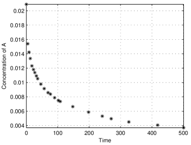
Figure 6: Experimental data for concentration of $A$ in the chemical reaction model.

The reported parameter values were $k_{1}=14.7$, $k_{2}=1.53$ and $k_{3}=0.294$ [22]. We applied the VBAM algorithm to sample the parameters and then compared the results with the reported ones. We used the random walk state space model (27) with $\mathbf{A}_{k}=\mathbf{I}$, $\mathbf{H}_{k}=\mathbf{I}$ and $\mathbf{Q}_{k}=10^{-9}\mathbf{I}$.

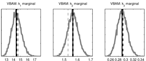
Figure 7: Marginal distributions for parameters $k_{1}$, $k_{2}$, and $k_{3}$ in the chemical reaction model estimated from the samples of VBAM plotted together with the sample means, maximum a posterior (MAP) estimates, and reported parameter values (RPV) in the chemical reaction model. Here, the gray lines denote the distributions, the black dotted lines the sample means, the light dotted lines the RPV, and the black lines the MAP estimates.

The marginal distribution plots estimated from 100,000 VBAM samples are shown in Figure 7. In the figure, it can be seen that the estimates are well consistent with the reported parameter values. The scatter plots for VBAM samples are shown in Figure 8. It is observed that there exist correlation between parameters, for example, $k_{2}$ and $k_{3}$ seems to have negative correlation. However, the correlation is not particularly strong and hence the parameters are quite well identifiable from the data.

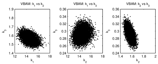
Figure 8: VBAM scatter plots for the chemical reaction model. It is observed that there is some correlation between the parameters.

5.5 Monod Model

As the second real data example, we analyze the bacteria growth models studied in the book by Berthouex and Brown [8]. The estimation of the parameters of the Monod model has been studied for instance, in Chapter 35 of the book [8], where the authors used the experimental data shown in Figure 9. The data were obtained by operating a continuous flow biological reactor at steady-state conditions and the following Monod model was proposed to fit the data:

$$y=\frac{\theta_{1}\,x}{\theta_{2}+x}+\epsilon.$$ (31)

In Equation (31), $y$ is the growth rate expressed per hour and is obtained at substrate concentration $x$, $\theta_{1}$ is the maximum growth rate expressed per hour, $\theta_{2}$ is the saturation constant, and $\epsilon$ is a Gaussian noise [8]. In [8], the parameters were estimated to be $\theta_{1}=0.153$ and $\theta_{2}=55.4$.

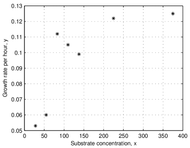
Figure 9: Data for the bacteria growth (Monod) model.

We estimated these parameters using the VBAM algorithm. We used the random walk state space model (27) for VBAM algorithm, where $\mathbf{A}_{k}=\mathbf{I}$, $\mathbf{H}_{k}=\mathbf{I}$ and $\mathbf{Q}_{k}=10^{-9}\mathbf{I}$.

The marginal distribution estimates computed from 100,000 VBAM samples together with the sample means, MAP estimates, and reported parameter values as well as the scatter plot are shown Figure 10. The plots show that the reported parameter values are well within the estimated parameter distribution and that there exist strong correlation between the parameters.

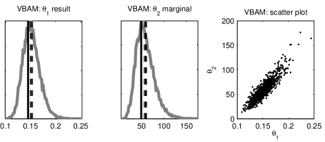
Figure 10: The first two plots from left show the marginal distributions for parameters $\theta_{1}$ and $\theta_{2}$ in the Monod model estimated from the samples of VBAM, plotted along with the sample means, MAP, and reported parameter values (RPV). The gray lines denote the distributions, the black dotted lines the sample means, the light dotted lines the RPV, and the black lines the MAP estimates. As can be seen, the parameter estimates are consistent with RPV. The plot on the right shows the scatter plot. The parameters $\theta_{1}$ and $\theta_{2}$ seem to have a strong positive correlation.

6 Conclusion and Discussion

In this paper, we have proposed a new adaptive Markov chain Monte Carlo (MCMC) method called variational Bayesian adaptive Metropolis (VBAM) algorithm, which adapts the covariance matrix of the Gaussian proposal distribution in the Metropolis algorithm with the variational Bayesian adaptive Kalman filter (VB-AKF, [34]). We have shown that the method is indeed a valid adaptive MCMC method in the sense that it samples from the correct target distribution by proving a strong law of large numbers for it. We have numerically tested the performance of the method in widely used example models and compared it to two other adaptive MCMC schemes. In the first two simulated experiments, our method turned out to perform better than the AM algorithm of Haario et al. [20, 21]. In the third simulated example, the performance was similar to the performance of the AM algorithm of Roberts and Rosenthal [29]. In the two real data examples, VBAM also produced results which are consistent with results reported in literature.

The advantage of the proposed method is that it has more parameters to tune, which gives more freedom. In particular, the tight relationship with the linear systems theory and Kalman filtering allows one to borrow good state space models from target tracking literature [24, 7] and use them as the models in VBAM. The correctness of the method can be easily verified by checking that the resulting state space model is uniformly completely observable and controllable, which is a standard step in building state space models. Sometimes, however, the freedom of choosing algorithm parameters can be seen as a disadvantage, because manual tuning of the VB-AKF model parameters can turn out to be challenging. Fortunately, in many cases a simple Gaussian random-walk state space model is a good default choice.

The computational requirements of the VBAM method are typically $O(d^{3})$, where $d$ is the parameter dimensionality, while the complexity of a usual implementation of AM is $O(d^{2})$. This is because the VB-AKF step is needed, which amounts to a (constant) number of Kalman filter updates at each iteration and these operations are computationally more demanding than what is needed in the standard AM. However, these operations are still quite cheap and when the model is complex enough to require MCMC sampling, the evaluation of the distribution can be expected to dominate the computation time anyway. Furthermore, these operations can be typically optimized for a given state space model. For example, in the random walk model we do not actually need to perform all the matrix operations in full generality, because the model matrices are diagonal. Even though the basic implementation of the method is straightforward and not significantly harder than implementation of an AM algorithm, developing an optimized version of the VBAM method for a particular type of state space model can be more complicated.

An advantage of the method is that it can also easily be generalized in various ways. For example, we could extend it by replacing the linear Kalman filter with non-linear Kalman filters such as the extended Kalman filter, a sigma-point (unscented) filter, or even particle filters [33]. In fact, provided that we can ensure that the mean and covariance of the corresponding non-linear Kalman filter remain bounded, replacing the linear VB-AKF with a non-linear one [34] should lead to a valid VBAM algorithm as well. Similarly, a (Rao–Blackwellized) particle filter could be used for estimating the noise covariance [33] and provided that the adaptation can be shown to diminish in time. However, with non-linear state space model it will be hard to find good state space models for the algorithm. This path is interesting though, because it can lead to a completely new family of adaptive MCMC algorithms, which utilize different kinds of filters in the proposal adaptation.

References

- Andrieu and Moulines [2006] C. Andrieu, E. Moulines, On the ergodicity properties of some adaptive MCMC algorithms, The Annals of Applied Probability 16 (2006) 1462–1505.
- Andrieu and Thoms [2008] C. Andrieu, J. Thoms, A tutorial on adaptive MCMC, Statistics and Computing 18 (2008) 343–373.
- Atchadé and Fort [2010] Y. Atchadé, G. Fort, Limit theorems for some adaptive MCMC algorithms with subgeometric kernels, Bernoulli 16 (2010) 116–154.
- Atchadé and Rosenthal [2005] Y. Atchadé, J.S. Rosenthal, On adaptive Markov chain Monte Carlo algorithms, Bernoulli 11 (2005) 815–828.
- Bai [2009] Y. Bai, Convergence of adaptive Markov chain Monte Carlo algorithms, Doctoral dissertation, University of Toronto, 2009.
- Bai et al. [2011] Y. Bai, G.O. Roberts, J.S. Rosenthal, On the containment condition for adaptive Markov chain Monte Carlo algorithms, Advances and Applications in Statistics 21 (2011) 1–54.
- Bar-Shalom et al. [2004] Y. Bar-Shalom, X.R. Li, T. Kirubarajan, Estimation with Applications to Tracking and Navigation: Theory, Algorithms and Software, John Wiley & Sons, 2004.
- Berthouex and Brown [2002] P.M. Berthouex, L.C. Brown, Statistics for Environmental Engineers, 2nd ed., CRC Press, 2002.
- Bornkamp [2011] B. Bornkamp, Approximating probability densities by iterated Laplace approximations, Computational and Graphical Statistics 20 (2011).
- Brooks et al. [2011] S. Brooks, A. Gelman, G. Jones, X. Meng, Handbook of Markov Chain Monte Carlo, Chapman Hall/CRC, 2011.
- Cai et al. [2006] B. Cai, R. Meyer, F. Perron, Metropolis–Hastings algorithms with adaptive proposals, Statistics and Computing 18 (2006) 421–433.
- Fort et al. [2011] G. Fort, E. Moulines, P. Priouret, Convergence of adaptive and interacting Markov chain Monte Carlo algorithms, The Annals of Statistics 39 (2011) 3262–3289.
- Gelman et al. [2013] A. Gelman, J.B. Carlin, H.S. Stern, D.B. Dunson, A. Vehtari, D.B. Rubin, Bayesian Data Analysis, 3rd ed., Chapman & Hall/CRC Press, 2013.
- Gelman et al. [1996] A. Gelman, G.O. Roberts, W.R. Gilks, Efficient Metropolis jumping rules, Bayesian Statistics 5 (1996) 599–607.
- Gilks et al. [1996] W.R. Gilks, S. Richardson, D.J. Spiegelhalter, Markov Chain Monte Carlo in Practice, Chapman & Hall/CRC Press, 1996.
- Gilks et al. [1994] W.R. Gilks, G.O. Roberts, E.I. George, Adaptive direction sampling, The Statistician 43 (1994) 179–189.
- Gilks et al. [1998] W.R. Gilks, G.O. Roberts, S.K. Sahu, Adaptive Markov chain Monte Carlo through regeneration, Journal of the American Statistical Association 93 (1998) 1045–1054.
- Griffin and Walker [2013] J.E. Griffin, S.G. Walker, On adaptive Metropolis–Hastings methods, Statistics and Computing 23 (2013) 123–134.
- Haario et al. [2006] H. Haario, M. Laine, A. Mira, E. Saksman, DRAM: efficient adaptive MCMC, Statistics and Computing 16 (2006) 339–354.
- Haario et al. [1999] H. Haario, E. Saksman, J. Tamminen, Adaptive proposal distribution for random walk Metropolis algorithm, Computational Statistics 14 (1999) 375–396.
- Haario et al. [2001] H. Haario, E. Saksman, J. Tamminen, An adaptive Metropolis algorithm, Bernoulli 7 (2001) 223–242.
- Himmelblau [1970] D.M. Himmelblau, Process Analysis by Statistical Methods, John Wiley & Sons, 1970.
- Holden et al. [2009] L. Holden, R. Hauge, M. Holden, Adaptive independent Metropolis–Hastings, The Annals of Applied Probability 19 (2009) 395–413.
- Jazwinski [1970] A.H. Jazwinski, Stochastic Processes and Filtering Theory, Academic Press, 1970.
- Kalman [1960] R.E. Kalman, A new approach to linear filtering and prediction problems, Journal of Basic Engineering 82 (1960) 35–45.
- Liang et al. [2010] F. Liang, C. Liu, R.J. Carroll, Advanced Markov Chain Monte Carlo Methods: Learning from Past Samples, John Wiley & Sons, 2010.
- Luenberger and Ye [2008] D.G. Luenberger, Y. Ye, Linear and Nonlinear Programming, 3rd ed., Springer, 2008.
- Ren et al. [2008] Y. Ren, Y. Ding, F. Liang, Adaptive evolutionary Monte Carlo algorithm for optimization with applications to sensor placement problems, Statistics and Computing 18 (2008) 375–390.
- Roberts and Rosenthal [2001] G.O. Roberts, J.S. Rosenthal, Optimal scaling for various Metropolis–Hastings algorithms, Statistical Science 16 (2001) 351–367.
- Roberts and Rosenthal [2007] G.O. Roberts, J.S. Rosenthal, Coupling and ergodicity of adaptive Markov chain Monte Carlo algorithms, Journal of Applied probability 44 (2007) 458–475.
- Roberts and Rosenthal [2009] G.O. Roberts, J.S. Rosenthal, Examples of adaptive MCMC, Journal of Computational and Graphical Statistics 18 (2009) 349–367.
- Saksman and Vihola [2010] E. Saksman, M. Vihola, On the ergodicity of the adaptive Metropolis algorithm on unbounded domains, The Annals of applied probability 20 (2010) 2178–2203.
- Särkkä [2013] S. Särkkä, Bayesian Filtering and Smoothing, Cambridge University Press, 2013.
- Särkkä and Hartikainen [2013] S. Särkkä, J. Hartikainen, Non-linear noise adaptive Kalman filtering via variational Bayes, in: Proceedings of MLSP 2013, pp. 1–6.
- Särkkä and Nummenmaa [2009] S. Särkkä, A. Nummenmaa, Recursive noise adaptive Kalman filtering by variational Bayesian approximations, IEEE Transactions on Automatic Control 54 (2009) 596–600.
- Vihola [2011] M. Vihola, On the stability and ergodicity of adaptive scaling Metropolis algorithms, Stochastic Processes and their Applications 121 (2011) 2839–2860.
- Vihola [2012] M. Vihola, Robust adaptive Metropolis algorithm with coerced acceptance rate, Statistics and Computing 22 (2012) 997–1008.
- Vrugt and Braak [2011] J.A. Vrugt, C.J.T. Braak, DREAM(D): an adaptive Markov chain Monte Carlo simulation algorithm to solve discrete, noncontinuous, and combinatorial posterior parameter estimation problems, Hydrology and Earth System Sciences 15 (2011) 3701–3713.
- Vrugt et al. [2009] J.A. Vrugt, C.J.T. Braak, C. Diks, B.A. Robinson, J.M. Hyman, D. Higdon, Accelerating Markov chain Monte Carlo simulation by differential evolution with self-adaptive randomized subspace sampling, International Journal of Nonlinear Sciences and Numerical Simulation 10 (2009) 273–290.