Computing 1-D atomic densities in macromolecular simulations: the Density Profile Tool for VMD

Abstract

Molecular dynamics simulations have a prominent role in biophysics and drug discovery due to the atomistic information they provide on the structure, energetics and dynamics of biomolecules. Specialized software packages are required to analyze simulated trajectories, either interactively or via scripts, to derive quantities of interest and provide insight for further experiments. This paper presents the Density Profile Tool, a package that enhances the Visual Molecular Dynamics environment with the ability to interactively compute and visualize 1-D projections of various density functions of molecular models. We describe how the plugin is used to perform computations both via a graphical interface and programmatically. Results are presented for realistic examples, all-atom bilayer models, showing how mass and electron densities readily provide measurements such as membrane thickness, location of structural elements, and how they compare to X-ray diffraction experiments.

Program summary

Manuscript Title: Computing 1-D atomic densities in macromolecular simulations: the Density Profile Tool for VMD
Authors: Toni Giorgino
Program Title: Density Profile Tool
Journal Reference:
Catalogue identifier:
Licensing provisions: 3-clause BSD Open Source.
Programming language: TCL/TK.
Computer: Any, with or without graphical display.
Operating system: Linux/Unix, OSX, Windows.
RAM: VMD should be able to hold the trajectory in memory.
Number of processors used: 1
Keywords: Electron density, projection, bilayer, cholesterol, lipid, phospholipid, membrane, trajectory, structural biology, graphical user interface, GUI, computational, molecular graphics
Classification: 3 Biology and Molecular Biology, 23 Statistical Physics and Thermodynamics.
External routines/libraries: VMD (version 1.9 or higher).
Nature of problem: Compute and visualize one-dimensional density profiles of molecular dynamics trajectories in the VMD environment, either interactively or programmatically.
Solution method: Density profiles are computed by binning the simulation space into slabs of finite thickness. A graphical user interface allows to choose the atomic property (number, mass, charge, electrons) and the details of the binning.
Restrictions: The current version only supports orthorhombic cells.
Unusual features: The Density Profile Tool is not a standalone program but a plug-in that enhances VMD’s analysis features.
Running time: A contemporary PC completes the analysis of 500 frames of the example system discussed in the paper (35,000 atoms) in under 1 min.

1 Introduction

Molecular dynamics (MD) is a compute-intensive technique that simulates the evolution of a system on the basis of interatomic forces and Newton’s laws of motion. MD has become a popular and successful methodology to investigate the behavior of biomolecular systems at an atomistic scale, because it provides structural information at temporal and spatial resolutions much finer than those afforded by most experimental techniques [1, 2]. Studies routinely use MD to probe the behavior of systems as diverse as solvated globular proteins, biological membranes [3], transmembrane proteins [4], receptor domains [5, 6], drug-protein interactions [7, 8], etc. Predictivity is ensured by empirical force-fields which undergo periodic refinements in order to faithfully reproduce structural, energetic and kinetic observables [9].

Density functions, such as number or mass densities, is one of the observables that can be derived from MD trajectories. For planar systems, like biological membranes, it is convenient to project density functions along the plane’s normal to obtain 1-D profiles (Figure 1). The profiles can be connected to experimental observables; for example, the distance between peaks of lipid’s phosphate groups is a direct indicator of bilayer thicknesses, while electron density profiles are related to low angle diffraction and scattering data [10].

This paper describes the Density Profile tool, a software package that computes one-dimensional density profiles of molecular systems. The software is used from within the open-source Visual Molecular Dynamics (VMD) environment, leveraging its extensive support for file formats, interactive graphical display, atom selection syntax, etc. [11] The plugin provides both a graphical user interface (GUI), which makes it immediate to setup computations, and a scripting interface. GUI usage is generally convenient to perform casual inspections, because no learning curve is involved; on the other hand, the integration with VMD’s scripting environment, based on the TCL language [12], makes it possible to embed calculations in more complex protocols and build on its results.

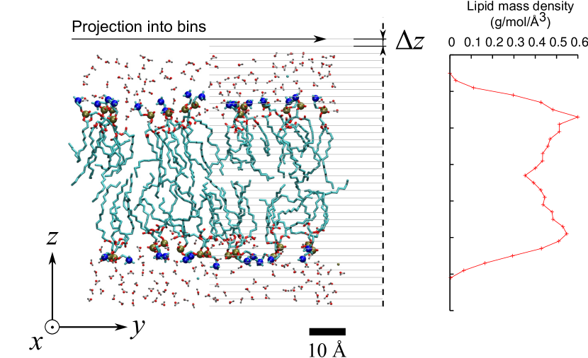
Figure 1: Left: computation of the density profile of a lipid bilayer whose normal is parallel to the $z$ axis. Profile resolution is $\Delta z=2$ Å. Right: mass density profile computed for lipid molecules.

1.1 Related work

Other analysis packages contain command-line tools to perform density profile computations similar to the one described here. GROMACS’ distribution, for example, provides g_density, a stand-alone executable meant to be used from the command-line or in shell scripts [13]. This approach has the advantage of not being tied to a specific graphical or scripting environment; however, it can be limiting in three respects: first, a GUI may be desirable for quick one-off computations; second, binaries mostly require GROMACS-specific file formats and topologies; finally, performing computations in shell scripts implies a programming model in which text files are used to store intermediate results – a model which is more cumbersome than manipulating variables, the route afforded by conventional programming languages like TCL or Python.

2 Computational methods

Assuming point-like atoms (an assumption generally justified in classical MD, see section 3.4), the algorithm to compute density profiles is straightforward. For the sake of clarity, here we assume to be interested in the mass density profile along the $z$ axis, with a granularity of $\Delta z$.

First, the space is divided in equally-sized slabs of thickness $\Delta z$. Assuming orthorhombic periodic boundary conditions (PBC), the slabs will extend in the $xy$ plane up to the boundaries of the unit cell; otherwise, they can be considered infinitely large. Slabs are indexed by a (relative) integer $b$; slab $b$ will include the spatial region $b\Delta z\leq z<(b+1)\Delta z$ (Figure 2). Defining the indicator function $\delta_{b}(z)$ for slab $b$,

$$\delta_{b}(z)=\left\{\begin{array}[]{rl}1&\mbox{if $b\leq z/\Delta z<b+1$}\\ 0&\mbox{otherwise}\end{array}\right.$$

the value of the density function at bin $b$ is obtained by binning the chosen atomic property $p_{i}$, then normalizing by the slab volume:

$$\rho_{b}=(L_{x}L_{y}\Delta z)^{-1}\sum_{i\in\mathrm{atoms}}\delta_{b}(z_{i})p_{i}$$ (1)

where $L_{x}$ and $L_{y}$ are the sides of the periodic cell, $z_{i}$ is the $z$ coordinate of the center of atom $i$. In the case of an infinite system, it is possible to assume $L_{x}=L_{y}=1$ and obtain linear (as opposed to volumetric) density values along $z$.

Depending on whether number, mass, charge or electron number density is to be computed, the value of $p_{i}$ is taken from different atomic attributes, according to Table 1. These properties are generally stored in the MD topology file associated with the system.

Density function	$p=$
Number	1
Mass	$m_{a}$
Charge	$q$
Electron number	$Z-q$
Electron number (neutral)	$Z$

Table 1: Supported density function types and the corresponding value to be used for $p_{i}$ in Eq. (1). $m_{a}$ is the atomic mass, $q$ the partial charge, $Z$ the atomic number. In classical MD these properties can be derived from topology files, the atom’s name, and/or its type.

Figure 2: Arrangement of the volume slabs in a periodic cell. Density is being computed along the $z$ axis with a resolution of $\Delta z$. Bin $b$ (integer) contains atoms whose $z$ coordinate satisfies $b\leq z/\Delta z<(b+1)$; each slab has a volume of $L_{x}L_{y}\Delta z$.

3 Program description

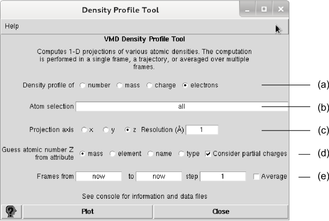
Figure 3: The plugin’s graphical interface. Clicking the “Plot” button starts the computation and shows the results in a plot window, with the option of exporting them as tabular data files. Labels are referenced in the main text.

3.1 Graphical user interface

The most direct way to perform density profile calculations is to load the trajectory to be analyzed in VMD and open the plugin’s GUI via the Extensions–Analysis menu entry. A window will appear (Figure 3) and offer the chance to set the analysis parameters, with sensible defaults.

The GUI is meant to be self-explanatory. The user is able to select the property whose density is to be computed (Figure 3, a); the subset of the atoms to consider (b); and the projection axis and bin size (c). Atom subsets are specified through VMD’s high-level atom selection syntax, which allows complex queries on the base of geometry, atom types, structural elements, and so on.

In case of electron density computations, we remark that topology files generally do not store the required atomic number $Z$. Therefore, an option (d) is provided to infer $Z$ from other atomic properties, such as masses, names, or types (the former being the most reliable). The heuristics to obtain $Z$ are provided by the TopoTools package [14]. The consider partial charges option includes or excludes partial charges from the electron density.

Finally, a subset of the trajectory frames can be selected for analysis setting an interval and stride (e). If the average option is enabled, average and standard deviations of densities over the chosen trajectory interval will be reported; otherwise, the selected frames are analyzed individually.

The analysis is started by clicking Plot button, after which results will appear in a plot window. The plot’s Export menu allows to save the graph itself or tabular ASCII data for further processing.

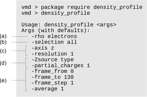
Figure 4: Command line interface for the density profile calculation function (with default values; 130 is the last loaded frame). Labels indicate the matching GUI controls in Figure 3.

3.2 Command line interface

Although the GUI makes it immediate to inspect density profiles of the currently loaded trajectory, in practice the need often arises to analyze series of simulations, or to use the results in a more complicated analysis protocol. For these reasons, all of the plugin’s functions can also be accessed through a command-line interface, after loading the package with the package require density_profile syntax.

The tool’s computations can be used in analysis programs written in TCL (VMD’s embedded language) via the density_profile function. Calling the function without arguments prints an usage summary on the console, with a list of options and their defaults (Figure 4). The options mirror the controls provided by the GUI; for example, the -rho argument takes one of the number, mass, charge or electrons keywords; when computing electron densities, -Zsource should be either mass, element, name or type.

Invoking the function performs the calculation on the currently loaded system and returns two TCL lists, each containing as many elements as there are bins. The first list holds the density values of each bin; the second list contains the corresponding lower coordinates, i.e. the locations of bin breaks. If only one frame is selected, or the “average” option is enabled, the density values are scalar values (one density value is returned per bin). If multiple frames are selected (via the -frame_from, _to, and _step parameters), density values will themselves be lists, holding results per bin and frame (see example in Section 4.1).

Provision of a double interface (mouse- and command-line driven) is consistent with the rest of the VMD environment. The ability to use plugins programmatically and to combine them into scripts is one of the strengths of VMD, which enables the construction of arbitrarily complex protocols.

3.3 Units of measurement

	Unit cell
Function	set	not set
Number density	Å-3	Å-1
Mass density	Da/Å3	Da/Å
Charge density	e/Å3	e/Å
Electron density	Å-3	Å-1

Table 2: Units of measurement of the computed densities. Unit Å is $10^{-10}$ m; Da is one dalton, or unified atomic mass unit, equal to 1 g/mol $\simeq 1.66\times 10^{-27}$ Kg; e $\simeq 1.60\times 10^{-19}$ coulomb is one elementary charge.

The behaviour of the plugin differs depending on whether the size of the periodic cell is available or not. In the former case, the real-space volume of each slab is known, and the plugin computes the expected volumetric densities (Figure 2), normalized by cubic Ångström. Following VMD’s conventions, the units of measurements used are atoms (number density), Dalton (mass), elementary charges (charge) or electron number, as per Table 2.

If the volume of the unit cell is not known, or the simulation was performed without PBC, the plugin will normalize densities with respect to the bin width, thus reporting densities per unit of length. Linear densities can then be normalized manually (which can be useful e.g.  to deal with non-orthorhombic cells).

3.4 Limitations

The algorithm considers point-like atoms instead of volumetric distributions; the tool would therefore be inappropriate to compute the density of isolated atoms with sub-Å resolution (a setup generally outside the scope of MD). The point-like atom approximation is valid as long as the chosen resolution is coarser than the average atomic radius, or the number of atoms in each bin is large. The latter condition is commonly satisfied in the MD practice.

The current version of the package restricts simulations to those performed in orthorhombic boundary conditions (either constant or variable boxes). It should be noted that these are the conditions used in most contemporary large-scale MD simulations [15, 16].

Finally, the plugin should provide correct results on coarse-grained and united-atom models [17], such as the Martini force-field [18], as well; this is due to the fact that the coarse-grained topologies often contain the correct atomic properties, with the exception of atomic numbers. For electron density computations, “united” atomic numbers for the various atoms types should be set manually (e.g. 10 for an united-atom water molecule), because the heuristics to deduce atomic numbers is based on all-atom systems.

4 Examples

To illustrate the use of density profiles with a realistic use case, we equilibrated a model bilayer of 1-palmitoyl-2-oleoyl-sn-glycero-3-phosphocholine (POPC) lipids in presence and absence of cholesterol in a 4:1 ratio. The hydrated membrane systems were constructed with the CHARMM-GUI membrane builder interface [19, 20], using a symmetric composition for the two leaflets, 70 Å initial box size, 15 Å water buffer per side, and 0.15 M KCl ionic strength. The generated systems, containing approximately 35,000 atoms each, were parametrized with the CHARMM36 lipid forcefield [21] (cross-section shown in Figure 1). After 1000 steps of conjugate-gradient minimization, systems were simulated with the ACEMD software [22] for 100 ns in the constant-pressure (NPT) ensemble, holding fixed the $x$-$y$ aspect ratio of the periodic box.

Density profiles were computed considering the last 50 ns of each trajectory, using snapshots taken every 100 ps (500 frames per simulation). Figure 5 (a) compares the final mass distributions of POPC molecules of the two systems, shown as average and standard deviations along the analysis interval. As expected, the bulky cholesterol molecules contribute to the membrane surface area interposing between POPC molecules; therefore, POPC volumetric mass density is decreased by approximately 15%

Second, we computed the electron density of a pure 1,2-dioleoyl-sn-glycero-3-phosphocholine (DOPC) lipid bilayer, prepared as above, and compared it with the experimental profile determined through X-ray scattering by Gandhavadi et al. [23, Figure 5]. Figure 5 (b) shows that the experimental (solid line) and MD-derived profiles (points with standard deviations) are in excellent agreement. Analogously, Figure 5 (c) compares the computed profiles for a mixture of 2:1 DOPC-cholesterol (points) with the experimental results by Gandhavadi et al. (solid line) [23, Figure 7] and Hung et al. (dashed line) [24, Figure 5]; the agreement for this heterogeneous bilayer is very good, as well. Experimental profiles, originally in arbitrary units, were scaled to fit.

As a last example, Figures 5 (d,e) compare the mass and electron density profiles of a polyunsaturated fatty acid phospholipid bilayer (1,2-diarachidonoyl-glycero-3-phosphocholine, DAPC) and a saturated one (1,2-dimyristoyl-sn-glycero-3-phosphocholine, DMPC), both prepared as above. The profiles include phospholipids together with solvent; accordingly, the density values outside of the bilayer region converge towards the values expected for bulk water (dotted lines).

Figure 5: Density profiles in bilayer models. (a) Mass density distribution of POPC molecules in a pure-POPC bilayer (open squares) and a 4:1 POPC-cholesterol mixture (filled). (b) Electron density profiles of a pure-DOPC system: computed (squares) and experimentally-determined (solid line) [23, Fig. 5]. (c) Electron density profiles of a 2:1 DOPC-cholesterol system: computed (squares) and experimentally determined by Gandhavadi et al. [23, Fig. 7] and Hung et al. [24, Fig. 5]. (d, e) Computed mass and electron density profiles for a polyunsaturated (DAPC) and a saturated (DMPC) fatty-acid phospholipid bilayer; dotted lines indicate densities of bulk water.

4.1 Scripting

For the sake of illustration, we perform the same mass calculation of the above example, this time accessing the results through the customary VMD-TCL language syntax:

⬇

vmd > set dp [density_profile -rho mass -selection lipid

-frame_to 99 -frame_from 50 -frame_step 1]

vmd > puts [lindex $dp 0 3 5] # Meaning dp(0,3,5)

vmd > puts [lindex $dp 1 3]

The first line performs the mass density computation (without any graphical interaction). The return value of the function call, a list of two lists, is assigned to the variable dp. The next command prints the value of the density at bin 3 of the 6th selected frame (trajectory frame 55). Analogously, the last line extracts the fourth element of the second returned list, i.e. the lower coordinate of bin 3; lindex is TCL’s list index operator (indices are zero-based).

5 Compatibility and distribution

The density profile tool is written in TCL and is platform-independent; it will therefore work on any of the platforms supported by the VMD system, notably Linux, OSX, Windows, and numerous Unix variants [11].

The source is released under a 3-clause BSD license. The latest version of the package can be obtained from the URL multiscalelab.org/utilities/DensityProfileTool. The archive also contains cross-platform installation instructions.

6 Acknowledgments

Package development was started while at the Computational Biophysics Laboratory (GRIB-IMIM-UPF) of the Universitat Pompeu Fabra with partial support by the Agència de Gestió d’Ajuts Universitaris i de Recerca, Generalitat de Catalunya (2009 BP-B 00109). These institutions are gratefully acknowledged.

References

- Dror et al. [2012] R. O. Dror, R. M. Dirks, J. Grossman, H. Xu, D. E. Shaw, Biomolecular simulation: A computational microscope for molecular biology, Annual Review of Biophysics 41 (2012) 429–452.
- Harvey and De Fabritiis [2012] M. J. Harvey, G. De Fabritiis, High-throughput molecular dynamics: the powerful new tool for drug discovery, Drug Discovery Today 17 (2012) 1059–1062.
- Ash et al. [2004] W. L. Ash, M. R. Zlomislic, E. O. Oloo, D. P. Tieleman, Computer simulations of membrane proteins, Biochimica et Biophysica Acta (BBA) - Biomembranes 1666 (2004) 158–189.
- Dror et al. [2009] R. O. Dror, D. H. Arlow, D. W. Borhani, M. O. Jensen, S. Piana, D. E. Shaw, Identification of two distinct inactive conformations of the beta2-adrenergic receptor reconciles structural and biochemical observations, Proceedings of the National Academy of Sciences of the United States of America 106 (2009) 4689–4694.
- Ahmad et al. [2008] M. Ahmad, W. Gu, V. Helms, Mechanism of fast peptide recognition by SH3 domains, Angewandte Chemie (International Ed. in English) 47 (2008) 7626–7630.
- Giorgino et al. [2012] T. Giorgino, I. Buch, G. De Fabritiis, Visualizing the induced binding of SH2-Phosphopeptide, J. Chem. Theory Comput. 8 (2012) 1171–1175.
- Buch et al. [2011] I. Buch, T. Giorgino, G. De Fabritiis, Complete reconstruction of an enzyme-inhibitor binding process by molecular dynamics simulations, Proceedings of the National Academy of Sciences 108 (2011) 10184–10189.
- Shan et al. [2011] Y. Shan, E. T. Kim, M. P. Eastwood, R. O. Dror, M. A. Seeliger, D. E. Shaw, How does a drug molecule find its target binding site?, Journal of the American Chemical Society 133 (2011) 9181–9183.
- Beauchamp et al. [2012] K. A. Beauchamp, Y.-S. Lin, R. Das, V. S. Pande, Are protein force fields getting better? a systematic benchmark on 524 diverse NMR measurements, Journal of Chemical Theory and Computation 8 (2012) 1409–1414.
- Nagle and Wiener [1989] J. F. Nagle, M. C. Wiener, Relations for lipid bilayers. connection of electron density profiles to other structural quantities., Biophysical Journal 55 (1989) 309–313.
- Humphrey et al. [1996] W. Humphrey, A. Dalke, K. Schulten, VMD: visual molecular dynamics, J Mol Graph 14 (1996) 33–38.
- Ousterhout and Jones [2009] J. K. Ousterhout, K. Jones, Tcl and the Tk Toolkit, Addison-Wesley Professional, 2nd edition, 2009.
- Hess et al. [2008] B. Hess, C. Kutzner, D. van der Spoel, E. Lindahl, GROMACS 4: Algorithms for highly efficient, load-balanced, and scalable molecular simulation, Journal of Chemical Theory and Computation 4 (2008) 435–447.
- Kohlmeyer [2012] A. Kohlmeyer, TopoTools Plugin, Version 1.2, Accessed 7 May 2012. http://www.ks.uiuc.edu/Research/vmd/plugins/topotools/.
- Shaw et al. [2010] D. E. Shaw, P. Maragakis, K. Lindorff-Larsen, S. Piana, R. O. Dror, M. P. Eastwood, J. A. Bank, J. M. Jumper, J. K. Salmon, Y. Shan, W. Wriggers, Atomic-level characterization of the structural dynamics of proteins, Science 330 (2010) 341 –346.
- Buch et al. [2010] I. Buch, M. J. Harvey, T. Giorgino, D. P. Anderson, G. De Fabritiis, High-throughput all-atom molecular dynamics simulations using distributed computing, Journal of Chemical Information and Modeling 50 (2010) 397–403.
- Tozzini [2010] V. Tozzini, Minimalist models for proteins: a comparative analysis, Quarterly Reviews of Biophysics 43 (2010) 333–371.
- Monticelli et al. [2008] L. Monticelli, S. K. Kandasamy, X. Periole, R. G. Larson, D. P. Tieleman, S.-J. Marrink, The MARTINI coarse-grained force field: Extension to proteins, Journal of Chemical Theory and Computation 4 (2008) 819–834.
- Jo et al. [2009] S. Jo, J. B. Lim, J. B. Klauda, W. Im, CHARMM-GUI membrane builder for mixed bilayers and its application to yeast membranes, Biophysical Journal 97 (2009) 50–58.
- Jo et al. [2008] S. Jo, T. Kim, V. G. Iyer, W. Im, CHARMM-GUI: a web-based graphical user interface for CHARMM, Journal of Computational Chemistry 29 (2008) 1859–1865.
- Klauda et al. [2010] J. B. Klauda, R. M. Venable, J. A. Freites, J. W. O’Connor, D. J. Tobias, C. Mondragon-Ramirez, I. Vorobyov, A. D. MacKerell, R. W. Pastor, Update of the CHARMM all-atom additive force field for lipids: Validation on six lipid types, The Journal of Physical Chemistry B 114 (2010) 7830–7843.
- Harvey et al. [2009] M. J. Harvey, G. Giupponi, G. D. Fabritiis, ACEMD: accelerating biomolecular dynamics in the microsecond time scale, Journal of Chemical Theory and Computation 5 (2009) 1632–1639.
- Gandhavadi et al. [2002] M. Gandhavadi, D. Allende, A. Vidal, S. Simon, T. McIntosh, Structure, composition, and peptide binding properties of detergent soluble bilayers and detergent resistant rafts, Biophysical Journal 82 (2002) 1469–1482.
- Hung et al. [2007] W.-C. Hung, M.-T. Lee, F.-Y. Chen, H. W. Huang, The condensing effect of cholesterol in lipid bilayers, Biophysical Journal 92 (2007) 3960–3967.