Triangular Bose-Hubbard trimer as a minimal model for a superfluid circuit

Abstract

The triangular Bose-Hubbard trimer is topologically the minimal model for a BEC superfluid circuit. As a dynamical system of two coupled freedoms it has mixed phase-space with chaotic dynamics. We employ a semiclassical perspective to study triangular trimer physics beyond the conventional picture of the superfluid-to-insulator transition. From the analysis of the Peierls-Nabarro energy landscape, we deduce the various regimes in the $(\Omega,u)$ parameter-space, where $u$ is the interaction, and $\Omega$ is the superfluid rotation-velocity. We thus characterize the superfluid-stability and chaoticity of the many-body eigenstates throughout the Hilbert space.

I Introduction

The experimental study of Bose-Einstein Condensates (BECs) allows the realization of ultracold atomic superfluid circuits e1 ; e2 ; e3 ; e4 ; e5 ; e6 ; e7 ; e8 ; e9 ; e10 ; e11 ; e12 ; e13 ; e14 and the incorporation of a laser-induced weak-link (a bosonic Josephson junction) within them e15 . By rotating such a barrier it is possible to induce current Hekk and to drive phase-slips between quantized superfluid states of a low dimensional toroidal ring e15 . Such mesoscopic devices open a new arena for detailed study of complex Hamiltonian dynamics.

The hallmark of superfluidity is a stable non-equilibrium steady-state current. If $N$ bosons in a rotating ring are condensed into a single plane-wave orbital, one obtains a “vortex state” with a quantized current per particle ($I/N$) Udea ; Carr1 ; Carr2 ; Brand1 . For non-interacting bosons the lowest vortex-state is also the ground-state. It is stable and carries a microscopically small “persistent current”. By contrast, all higher vortex states are unstable. Interactions change the picture dramatically nir : the Bogolyubov-spectrum of the one-particle excitations of a vortex-state is modified (e.g. by the appearance of phonons), and hence all vortex-states that satisfy the Landau criterion Landau ; Hakim ; Leboeuf become stable. See Fig.​​ 1 for illustration, and Section VI for extra pedagogical details.

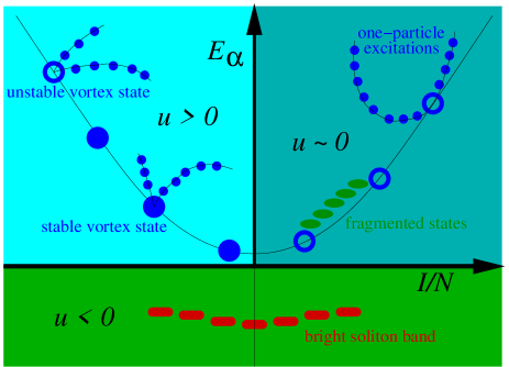
Figure 1: (Color online) Representative eigen-energies $E_{\alpha}$ of a rotating ring system are classified by the current $I$ they carry in the rotating frame of reference. The filled and hollow blue circles represent stable and unstable vortex-states for which $I/N$ is quantized. The blue dots represent their Bogolyubov one-particle excitations. On the upper right $u$ is vanishingly small, while on the upper left $u$ is large and positive, resulting in phonon branches. The green elliptic dots represent fragmented states (here the particles are divided between two vortex orbitals). For negative $u$ (lower plane) there are stable bright soliton solutions. Red oval dots represent eigenstates that are formed by superposition of such solitons. For positive $u$, and appropriate rotation frequency, one may observe additional type of eigenstates that are formed of dark solitons (not illustrated). Adding weak disorder, the unstable vortex-states would mix with their excitations, and the soliton band would decompose into a set of standing solitons.

The vortex-state of bosons in a ring constitutes one particular example of a coherent (non-fragmented) state. Other coherent-state solutions may correspond, for example, to all bosons condensed in a localized orbital (bright soliton) Udea , or in an orbital that has a notch (dark soliton) Carr1 ; Carr2 . From such non-stationary classical solutions one can superpose stationary quantum eigenstates whose angular momentum is not quantized.

The above picture is missing a central ingredient: there is no reference to the global structure of the underlying phase-space that dictates the dynamics. Vortex-states and solitons are minima or maxima of the energy landscape, and the Bogolyubov spectrum merely reflects the linear-stability analysis in the vicinity of these solutions. We are therefore motivated to consider the simplest paradigm for a superfluid circuit which still allows the thorough investigation of its phase-space structure. The natural choice for such a model is bosons in a one-dimensional ring as in Ref. Brand1 or its discrete $M$ site version, described by the Bose-Hubbard Hamiltonian (BHH) BHH1 ; BHH2 ; Ofir1 ; Ofir2 as in Ref. Altman .

The phase-space of the ring model was studied within a two-orbital approximation Brand2 . However, such an approximation is not a valid minimal model by itself. From a topological point of view the minimal model for a superfluid circuit has to involve $M{=}3$ sites: a triangular Bose-Hubbard trimer (this would be equivalent to three non-localized modes). A close relative is the linear Bose-Hubbard trimer. The trimer phase-space has been partially studied in several papers trimer1 ; trimer2 ; trimer3 ; trimer4 ; trimer5 ; trimer6 ; trimer7 ; trimer8 ; trimer9 ; trimer10 ; trimer11 ; trimer12 ; trimer13 , and has been recognized as a building block for studies of transport Henn1 ; Henn2 and mesoscopic thermalization KottosBoris ; trm .

In this work we study the triangular Bose-Hubbard trimer as a topologically minimal model for a BEC superfluid circuit. In particular, we note that the mixed phase-space aspect of the dynamics has far reaching consequences, producing non-trivial physics that goes beyond the conventional picture of the Mott superfluid-to-insulator transition. Our approach relies on the analysis of the Peierls-Nabarro energy landscape Henn1 ; Henn2 ; Kivshar93 ; Rumpf04 , from which we deduce various regimes in the $(\Omega,u)$ parameter-space of the triangular BHH trimer, where $u$ is the interaction parameter, and $\Omega$ is the superfluid rotation-velocity. In each of these regimes we outline the structure of phase-space and the classification of the many-body eigenstates. The criteria for the superfluid stability as opposed to chaoticity are thus determined.

(a)                                                      (b)
                   

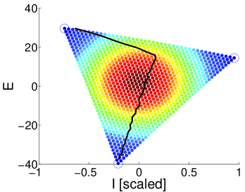
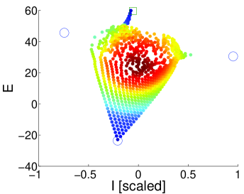
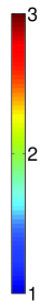
(c)                                                      (d)                                             (e)

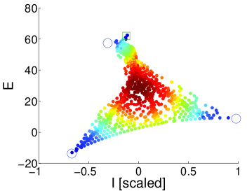
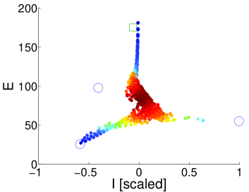
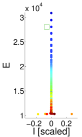
Figure 2: (Color online) The quantum spectrum of $N=42$ bosons in a triangular BEC trimer. Panels (a-e) are for ${(\Phi,u)}$ as follows: ${(0.2\pi,0.2)}$; ${(0.2\pi,2.5)}$; ${(0.7\pi,2.5)}$; ${(0.6\pi,8.5)}$; ${(0.6\pi,1470)}$. The units of time are such that $K{=}1$. Each point represents an eigenstate color-coded by its purity (blue $(1/S)\sim 1$ to red $(1/S)\sim 3$), and positioned according to its energy $E_{\alpha}$ and its scaled current $I_{\alpha}/(NK/M)$. The expected location of vortex-states, if they survive, is given by Eq.​​ (23) and Eq.​​ (11), and represented as empty blue circles. In panels (b-d), due to bifurcations, stable solitons are found in the expected semi-classical locations (indicated by empty green squares). In (c) as opposed to (b) the rotation frequency is large enough to stabilize an intermediate vortex-state. In (e) as opposed to (d) the interaction is strong, and the Mott transition of the ground-state is reflected in its low purity. The remaining low-purity fragmented states dwell in the chaotic sea and do not carry a quantized current. For large $M$ we expect their dispersion in $I$ to shrink further down compared with the quantized values. The thick black line in (a) is the microcanonical value of $I$.

II A rotating device

In a typical experimental scenario the potential is translated along the circuit, and can be written as ${V(\theta-\Omega t)}$. For theoretical analysis it is more convenient to transform the Hamiltonian to a rotating frame wherein the potential is time-independent. The rotation is thus formally equivalent to the introduction of a magnetic flux $\Phi$ through the ring. To relate the flux $\Phi$ to the rotation velocity $\Omega$ it is sufficient, without loss of generality, to write the one-particle Hamiltonian as follows:

$$\mathcal{H}\ \ = \ \ \frac{1}{2\mathsf{m}R^{2}}\left(p_{\theta}-\frac{\Phi}{2\pi}\right)^{2}+V(\theta)$$ (1)

$$\equiv \ \ \mathcal{H}_{0}-\Omega p_{\theta}+\mbox{const}~{},$$ (2)

where $R$ is the radius of the ring, $\theta$ is the angular position coordinate, and $p_{\theta}$ is the conjugate angular momentum. In the second equality $\mathcal{H}_{0}$ is defined as the Hamiltonian in the absence of magnetic flux. Consequently one observes that $\mathcal{H}$ is formally the same Hamiltonian as that of a rotating system with the implied identification

$$\Omega\ \ =\ \ \left[\frac{1}{\mathsf{m}R^{2}}\right]\frac{\Phi}{2\pi}~{}.$$ (3)

In references Udea ; Carr1 ; Carr2 units are set such that the pre-factor in the square brackets is unity. Hence, throughout this paper ${\Phi=2\pi}$ corresponds to ${\Omega=1}$ in these references.

We consider $V(\theta)$ consisting of $M$ deep wells, for which a tight-binding model is appropriate. The hopping frequency $K=1/(\mathsf{m}_{\text{eff}}a^{2})$ is conventionally expressed in terms of the lattice constant $a=2\pi R/M$ and an effective mass $\mathsf{m}_{\text{eff}}$. The magnetic flux $\Phi$ implies the vector potential $A=\Phi/(2\pi R)$. The phase acquired as particles hop between wells is $A\times a=\Phi/M$. For practical purpose the relation between $\Omega$ and $\Phi$ can be re-written as

$$\Omega\ \ =\ \ \frac{2\pi}{M^{2}}\left(\frac{\mathsf{m}_{\mbox{\tiny eff}}}{\mathsf{m}}\right)K\Phi~{}.$$ (4)

Note that both $K$ and $\Omega$ have dimensions of frequency.

III The trimer Hamiltonian

Few-mode Bose-Hubbard systems are experimentally accessible, highly tunable, and theoretically tractable by a wide range of techniques. Since boson number is conserved, their Hilbert spaces are of finite dimension, and yet their classical dynamics is non-integrable. The BHH in a rotating frame is

$$\mathcal{H}=\sum_{j=1}^{M}\left[\frac{U}{2}a_{j}^{{\dagger}}a_{j}^{{\dagger}}a_{j}a_{j}-\frac{K}{2}\left(\mbox{e}^{i(\Phi/M)}a_{j{+}1}^{{\dagger}}a_{j}+\text{h.c.}\right)\right]~{}.$$ (5)

Here $j\,\text{mod}(M)$ labels the sites of the ring, $a_{i}$ and $a_{i}^{\dagger}$ are canonical destruction and creation operators in second quantization, $K$ is the hopping frequency, and $U$ is the on-site interaction.

As described in the previous section, the phase $\Phi$ reflects the rotation frequency $\Omega$ of the ring. Without loss of generality we assume ${\Phi\in[0,\pi]}$, and ${K>0}$, and ${U>0}$. Negative $K$ is the same as positive $K$ with ${\Phi\mapsto\Phi+\pi}$. Negative $U$ is the same as positive $U$ with a flipped energy landscape (${\mathcal{H}\mapsto-\mathcal{H}}$). Negative $\Phi$ is related to positive $\Phi$ by time reversal.

The Hamiltonian $\mathcal{H}$ commutes with the total particle number $\mathcal{N}=\sum_{i}a^{\dagger}_{i}a_{i}$, hence the operator $\mathcal{N}$ is a constant of motion, and without loss of generality can be replaced by a definite number $N$.

In a semi-classical context a bosonic site can be regarded as an harmonic oscillator, and one substitutes $a_{j}=\sqrt{\bm{n}_{j}}\mbox{e}^{i\varphi_{j}}$. Dropping a constant we get

$$\mathcal{H}=\sum_{j=1}^{M}\left[\frac{U}{2}\bm{n}_{j}^{2}-K\sqrt{\bm{n}_{j{+}1}\bm{n}_{j}}\cos\left((\varphi_{j{+}1}{-}\varphi_{j}){-}\frac{\Phi}{M}\right)\right]~{}.$$ (6)

Since $N$ is a constant of motion Eq.​​ (6) describes $M{-}1$ coupled degrees of freedoms. Accordingly the trimer (${M=3}$) is equivalent to two coupled pendula, featuring mixed-phase space with chaotic dynamics. In practice it is convenient to define phase-space configuration coordinates ${r=(r_{1},r_{2})}$ and associate variables ${q=(q_{1},q_{2})}$ as follows:

$$r_{1}=-\frac{1}{2N}(\bm{n}_{3}-\bm{n}_{2})~{}, r_{2}=-\frac{1}{2N}(\bm{n}_{1}-\bm{n}_{3})~{},$$ (7)

$$q_{1}=\varphi_{3}-\varphi_{2}~{},\ \ \ \ \ \ \ q_{2}=\varphi_{1}-\varphi_{3}~{}.$$ (8)

Note that in a semi-classical perspective $r$ and $q$ are canonically conjugate variables with commutation relation ${[r,q]=i\hbar}$, where $\hbar=1/N$.

Given the model parameter ${(\Phi,K,U,N)}$ we use standard re-scaling procedure (of $\bm{n}$ as described above, and of the time) in order to deduce that the classical equations of motion are controlled by two dimensionless parameters $(\Phi,u)$, where the dimensionless interaction strength is

$$u\ \ =\ \ \frac{NU}{K}~{}.$$ (9)

Upon quantization we have the third dimensionless parameter ${\hbar=1/N}$.

IV The current

The eigenstates $|E_{\alpha}\rangle$ of Eq.​​ (5) are characterized by the current ${I=\langle\mathcal{I}\rangle}$ that they carry. The outcome of the standard definition ${\mathcal{I}\equiv-(\partial\mathcal{H}/\partial\Phi)}$ is gauge dependent. For the translation-symmetric gauge of Eq.​​ (5) we get the bond-averaged current.

For a single particle in a ring both $\mathcal{H}$ and $\mathcal{I}$ commute with the non-degenerate displacement operator $\mathcal{D}$, whose eigenstates are the momentum-orbitals with eigenvalues $\mbox{e}^{i(2\pi/M)m}$, where $m$ is an integer modulo $M$. Hence $\mathcal{H}$ and $\mathcal{I}$ commute with each other. This commutation holds also if we have $N$ non-interacting particles. If all the $N$ particles occupy the same orbital we get a “vortex” eigenstate whose energy is

$$E_{m}[U{=}0]\ \ =\ \ -NK\,\cos\left(\frac{1}{M}(2\pi m-\Phi)\right)~{},$$ (10)

that is characterized by a definite value of current:

$$I_{m}\ =\ \frac{N}{M}K\,\sin\left(\frac{1}{M}(2\pi m-\Phi)\right)~{}.$$ (11)

This current is “quantized”, meaning that the scaled current $I_{m}/(NK/M)$ has a set of $M$ allowed values.

The Hamiltonian $\mathcal{H}$ and the current operator $\mathcal{I}$ no longer commute if we add the interactions between the particles. Due to the interactions the current is not a constant of motion: the displacement operator still commutes with $\mathcal{H}$, but decomposes it merely into $M$ blocks. Unlike a continuous ring system, the current $\mathcal{I}$ cannot be identified with the total angular momentum. Still we can characterize each eigenstate of the Hamiltonian by its average current:

$$I_{\alpha}\ =\ \langle\mathcal{I}\rangle_{\alpha},\ \ \ \ \ \ \ \mbox{$\alpha$ = eigenstate}~{}.$$ (12)

We note that in the presence of interaction the vortex-states are no longer eigenstates: They can at best, only approximate eigenstates. Similarly, a general eigenstate is not expected to be characterized by a quantized $I_{\alpha}/(NK/M)$. Instead, as explained below, we expect to obtain a relatively small scaled current rather than to witness “superfluidity”.

In Fig.​​ 2 we plot the numerically calculated spectrum of the BHH Eq.​​ (5) for representative values of $u$ and $\Phi$. The points ${(E_{\alpha},I_{\alpha})}$ correspond to the eigenstates of the Hamiltonian. Their color indicates their one-particle coherence, which we define later in Section V. The quantized current values of Eq.​​ (11) are marked by circles.

In a classical context the average current of a microcanonical ergodic state is calculated using the standard statistical-mechanics prescription:

$$I_{cl}(E)\ =\ \frac{1}{\mathsf{A}}\int\mathcal{I}(r,q)\ \delta\left(\mathcal{H}(r,q)-E\right)\ d\vec{r}d\vec{q}~{},$$ (13)

where $\mathsf{A}=\int\delta\left(\mathcal{H}(r,q){-}E\right)d\vec{r}d\vec{q}$   is the area of the energy surface. In the quantum context the same result (disregarding small fluctuations) is obtained if we average the $I_{\alpha}$ over a small energy window. The width of the energy window should be classically small but quantum mechanically large: it should contain many eigenstates within a small energy interval.

The classical function $I_{cl}(E)$ has a smooth variation with respect to $E$, as implied by its definition. For a fully chaotic system the semi-classical expectation would be to have microcanonical-like quantum eigenstates, spread throughout the energy surface such that ${I_{\alpha}\approx I_{cl}(E_{\alpha})}$, with very small fluctuations. For illustration purpose this hypothesis is depicted by the black curve in Fig.​​ 2a. Contrary to this expectation one observes that there is very large dispersion of $I_{\alpha}$ values around the microcanonical $I_{cl}(E)$ value. The deviation from the classical-ergodic prediction originates from either quantum interference effects or from incomplete ergodicity due to the mixed phase-space. Both issues are addressed in the following sections.

A few representative examples of eigenstates are shown in Fig.​​ 3. For each eigenstate $|E_{\alpha}\rangle$ we plot the probability density in $r$ space:

$$|\Psi(r)|^{2}\ \ =\ \ \Big{|}\langle r|E_{\alpha}\rangle\Big{|}^{2}~{}.$$ (14)

The image axes are $(\bm{n}_{1}{-}\bm{n}_{2})/N$ and $\bm{n}_{3}/N$. Panel (a) displays a ground state wavefunction: all the particles occupy the lowest momentum-orbital, implying roughly equal occupation of the 3 sites. In panel (b) the particles occupy an intermediate momentum-orbital, while in panel (c) they occupy mainly a single site. Panel (d) is an example for a roughly ergodic eigenstate, and should be contrasted with the non-ergodic eigenstate of panel (b). The classification of the eigenstates will be further discussed in the following sections.

V Condensation and purity

In this section we identify condensation with one-particle coherence, and clarify that a condensate corresponds to a coherent-state, supported by a fixed-point of the underlying classical Hamiltonian. Consequently we distinguish between two types of eigenstates that resemble coherent-states: vortex-states and solitons.

A non-fragmented condensate is formed by macroscopic occupation of a single one-particle orbital $k$. Namely it can be written as ${(b_{k}^{{\dagger}})^{N}|\small{vacuum}\rangle}$, where $b_{k}^{{\dagger}}=\sum_{j}\alpha_{j}^{k}a_{j}$ creates a particle in some superposition of the site modes, with $c$-number coefficients $\alpha_{j}^{k}$. Such states are many-body coherent states in the generalized Perelomov sense CS . Their phase-space representations are minimal wave-packets situated at some point ${z=(r,q)}$ of phase-space.

We quantitatively characterize the fragmentation of an eigenstate by its single-particle purity,

$$S\ \ \equiv\ \ \mbox{trace}(\rho^{2})~{},$$ (15)

where $\rho_{ij}=(1/N)\langle a_{j}^{{\dagger}}a_{i}\rangle$ is the one-body reduced probability matrix. Roughly speaking $1/S$ corresponds to the number of orbitals occupied by the bosons. The value ${S=1}$ indicates a coherent-state, while a low value indicates that the condensate is fragmented into several orbitals.

We would like to clarify why some eigenstates of the Hamiltonian resemble coherent states. For this purpose recall that the quantum eigenstates of the Hamiltonian are semi-classically supported by the energy surfaces ${\mathcal{H}(r,q)=E}$. If the energy surface is fully connected and chaotic one expects the ${E_{\alpha}\sim E}$ eigenstates to be ergodic, microcanonical-like. A stable fixed-point of the Hamiltonian can be regarded as a zero volume energy surface. In its vicinity the dynamics looks like that of an harmonic oscillator. Accordingly a Planck-cell volume at that region can support a coherent-state.

We identify two types of nearly-coherent eigenstates:

• Vortex-states are eigenstates that resemble a condensate in one of the single-particle momentum-orbitals of the ring. They are supported by fixed-points that are aligned along the ${r=0}$ axis of phase-space, with ${q_{1}=q_{2}=(2\pi/M)m}$. Vortex-states as well as their one-particle excitations have high purity ${S\sim 1}$.

• Self-trapped states, also known as bright solitons, are eigenstates that resemble a condensate in a localized orbital. They are supported by fixed-points that are generated via a bifurcation once a vortex-state looses its stability. This bifurcation scenario will be analysed in Section IX.

The triangular trimer Hamiltonian always has at least two stable fixed-points: one that corresponds to the lowest energy, and one that corresponds to the upper-most energy. Accordingly both the ground-state and the upper-state are coherent in the large $N$ limit. Note that the upper-state can be regarded as the ground-state of the BHH with attractive interaction (${U\mapsto-U}$) as discussed in the paragraph that follows Eq.​​ (5).

The intermediate energy surfaces have a large area, hence microcanonical-like states located there are not coherent. However, with a mixed-phase space more fixed-points can be found at intermediate energies. A major finding of this work is that hyperbolic (unstable) fixed-points can support meta-stable coherent states.

(a)                              (b)                              (c)                              (d)

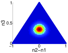
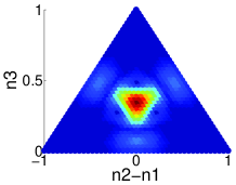
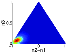
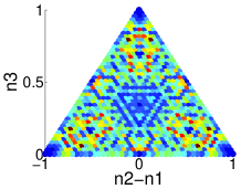
Figure 3: (Color online) Representative eigenstates for the spectrum that is plotted in panel (c) of Fig.​​ 2. Each panel is an image of the probability density in $r$ space, where blue and red correspond to zero and maximum density respectively. (a) The ground-state vortex ${E_{\alpha}\approx-14}$. (b) A metastable vortex ${E_{\alpha}\approx 9}$. (c) A self trapped bright soliton ${E_{\alpha}\approx 62}$. (d) A low purity state in the chaotic sea ${E_{\alpha}\approx 29}$. The color code is blue (low density) to red (high density).

(a)                              (b)                              (c)                              (d)

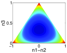
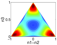
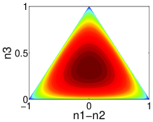
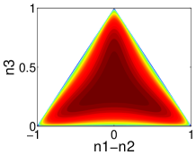
Figure 4: (Color online) Images of the energy surfaces $V_{m}(r)$. Panels (a) and (b) are the bottom ($V_{0}$) and the top ($V_{+}$) energy surfaces for ${(\Phi,u)=(\pi/4,2)}$, illustrating regime (d) in Fig.​​ 6. Panels (c) and (d) are the top energy surfaces for ${(0.8\pi,0.4)}$ and ${(0.8\pi,1.8)}$, illustrating regimes (a) and (b) in Fig.​​ 6. The color code is blue (low energy) to red (high energy). See Fig.​​ 6 for a section along the symmetry line.

VI The energy spectrum

The $E_{\alpha}$ spectrum is plotted in Fig.​​ 2 for several representative parameter sets. Eigenstates are classified by their current ($I$), and color-coded according to their one-particle purity ($S$). In Fig.​​ 3 we display representative examples of eigenstates: the ground-state vortex; a metastable vortex; a self trapped bright soliton; and a low purity microcanonical-like state in the chaotic sea. Inspecting Fig.​​ 2 and Fig.​​ 3, and comparing with the standard picture of Fig.​​ 1, we observe the following:

(A) Mott-Insulator transition: In panels (a)-(d) of Fig.​​ 2 the ground-state is a vortex-state that carries the expected quantized current of Eq.​​ (11). The expected quantized values are indicated in the figures by blue circles. The corresponding ground state wavefuntion is imaged in Fig.​​ 3a. The ground state retains its purity up to an extremely large value of $u$. Beyond a critical value of $u$ the purity of the ground-state is lost. This is evident from the color change of the ground-state from blue in panels 2(a)-2(d) to red in panel 2(e).

(B) Self-trapping: For small $u$, there is a stable vortex-state at the top of the energy landscape, with the expected quantized current of Eq.​​ (11), See e.g. the highest energy current-carrying eigenstate in panel 2(a). If $u$ is large enough, the upper vortex-state bifurcates, and is replaced by 3 self-trapped solitons carrying very little current. See e.g. the self trapped states in panel 2(b), that are represented by 3 overlapping points at the top of the energy landscape, close to the classically expected position marked by the green box. The wavefunction of a self-trapped state is imaged in Fig.​​ 3c.

(C) Metastable vortex states: Looking at panel (c) of Fig.​​ 2 we see that it is feasible to have an additional high purity vortex-state in an intermediate energy range (here around $E\sim 10$). Contrary to the naive expectation, this state has not been mixed with the surrounding continuum, and it caries the expected quantized current of Eq.​​ (11). A representative wavefunction of such state is imaged in Fig.​​ 3b.

(D) Chaotic eigenstates: It should be emphasized, as evident from the continuum of red color points in all panels of Fig.​​ 2, that the majority of eigenstates are highly fragmented and are not characterized by a well-defined quantized value of current. The wavefunction of one such state in imaged in Fig.​​ 3d.

Below we provide a semi-classical interpretation of the above findings, and deduce a schematic diagram of the $(\Phi,u)$ regimes. Self trapping is discussed in Section IX, The Mott transition in Section X, and metastability in Section XI.

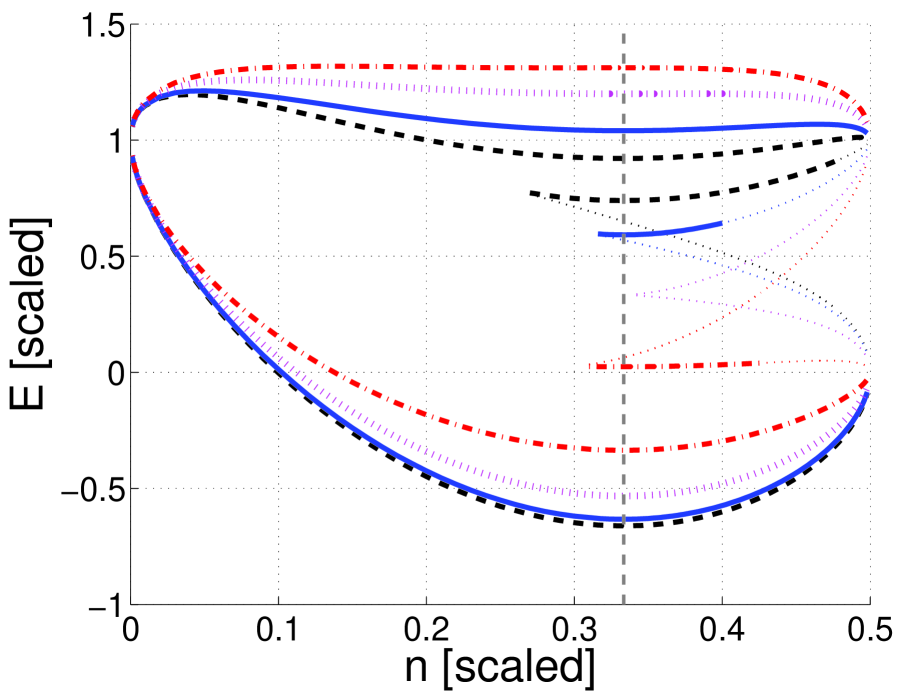
Figure 5: (Color online) A section along the symmetry line ${n_{1}{=}n_{2}{=}n}$, for ${u=2}$ and ${\Phi=\pi/4}$ (solid line), as well as for ${\Phi=0.1\pi}$ (dashed), and $0.5\pi$(dotted), and ${0.8\pi}$ (dashdot). Each section shows the top surface and also the bottom and intermediate surfaces, which are formed of extremal points. The thin dotted segments are formed of saddle points. As $\Phi$ becomes larger the intermediate surface $V_{-}(r)$ goes down in energy. For ${\Phi<\pi/2}$ it is formed of maxima, and its area shrinks to zero as $\Phi$ is increased. For ${\Phi>\pi/2}$ it becomes a surface of minima, and its area expands back.

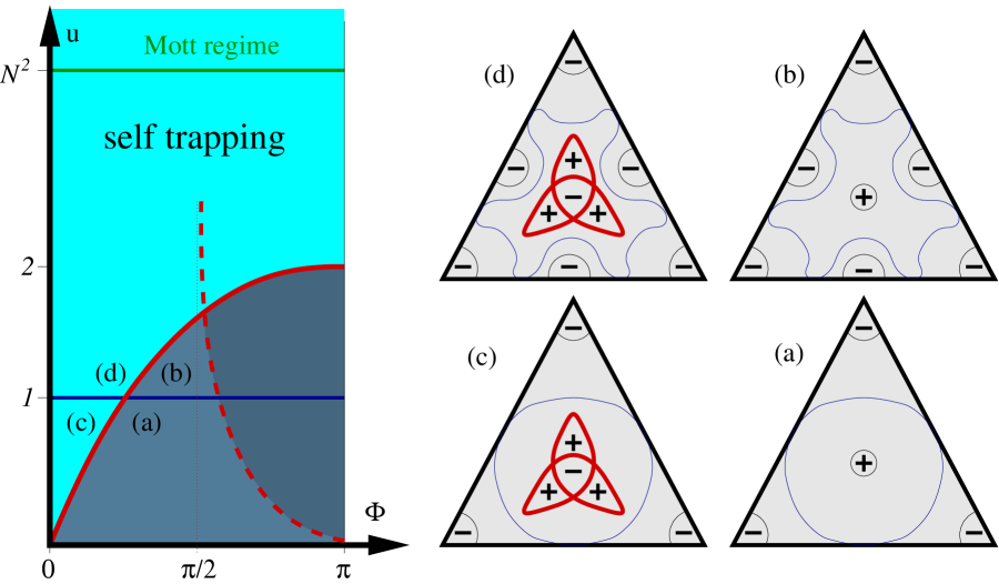
Figure 6: (Color online) Regime diagram of the triangular BEC trimer. The model parameters are $(\Phi,u)$. The thick solid lines divide the diagram into four quarters (a-d). In each quarter the topography of the upper energy surface is different, as schematically illustrated on the right. The thick dashed line indicates the classical stability threshold of the intermediate energy surface. In the quantum analysis we observe quasi-stability as $\Phi=\pi/2$ is crossed: see the text for details and Fig.​​ 8 for demonstration.

VII Stability analysis

The BHH formally describes a set of coupled oscillators. Schematically we can write the Hamiltonian as $H(z)$ with ${z=(r,q)}$ and ${\hbar=1/N}$. This Hamiltonian has $M{-}1$ freedoms. A stable fixed-point $z_{0}$ can support a coherent-state provided $\hbar$ is small enough.

At $r=0$ we always have 3 fixed-points that correspond quantum-mechanically to condensation in one of the 3 momentum orbitals of the trimer. The questions are: (i) whether these fixed-points are stable; (ii) whether they can support a coherent quantum state. In this section we discuss the first question. In Section X (Mott transition) and in Section XI (Metastability) we discuss the second question, which is related to having a finite $\hbar$.

Fixed-point stability is determined by linearization of the Hamiltonian in its vicinity, resulting in a set of Bogolyubov de-Gennes (BdG) equations. This set gives $M{-}1$ frequencies $\omega_{k}$ for the Bogolyubov excitations. Frequencies of different signs imply thermodynamic instability, as occur in Hamiltonian of the type ${H=\omega_{1}n_{1}+\omega_{2}n_{2}}$ with ${\omega_{1}>0}$ and ${\omega_{2}<0}$. Complex frequencies indicate dynamical instability (hyperbolic fixed-point), as occur in Hamiltonian ${H=p^{2}-x^{2}}$. We use here the same terminology as in Udea .

Consider a fixed-point that becomes thermodynamically unstable as a result of varying some parameters in the Hamiltonian, or due to added disorder. This means that the island that had surrounded the fixed-point is now opened. In quantum terms one may say that the former vortex-state can mix with the a finite density of zero-energy excitations, leading to a low purity, possibly ergodic set of eigenstates.

In the remaining part of this section we clarify how the BdG stability analysis is related to the Landau criterion for the stability of a superfluid motion, and mention the known result for an ${M\gg 1}$ ring.

The standard presentation of the Landau criterion takes the liquid as the frame of reference, with the walls moving at some velocity $\Omega$. It is then argued that energy cannot be transferred from the walls to the liquid if the excitation energies satisfy ${\omega_{k}^{(0)}>\Omega k}$ for any wavenumber $k$ of the excitation. In the case of phonons (${\omega_{k}^{(0)}=ck}$) this implies that $\Omega$ should be smaller than the speed of sound $c$.

It is conceptually illuminating to write the Landau criterion in the reference frame where the walls are at rest, and the Hamiltonian becomes time independent. In this frame the superfluid is rotating with frequency ${\Omega_{m}=-\Omega}$. The Landau conditions takes the form ${\omega_{k}>0}$ for any $k$, where

$$\omega_{k}\ \ =\ \ \omega_{k}^{(0)}+\Omega_{m}k,\ \ \ \ \ \ \mbox{[standing device]},$$ (16)

are the excitation energies of the vortex-state. For an $M\gg 1$ ring, taking the continuum limit, the Landau criterion reasoning implies that the excitation energies of the $m$th vortex-state in a rotating device are

$$\omega_{k}\ \ =\ \ \sqrt{\left(\epsilon_{k}+\tilde{u}\right)\epsilon_{k}}\ -\ (\Omega-\Omega_{m})k~{},$$ (17)

where $\Omega=\Phi/(2\pi)$ is the scaled rotation frequency of the device, and $\Omega_{m}=m$ is the quantized rotation frequency of the superfluid. The integer $k$ is the wavenumber of the Bogolyubov excitation, while $\epsilon_{k}=(1/2)k^{2}$ is the unperturbed single-particle energy, and $\tilde{u}$ is the appropriately scaled interaction. The derivation of the first term in Eq.​​ (17) is standard and can be found for example in FV . For small $\epsilon_{k}$ it is common to use a linear approximation $\omega_{k}^{(0)}\approx ck$ where ${c=\sqrt{\tilde{u}/2}}$ is identified as the sound velocity. The second term in Eq.​​ (17) is implied by the Galilean transformation that has been discussed in the previous paragraphs. The implications of Eq.​​ (17) on the stability of the vortex-states is illustrated in Fig.​​ 1.

It should be clear that the Landau criterion is not applicable in the case of a finite $M$ system, because one cannot use a Galilean transformation to relate $\omega_{k}$ to $\omega_{k}^{(0)}$. Therefore we have to utilize the phase-space picture of the dynamics in order to determine the regime diagram of the rotating trimer. Whenever a vortex-state looses its stability, irrespective of the nature of the Bogolyubov excitations, we understand that superfluidity is lost.

The “standing walls” formulation of the Landau-criterion makes transparent the connection to the Fermi-golden-rule picture (FGRP) and to the semi-classical picture (SCP). In the FGRP the vortex-state is perturbed by walls, or optionally by some weak disordered potential. This perturbation induces first-order coupling of the vortex-state to its Bogolyubov one-particle excitations. Accordingly, in the FGRP language the Landau condition is phrased as the requirement of not having Bogolyubov excitations with the same energy as the vortex-state. In the SCP, instead of perturbing the potential, one considers a weak perturbation of the vortex-state. This is like launching several trajectories in the vicinity of the fixed-point, forming an evolving phase-space distribution. The motion is stable if the fixed-point is a local minimum or a local maximum. If the fixed-point is unstable the phase-space distribution deforms and spreads over a large region of the energy shell: consequently the current $I$ is diminished. Technically, this linear-stability analysis leads to the BdG equations discussed in the beginning of this section. As pointed out, the eigenvalues of the BdG equations determine whether the vortex-state is stable or not, leading in the case of translationally-invariant ring to the Landau criterion.

If the vortex-state is meta-stable, then quantum tunnelling or thermal activation are required in order to get a “phase slip” to a lower vortex-state. This goes beyond the “Landau criterion”, but still can be addressed using the SCP, possibly combined with FGRP and optionally using WKB-type approximation.

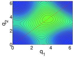
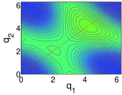
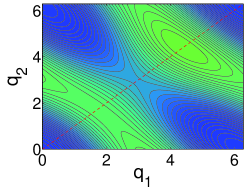
Figure 7: (Color online) Images of $E=\mathcal{H}(r,\varphi)$ as a function of $q_{1}$ and $q_{2}$ for ${\Phi=0.2\pi}$. In the three panels $n_{1}{=}n_{2}{=}n$, hence the fixed-points of interest are along the symmetry line ${q_{1}=q_{2}}$. The left panel is at ${n=(1/10)N}$, and it has a single minimum and a single maximum. The middle panel is at the symmetry point ${r_{0}=0}$, where ${n=(1/3)N}$, and it has a single minimum and two maxima. Consequently in the vicinity of $r_{0}$ we have three energy surfaces. The right panel is at ${n=(9/20)N}$, and it has again a single minimum and a single maximum.

VIII The regimes diagram

We take ${r}$ to be a triangular configuration space. It consists of points ${(\bm{n}_{1},\bm{n}_{2},\bm{n}_{3})}$, such that $\bm{n}_{1}+\bm{n}_{2}+\bm{n}_{3}=N$. The phase differences ${q}$ correspond to the conjugate momenta: they determine the velocity $\dot{r}$. The energy landscape of the Hamiltonian can be visualized using the Peierls-Nabarro surfaces $V_{m}(r)$, formed of its extremal points under phase variation Henn1 ; Henn2 ; Kivshar93 ; Rumpf04 . Lower Peierls-Nabarro surfaces are thus defined as

$$V(r)\ \ \equiv\ \ \min_{\varphi}[\mathcal{H}(r,\varphi)]~{},$$ (18)

whereas upper Peierls-Nabarro surfaces are defined with ${\max[\cdots]}$ instead of ${\min[\cdots]}$. Additionally we may have pieces of surfaces that consists of saddle points.

The Peierls-Nabarro surfaces of the triangular trimer are shown in Fig.​​ 4 (images) and in Fig.​​ 6 (sections). We have 3 Peierls-Nabarro surfaces: (i) a bottom surface $V_{0}(r)$ which is always a “lower surface” (i.e. satisfies Eq. 18), (ii) a top surface $V_{+}(r)$ which is always an “upper surface”, and (iii) an intermediate surface $V_{-}(r)$, which is either an “upper” or a “lower” surface depending on $\Phi$: for ${\Phi<\pi/2}$ it is an “upper” surface that is formed of local maxima, whereas for ${\Phi>\pi/2}$ it is a “lower” surface. The various curves in Fig.​​ 6 illustrate how the intermediate surface $V_{-}(r)$ is modified as a function of the rotation frequency: As $\Phi$ becomes larger this surface goes down in energy, and its area shrinks to zero at ${\Phi=\pi/2}$. As $\Phi$ is increased further its area expands back.

A stable fixed-point is either a minimum of a “lower” surface or a maximum of an “upper” surface. Note also that the upper-most fixed-point can be envisioned as the ground-state of the $U\mapsto-U$ Hamiltonian.

The diagram of Fig.​​ 6 summarizes the different parametric regimes of the model: each regime is characterize by a different type of $V_{m}(r)$ topography. The central point ${r_{0}=0}$ is a fixed-point of the 3 surfaces, with energies $E_{m}=V_{m}(r_{0})$. The fixed point $E_{0}$ is always stable. In contrast, the $E_{\pm}$ fixed-points may be stable or unstable, depending on their curvature $V_{\pm}^{\prime\prime}(r_{0})$, where prime denotes differentiation in the “radial” direction.

The fixed-points are situated on the symmetry lines in $r$ space. So we can restrict the analysis along, say, ${\bm{n}_{1}=\bm{n}_{2}=n}$, hence ${\bm{n}_{3}=N{-}2n}$, and

$$\mathcal{H}(r,q)=\frac{U}{2}\left(\bm{n}_{1}^{2}+\bm{n}_{2}^{2}+\bm{n}_{3}^{2}\right)$$ (19)

$$\ \ \ \ \ \ -K\Big{(}\sqrt{\bm{n}_{2}\bm{n}_{3}}\,\cos\left(q_{1}-\scriptstyle{\frac{\Phi}{3}}\right)+\sqrt{\bm{n}_{3}\bm{n}_{1}}\,\cos\left(q_{2}-\scriptstyle{\frac{\Phi}{3}}\right)$$

$$\ \ \ \ \ \ \ \ \ +\sqrt{\bm{n}_{1}\bm{n}_{2}}\,\cos\left(q_{1}+q_{2}+\scriptstyle{\frac{\Phi}{3}}\right)\Big{)}~{}.$$

The lowest surface ($m=0$) has a trivial topography. In particular for ${\Phi=0}$ the lower surface is

$$V_{0}(r) = \frac{U}{2}\left(\bm{n}_{1}^{2}+\bm{n}_{2}^{2}+\bm{n}_{3}^{2}\right)$$

$$-K\,\left(\sqrt{\bm{n}_{2}\bm{n}_{3}}+\sqrt{\bm{n}_{3}\bm{n}_{1}}+\sqrt{\bm{n}_{1}\bm{n}_{2}}\right)~{}.$$

For general $\Phi$ the extremal values (at a given $r$ location) are still situated along the line $q_{1}=q_{2}$. This is clear by inspection of Eq.​​ (LABEL:e327), which is illustrated in Fig.​​ 7: Depending on $\bm{n}$ and $\Phi$ we have either a single minimum and a single maximum, or two minima and a maximum, or a minimum and two maxima. It follows that one has to find the 3 extremal points $q_{m}(n)$ of the function

$$H(q;n)\ =\ \frac{1}{6}N^{2}U+3U\left(n-\frac{N}{3}\right)^{2}$$ (21)

$$\ \ \ \ -K\left(2\sqrt{(N-2n)n}\,\cos\left(q-\scriptstyle{\frac{\Phi}{3}}\right)+n\,\cos\left(2q+\scriptstyle{\frac{\Phi}{3}}\right)\right)~{}.$$

Then one obtains a section of the surface $V_{m}(r)$ along the principal “radial” direction ${\bm{n}=(n,n,N{-}2n)}$

$$V_{m}(n)\ \ =\ \ H(q_{m}(n);n)~{}.$$ (22)

The most interesting fixed-points of $V_{m}(r)$ are situated at the central point ${\bm{n}=(N/3,N/3,N/3)}$, for which ${n=N/3}$. The three $r_{0}$ fixed-points support the vortex-states. The energies of the fixed-points are:

$$E_{m}=V_{m}(r_{0})=\frac{1}{6}N^{2}U-NK\ \cos\left(\frac{2\pi m-\Phi}{3}\right)\ ~{},$$ (23)

with ${m=0,\pm 1}$. Note consistency with Eq.​​ (10) and the associated expression for the current Eq.​​ (11). A lengthy but straightforward calculation leads to the following result for the curvature at $r_{0}$. This is required in order to determined whether they are stable or not:

$$V_{\pm}^{\prime\prime}(r_{0})\ \ =\ \ \left.\frac{d^{2}H(q_{\pm}(n),n)}{dn^{2}}\right|_{N/3}$$ (24)

$$\ \ =6\frac{K}{N}\left[u-\frac{6-9\cos\left(\frac{\pi\pm 2\Phi}{3}\right)-3\cos\left(\frac{\pi\mp 4\Phi}{3}\right)}{6\cos\left(\frac{\pi\mp\Phi}{3}\right)-2\cos\left(\Phi\right)}\right]~{}.\ \ \ \ \ \$$

We shall use this result in the subsequent discussion of self-trapping and meta-stability.

(a) Current $\langle I\rangle_{+}$                        (b) $1/S_{+}$                                     (c) $1/S_{+}$

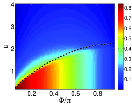
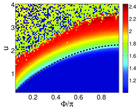
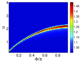
(d) Current $\langle I\rangle_{-}$                        (e) $1/S_{-}$                                     (f) correlation

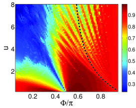
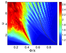
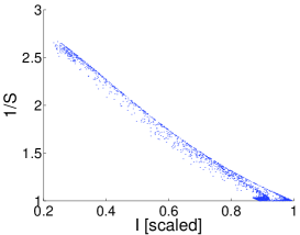
Figure 8: (Color online) We consider a trimer with $N=42$ bososns. In (a) The current of the upper-energy state is imaged as a function of $(\Phi,u)$. It becomes vanishingly small once the self-trapping border (dashed line) is crossed. In (b) we plot the $1/S$ of the same state, while in (c) we repeat the calculation after adding some weak disorder $\epsilon{\sim}0.01$ (see text). Panels (d) and (e) are the same as (a) and (b) but for the intermediate state that has the maximal current. This is a metastable vortex-state if ${S\sim 1}$. Note that the classical stability border (dashed line) fails to provide a valid prediction for loss of purity, which is strongly correlated with low $I$ values as demonstrated in panel (f).

IX Self trapping

Let us first recall the well-known phase-space analysis of the $M{=}2$ dimer. A concise detailed account can be found in Section II of csd . For ${u<1}$ the energy landscape stretches between a minimum that corresponds to condensation in the lower orbital, and a maximum that corresponds to condensation in the upper orbital. For ${u>1}$ the maximum bifurcates and accordingly there are two elliptic islands of self-trapped motion. See Fig.1 of csd for illustration.

Going back to the trimer, one realizes that the dimer type bifurcation at ${u=1}$ takes place along the edges of the upper energy surface $V_{+}(r)$. This bifurcation is schematically illustrated in going from Fig.​​ 6ac to Fig.​​ 6bd. Namely, for ${u>1}$ there are two maxima along each edge. But these maxima are merely the corners of the central region. The maximum energy is located higher: either in the center (Fig.​​ 6b) or bifurcated into three fixed-points (Fig.​​ 6d). Hence ${u=1}$ is not the threshold for self-trapping.

Self-trapping in the trimer is related to the stability of the $r_{0}$ fixed-point in the upper energy surface. If ${V_{+}^{\prime\prime}(r_{0})>0}$ this upper vortex-state bifurcates into 3 maxima that support “self-trapped” states, also known as bright solitons. This bifurcation is schematically illustrated in going from Fig.​​ 6ab to Fig.​​ 6cd. The self-trapping transition is reflected in the current dependence as demonstrated in Fig.​​ 8. Namely, the current in panel (a) becomes very small once the classical stability border (dashed curve) is crossed. In panel (b) we confirm that the loss of stability is reflected by loss of purity: once the $r_{0}$ fixed-point looses stability the vortex-state is replaced by 3 soliton-band-states that stretch over the 3 fixed-point.

In Fig.​​ 8c we repeat the calculation as in Fig.​​ 8b, but with added weak disorder. Namely, we add small on-site energy-shifts $\epsilon_{j}a_{j}^{{\dagger}}a_{j}$ to the Hamiltonian Eq.​​ (5) in order to break the translational invariance of the system. These added random shifts are much smaller than the inter-site hopping $K$. They do not affect the stability of the vortex states but they prevent the formation of a soliton band. Note that for ${M\gg 1}$ the soliton band would be exponentially narrow. Due to the added weak diorder the soliton-band states disintegrate into self-trapped coherent states that have high purity. In fact some self-trapping also happens in the numerics of panel (b) due to the finite accuracy of the computer. The same numerical issue is well known with regard to self-trapping in the dimer system nst1 ; nst2 .

The above bifurcation scenario appears contradictory to common wisdom. For an $M$ site ring self-trapping is anticipated when the self-induced potential is deeper than the binding energy, leading to the condition ${u^{cl}>1}$, where

$${u^{cl}\ \ =\ \ \frac{2}{M}u~{}.}$$ (25)

Contrary to this naive expectation, Eq.​​ (LABEL:e6) for the trimer implies that the threshold for self-localization is vanishingly small at the limit ${\Phi\rightarrow 0}$. The explanation for this anomaly is as follows: for $\Phi=0$ the ${m=\pm 1}$ angular-momentum orbitals are degenerate, hence any small $U$ results in 3 maxima in $V_{+}(r)$. In the case of an $M$ site ring any small $U$ results in $M$ maxima. But if $M\gg 1$ these maxima represent states that have very weak modulation in the site occupation rather than self-trapping.

X Mott transition

The BEC ground-state corresponds to the minimum of the lower $V(r)$ surface, which is an elliptic island. If $u$ is too large this island becomes too small to support a coherent-state and the ground-state number-squeezes towards a Fock-basis state. For a Bose-Hubbard dimer ($M{=}2$) the ground-state becomes a fragmented Fock-state of ${50\%-50\%}$ site occupation if ${u>N^{2}}$. See e.g. csd . More generally, for an $M$ site ring, the Mott superfluid-insulator transition is controlled by the quantum dimensionless parameter

$${u^{qm}\ \ =\ \ \frac{Mu}{N^{2}}~{}.}$$ (26)

As $u^{qm}>1$ the ground-state looses its one-body coherence and approaches a Fock-state of equal site occupation.

The regimes of Fig.​​ 6 that are implied by the “classical” stability analysis, are related to the topology of phase-space: they can be resolved if $\hbar$ is reasonably small, but do not depend on $\hbar$. (Note again that $\hbar=1/N$ reflects the total number of particle in the system). In contrast, the “quantum” Mott transition has to do with having a finite $\hbar$. As $u$ is increased the area of the lower stability island becomes smaller. Due to having a finite Planck-cell, the shrinking lower surface of the Hamiltonian cannot support a coherent-state if $u$ becomes too large. Instead there appear a glassy set of low energy fragmented Fock-states. The transition is observed in Fig.​​ 2. Namely, as implied by the term “glassiness”, one observes in panel (e) a non-zero density of low energy states, as opposed to panels (a-d) of the same figure where the ground state is situated in a well defined location. The observed glassiness is due to the possibility to play with the occupation whenever $N/M$ is not an integer, or due to having some on-site disorder. The Mott transition becomes “sharp” only in the thermodynamic limit of having large $M$, keeping $N/M$ constant.

XI Metastability

Having examined the minimum of the lowest Peierls-Nabarro surface $V_{0}(r)$ that undergoes a Mott transition, and the maximum of upper surface $V_{+}(r)$ in connection with self-trapping, we turn our attention to the intermediate surface $V_{-}(r)$. We observe in Fig.​​ 2 that a dynamically (meta)stable vortex-states can be found in the middle of the energy spectrum. The $\Phi$ threshold for stabilization is deduced from the condition ${V_{-}^{\prime\prime}(r_{0})>0}$ provided $V_{-}(r)$ is a “lower” surface. This border is illustrated schematically in Fig.​​ 6 and analytically in Fig.​​ 8 (dashed black line). Unlike self-trapping, here this (classical) border is barely reflected in the numerical results. One observes that large current that is supported by high purity vortex-state appear well beyond the expected stability region. Thus a coherent-solution can be quantum-mechanically stabilized in a flat landscape by interference. We refer to this as “quasi-stability”.

What we call quasi-stability is the possibility to have a quantum coherent eigenstate that is supported by an unstable fixed-point. If we have an hyperbolic fixed-point that is immersed in a chaotic sea this is known as “quantum scarring” scars1 ; scars2 . Another well known example for quasi-stability is the Anderson strong-localization effect AL .

Let us point out two examples for quasi-stability in the BHH context. The simplest example is apparently the condensation of bosons in the upper orbital of a dimer csf : this is formally the same as saying that the upper position of a pendulum is quasi-stable rather than unstable. An additional example is encountered in the case of a kicked dimer ckt , which is a manifestation of quantum scarring scars1 ; scars2 . In both examples the quasi-stability is related to the low participation number (PN). The PN characterizes a coherent-state that is situated on the hyperbolic point; it estimates how many eigenstates appear in its spectral decomposition. In the first example the deterioration of the purity is small because PN$\,\sim\log(N)$ rather than PN$\,\sim\sqrt{N}$, while in the second example PN$\,\sim N$ with a prefactor that depends on the Lyapunov exponent.

It seems to us that in the present analysis the traditional paradigms for quantum quasi-stability do not apply. The natural tendency is to associate the observed quasi-stability with quantum scarring, and to proceed with the analysis as in ckt . If this were the case, quasi-stability would be related to the curvature at $r_{0}$. This curvature becomes worse as we cross $\Phi=\pi/2$. But the patterns in Fig.​​ 8 are not correlated with $V^{\prime\prime}(r_{0})$. We thus conclude that a new paradigm is required.

XII Concluding remarks

We presented a comprehensive overview of a minimal model for a superfluid circuit. Contrary to the conventional picture we observe that self-trapping can occur for arbitrarily small interaction, and that unstable vortex-states can become quasi-stable. These anomalies reflect the mesoscopic nature of the device: effects that are related to orbital-degeneracy and quantum-scarring cannot be neglected.

A two orbital approximation as in Brand2 does not qualify as a minimal model for a superfluid circuit, but it captures one essential ingredient: as a parameter is varied a fixed-point can undergo a bifurcation. Specifically a vortex-state can bifurcate into solitons. In the absence of symmetry breaking the bifurcation is into $M$ solitons, as illustrated in Fig.​​ 2 in going from regime (a) to regime (c). These solitons form a band unless the displacement symmetry is broken, say by disorder. The 2 orbital approximation assumes such symmetry breaking, and provides a simplified local description of the bifurcation. A global description of phase-space topology requires to go beyond the 2 orbital approximation. Then one encounters eigenstates that dwell in the chaotic sea. Consequently one can regard the trimer as a bridge towards the classical and the thermodynamic limits. All the required ingredients are here: the topology and the underlying mixed phase-space.

We note that in a former work Ghosh it has been argued that for $\Omega=0$ metastable vortex-states would be found provided ${M>4}$. The argument explicitly assumes ${\Omega=0}$, and it is based on a semiclassical (mean field) stability analysis. We find that for ${\Omega\neq 0}$ the semiclassical stability analysis allows metastable vortex-states for ${M=3}$ as well. The results of our semiclassical analysis are summarized by the ${(\Omega,u)}$ regime diagram of Fig.​​ 6.

But when we go to the quantum analysis we find that the physical picture is further modified quite dramatically due to the manifestation of quantum interference effect that is not expected on the basis of a mean-field theory. This unexpected quasi-stability is effective enough to stabilize metastable vortex-states even if the device is non-rotating!

Note added in proof.– Relevant works have been brought to our attention recently P1 ; P2 ; P3 .

Acknowledgments.– We thank James Anglin, Tony Leggett, and Parag Ghosh for useful communication regrading the observation that for $\Omega=0$ metastable vortex-states would be found provided ${M>4}$. We thank Igor Tikhonenkov and Christine Khripkov for sharing numerical codes that had been used in trm . This research was supported by the Israel Science Foundation (grant Nos. 29/11 and 346/11) and by the US-Israel Binational Science Foundation (grant No. 2008141).

References

- (1) C. Raman, M. Kohl, R. Onofrio, D.S. Durfee, C.E. Kuklewicz, Z. Hadzibabic, W. Ketterle, Phys. Rev. Lett. 83, 2502 (1999).
- (2) R. Onofrio, C. Raman, J.M. Vogels, J.R. Abo-Shaeer, A.P. Chikkatur, W. Ketterle, Phys. Rev. Lett. 85, 2228 (2000).
- (3) S. Inouye, S. Gupta, T. Rosenband, A.P. Chikkatur, A. Gorlitz, T.L. Gustavson, A.E. Leanhardt, D.E. Pritchard, W. Ketterle, Phys. Rev. Lett. 87, 080402 (2001).
- (4) M. Albiez, R. Gati, J. Folling, S. Hunsmann, M. Cristiani, M.K. Oberthaler, Phys. Rev. Lett. 95, 010402 (2005).
- (5) P. Engels, C. Atherton, Phys. Rev. Lett. 99, 160405 (2007).
- (6) D.E. Miller, J.K. Chin, C.A. Stan, Y. Liu, W. Setiawan, C. Sanner, W. Ketterle, Phys. Rev. Lett. 99, 070402 (2007).
- (7) S. Levy, E. Lahoud, I. Shomroni, J. Steinhauer, Nature (London) 449, 579 (2007).
- (8) C. Ryu, M.F. Andersen, P. Clade, V. Natarajan, K. Helmerson, W.D. Phillips, Phys. Rev. Lett. 99, 260401 (2007).
- (9) D. McKay, M. White, M. Pasienski, B. DeMarco, Nature 453, 76 (2008).
- (10) T.W. Neely, E.C. Samson, A.S. Bradley, M.J. Davis, B.P. Anderson, Phys. Rev. Lett. 104, 160401 (2010).
- (11) L.J. LeBlanc, A.B. Bardon, J. McKeever, M.H.T. Extavour, D. Jervis, J.H. Thywissen, F. Piazza, A. Smerzi, Phys. Rev. Lett. 106, 025302 (2011).
- (12) R. Desbuquois, L. Chomaz, T. Yefsah, J. Leonard, J. Beugnon, C. Weitenberg, and J. Dalibard, Nat. Phys. 8, 645 (2012).
- (13) S. Moulder, S. Beattie, R. P. Smith, N. Tammuz, Z. Hadzibabic, Phys. Rev. A 86, 013629 (2012).
- (14) A. Ramanathan, K.C. Wright, S. R.Muniz, M. Zelan, W.T. Hill, C.J. Lobb, K. Helmerson, W.D. Phillips, G.K. Campbell, Phys. Rev. Lett. 106, 130401 (2011).
- (15) K.C. Wright, R.B. Blakestad, C.J. Lobb, W.D. Phillips, G.K. Campbell, Phys. Rev. Lett. 110, 025302 (2013)
- (16) M. Cominotti, D. Rossini, M. Rizzi, F. Hekking, A. Minguzzi, arXiv:1310.0382
- (17) R. Kanamoto, H. Saito, M. Ueda, Phys. Rev. A 68, 043619 (2003),
- (18) R. Kanamoto, L.D. Carr, M. Ueda, Phys. Rev. Lett. 100, 060401 (2008)
- (19) R. Kanamoto, L.D. Carr, M. Ueda, Phys. Rev. A 79, 063616 (2009)
- (20) A.Yu. Cherny, J.-S. Caux, J. Brand, Frontiers of Physics 7, 54 (2012)
- (21) R. Ozeri, N. Katz, J. Steinhauer, N. Davidson, Rev. of Mod. Phys. 77, 187 (2005).
- (22) L.D. Landau, J. Phys. (Moscow) 5, 71 (1941).
- (23) V, Hakim, Phys. Rev. E 55, 2835–2845 (1997)
- (24) M. Albert, T. Paul, N. Pavloff, P. Leboeuf, Phys. Rev. A 82, 011602(R) (2010)
- (25) O. Morsch, M. Oberthaler, Rev. Mod. Phys. 78, 179 (2006).
- (26) I. Bloch, J. Dalibard, and W. Zwerger, Rev. Mod. Phys. 80, 885 (2008).
- (27) I. Brezinova, A.U.J. Lode, A.I. Streltsov, O.E. Alon, L.S. Cederbaum, J. Burgdorfer, Phys. Rev. A 86, 013630 (2012)
- (28) A.I. Streltsov, K. Sakmann, O.E. Alon, L.S. Cederbaum, Phys. Rev. A 83, 043604 (2011)
- (29) A. Polkovnikov, E. Altman, E. Demler, B. Halperin, M.D. Lukin, Phys. Rev. A 71, 063613 (2005)
- (30) O. Fialko, M.-C. Delattre, J. Brand, A.R. Kolovsky, Phys. Rev. Lett. 108, 250402 (2012)
- (31) J. C. Eilbeck, G. P. Tsironis, and S. K. Turitsyn, Phys. Scr. 52, 386 (1995).
- (32) D. Hennig, H. Gabriel, M.F. Jorgensen, P.L. Christiansen, and C.B. Clausen, Phys. Rev. E 51, 2870 (1995).
- (33) S. Flach and V. Fleurov, J. Phys.: Condens. Matter 9, 7039 (1997).
- (34) K. Nemoto, C.A. Holmes, G.J. Milburn, and W.J. Munro, Phys. Rev. A 63, 013604 (2000).
- (35) R. Franzosi, V. Penna, Phys. Rev. A 65, 013601 (2002).
- (36) R. Franzosi, V. Penna, Phys. Rev. E 67, 046227 (2003).
- (37) M. Hiller, T. Kottos, and T. Geisel, Phys. Rev. A 73, 061604(R) (2006).
- (38) E. M. Graefe, H. J. Korsch, and D. Witthaut, Phys. Rev. A 73, 013617 (2006).
- (39) J. D. Bodyfelt, M. Hiller, and T. Kottos, Europhys. Lett. 78, 50003 (2007).
- (40) P. Buonsante, V. Penna, J. Phys. A 41, 175301 (2008)
- (41) M. Hiller, T. Kottos, and T. Geisel, Phys. Rev. A 79, 023621 (2009).
- (42) T.F. Viscondi, K. Furuya, J. Phys. A 44, 175301 (2011)
- (43) P. Jason, M. Johansson, K. Kirr, Phys. Rev. E 86, 016214 (2012)
- (44) H. Hennig, J. Dorignac, D.K. Campbell, Phys. Rev. A 82, 053604 (2010) l
- (45) Holger Hennig, Ragnar Fleischmann, Phys. Rev. A 87, 033605 (2013)
- (46) T. Kottos, B. Shapiro, Phys. Rev. E 83, 062103 (2011)
- (47) I. Tikhonenkov, A. Vardi, J.R. Anglin, D. Cohen, Phys. Rev. Lett. 110, 050401 (2013).
- (48) Y.S. Kivshar and D. K. Campbell, Phys. Rev. E 48, 3077 (1993).
- (49) B. Rumpf, Phys. Rev. E 70, 016609 (2004).
- (50) A.M. Perelomov, Commun. Math. Phys. 26, 222 (1972); arXiv:math-ph/0203002
- (51) Quantum Theory of Many-Particle Systems A.L. Fetter, J.D. Walecka, (McGraw-Hill 1971, Dover Books 2003)
- (52) M. Chuchem, K. Smith-Mannschott, M. Hiller, T. Kottos, A. Vardi, D. Cohen, Phys. Rev. A 82, 053617 (2010).
- (53) Y.P. Huang, M.G. Moore, Phys. Rev. A 73, 023606 (2006).
- (54) D.R. Dounas-Frazer, A.M. Hermundstad, L.D. Carr, Phys. Rev. Lett. 99, 200402 (2007)
- (55) E.J. Heller, in Chaos and Quantum Physics, edited by A. Voros and M.-J. Giannoni, Proceedings of the Les-Houches Summer School of Theoretical Physics, Session LII (North-Holland, Amsterdam, 1990).
- (56) L. Kaplan, E.J. Heller, Phys. Rev. E 59, 6609 (1999).
- (57) B. Kramer, A. MacKinnon, Rep. Prog. Phys. 56, 1469 (1993).
- (58) C. Khripkov, D. Cohen, A. Vardi, J. Phys. A 46, 165304 (2013).
- (59) C. Khripkov, D. Cohen, A. Vardi, Phys. Rev. E 87, 012910 (2013).
- (60) P. Ghosh, F. Sols, Phys. Rev. A 77, 033609 (2008)
- (61) P. Buonsante, V. Penna, A. Vezzani, Phys. Rev. A 82, 043615 (2010).
- (62) P. Buonsante, V. Penna, A. Vezzani, Phys. Rev. A 84, 061601 (2011).
- (63) P. Buonsante, L. Orefice, A. Smerzi, Phys. Rev. A 87, 063620 (2013).