A Domain Decomposition Approach to Implementing Fault Slip in Finite-Element Models of Quasi-static and Dynamic Crustal Deformation

Abstract

We employ a domain decomposition approach with Lagrange multipliers to implement fault slip in a finite-element code, PyLith, for use in both quasi-static and dynamic crustal deformation applications. This integrated approach to solving both quasi-static and dynamic simulations leverages common finite-element data structures and implementations of various boundary conditions, discretization schemes, and bulk and fault rheologies. We have developed a custom preconditioner for the Lagrange multiplier portion of the system of equations that provides excellent scalability with problem size compared to conventional additive Schwarz methods. We demonstrate application of this approach using benchmarks for both quasi-static viscoelastic deformation and dynamic spontaneous rupture propagation that verify the numerical implementation in PyLith.

AAGAARD ET AL. FAULT SLIP VIA DOMAIN DECOMPOSITION B. T. Aagaard, USGS MS977, 345 Middlefield Rd, Menlo Park, CA 94025, USA. (baagaard@usgs.gov) M. G. Knepley, Computation Institute, University of Chicago, Searle Chemistry Laboratory, 5735 S. Ellis Avenue, Chicago, IL 60637, USA. C. A. Williams, GNS Science, 1 Fairway Drive, Avalon, PO Box 30368, Lower Hutt 5040, New Zealand.

This information is distributed solely for the purpose of predissemination peer review and must not be disclosed, released, or published until after approval by the U.S. Geological Survey (USGS). It is deliberative and predecisional information and the findings and conclusions in the document have not been formally approved for release by the USGS. It does not represent and should not be construed to represent any USGS determination or policy.

1 Introduction

The earthquake cycle, from slow deformation associated with interseismic behavior to rapid deformation associated with earthquake rupture, spans spatial scales ranging from fractions of a meter associated with the size of contact asperities on faults and individual grains to thousands of kilometers associated with plate boundaries. Similarly, temporal scales range from fractions of a second associated with slip at a point during earthquake rupture to thousands of years of strain accumulation between earthquakes. The complexity of the many physical processes operating over this vast range of scales leads most researchers to focus on a narrow space-time window to isolate just one or a few processes; the limited spatial and temporal coverage of observations also often justifies this narrow focus.

Researchers have recognized for some time, though, that interseismic deformation and fault interactions influence earthquake rupture propagation, and the dynamics of rupture propagation, in turn, affect postseismic deformation (Igarashi et al., 2003; Ito et al., 2007; Chen and Lapusta, 2009; Matsuzawa et al., 2010). In most cases one simplifies some portion of the process to expedite the modeling results of another portion. For example, studies of slow deformation associated with interseismic and postseismic behavior often approximate dynamic rupture behavior with the static coseismic slip (Reilinger et al., 2000; Pollitz et al., 2001; Langbein et al., 2006; Chlieh et al., 2007). Likewise, studies of rapid deformation associated with earthquake rupture propagation often approximate the loading of the crust at the beginning of a rupture (Mikumo et al., 1998; Harris and Day, 1999; Aagaard et al., 2001; Peyrat et al., 2001; Oglesby and Day, 2001; Dunham and Archuleta, 2004). Numerical seismicity models that attempt to model multiple earthquake cycles generally simplify not only the fault loading and rupture propagation, but also the physical properties to make the calculations tractable (Ward, 1992; Robinson and Benites, 1995; Hillers et al., 2006; Rundle et al., 2006; Pollitz and Schwartz, 2008; Dieterich and Richards-Dinger, 2010).

Some dynamic spontaneous rupture modeling studies have attempted to examine a broader space-time window to remove simplifying assumptions and more accurately capture the complex interactions over the earthquake cycle. For example, Duan and Oglesby (2005) simulated multiple earthquake cycles on a fault with a bend to capture the spatial variation in the stress field around the bend, which they found to have a strong role in determining whether a rupture would propagate past the bend. By spinning up the model over many earthquake cycles, they obtained a much more realistic stress field immediately prior to rupture compared with assuming a simple stress field or calculating the stress field from a static analysis. Chen and Lapusta (2009) examined the behavior of small repeating earthquakes by modeling a stable sliding region (friction increases with slip rate) surrounding an unstable sliding region (friction decreases with slip rate). They found that the aseismic slip occurring within the unstable patch between ruptures contributed a significant fraction of the long-term slip. As a result, their simulations displayed a complex interaction between aseismic slip between earthquakes and coseismic slip that would not have been possible if they did not explicitly model the interseismic deformation.

Kaneko et al. (2011) developed more sophisticated earthquake cycle models using spectral element simulations that permit spatial variations in physical properties that capture the dynamic rupture propagation as well as the interseismic deformation. They examined the effects of low-rigidity layers and a fault damaged zone on rupture dynamics. In addition to purely dynamic effects, such as amplified slip rates during dynamic rupture, they found several effects that required resolving both the interseismic deformation and the rapid slip during dynamic rupture; the low-rigidity layers reduced the nucleation size, amplified slip rates during dynamic rupture, increased the recurrence interval, and reduced the amount of aseismic slip.

Reproducing observed earthquake cycle behavior remains a challenge. Barbot et al. (2012) applied boundary integral simulation techniques to develop an earthquake cycle model of Mw 6.0 Parkfield, California, earthquakes. They employed spatial variation of the fault constitutive properties for Dieterich-Ruina rate-state friction to yield regions with stable sliding and regions with stick-slip behavior. This allowed their numerical model to closely match the observed geodetic interseismic behavior as well as the slip pattern of the 2004 Parkfield earthquake. Nevertheless, some aspects of the physical process, such as the 3-D nonplanar flower-structure geometry of the San Andreas fault and 3-D variation in elastic properties were not included in the Barbot et al. (2012) model.

Collectively, these studies suggest a set of desirable features for models of the earthquake cycle to capture both the slow deformation associated with interseismic behavior and the rapid deformation associated with earthquake rupture propagation. These features include the general capabilities of modeling elasticity with elastic, viscoelastic, and viscoelastoplastic rheologies, as well as slip on faults via either prescribed ruptures or spontaneous ruptures controlled by a fault constitutive model. Additionally, a model could also include the coupling of elasticity to fluid and/or heat flow.

With the goal of modeling the entire earthquake cycle with as few simplifications as possible, much of our work in developing PyLith has focused on modeling fault slip with application to quasi-static simulations of interseismic and coseismic deformation and dynamic simulations of earthquake rupture propagation. This effort builds on our previous work on developing the numerical modeling software EqSim (Aagaard et al., 2001) for dynamic spontaneous rupture simulations and Tecton (Melosh and Raefsky, 1980; Williams and Richardson, 1991) for quasi-static interseismic and postseismic simulations. We plan to seamlessly couple these two types of simulations together to resolve the earthquake cycle. Implementing slip on the potentially nonplanar fault surface differentiates these types of problems from many other elasticity problems. Complexities arise because earthquakes may involve offset on multiple, intersecting irregularly shaped fault surfaces in the interior of a modeling domain. Furthermore, we want the flexibility to either prescribe the slip on the fault or have the fault slip evolve according to a fault constitutive model that specifies the friction on the fault surface. Here, we describe a robust, yet flexible method for implementing fault slip with a domain decomposition approach, its effect on the overall design of PyLith, and verification of its implementation using benchmarks.

2 Numerical Model of Fault Slip

In this section we summarize the formulation of the governing equations using the finite-element method. We augment the conventional finite-element formulation for elasticity with a domain decomposition approach (Smith et al., 1996; Zienkiewicz et al., 2005) to implement the fault slip. The PyLith manual (Aagaard et al., 2012) provides a step-by-step description of the formulation.

We solve the elasticity equation including inertial terms,

$$\rho\frac{\partial^{2}\bm{u}}{\partial t^{2}}-\bm{f}-\boldsymbol{\nabla}\cdot\bm{\sigma}=\bm{0}\text{ in }V,$$ (1)

$$\bm{\sigma}\cdot\bm{n}=\bm{T}\text{ on }S_{T},$$ (2)

$$\bm{u}=\bm{u}_{0}\text{ on }S_{u},$$ (3)

$$\bm{d}-(\bm{u}_{+}-\bm{u}_{-})=\bm{0}\text{ on }S_{f},$$ (4)

where $\bm{u}$ is the displacement vector, $\rho$ is the mass density, $\bm{f}$ is the body force vector, $\bm{\sigma}$ is the Cauchy stress tensor, and $t$ is time. We specify tractions $\bm{T}$ on surface $S_{T}$, displacements $\bm{u_{0}}$ on surface $S_{u}$, and slip $\bm{d}$ on fault surface $S_{f}$, where the tractions and fault slip are in global coordinates. Because both $\bm{T}$ and $\bm{u}$ are vector quantities, there can be some spatial overlap of the surfaces $S_{T}$ and $S_{u}$; however, a degree of freedom at any location cannot be associated with both prescribed displacements (Dirichlet) and traction (Neumann) boundary conditions simultaneously.

Following a conventional finite-element formulation (ignoring the fault surface for a moment), we construct the weak form by taking the dot product of the governing equation with a weighting function and setting the integral over the domain equal to zero,

$$\int_{V}\boldsymbol{\phi}\cdot\left(\boldsymbol{\nabla}\cdot\bm{\sigma}+\bm{f}-\rho\frac{\partial^{2}\bm{u}}{\partial t^{2}}\right)\,dV=0.$$ (5)

The weighting function $\boldsymbol{\phi}$ is a piecewise differentiable vector field with $\boldsymbol{\phi}=\bm{0}$ on $S_{u}$. After some algebra and use of the boundary conditions (equations (2) and (3)), we have

$$\begin{split}-\int_{V}\nabla\boldsymbol{\phi}:\bm{\sigma}\,dV+\int_{S_{T}}\boldsymbol{\phi}\cdot\bm{T}\,dS+\int_{V}\boldsymbol{\phi}\cdot\bm{f}\,dV\\ -\int_{V}\boldsymbol{\phi}\cdot\rho\frac{\partial^{2}\bm{u}}{\partial t^{2}}\,dV=0,\end{split}$$ (6)

where $\nabla\boldsymbol{\phi}:\bm{\sigma}$ is the double inner product of the gradient of the weighting function and the stress tensor.

Using a domain decomposition approach, we consider the fault surface as an interior boundary between two domains as shown in Figure 1. We assign a fault normal direction to this interior boundary and “positive” and “negative” labels to the two sides of the fault, such that the fault normal is the vector from the negative side of the fault to the positive side of the fault. Slip on the fault is the displacement of the positive side relative to the negative side. Slip on the fault also corresponds to equal and opposite tractions on the positive ($\bm{l_{+}}$) and negative ($\bm{l_{-}}$) sides of the fault, which we impose using Lagrange multipliers with $\bm{l}_{+}+\bm{l}_{-}=0$.

Recognizing that the tractions on the fault surface are analogous to the boundary tractions, we add in the contributions from integrating the Lagrange multipliers (fault tractions) over the fault surface,

$$\begin{split}-\int_{V}\nabla\boldsymbol{\phi}:\bm{\sigma}\,dV+\int_{S_{T}}\boldsymbol{\phi}\cdot\bm{T}\,dS-\int_{S_{f^{+}}}\boldsymbol{\phi}\cdot\bm{l}\,dS\\ +\int_{S_{f^{-}}}\boldsymbol{\phi}\cdot\bm{l}\,dS+\int_{V}\boldsymbol{\phi}\cdot\bm{f}\,dV-\int_{V}\boldsymbol{\phi}\cdot\rho\frac{\partial^{2}\bm{u}}{\partial t^{2}}\,dV=0.\end{split}$$ (7)

Our sign convention for the fault normal and fault tractions (tension is positive) leads to the Lagrange multiplier terms having the opposite sign as the boundary tractions term. We also construct the weak form for the constraint associated with slip on the fault by taking the dot product of the constraint equation with the weighting function and setting the integral over the fault surface to zero,

$$\int_{S_{f}}\boldsymbol{\phi}\cdot\left(\bm{d}-\bm{u}_{+}+\bm{u}_{-}\right)\,dS=0.$$ (8)

This constraint equation applies to the relative displacement vector across the fault and slip in the tangential and fault opening directions.

The domain decomposition approach for imposing fault slip or tractions on a fault is similar to the “split nodes” and “traction at split nodes” (TSN) techniques used in a number of finite-difference and finite-element codes (Melosh and Raefsky, 1981; Andrews, 1999; Bizzarri and Cocco, 2005; Day et al., 2005; Duan and Oglesby, 2005; Dalguer and Day, 2007; Moczo et al., 2007), but differs from imposing fault slip via double couple point sources. The domain decomposition approach treats the fault surface as a frictional contact interface, and the tractions correspond directly to the Lagrange multipliers needed to satisfy the constraint equation involving the jump in the displacement field across the fault and the fault slip. As a result, the fault tractions are equal and opposite on the two sides of the fault and satisfy equilibrium. The TSN technique is often applied in dynamic spontaneous rupture models with explicit time stepping and a diagonal system Jacobian, so that the fault tractions are explicitly computed as part of the solution of the uncoupled equations. In this way the TSN technique as described by Andrews (1999) could be considered an optimization of the domain decomposition technique for the special case of dynamic spontaneous rupture with a fault constitutive model and explicit time stepping.

Imposing fault slip via double couple point sources involves imposing body forces consistent with an effective plastic strain associated with fault slip (sometimes called the “stress-free strain” (Aki and Richards, 2002)). The total strain is the superposition of this effective plastic strain and the elastic strain. The fault tractions are associated with the elastic strain. This illustrates a key difference between this approach and the domain decomposition approach in which the Lagrange multipliers and the constraint equation directly relate the fault slip to the fault tractions (Lagrange multipliers). One implication of this difference is that when using double couple point forces, the body forces driving slip depend on the elastic modulii and will differ across a fault surface with a contrast in the elastic modulii, whereas the fault tractions (Lagrange multipliers) in the domain decomposition approach will be equal in magnitude across the fault.

We express the weighting function $\boldsymbol{\phi}$, trial solution $\bm{u}$, Lagrange multipliers $\bm{l}$, and fault slip $\bm{d}$ as linear combinations of basis functions,

$$\boldsymbol{\phi}=\sum_{m}\bm{a}_{m}N_{m},$$ (9)

$$\bm{u}=\sum_{n}\bm{u}_{n}N_{n},$$ (10)

$$\bm{l}=\sum_{p}\bm{l}_{p}N_{p},$$ (11)

$$\bm{d}=\sum_{p}\bm{d}_{p}N_{p}.$$ (12)

Because the weighting function is zero on $S_{u}$, the number of basis functions for the trial solution $\bm{u}$ is generally greater than the number of basis functions for the weighting function $\boldsymbol{\phi}$, i.e., $n>m$. The basis functions for the Lagrange multipliers and fault slip are associated with the fault surface, which is a lower dimension than the domain, so $p\ll n$ in most cases. If we express the linear combination of basis functions in terms of a matrix-vector product, we have

$$\boldsymbol{\phi}=\bm{N}_{m}\cdot\bm{a}_{m},$$ (13)

$$\bm{u}=\bm{N}_{n}\cdot\bm{u}_{n},$$ (14)

$$\bm{l}=\bm{N}_{p}\cdot\bm{l}_{p},$$ (15)

$$\bm{d}=\bm{N}_{p}\cdot\bm{d}_{p}.$$ (16)

The first term on the right hand side of these equations is a matrix of the basis functions. For example, in three dimensions $\bm{N}_{m}$ is a $3\times 3m$ matrix, where $m$ is the number of basis functions.

The weighting function is arbitrary, so the integrands must be zero for all $\bm{a}_{m}$, which leads to

$$\begin{split}-\int_{V}\nabla\bm{N}_{m}^{T}\cdot\bm{\sigma}\,dV+\int_{S_{T}}\bm{N}_{m}^{T}\cdot\bm{T}\,dS-\int_{S_{f^{+}}}\bm{N}_{m}^{T}\cdot\bm{N}_{p}\cdot\bm{l}_{p}\,dS\\ +\int_{S_{f^{-}}}\bm{N}_{m}^{T}\cdot\bm{N}_{p}\cdot\bm{l}_{p}\,dS+\int_{V}\bm{N}_{m}^{T}\cdot\bm{f}\,dV\\ -\int_{V}\rho\bm{N}_{m}^{T}\cdot\bm{N}_{n}\cdot\frac{\partial^{2}\bm{u}_{n}}{\partial t^{2}}\,dV=\bm{0},\end{split}$$ (17)

$$\int_{S_{f}}\bm{N}_{p}^{T}\cdot\left(\bm{N}_{p}\cdot\bm{d}_{p}-\bm{N}_{n^{+}}\cdot\bm{u}_{n^{+}}+\bm{N}_{n^{-}}\cdot\bm{u}_{n^{-}}\right)\,dS=\bm{0}.$$ (18)

We want to solve these equations for the coefficients $\bm{u}_{n}$ and $\bm{l}_{p}$ subject to $\bm{u}=\bm{u}_{0}\text{ on }S_{u}$. When we prescribe the slip, we specify $\bm{d}$ on $S_{f}$, and when we use a fault constitutive model we specify how the Lagrange multipliers $\bm{l}$ depend on the fault slip, slip rate, and state variables.

We evaluate the integrals in equations (17) and (18) using numerical quadrature (Zienkiewicz et al., 2005). This involves evaluating the integrands at the quadrature points, multiplying by the corresponding weighting function, and summing over the quadrature points. With an appropriate choice for the quadrature scheme the finite-element method allows inclusion of spatial variations of boundary tractions, density, body forces, and physical properties within the cells.

To solve equations (17) and (18), we construct a linear system of equations. For nonlinear bulk rheologies it is convenient to work with the increment in stress and strain, so we formulate the solution of the equations in terms of the increment in the solution from time $t$ to $t+\Delta t$ rather than the solution at time $t+\Delta t$. Consequently, rather than constructing a system with the form $\bm{A}\cdot\bm{u}(t+\Delta t)=\bm{b}(t+\Delta t)$, we construct a system with the form $\bm{A}\cdot\bm{du}=\bm{b}(t+\Delta t)-\bm{A}\cdot\bm{u}(t)$, where $\bm{u}(t+\Delta t)=\bm{u}(t)+\bm{du}$. We use an initial guess of zero for the increment in the solution.

2.1 Quasi-static Simulations

For quasi-static simulations we ignore the inertial term and time-dependence only enters through the constitutive models and the loading conditions. As a result, the quasi-static simulations are a series of static problems with potentially time-varying physical properties and boundary conditions. The temporal accuracy of the solution is limited to resolving these temporal variations. Considering the deformation at time $t+\Delta t$,

$$\begin{split}-\int_{V}\nabla\bm{N}_{m}^{T}\cdot\bm{\sigma}(t+\Delta t)\,dV+\int_{S_{T}}\bm{N}_{m}^{T}\cdot\bm{T}(t+\Delta t)\,dS\\ -\int_{S_{f^{+}}}\bm{N}_{m}^{T}\cdot\bm{N}_{p}\cdot\bm{l}_{p}(t+\Delta t)\,dS\\ +\int_{S_{f^{-}}}\bm{N}_{m}^{T}\cdot\bm{N}_{p}\cdot\bm{l}_{p}(t+\Delta t)\,dS\\ +\int_{V}\bm{N}_{m}^{T}\cdot\bm{f}(t+\Delta t)\,dV=\bm{0},\end{split}$$ (19)

$$\begin{split}\int_{S_{f}}\bm{N}_{p}^{T}\cdot\left(\bm{N}_{p}\cdot\bm{d}_{p}(t+\Delta t)-\bm{N}_{n^{+}}\cdot\bm{u}_{n^{+}}(t+\Delta t)\right)\,dS\\ +\int_{S_{f}}\bm{N}_{p}^{T}\cdot\left(\bm{N}_{n^{-}}\cdot\bm{u}_{n^{-}}(t+\Delta t)\right)\,dS=\bm{0}.\end{split}$$ (20)

To march forward in time, we simply increment time, solve the equations, and add the increment in the solution to the solution from the previous time step. We solve these equations using the Portable, Extensible Toolkit for Scientific Computation (PETSc), which provides a suite of tools for solving linear systems of algebraic equations with parallel processing (Balay et al., 1997, 2010). In solving the system, we compute the residual (i.e., $\bm{r}=\bm{b}-\bm{A}\cdot\bm{u}$) and the Jacobian of the system ($\bm{A}$). In our case the solution is $\bm{u}=\left(\begin{smallmatrix}\bm{u}_{n}\\ \bm{l}_{n}\end{smallmatrix}\right)$, and the residual is simply the left sides of equations (19) and (20).

The Jacobian of the system, $\bm{A}$, is the action (operation) that we apply to the increment of the solution, $\bm{du}$. To find the portion of the Jacobian associated with equation (19), we let $\bm{\sigma}(t+\Delta t)=\bm{\sigma}(t)+\bm{d\sigma}(t)$. The action on the increment of the solution is associated with the increment in the stress tensor $\bm{d\sigma}(t)$. We approximate the increment in the stress tensor using linear elasticity and infinitesimal strains,

$$\bm{d\sigma}(t)=\frac{1}{2}\bm{C}(t)\cdot(\nabla+\nabla^{T})\bm{u}(t),$$ (21)

where $\bm{C}$ is the fourth order tensor of elastic constants. For bulk constitutive models with a linear response, $\bm{C}$ is constant in time. For other constitutive models we form $\bm{C}(t)$ from the current solution and state variables. Substituting into the first term in equation (19) and expressing the displacement vector as a linear combination of basis functions, we find this portion of the Jacobian is

$$\bm{K}=\frac{1}{4}\int_{V}(\nabla^{T}+\nabla)\bm{N}_{m}^{T}\cdot\bm{C}\cdot(\nabla+\nabla^{T})\bm{N}_{n}\,dV.$$ (22)

This matches the tangent stiffness matrix in conventional solid mechanics finite-element formulations. In computing the residual, we use the expression given in equation (17) with one implementation for infinitesimal strain and another implementation for small strain and rigid body motion using the Green-Lagrange strain tensor and the second Piola-Kirchoff stress tensor (Bathe, 1995). Following a similar procedure, we find the portion of the Jacobian associated with the constraints, equation (20), is

$$\bm{L}=\int_{S_{f}}\bm{N}_{p}^{T}\cdot(\bm{N}_{n^{+}}-\bm{N}_{n^{-}})\,dS.$$ (23)

Thus, the Jacobian of the entire system has the form,

$$\bm{A}=\left(\begin{array}[]{cc}\bm{K}&\bm{L}^{T}\\ \bm{L}&\bm{0}\end{array}\right).$$ (24)

Note that the terms in $\bm{N_{n^{+}}}$ and $\bm{N_{n^{-}}}$ are identical, but they refer to degrees of freedom (DOF) on the positive and negative sides of the fault, respectively. Consequently, in practice we compute the terms for the positive side of the fault and assemble the terms into the appropriate DOF for both sides of the fault. Hence, we compute

$$\bm{L_{p}}=\int_{S_{f}}\bm{N}_{p}^{T}\cdot\bm{N}_{n^{+}}\,dS,$$ (25)

with the Jacobian of the entire system taking the form,

$$\bm{A}=\left(\begin{array}[]{cccc}\bm{K}_{nn}&\bm{K}_{nn^{+}}&\bm{K}_{nn^{-}}&\bm{0}\\ \bm{K}_{n^{+}n}&\bm{K}_{n^{+}n^{+}}&\bm{0}&\bm{L}_{p}^{T}\\ \bm{K}_{n^{-}n}&\bm{0}&\bm{K}_{n^{-}n^{-}}&-\bm{L}_{p}^{T}\\ \bm{0}&\bm{L}_{p}&-\bm{L}_{p}&\bm{0}\end{array}\right),$$ (26)

where $n$ denotes DOF not associated with the fault, $n^{-}$ denotes DOF associated with the negative side of the fault, $n^{+}$ denotes DOF associated with the positive side of the fault, and $p$ denotes DOF associated with the Lagrange multipliers.

The matrix $\bm{L}$ defined in equation (23) is spectrally equivalent to the identity, because it involves integration of products of the basis functions. This makes the traditional Ladyzhenskaya-Babuska-Brezzi (LBB) stability criterion (Brenner and Scott, 2008) trivial to satisfy by choosing the space of Lagrange multipliers to be exactly the space of displacements, restricted to the fault. This means we simply need to know the distance between any pair of vertices spanning the fault, which can be expressed as a relative displacement, i.e., fault slip.

2.2 Dynamic Simulations

In dynamic simulations we include the inertial term to resolve the propagation of seismic waves, with an intended focus on applications for earthquake physics and ground-motion simulations. The general form of the system Jacobian remains the same as in quasi-static simulations given in equation (24). The integral equation for the fault slip constraint remains unchanged, so the corresponding portions of the Jacobian ($\bm{L}$) and residual ($\bm{r}_{p}$) are also exactly the same as in the quasi-static simulations. Including the inertial term in equation (19) for time $t$ rather than $t+\Delta t$ yields

$$\begin{split}-\int_{V}\nabla\bm{N}_{m}^{T}\cdot\bm{\sigma}(t)\,dV+\int_{S_{T}}\bm{N}_{m}^{T}\cdot\bm{T}(t)\,dS\\ -\int_{S_{f^{+}}}\bm{N}_{m}^{T}\cdot\bm{N}_{p}\cdot\bm{l}_{p}(t)\,dS\\ +\int_{S_{f^{-}}}\bm{N}_{m}^{T}\cdot\bm{N}_{p}\cdot\bm{l}_{p}(t)\,dS\\ +\int_{V}\bm{N}_{m}^{T}\cdot\bm{f}(t)\,dV\\ -\int_{V}\rho\bm{N}_{m}^{T}\cdot\bm{N}_{n}\cdot\frac{\partial^{2}\bm{u}_{n}(t)}{\partial t^{2}}\,dV=\bm{0}.\end{split}$$ (27)

We find the upper portion of the Jacobian of the system by considering the action on the increment in the solution, just as we did for the quasi-static simulations. In this case we associate the increment in the solution with the temporal discretization. We march forward in time using explicit time stepping via Newmark’s method (Newmark, 1959) with a central difference scheme wherein the acceleration and velocity are given by

$$\frac{\partial^{2}\bm{u}(t)}{\partial t^{2}}=\frac{1}{\Delta t^{2}}\left(\bm{du}-\bm{u}(t)+\bm{u}(t-\Delta t)\right),$$ (28)

$$\frac{\partial\bm{u}(t)}{\partial t}=\frac{1}{2\Delta t}\left(\bm{du}+\bm{u}(t)-\bm{u}(t-\Delta t)\right).$$ (29)

Expanding the inertial term yields

$$\begin{split}-\int_{V}\rho\bm{N}_{m}^{T}\cdot\bm{N}_{n}\cdot\frac{\partial^{2}\bm{u}_{n}(t)}{\partial t^{2}}\,dV=\\ -\frac{1}{\Delta t^{2}}\int_{V}\rho\bm{N}_{m}^{T}\cdot\bm{N}_{n}\cdot\left(\bm{du}_{n}(t)-\bm{u}_{n}(t)+\bm{u}_{n}(t-\Delta t)\right)\,dV,\end{split}$$ (30)

so that the upper portion of the Jacobian is

$$\bm{K}=\frac{1}{\Delta t^{2}}\int_{V}\rho\bm{N}_{m}^{T}\ \cdot\bm{N}_{n}\,dV.$$ (31)

This matches the mass matrix in conventional solid mechanics finite-element formulations.

Earthquake ruptures in which the slip has a short rise time tend to introduce deformation at short length scales (high frequencies) that numerical models cannot resolve accurately. This is especially true in spontaneous rupture simulations, because the rise time is sensitive to the evolution of the fault rupture. To reduce the introduction of deformation at such short length scales we add artificial damping via Kelvin-Voigt viscosity (Day et al., 2005; Kaneko et al., 2008) to the computation of the strain,

$$\bm{\varepsilon}=\frac{1}{2}\left[\nabla\bm{u}+(\nabla\bm{u})^{T}\right],$$ (32)

$$\bm{\varepsilon}\approx\frac{1}{2}\left[\nabla\bm{u}_{d}+(\nabla\bm{u}_{d})^{T}\right],$$ (33)

$$\bm{u_{d}}=\bm{u}+\eta^{*}\Delta t\frac{\partial\bm{u}}{\partial t},$$ (34)

where $\eta^{*}$ is a nondimensional viscosity on the order of 0.1–1.0.

2.3 Nondimensionalization

The domain decomposition approach for implementing fault slip with Lagrange multipliers requires solving for both the displacement field and the Lagrange multipliers, which correspond to fault tractions. We expect the displacements to be generally on the order of mm to m whereas the fault tractions will be on the order of MPa. Thus, if we use dimensioned quantities in SI units, then we would expect the solution to include terms that differ by up to nine orders of magnitude. This results in a rather ill-conditioned system. We avoid this ill-conditioning by nondimensionalizing all of the quantities involved in the problem based upon user-specified scales (Aagaard et al., 2012), facilitating the formation of well-conditioned systems of equations for problems across a wide range of spatial and temporal scales.

2.4 Prescribed Fault Rupture

In a prescribed (kinematic) fault rupture we specify the slip-time history $\bm{d}(x,y,z,t)$ at every location on the fault surfaces. The slip-time history enters into the calculation of the residual as do the Lagrange multipliers, which are available from the current trial solution. In prescribing the slip-time history we do not specify the initial tractions on the fault surface so the Lagrange multipliers are the change in the tractions on the fault surfaces corresponding to the slip. PyLith includes a variety of slip-time histories, including a step function, a linear ramp (constant slip rate), the integral of Brune’s far-field time function (Brune, 1970), a sine-cosine function developed by Liu et al. (2006), and a user-defined time history. These are discussed in detail in the PyLith manual (Aagaard et al., 2012). PyLith allows specification of the slip initiation time independently at each location as well as superposition of multiple earthquake ruptures with different origin times, thereby permitting complex slip behavior.

2.5 Spontaneous Fault Rupture

In contrast to prescribed fault rupture, in spontaneous fault rupture a constitutive model controls the tractions on the fault surface. The fault slip evolves based on the fault tractions as driven by the initial conditions, boundary conditions and deformation. In our formulation of fault slip, slip is assumed to be known and the fault tractions (Lagrange multipliers) are part of the solution (unknowns). The fault constitutive model places bounds on the Lagrange multipliers and the system of equations is nonlinear– when a location on the fault is slipping, we must solve for both the fault slip (which is known in the prescribed ruptures) and the Lagrange multipliers to find values consistent with the fault constitutive model.

At each time step, we first assume the increment in the fault slip is zero, so that the Lagrange multipliers correspond to the fault tractions required to lock the fault. If the Lagrange multipliers exceed the fault tractions allowed by the fault constitutive model, then we iterate to find the increment in slip that yields Lagrange multipliers that satisfy the fault constitutive model. On the other hand, if the Lagrange multipliers do not exceed the fault tractions allowed by the fault constitutive model, then the increment in fault slip remains zero, and no adjustments to the solution are necessary.

In iterating to find the fault slip and Lagrange multipliers that satisfy the fault constitutive model, we employ the following procedure. We use this same procedure for all fault constitutive models, but it could be specialized to provide better performance depending on how the fault constitutive model depends on slip, slip rate, and various state variables. We first compute the perturbation in the Lagrange multipliers necessary to satisfy the fault constitutive model for the current estimate of slip. We then compute the increment in fault slip corresponding to this perturbation in the Lagrange multipliers assuming deformation is limited to vertices on the fault. That is, we consider only the DOF associated with the fault interface when computing how a perturbation in the Lagrange multipliers corresponds to a change in fault slip. In terms of the general form of a linear system of equations ($\bm{A}\bm{u}=\bm{b}$), our subset of equations based on equation (26) has the form

$$\begin{pmatrix}\bm{K}_{n^{+}n^{+}}&0&\bm{L}_{p}^{T}\\ 0&\bm{K}_{n^{-}n^{-}}&-\bm{L}_{p}^{T}\\ \bm{L}_{p}&-\bm{L}_{p}&0\end{pmatrix}\begin{pmatrix}\bm{u}_{n^{+}}\\ \bm{u}_{n^{-}}\\ \bm{l}_{p}\\ \end{pmatrix}=\begin{pmatrix}\bm{b}_{n^{+}}\\ \bm{b}_{n^{-}}\\ \bm{b}_{p}\\ \end{pmatrix},$$ (35)

where $n^{+}$ and $n^{-}$ refer to the DOF associated with the positive and negative sides of the fault, respectively. Furthermore, we can ignore the terms $\bm{b}_{n^{+}}$ and $\bm{b}_{n^{-}}$ because they remain constant as we change the Lagrange multipliers or fault slip. Our task reduces to solving the following system of equations to estimate the change in fault slip $\partial\bm{d}$ associated with a perturbation in the Lagrange multipliers $\partial\bm{l}_{p}$:

$$\bm{K}_{n^{+}n^{+}}\cdot\partial\bm{u}_{n^{+}}=-\bm{L}_{p}^{T}\cdot\partial\bm{l}_{p},$$ (36)

$$\bm{K}_{n^{-}n^{-}}\cdot\partial\bm{u}_{n^{-}}=\bm{L}_{p}^{T}\cdot\partial\bm{l}_{p},$$ (37)

$$\partial\bm{d}_{p}=\partial\bm{u}_{n^{+}}-\partial\bm{u}_{n^{-}}.$$ (38)

The efficiency of this iterative procedure depends on both the fault constitutive model and how confined the deformation is to the region immediately surrounding the fault. If the fault friction varies significantly with slip, then the estimate of how much slip is required to match the fault constitutive model will be poor. Similarly, in rare cases in which the fault slip extends across the entire domain, deformation extends far from the fault and the estimate derived using only the fault DOF will be poor. To make this iterative procedure more robust so that it works well across a wide variety of fault constitutive models, we add a small enhancement to the iterative procedure.

At each iteration we use a simple line search to find the increment in slip that best satisfies the fault constitutive model. Specifically, we search for $\alpha$ using a bilinear search in logarithmic space to minimize

$$C=\|\bm{l}_{p}+\alpha\partial\bm{l}_{p}-f(\bm{d}_{p}+\alpha\partial\bm{d}_{p})\|_{2},$$ (39)

where $f(\bm{d})$ corresponds to the fault constitutive model and $\|x\|_{2}$ denotes the L²-norm of $x$. Performing this search in logarithmic space rather than linear space greatly accelerates the convergence in constitutive models in which the coefficient of friction depends on the logarithm of the slip rate.

PyLith includes several commonly used fault constitutive models, all of which specify the shear traction on the fault $T_{f}$ as a function of the cohesive stress $T_{c}$, coefficient of friction, $\mu_{f}$, and normal traction $T_{n}$,

$$T_{f}=T_{c}-\mu_{f}T_{n}.$$ (40)

$T_{f}$ in this equation corresponds to the magnitude of the shear traction vector; the shear traction vector is resolved into the direction of the slip rate. We use the sign convention that compressive normal tractions are negative. When the fault is under compression, we prevent interpenetration, and when the fault is under tension, the fault opens ($d_{n}>0$) and the fault traction vector is zero. The fault constitutive models include static friction, linear slip-weakening (Ida, 1972), linear time-weakening (Andrews, 2004), and Dieterich-Ruina rate-state friction with an aging law (Dieterich, 1979). See the PyLith manual (Aagaard et al., 2012) for details.

3 Finite-Element Mesh Processing

Like all finite-element engines, PyLith performs operations on cells and vertices comprising the discretized domain (finite-element mesh). These operations include calculating cell and face integrals to evaluate weak forms, assemble local cell vectors and matrices into global vector and matrix objects, impose Dirichlet boundary conditions on the algebraic system, and solve the resulting system of nonlinear algebraic equations. In PyLith, these operations are accomplished using PETSc, and in particular the Sieve package for finite-element support (Knepley and Karpeev, 2009).

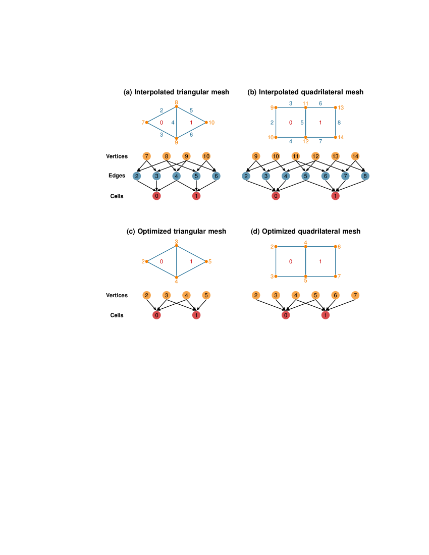
Figure 2: Direct acyclic graph representations of the covering relation for 2-D meshes with triangular and quadrilateral cells. The graphs for interpolated meshes (a) and (b) include all levels of the topology whereas the graphs for optimized meshes (c) and (d) only include the top and bottom levels. The graphs for interpolated meshes in 3-D include faces between edges and cells. PyLith currently uses the optimized graph representations.

The Sieve application programming interface (API) for mesh representation and manipulation is based upon a direct acyclic graph representation of the covering relation in a mesh, illustrated in Figure 2. For example, faces cover cells, edges cover faces, and points cover edges. By focusing on the key topological relations, the interface can be both concise and quite general. Using this generic API, PyLith is able to support one, two, and three dimensional meshes, with simplicial, hex, and even prismatic cell shapes, while using very little dimension or shape specific code. However, in order to include faults, we include additional operations in Sieve beyond those necessary for conventional finite-element operations.

In our domain decomposition approach, the finite-element mesh includes the fault as an interior surface. This forces alignment of the element faces along the fault. To impose a given fault slip as in equation (4), we must represent the displacement on both sides of the fault for any vertex on the fault. One option is to designate “fault vertices” which possess twice as many displacement DOF (Aagaard et al., 2001). However, this requires storing the global variable indices by cell rather than by vertex or adding special fault metadata to the vertices, significantly increasing storage costs and/or index lookup costs.

We choose another option and modify the initial finite-element mesh by replacing each fault face with a zero-volume cohesive cell. Many mesh generation tools do not support specification of faces on interior surfaces. Consequently, we create these cohesive cells in a preprocessing step at the beginning of a simulation. We construct the set of oriented fault faces from a set of vertices marked as lying on the fault. We join these vertices into faces, consistently orient them (using a common fault normal direction), and associate them with pairs of cells in the original mesh.

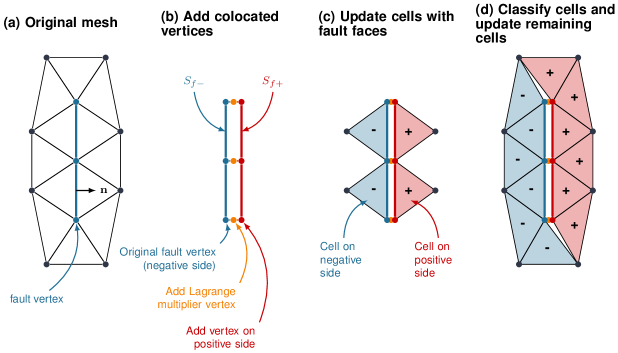
Figure 3: Construction of cohesive cells for a fault. (a) Original mesh with fault normal and fault vertices identified. (b) For each vertex on the fault, introduce a vertex on the positive side of the fault $S_{f^{+}}$ and a vertex corresponding to the Lagrange multiplier constraint between the pair of vertices on the positive and negative sides of the fault. (c) Identify cells with faces on the fault. Use the orientation of each face to identify cells on the positive and negative sides of the fault. Replace vertices in cells on the positive side of the fault with the newly created vertices. (d) Classify remaining cells with vertices on the fault using breadth-first search, and replace original vertices in cells on positive side of the fault with newly created vertices. Construct cohesive cells with zero volume from the vertices on the positive side of the fault, negative side of the fault, and Lagrange multiplier constraints.

Given this set of oriented fault faces, we introduce a set of cohesive cells using a step-by-step modification of the Sieve data structure representing the mesh illustrated in Figure 3. First, for each vertex on the negative side of the fault $S_{f^{-}}$, we introduce a second vertex on the positive side of the fault $S_{f^{+}}$ and a third vertex corresponding to the Lagrange multiplier constraint. The Lagrange multiplier vertex lies on an edge between the vertex on $S_{f^{+}}$ and the vertex on $S_{f^{-}}$. The fault faces are organized as a Sieve, and each face has the two cells it is associated with as descendants. Because the cells are consistently oriented, the first cell attached to each face is on the negative side of the fault, i.e., $S_{f^{-}}$. We replace the vertices on the fault face of each second cell, which is on the positive side of the fault, i.e., $S_{f^{+}}$, with the newly created vertices. Finally, we add a cohesive cell including the original fault face, a face with the newly created vertices, and the Lagrange vertices. These cohesive cells are prisms. For example, in a tetrahedral mesh the cohesive cells are triangular prisms, whereas in a hexahedral meshes they are hexahedrons.

We must also update all cells on the positive side of the fault that touch the fault with only an edge or single vertex. We need to replace the original vertices with the newly introduced vertices on the positive side of the fault. In cases where the fault reaches the boundaries of the domain, it is relatively easy to identify these cells because these vertices are shared with the cells that have faces on the positive side of the fault. However, in the case of a fault that does not reach the boundary of the domain, cells near the ends of the fault share vertices with cells that have a face on the positive side of the fault and cells that have a face on the negative side of the fault. We use a breadth-first classification scheme to classify all cells with vertices on the fault into those having vertices on the positive side of the fault and those having vertices on the negative side of the fault, so that we can replace the original vertices with the newly introduced vertices on the positive side of the fault.

In classifying the cells we iterate over the set of fault vertices. For each vertex we examine the set of cells attached to that vertex, called the support of the vertex in the Sieve API (Knepley and Karpeev, 2009). For each unclassified cell in the support, we look at all of its neighbors that touch the fault. If any is classified, we give the cell this same classification. If not, we continue with a breadth-first search of its neighbors until a classified cell is found. This search must terminate because there are a finite number of cells surrounding the vertex and at least one is classified (contains a face on the fault with this vertex). Depending on the order of the iteration, this can produce a “wrap around” effect at the ends of the fault, but it does not affect the numerical solution as long as the fault slip is forced to be zero at the edges of the fault. In prescribed slip simulations this is done via the user-specified slip distribution, whereas in spontaneous rupture simulations it is done by preventing slip with artificially large coefficients of friction, cohesive stress, or compressive normal tractions.

4 Solver Customization

4.1 Quasi-static Simulations

To solve the large, sparse systems of linear equations arising in our quasi-static simulations, we employ preconditioned Krylov subspace methods (Saad, 2003). We create a sequence of vectors by repeatedly applying the system matrix to the right-hand-side vector, $\bm{A^{k}}\cdot\bm{b}$, and they form a basis for a subspace, termed the Krylov space. We can efficiently find an approximate solution in this subspace. Because sparse matrix-vector multiplication is scalable via parallel processing, this is the method of choice for parallel simulation. However, for most physically relevant problems, the Krylov solver requires a preconditioner to accelerate convergence. While generic preconditioners exist (Saad, 2003; Smith et al., 1996), the method must often be specialized to a particular problem. In this section we describe a preconditioner specialized to our formulation for fault slip with Lagrange multipliers.

The introduction of Lagrange multipliers to implement the fault slip constraints produces the saddle-point problem shown in equation (24). Traditional black-box parallel preconditioners, such as the additive Schwarz Method (ASM) (Smith et al., 1996), are not very effective for this type of problem and produce slow convergence. However, PETSc provides tools to construct many variations of effective parallel preconditioners for saddle point problems.

The field split preconditioner in PETSc (Balay et al., 2010) allows the user to define sets of unknowns which correspond to different fields in the physical problem. This scheme is flexible enough to accommodate an arbitrary number of fields, mixed discretizations, fields defined over a subset of the mesh, etc. Once these fields are defined, a substantial range of preconditioners can be assembled using only PyLith options for PETSc. Table 1 shows example preconditioners and the options necessary to construct them.

Another option involves using the field split preconditioner in PETSc in combination with a custom preconditioner for the submatrix associated with the Lagrange multipliers. In formulating the custom preconditioner, we exploit the structure of the sparse Jacobian matrix. Our system Jacobian has the form

$$\bm{A}=\left(\begin{array}[]{cc}\bm{K}&\bm{L}^{T}\\ \bm{L}&\bm{0}\end{array}\right).$$ (41)

The Schur complement $\bm{S}$ of the submatrix $\bm{K}$ is given by,

$$\bm{S}=-\bm{L}\bm{K}^{-1}\bm{L}^{T}$$ (42)

which leads to a simple block diagonal preconditioner for $\bm{A}$

$$\bm{P}=\left(\begin{array}[]{cc}\bm{P}_{\mathit{elasticity}}&0\\ 0&\bm{P}_{\mathit{fault}}\end{array}\right)=\left(\begin{array}[]{cc}\bm{K}&0\\ 0&-\bm{L}\bm{K}^{-1}\bm{L}^{T}\end{array}\right).$$ (43)

The elastic submatrix $\bm{K}$, in the absence of boundary conditions, has three translational and three rotational null modes. These are provided to the algebraic multigrid (AMG) preconditioner, such as the ML library (Sala et al., 2004) or the PETSc GAMG preconditioner, to assure an accurate coarse grid solution. AMG mimics the action of traditional geometric multigrid, but it generates coarse level operators and interpolation matrices using only the system matrix, treated as a weighted graph, rather than a separate description of the problem geometry, such as a mesh. We split the elastic block from the fault block and also manage the Schur complements. In this way, all block preconditioners, including those nested with multigrid, can be controlled from the options file without recompilation or special code.

We now turn our attention to evaluating the fault portion of the preconditioning matrix associated with the Lagrange multipliers, since PETSc preconditioners can handle the elastic portion as discussed in the previous paragraph. In computing $\bm{P_{\mathit{fault}}}$ we approximate $\bm{K}^{-1}$ with the inverse of the diagonal portion of $\bm{K}$. Because $\bm{L}$ consists of integrating the products of basis functions over the fault faces, its structure depends on the quadrature scheme and the choice of basis functions. For conventional low order finite-elements and Gauss quadrature, $\bm{L}$ contains nonzero terms coupling the degree of freedom for each coordinate axes of a vertex with the corresponding degree of freedom of the other vertices in a cell. However, if we collocate quadrature points at the cell vertices, then only one basis function is nonzero at each quadrature point and $\bm{L}$ becomes block diagonal; this is also true for spectral elements with Legendre polynomials and Gauss-Lobatto-Legendre quadrature points. This leads to a diagonal matrix for the lower portion of the conditioning matrix,

$$\bm{P}_{\mathit{fault}}=-\bm{L}_{p}(\bm{K}_{n+n+}+\bm{K}_{n-n-})\bm{L}_{p}^{T},$$ (44)

where $\bm{L}_{p}$ is given in equation (25) and $\bm{K}_{n+n+}$ and $\bm{K}_{n-n-}$ are the diagonal terms from equation (26).

Our preferred setup uses the field splitting options in PETSc to combine an AMG preconditioner for the elasticity submatrix with our custom fault preconditioner for the Lagrange multiplier submatrix. See section 5 for a comparison of preconditioner performance for an application involving a static simulation with multiple faults. It shows the clear superiority of this setup over several other possible preconditioning strategies.

4.2 Dynamic Simulations

In dynamic simulations the Courant-Friderichs-Lewy condition (Courant et al., 1967) controls the stability of the explicit time integration. In most dynamic problems this dictates a relatively small time step so that a typical simulation involves tens of thousands of time steps. Hence, we want a very efficient solver to run dynamic simulations in a reasonable amount of time.

The Jacobian for our system of equations involves two terms: the inertial term given by equation (31) and the fault slip constraint term given by equation (23). Using conventional finite-element basis functions in these integrations results in a sparse matrix with off-diagonal terms. Although we can use the same solvers as we do for quasi-static simulations to find the solution, eliminating the off-diagonal terms so that the Jacobian is diagonal permits use of a much faster solver. With a diagonal Jacobian the number of operations required for the solve is proportional to the number of DOF, and the memory requirements are greatly reduced by storing the diagonal of the matrix as a vector rather than as a sparse matrix. However, the block structure of our Jacobian matrix, with the fault slip constraints occupying off-diagonal blocks, requires a two step approach to solve the linear system of equations without forming a sparse matrix.

First, we eliminate the off-diagonal entries in each block of the matrix during the finite-element integrations. The current best available option for eliminating the off-diagonal terms formed during the integration of the inertial term focuses on choosing a set of orthogonal basis functions, such as the Legendre polynomials with Gauss-Lobatto-Legendre quadrature points (Komatitsch and Vilotte, 1998). This discretization (often called the spectral element method) naturally produces a diagonal block for each finite-element cell without introducing any additional approximations. Because the fault slip constraint term also involves integration of the products of the basis functions over lower-dimension cells, orthogonal basis functions also produce a diagonal block for this integration.

In contrast, traditional finite-element approaches do introduce additional approximations when constructing a diagonal approximation. In PyLith we employ one of these traditional approaches, because it produces good approximations for many different choices of basis functions and quadrature points. For each finite-element cell, we construct a diagonal approximation of the integral such that the action on rigid body motion is the same for the diagonal approximation of the integral as it is for the original integral,

$$\bm{A}\cdot\bm{u}_{\mathrm{rigid}}=\bm{A}_{\mathit{diagonal}}\cdot\bm{u}_{\mathrm{rigid}}.$$ (45)

Expressing the diagonal block of the Jacobian matrix as a vector and the matrix of basis functions as a vector we have,

$$\bm{A}=\int_{\Omega}\bm{N}^{T}\cdot\bm{N}\,d\Omega\rightarrow\bm{A}_{\mathit{diagonal}}=\int_{\Omega}\bm{N}\sum_{i}N_{i}\,d\Omega,$$ (46)

where $N_{i}$ is the scalar basis function for degree of freedom $i$ and $\Omega$ may be the domain volume (as in the case of the inertial term) or a boundary (as in the case of the fault slip constraint term).

The errors associated with this approximation are small as long as the deformation occurs at length scales significantly larger than the discretization size, which is consistent with resolving seismic wave propagation accurately. Furthermore, in contrast to other approaches that choose basis functions or quadrature points that affect the accuracy of all of the finite-element integrations, such as choosing quadrature points coincident with the vertices of a cell, this approach only affects the accuracy of the terms involved in the Jacobian. For consistency in the formulation of the system of equations, these approximations are also applied to the inertial term and fault slip constraint term when computing the residual.

Second, we leverage the structure of the off-diagonal blocks associated with the fault slip constraint in solving the system of equations via a Schur’s complement algorithm. We compute an initial residual assuming the increment in the solution is zero (i.e., $\bm{du}_{n}=\bm{0}$ and $\bm{dl}_{p}=\bm{0}$),

$$\bm{r}^{*}=\begin{pmatrix}\bm{r}_{n}^{*}\\ \bm{r}_{p}^{*}\end{pmatrix}=\begin{pmatrix}\bm{b}_{n}\\ \bm{b}_{p}\end{pmatrix}-\begin{pmatrix}\bm{K}&\bm{L}^{T}\\ \bm{L}&0\end{pmatrix}\begin{pmatrix}\bm{u}_{n}\\ \bm{l}_{p}\end{pmatrix}.$$ (47)

We compute a corresponding initial solution to the system of equations $\bm{du}_{n}^{*}$ ignoring the off-diagonal blocks in the Jacobian and the increment in the Lagrange multipliers.

$$\bm{du}_{n}^{*}=\bm{K}^{-1}\cdot\bm{r}_{n},$$ (48)

taking advantage of the fact that we construct $\bm{K}$ so that it is diagonal.

We next compute the increment in the Lagrange multipliers to correct this initial solution so that the true residual is zero. Making use of the initial residual, the expression for the true residual is

$$\bm{r}=\begin{pmatrix}\bm{r}_{n}\\ \bm{r}_{p}\end{pmatrix}=\begin{pmatrix}\bm{r}_{n}^{*}\\ \bm{r}_{p}^{*}\end{pmatrix}-\begin{pmatrix}\bm{K}&\bm{L}^{T}\\ \bm{L}&0\end{pmatrix}\begin{pmatrix}\bm{du}_{n}\\ \bm{dl}_{p}\end{pmatrix}.$$ (49)

Solving the first row of equation (49) for the increment in the solution and accounting for the structure of $\bm{L}$ as we write the expressions for DOF on each side of the fault, we have

$$\bm{du}_{n^{+}}=\bm{du}_{n^{+}}^{*}-\bm{K}_{n^{+}n^{+}}^{-1}\cdot\bm{L}_{p}^{T}\cdot\bm{dl}_{p},$$ (50)

$$\bm{du}_{n^{-}}=\bm{du}_{n^{-}}^{*}+\bm{K}_{n^{-}n^{-}}^{-1}\cdot\bm{L}_{p}^{T}\cdot\bm{dl}_{p}.$$ (51)

Substituting into the second row of equation (49) and isolating the term with the increment in the Lagrange multipliers yields

$$\bm{L}_{p}\cdot\left(\bm{K}_{n^{+}n^{+}}^{-1}+\bm{K}_{n^{-}n^{-}}^{-1}\right)\cdot\bm{L}^{T}_{p}\cdot\bm{dl}_{p}=-\bm{r}_{p}^{*}+\bm{L}_{p}\cdot\left(\bm{du}_{n^{+}}^{*}-\bm{du}_{n^{-}}^{*}\right).$$ (52)

Letting

$$\bm{S}_{p}=\bm{L}_{p}\cdot\left(\bm{K}_{n^{+}n^{+}}^{-1}+\bm{K}_{n^{-}n^{-}}^{-1}\right)\cdot\bm{L}^{T}_{p},$$ (53)

and recognizing that $\bm{S}_{p}$ is diagonal because $\bm{K}$ and $\bm{L}_{p}$ are diagonal allows us to solve for the increment in the Lagrange multipliers,

$$\bm{dl}_{p}=\bm{S}_{p}^{-1}\cdot\left[-\bm{r}_{p}^{*}+\bm{L}_{p}\cdot\left(\bm{du}_{n^{+}}^{*}-\bm{du}_{n^{-}}^{*}\right)\right].$$ (54)

Now that we have the increment in the Lagrange multipliers, we can correct our initial solution $\bm{du}_{n}^{*}$ so that the true residual is zero,

$$\bm{du}_{n}=\bm{du}_{n}^{*}-\bm{K}^{-1}\cdot\bm{L}^{T}\cdot\bm{dl}_{p}.$$ (55)

Because $\bm{K}$ and $\bm{L}$ are comprised of diagonal blocks, this expression for the updates to the solution are local to the DOF attached to the fault and the Lagrange multipliers.

We also leverage the elimination of off-diagonal entries from the blocks of the Jacobian in dynamic simulations when updating the slip in spontaneous rupture models. Because $\bm{K}$ is diagonal in this case, the expression for the change in slip for a perturbation in the Lagrange multipliers (equations (36)–(38)) simplifies to

$$\partial\bm{d}_{p}=-\left(\bm{K}_{n^{+}n^{+}}^{-1}+\bm{K}_{n^{-}n^{-}}^{-1}\right)\cdot\bm{L}_{p}^{T}\cdot\partial\bm{l}_{p}.$$ (56)

Consequently, the increment in fault slip and Lagrange multipliers for each vertex can be done independently. In dynamic simulations the time step is small enough that the fault constitutive model is much less sensitive to the slip than in most quasi-static simulations, so we avoid performing a line search in computing the update.

5 Performance Benchmark

We compare the relative performance of the various preconditioners discussed in section 4.1 for quasi-static problems using a static simulation with three vertical, strike-slip faults. Using multiple, intersecting faults introduces multiple saddle points, so it provides a more thorough test of the preconditioner compared to a single fault with a single saddle point. Figure 4 shows the geometry of the faults embedded in the domain and Table 2 gives the parameters used in the simulation. We apply Dirichlet boundary conditions on two lateral sides with 2.0 m of shearing motion and no motion perpendicular to the boundary. We also apply a Dirichlet boundary condition to the bottom of the domain to prevent vertical motion. We prescribe uniform slip on the three faults with zero slip along the buried edges.

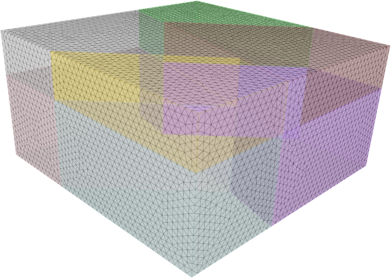
Figure 5: Tetrahedral finite-element mesh with a uniform discretization size of 1744 m for the performance benchmark. The colors correspond to the volumes in the CUBIT geometry that are separated by the fault surfaces and boundary between the upper crust and lower crust.

We generate both hexahedral meshes and tetrahedral meshes using CUBIT (available from http://cubit.sandia.gov) and construct meshes so that the problem size (number of DOF) for the two different cell types (hexahedra and tetrahedra) are nearly the same (within 2%). The suite of simulations examines increasingly larger problem sizes as we increase the number of processes (with one process per core), with $7.8\times 10^{4}$ DOF for 1 process up to $7.1\times 10^{6}$ DOF for 96 processes. The corresponding discretization sizes are 2033 m to 437 m for the hexahedral meshes and 2326 m to 712 m for the tetrahedral meshes. Figure 5 shows the 1846 m resolution tetrahedral mesh. As we will see in section 6.1, the hexahedral mesh for a given resolution in a quasi-static problem is slightly more accurate, so the errors in solution for each pair of meshes are larger for the tetrahedral mesh.

5.1 Preconditioner Performance

We characterize preconditioner performance in terms of the number of iterations required for the residual to reach a given convergence tolerance and the sensitivity of the number of iterations to the problem size. Of course, we also seek a minimal overall computation time. We examine the computation time in the next section when discussing the parallel performance. An ideal preconditioner would yield a small, constant number of iterations independent of problem size. However, for complex problems such as elasticity with fault slip and potentially nonuniform physical properties, ideal preconditioners may not exist. Hence, we seek a preconditioner that provides a minimal increase in the number of iterations as the problem size increases, so that we can efficiently simulate quasi-static crustal deformation related to faulting and post-seismic and interseismic deformation.

For this benchmark of preconditioner performance, we examine the number of iterations required for convergence using the PETSc additive Schwarz (ASM), field split (with and without our custom preconditioner), and Schur complement preconditioners discussed in section 4.1. We characterize the dependence on problem size using serial simulations (we examine parallel scaling for the best preconditioner in the next section) and the three lowest resolution meshes in our suite of hexahedral and tetrahedral meshes with the results summarized in Table 3.

The Schur complement and family of field split preconditioners using algebraic multigrid methods minimize the increase in the number of iterations with problem size. For these preconditioners the number of iterations increases by only about 20% for a four times increase in the number of degrees of freedom, compared to 60% for the ASM preconditioner. Within the family of field split preconditioners using algebraic multigrid methods, the one with multiplicative composition minimizes the number of iterations. The custom preconditioner for the Lagrange multiplier submatrix greatly accelerates the convergence with an 80% reduction in the number of iterations required for convergence. This preconditioner also provides the fastest runtime of all of these preconditioners.

5.2 Parallel Scaling Performance

The underlying PETSc solver infrastructure has demonstrated optimal scalability on the largest machines available today (Smith et al., 2008; Kaushik et al., 2009; Mills et al., 2010; Brown et al., 2012). However, computer science scalability results are often based upon unrealistically simple problems which do not advance the scientific state-of-the-art. In evaluating the parallel scalability of PyLith, we consider the sources responsible for reducing the scalability and propose possible steps for mitigation.

The main impediment to scalability in PyLith is load imbalance in solving the linear system of equations. This imbalance is the combination of three effects: the inherent imbalance in partitioning an unstructured mesh, partitioning based on cells rather than DOF, and weighting the cohesive cells the same as conventional bulk cells while partitioning. In this performance benchmark matrix-vector multiplication (the PETSc MatMult function) has a load imbalance of up to 20% on 96 cores. The cell partition balances the number of cells across the processes using ParMetis (Karypis et al., 1999) to achieve good balance for the finite element integration. This does not take into account a reduction in the number of DOF associated with constraints from Dirichlet boundary conditions or the additional DOF associated with the Lagrange multiplier constraints, which can exacerbate any imbalance. Nevertheless, eliminating DOF associated with Dirichlet boundary conditions preserves the symmetry of the overall systems and, in many cases, results in better conditioned linear systems.

We evaluate the parallel performance via a weak scaling criterion. That is, we run simulations on various numbers of processors/cores with an increase in the problem size as the number of processes increases (with one process per core) to maintain the same workload (e.g., number of cells and number of DOF) for each core. In ideal weak scaling the time for the various stages of the simulation is independent of the number of processes. For this performance benchmark we use the entire suite of hexahedral and tetrahedral meshes described earlier that range in size from $7.8\times 10^{4}$ DOF (1 process) to $7.1\times 10^{6}$ DOF (96 processes). We employ the AMG preconditioner for the elasticity submatrix and our custom preconditioner for the Lagrange multipliers submatrix. We ran the simulations on Lonestar at the Texas Advanced Computing Center. Lonestar is comprised of 1888 compute nodes connected by QDR Infiniband in a fat-tree topology, where each compute node consists of two six-core Intel Xeon E5650 processors with 24 GB of RAM. Simulations run on twelve or fewer cores were run on a single compute node with processes distributed across processors and then cores. For example, the two process simulation used one core on each of two processors. In addition to algorithm bottlenecks, runtime performance is potentially impeded by core/memory affinity, memory bandwidth, communication among compute nodes (including communication from other jobs running on the machine).

The single node scaling for PyLith (twelve processes or less in this case) is almost completely controlled by the available memory bandwidth. Good illustrations of the memory system performance are given by the VecAXPY, VecMAXPY and VecMDot operations reported in the log summary (Balay et al., 2010). These operations are limited by available memory bandwidth rather than the rate at which a processor or core can perform floating points operations. From Table 4, we see that we saturate the memory bandwidth using two processes (cores) per processor, since scaling plateaus from 2 to 4 processes, but shows good scaling from 12 to 24 processes. This lack of memory bandwidth will depress overall performance, but should not affect the inter-node scaling of the application.

Machine network performance can be elucidated by the VecMDot operation for vector reductions, and MatMult for point-to-point communication. In Table 4 we see that the vector reduction shows good scaling up to 96 processes. Similarly in Table 5, we see that MatMult has good scalability, but that it is a small fraction of the overall solver time. The AMG preconditioner setup (PCSetUp) and application (PCApply) dominate the overall solver time. The AMG preconditioner setup time increases with the number of processes. Note that many weak scaling studies do not include this event, because it is amortized over the iteration. Nevertheless, in our benchmark it is responsible for most of the deviation from perfect weak scaling. We could trade preconditioner strength for scalability by reducing the work done on the coarse AMG grids, so that the solver uses more iterations which scale very well. However, that would increase overall solver time and thus would not be the choice to maximize scientific output.

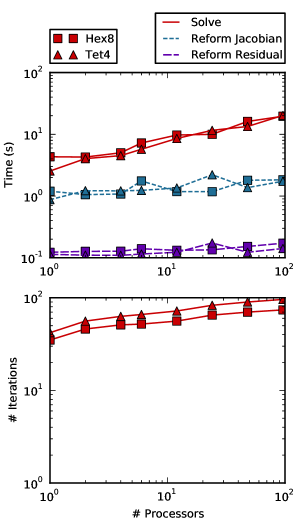
Figure 6: Plot of parallel scaling for the performance benchmark with the algebraic multigrid preconditioner and fault block custom preconditioner. The stages shown include the numerical integration of the residual (Reform Residual) and Jacobian (Reform Jacobian) and setting up the preconditioner and solving the linear system of equations (Solve). The finite-element integrations for the Jacobian and residual exhibit good weak scaling with minimal sensitivity to the problem size. The linear solve (solid lines in the top panel) does not scale as well, which we attribute to the poor scaling of the algebraic multigrid setup and application as well as limited memory and interconnect bandwidth. We attribute fluctuations in the relative performance to variations in the machine load from other jobs on the cluster.

Figure 6 illustrates the excellent parallel performance for the finite-element assembly routines (reforming the Jacobian sparse matrix and computing the residual). As discussed earlier in this section, the ASM preconditioner performance is not scalable because the number of iterations increases significantly with the number of processes. As shown in Figure 6, the introduction of Schur complement methods and an AMG preconditioner slows the growth considerably, and future work will pursue the ultimate goal of iteration counts independent of the number of processes.

6 Code Verification Benchmarks

In developing PyLith we verify the numerical implementation of various features using a number of techniques. We employ unit testing to verify correct implementation of nearly all of the individual routines. Having a test for most object methods or functions isolates bugs at their origin during code development and prevents new bugs from occurring as code is modified or optimized. We also rely on full-scale benchmarks to verify that the code properly solves the numerical problem. These benchmarks include quasi-static strike-slip and reverse viscoelastic simulations and various exercises in the suite of dynamic spontaneous rupture benchmarks developed by the Southern California Earthquake Center (SCEC) and the United States Geological Survey (Harris et al., 2009). The mesh generation and simulation parameter files for many of the benchmarks, including those discussed here, are available from the CIG subversion repository (http://geodynamics.org/svn/cig/short/3D/PyLith/benchmarks/trunk/). In this section we focus on two benchmarks that test different scientific applications: quasi-static relaxation of a Maxwell viscoelastic material subjected to multiple earthquake cycles involving slip and steady creep on a vertical strike-slip fault (Savage and Prescott, 1978) and supershear dynamic spontaneous rupture of a 60 degree dipping normal fault in a Drucker-Prager elastoplastic medium. This second benchmark corresponds to benchmark TPV13 in the SCEC suite of dynamic spontaneous rupture benchmarks (Harris et al., 2011).

6.1 Quasi-static Benchmark

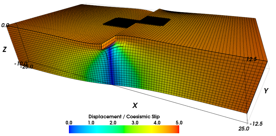
Figure 7: Deformation (exaggerated by a factor of 5000) 95% of the way through earthquake cycle 10 of the Savage and Prescott benchmark, which involves viscoelastic relaxation over multiple earthquake cycles on a vertical, strike-slip fault. The coordinates are in units of elastic layer thickness and the displacement field is in units of coseismic slip. The locking depth is one-half of the thickness of the elastic layer. We refine the hexahedral mesh by a factor of three near the center of the domain. Figure 8 compares profiles along y=0 with the analytic solution.

As a test of our quasi-static solution, we compare our numerical results against the analytical solution of Savage and Prescott (1978). This problem consists of an infinitely long strike-slip fault in an elastic layer overlying a Maxwell viscoelastic half-space. The parameter files for this benchmark are available in the quasistatic/sceccrustdeform/savageprescott directory of the benchmark repository. Figure 7 illustrates the geometry of the problem with an exaggerated view of the deformation during the tenth earthquake cycle. Between earthquakes the upper portion of the fault is locked, while the lower portion slips at the plate velocity. At regular intervals (the earthquake recurrence time) the upper portion of the fault slides such that the slip on the locked portion exactly complements the slip on the creeping portion so the cumulative slip over an earthquake cycle is uniform.

This problem tests the ability of the kinematic fault implementation to include steady aseismic creep and multiple earthquake ruptures along with viscoelastic relaxation. The analytical solution for this problem provides the along-strike component of surface displacement as a function of distance perpendicular to the fault. The solution is controlled by the ratio of the fault locking depth to the thickness of the elastic layer and the ratio of the earthquake recurrence time to the viscoelastic relaxation time, $\tau_{0}=\mu T/2\eta$, where $T$ is the recurrence time, $\mu$ is the shear modulus and $\eta$ is the viscosity.

For this benchmark we use a locking depth of 20 km, an elastic layer thickness of 40 km, an earthquake recurrence time of 200 years, a shear modulus of 30 GPa, a viscosity of $2.37\times 10^{19}$ Pa-s, and a relative plate velocity of 2 cm/year, implying a coseismic offset of 4 m every 200 years (see Table 6). The viscosity and shear modulus values yield a viscoelastic relaxation time of 50 years, and $\tau_{0}=4$. We employ a 3-D model (2000 km by 1000 km by 400 km) with Dirichlet boundary conditions enforcing symmetry to approximate an infinitely long strike-slip fault. We apply velocity boundary conditions in the y-direction to the -x and +x faces with zero x-displacement. We constrain the vertical displacements on the bottom of the domain to be zero. Finally, we fix the x-displacements on the -y and +y faces to enforce symmetry consistent with an infinitely long strike-slip fault.

We examine four different numerical solutions considering the effects of cell type (hexahedral versus tetrahedral) and discretization size. In our coarse hexahedral mesh we use a uniform resolution of 20 km. In our higher resolution hexahedral mesh we refine an inner region (480 km by 240 km by 100 km) by a factor of three, yielding a resolution near the center of the fault of 6.7 km. For the tetrahedral meshes, we match the discretization size of the hexahedral mesh near the center of the fault (20km or 6.7 km) while increasing the discretization size in a geometric progression at a rate of 1.02. This results in a maximum discretization size of approximately 60 km for the coarser mesh and 40 km for the higher resolution mesh. Note that for both the hexahedral and tetrahedral coarse meshes, the discretization size on the fault is the maximum allowable size that still allows us to represent the fault locking depth as a sharp boundary.

In this viscoelastic problem neither the analytical or numerical models approach steady-state behavior until after several earthquake cycles. There is also a difference in how steady plate motion is applied for the two models. For the analytical solution, steady plate motion is simply superimposed, while for the numerical solution steady plate motion is approached after several earthquake cycles, once the applied fault slip and velocity boundary conditions have produced nearly steady flow in the viscoelastic half-space. It is therefore necessary to spin-up both solutions to their steady-state solution over several earthquake cycles to allow a comparison between the two. In this way, the transient behavior present in both models will have nearly disappeared, and both models will have approximately the same component of steady plate motion. We simulate ten earthquake cycles for both the analytical and numerical models for a total duration of 2000 years. For the numerical solution we use a constant time step size of five years. This time step corresponds to one tenth of the viscoelastic relaxation time; hence it tests the accuracy of the viscoelastic solution for moderately large time steps relative to the relaxation time. Recall that the quasi-static formulation does not include inertial terms and time stepping is done via a series of static problems so that the temporal accuracy depends only on the temporal variation of the boundary conditions and constitutive models. These benchmarks simulations can be run on a laptop or desktop computer. For example, the high resolution benchmarks took 46 min (hexahedral cells) and 36 min (tetrahedral cells) using four processes on a dual quad core desktop computer with Intel Xeon E5630 processors.

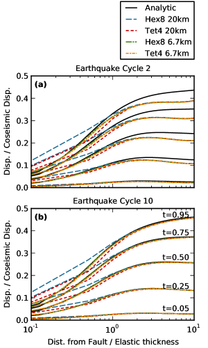
Figure 8: Comparison of displacement profiles perpendicular to the fault in the Savage and Prescott benchmark during earthquake cycles (a) two and (b) ten. The displacement values shown are relative to the values at the beginning of the earthquake cycle to facilitate comparison between the analytical solution and the numerical models. Both the analytical and numerical simulations require spin-up to reach the steady-state solution, and the numerical models also require spin-up to achieve steady plate motion, which is superimposed on the analytical solution. Both the hexahedral (Hex8) and tetrahedral (Tet4) discretizations resolve the viscoelastic deformation and display excellent agreement with the steady-state solution by the tenth earthquake cycle. The coarser (20 km) resolutions are unable to match the details of the displacement field at distances less than about one elastic thickness, but all of the numerical models provide a good fit to the analytical solution in the tenth earthquake cycle at distances greater than 2–3 times the elastic thickness.

Figure 8 compares the numerical results extracted on the ground surface along the center of the model perpendicular to the fault with the analytic solution. Using a logarithmic scale with distance from the fault facilitates examining the solution both close to and far from the fault. For the second earthquake cycle, the far-field numerical solution does not yet accurately represent steady plate motion and the numerical simulations underpredict the displacement. By the tenth earthquake cycle, steady plate motion is accurately simulated and the numerical results match the analytical solution.

Within about one elastic thickness of the fault the effect of the resolution of the numerical models becomes apparent. We find large errors for the coarse models, which have discretization sizes matching the fault locking depth. The finer resolution models (6.7 km discretization size) provide a close fit to the analytical solution. The 6.7 km hexahedral solution is indistinguishable from the analytical solution in Figure 8(b); the 6.7 km tetrahedral solution slightly underpredicts the analytical solution for times late in the earthquake cycle. The greater accuracy of the hexahedral cells relative to the tetrahedral cells with the same nominal discretization size for quasi-static solutions is consistent with our findings for other benchmarks. The greater number of polynomial terms in the basis functions of the hexahedra allows the model to capture a more complex deformation field at a given discretization size.

6.2 Dynamic Benchmark

As a test of PyLith’s dynamic spontaneous rupture solutions, we use SCEC Spontaneous Rupture Benchmark TPV13 that models a high stress-drop, supershear, dip-slip earthquake that produces extreme (very large) ground motions, large slip, and fast slip rates (Harris et al., 2011). It uses a Drucker-Prager elastoplastic bulk rheology and a slip-weakening friction model in a depth-dependent initial stress field. The parameter files for this benchmark are available in the dynamic/scecdynrup/tpv210-2d and dynamic/scecdynrup/tpv210 directories of the benchmark repository.

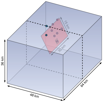
Figure 9: Geometry for SCEC spontaneous rupture benchmark TPV13 involving a Drucker-Prager elastoplastic bulk rheology, slip-weakening friction, a depth-dependent stress field, and normal fault with a 60 degree dip angle. The 2-D version corresponds to the vertical slice shown by the dashed line. The red dots denote locations on the fault used in the comparison of the vertical slip rates (Figures 12 and 14). The blue dots indicate locations on the ground surface used in the comparison of fault normal and vertical velocity time histories (Figure 15).

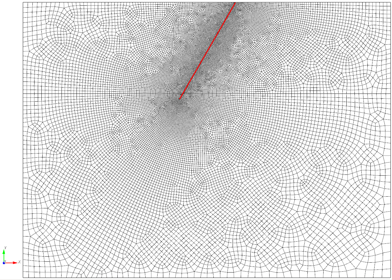
Figure 10: Finite-element mesh comprised of quadrilateral cells for SCEC spontaneous rupture benchmark TPV13-2D. The discretization size is 100 m on the fault surface and increases at a geometric rate of 2% with distance from the fault. We employ this same spatial variation of the discretization size in the 3-D model.

Figure 9 shows the geometry of the benchmark and the size of the domain we used in our verification test. The benchmark includes both 2-D (TPV13-2D is a vertical slice through the fault center-line with plane strain conditions) and 3-D versions (TPV13). This benchmark specifies a spatial resolution of 100 m on the fault surface. To examine the effects of cell type and discretization size we consider both triangular and quadrilateral discretizations with resolutions on the fault of 50 m, 100 m, and 200 m for TPV13-2D and 100 m and 200 m for TPV13. We gradually coarsen the mesh with distance from the fault by increasing the discretization size at a geometric rate of 2%. This provides high resolution at the fault surface to resolve the small scale features of the rupture process and less resolution at the edges of the boundary where the solution is much smoother. Figure 10 shows the triangular mesh for a discretization size of 100 m on the fault.

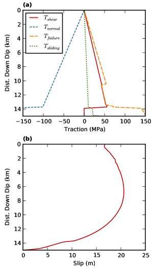
Figure 11: (a) Depth-dependent fault tractions in SCEC spontaneous rupture benchmark TPV13-2D and TPV13. $T_{\mathit{shear}}$ denotes the initial shear traction, $T_{\mathit{normal}}$ denotes the initial effective normal traction, $T_{\mathit{failure}}$ denotes the frictional failure stress corresponding to the initial effective normal traction, and $T_{\mathit{sliding}}$ denotes the dynamic sliding stress corresponding to the initial effective normal traction. Positive shear tractions correspond to normal faulting and negative normal tractions correspond to compression. (b) Final slip as a function of depth in TPV13-2D for the triangular mesh with a resolution of 100 m on the fault.

Rupture initiates due to a low static coefficient of friction in the nucleation region. Figure 11(a) illustrates the depth dependence of the stress field in terms of the fault tractions and Table 7 summarizes the benchmark parameters. Harris et al. (2011) provides a more complete description with all of the details available from http://scecdata.usc.edu/cvws/cgi-bin/cvws.cgi. A challenging feature of this, and many other benchmarks in the SCEC Spontaneous Rupture Code Verification Exercise, is the use of parameters with spatial variations that are not continuous. This includes the variation in the static coefficient of friction for the nucleation region and the transition to zero deviatoric stresses near the bottom of the fault. We impose the geometry of these discontinuities in the construction of the finite-element mesh and use the spatial average of the parameters where they are discontinuous. This decreases the sensitivity of the numerical solution to the discretization size. This SCEC benchmark also includes fluid pressures. Because PyLith does not include fluid pressure, we instead formulate the simulation parameters in terms of effective stresses.

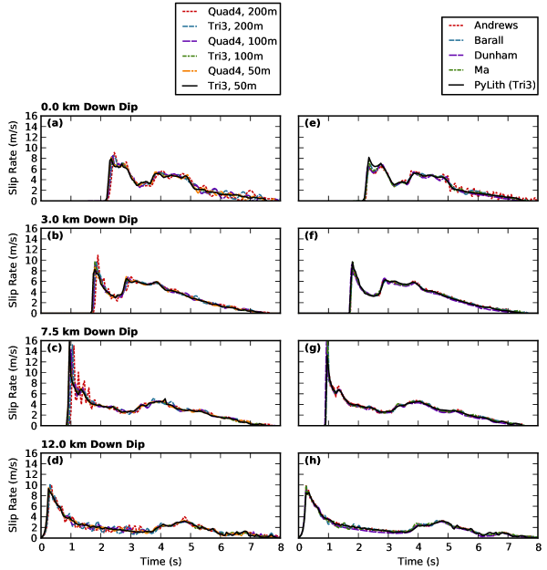
Figure 12: Slip rate time histories for SCEC spontaneous rupture benchmark TPV13-2D. Locations correspond to the red dots along the center-line of the fault shown in Figure 9. Panels (a)–(d) show convergence of the solution for quadrilateral and triangular cells as a function of discretization size, and panels (e)–(h) demonstrate of code verification via excellent agreement among PyLith and four other dynamic rupture modeling codes (Harris et al., 2011).

The TPV13-2D simulations require a small fraction of the computational resources needed for the TPV13 3-D simulations and run quickly on a laptop or desktop computer. The 50 m resolution cases took 62 s (triangular cells) and 120 s (quadrilateral cells) using 8 processes on a dual quad core desktop computer with Intel Xeon E5630 processors. Figure 11(b) displays the final slip distribution in the TPV13-2D simulation with triangular cells at a resolution of 100 m. The large dynamic stress drop and supershear rupture generate 20 m of slip at a depth of about 7 km. Figure 12(a)–(d) demonstrates the convergence of the solution as the discretization size decreases as evident in the normal faulting component of fault slip rate time histories. For a resolution of 200 m on the fault, the solution contains some high-frequency oscillation due to insufficient resolution of the cohesive zone (Rice, 1993). The finer meshes provide sufficient resolution of the cohesive zone so there is very little high-frequency oscillation in the slip rate time histories. The triangular cells generate less oscillation compared with quadrilateral cells.

In this benchmark without an analytical solution, as in all of the exercises in the SCEC spontaneous rupture benchmark suite, we rely on comparison with other dynamic spontaneous rupture modeling codes to verify the numerical implementation in PyLith. Figure 12(e)–(h) compares the slip rate time histories from PyLith with four other codes (see Harris et al. (2011), Andrews et al. (2007), Barall (2009), Ma (2009), and Dunham et al. (2011) for a discussion of these other finite-element and finite-difference codes). The slip rate time histories agree very well, although some codes yield more oscillation than others. We attribute this to variations in the amount of numerical damping used in the various codes.

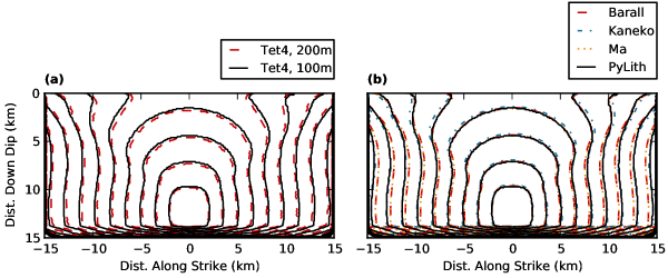
Figure 13: Rupture time contours (0.5 s interval) for SCEC spontaneous rupture benchmark TPV13. (a) Effect of discretization size and (b) demonstration of code verification via excellent agreement among PyLith and three other dynamic rupture modeling codes (Harris et al., 2011). The contours for PyLith and Kaneko (spectral element code) are nearly identical.

The 3-D version of the TPV13 benchmark yields similar results but requires greater computational resources. The simulations with a discretization size of 100 m took 2.5 hours using 64 processes (8 compute nodes with 8 processes per dual quad core compute node) on a cluster with Intel Xeon E5620 processors. Figure 13(a) shows the same trends in rupture speed with discretization size that we observed in the 2-D version. In both cases models with insufficient resolution to resolve the cohesive zone propagate slightly slower than models with sufficient resolution. In this case the differences between the rupture times for the 200 m and 100 m resolution tetrahedral meshes are less than 0.1 seconds over the entire fault surface. Comparing the rupture times among the modeling codes in Figure 13, we find that the four codes fall into two groups. In the mode-III (along-strike) direction, PyLith and the spectral element code by Kaneko et al. (2008) are essentially identical while the finite-element codes by Barall (2009) and Ma and Andrews (2010) are also essentially identical. In the mode-II (up-dip) direction all four codes agree very closely. As in the 2-D version, we attribute the differences among the codes not to the numerical implementation but the treatment of discontinuities in the spatial variation of the parameters. This explains why the higher-order spectral element code by Kaneko et al. (2008) agrees so closely with PyLith, a lower-order finite-element code.

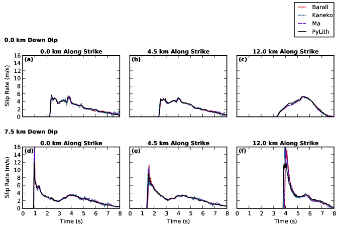
Figure 14: Comparison of normal faulting component of slip rate at six locations on the fault surface for SCEC spontaneous rupture benchmark TPV13. (a)–(c) are at a depth of 0 km and (d)–(f) are at a depth of 7.5 km. The slip rate time histories for all four dynamic rupture modeling codes agree very well. At 12 km along strike and 7.5 km down dip, there is a small discrepancy between two groups of codes (PyLith and Kaneko versus Barall and Ma) that we attribute to how the modelers handled the discontinuity in the initial stress field and parameters.

The slip rate and velocity time histories displayed in Figures 14 and 15 are consistent with the trends observed in the comparison of rupture times. Furthermore, the codes all produce consistent results throughout the entire time histories. The small differences in rupture time in the mode-III (along-strike) direction between the two groups of codes is evident in the slip rate time histories at a depth of 7.5 km and 12 km along strike (Figure 14(f)). Nevertheless, this simply produces a small time shift in the time history.

From the 2-D and 3-D versions of the SCEC spontaneous rupture benchmark TPV13, we conclude that PyLith performs similarly to other finite-element and finite-difference dynamic spontaneous rupture modeling codes. In particular it is well-suited to problems with complex geometry, as we are able to vary the discretization size while simulating a dipping normal fault. The code accurately captures supershear rupture and properly implements a Drucker-Prager elastoplastic bulk rheology and slip-weakening friction.

7 Conclusions

PyLith provides a flexible numerical implementation of fault slip using a domain decomposition approach. We have evaluated the efficiency of several preconditioners for use of this fault implementation in quasi-static simulations. We find that algebraic multigrid preconditioners for elasticity combined with a custom preconditioner for the fault block associated with the Lagrange multipliers accelerates the convergence of the Krylov solver with the fewest number of iterations and the least sensitivity to problem size. Benchmark tests demonstrate the accuracy of our fault slip implementation in PyLith with excellent agreement to (1) an analytical solution for viscoelastic relaxation and strike-slip faulting over multiple earthquake cycles and (2) other codes for supershear dynamic spontaneous rupture on a dipping normal fault embedded in an elastoplastic domain. Consequently, we believe this methodology provides a promising avenue for modeling the earthquake cycle through coupling of quasi-static simulations of the interseismic and postseismic deformation and dynamic rupture simulations of earthquake rupture propagation.

$\bm{A}$ & matrix associated with Jacobian operator for the entire system of equations.
$\bm{C}$ fourth order tensor of elastic constants.
$\bm{d}$ fault slip vector.
$\bm{f}$ body force vector.
$\bm{l}$ Lagrange multiplier vector corresponding to the fault traction vector.
$\bm{L}$ matrix associated with Jacobian operator for constraint equation.
$\bm{K}$ matrix associated with Jacobian operator for elasticity equation.
$\bm{N}_{m}$ matrix for $m$ basis functions.
$\bm{n}$ normal vector.
$\bm{P}$ preconditioning matrix.
$\bm{P}_{\mathit{elastic}}$ preconditioning matrix associated with elasticity.
$\bm{P}_{\mathit{fault}}$ preconditioning matrix associated with fault slip constraints (Lagrange multipliers).
$S_{f}$ fault surface.
$S_{T}$ surface with Neumann boundary conditions.
$S_{u}$ surface with Dirichlet boundary conditions.
$t$ time.
$\bm{T}$ Traction vector.
$T_{c}$ scalar shear traction associated with cohesion.
$T_{f}$ scalar shear traction associated with friction.
$T_{n}$ scalar normal traction.
$\bm{u}$ displacement vector.
$V$ spatial domain of model.
$V_{p}$ dilatational wave speed.
$V_{s}$ shear wave speed.
$\Delta t$ time step.
$\eta^{*}$ nondimensional viscosity used for numerical damping.
$\boldsymbol{\phi}$ weighting function.
$\mu_{f}$ coefficient of friction.
$\rho$ mass density.
$\bm{\sigma}$ Cauchy stress tensor.

Figure 1: Diagram of domain decomposition approach for modeling fault slip. The fault slip introduces a jump in the displacement field across the fault, whereas the tractions are continuous.

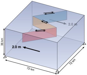
Figure 4: Geometry of problem used in quasi-static performance benchmark. Dirichlet boundary conditions prescribe a horizontal lateral displacement of 2.0 m with no motion normal to the boundary on two sides of the domain and zero vertical displacement on the bottom boundary. We specify uniform slip of 1.0 m of right-lateral motion on the middle fault and 0.5 m of left-lateral motion on the two other faults. The faults extend down to a depth of 12.0 km.

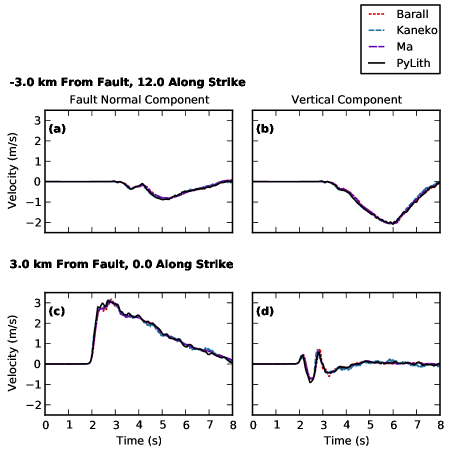
Figure 15: Comparison of fault normal and vertical components of velocity time histories at two sites on the ground surface for SCEC spontaneous rupture benchmark TPV13. Panels (a)–(b) are associated with a site that is on the hanging wall 3 km from the fault trace and 12 km along strike, and panels (c)–(d) are associated with a site that is on the footwall 3 km from the fault trace along the fault center-line. As expected based on the close agreement in the rupture time contours and fault slip rates, the velocity time histories from the difference dynamic rupture modeling codes agree very closely.

Table 1: Example Preconditioners for the Saddle Point Problem in Equation (24)a

AMG with additive relaxation	AMG with multiplicative relaxation
$\begin{pmatrix}\bm{K}&\bm{0}\\ \bm{0}&\bm{I}\end{pmatrix}$	$\begin{pmatrix}\bm{K}&\bm{L}^{T}\\ \bm{0}&\bm{I}\end{pmatrix}$
[pylithapp.problem.formulation]	[pylithapp.problem.formulation]
split_fields = True	split_fields = True
matrix_type = aij	matrix_type = aij
[pylithapp.petsc]	[pylithapp.petsc]
fs_pc_type = fieldsplit	fs_pc_type = fieldsplit
fs_pc_field_split_real_diagonal = true	fs_pc_field_split_real_diagonal = true
fs_pc_field_split_type = additive	fs_pc_field_split_type multiplicative
fs_fieldsplit_0_pc_type = ml	fs_fieldsplit_0_pc_type = ml
fs_fieldsplit_0_ksp_type = preonly	fs_fieldsplit_0_ksp_type = preonly
fs_fieldsplit_1_pc_type = jacobi	fs_fieldsplit_1_pc_type = jacobi
fs_fieldsplit_1_ksp_type = gmres	fs_fieldsplit_1_ksp_type = gmres
Schur complement, upper factorization	Schur complement, full factorization
$\begin{pmatrix}\bm{K}&\bm{L}^{T}\\ \bm{0}&\bm{S}\end{pmatrix}$	$\begin{pmatrix}\bm{I}&\bm{0}\\ \bm{B}^{T}\bm{A}^{-1}&\bm{I}\end{pmatrix}\begin{pmatrix}\bm{A}&\bm{0}\\ \bm{0}&\bm{S}\end{pmatrix}\begin{pmatrix}\bm{I}&\bm{A}^{-1}\bm{B}\\ \bm{0}&\bm{I}\end{pmatrix}$
[pylithapp.problem.formulation]	[pylithapp.problem.formulation]
split_fields = True	split_fields = True
matrix_type = aij	matrix_type = aij
[pylithapp.petsc]	[pylithapp.petsc]
pc_type = fieldsplit	pc_type = fieldsplit
pc_field_split_type = schur	pc_field_split_type = schur
fs_pc_field_split_real_diagonal = true	fs_pc_field_split_real_diagonal = true
pc_fieldsplit_schur_factorization_type = upper	pc_fieldsplit_schur_factorization_type = full
pc_fieldsplit_schur_precondition = user	pc_fieldsplit_schur_precondition = user
fieldsplit_0_pc_type = ml	fieldsplit_0_pc_type = ml
fieldsplit_0_ksp_type = preonly	fieldsplit_0_ksp_type = preonly
fieldsplit_1_pc_type = jacobi	fieldsplit_1_pc_type = jacobi
fieldsplit_1_ksp_type = gmres	fieldsplit_1_ksp_type = gmres

aFour examples of preconditioners often used to accelerate convergence in saddle point problems. Below the mathematical expression for the preconditioner, we show the PyLith parameters used to construct the preconditioner.

Table 2: Performance Benchmark Parametersa

Parameter		Value
Domain
	Length	72 km
	Width	72 km
	Height	36 km
	Angle between faults	60 $\deg$
Elastic properties
	Vp	5.774 km/s
	Vs	3.333 km/s
	Density ($\rho$)	2700. kg/m3
Middle fault
	Length	39.19 km
	Width	12 km
	Slip	1.0 m RL
End faults
	Length	43.74 km
	Width	12 km
	Slip	0.5 m LL

aSimulation parameters for the performance benchmark with three faults embedded in a volume domain as shown in Figure 4. We prescribe right-lateral (RL) slip on the middle fault and left-lateral (LL) slip on the end faults.

Table 3: Preconditioner Performancea

Preconditioner	Cell	Problem Size
		S1	S2	S4
ASM	Tet4	184	217	270
	Hex8	143	179	221
Schur (full)	Tet4	82	84	109
	Hex8	54	60	61
Schur (upper)	Tet4	79	78	87
	Hex8	53	59	57
FieldSplit (add)	Tet4	241	587	585
	Hex8	159	193	192
FieldSplit (mult)	Tet4	284	324	383
	Hex8	165	177	194
FieldSplit (mult,custom)	Tet4	42	48	51
	Hex8	35	39	43

aNumber of iterations for additive Schwarz (ASM), Schur complement (Schur), and field split (additive, multiplicative, and multiplicative with custom fault block preconditioner), preconditioners for tetrahedral and hexahedral discretizations and three problem sizes (S1 with $1.8\times 10^{5}$ DOF, S2 with $3.5\times 10^{5}$ DOF, and S3 with $6.9\times 10^{5}$ DOF). The Schur complement preconditioners and the field split preconditioner with multiplicative factorization and the custom fault block preconditioner yield the best performance with only a fraction of the iterates as the other preconditioners and a small increase with problem size. Furthermore, the field split preconditioner with multiplicative factorization and the custom fault block preconditioner provides the shortest runtime.

Table 4: Performance Benchmark Memory System Evaluationa

Event	# Cores	Load Imbalance	MFlops/s
VecMDot	1	1.0	2007
	2	1.1	3809
	4	1.1	5431
	6	1.1	5967
	12	1.2	5714
	24	1.2	11784
	48	1.2	20958
	96	1.3	17976
VecAXPY	1	1.0	1629
	2	1.1	3694
	4	1.1	5969
	6	1.1	6028
	12	1.2	5055
	24	1.2	10071
	48	1.2	18761
	96	1.3	33676
VecMAXPY	1	1.0	1819
	2	1.1	3415
	4	1.1	5200
	6	1.1	5860
	12	1.2	6051
	24	1.2	12063
	48	1.2	23072
	96	1.3	28461

aExamination of memory system performance using three PETSc vector operations for simulations with the hexahedral meshes. The performance for the tetrahedral meshes is very similar. For ideal scaling the number of floating point operations per second should scale linearly with the number of processes. VecMDot corresponds to the operation for vector reductions, VecAXPY corresponds to vector scaling and addition, and VecMAXPY corresponds to multiple vector scaling and addition.

Table 5: Performance Benchmark Solver Evaluationa

Event	# Calls	Time (s)	MFlops/s
p = 12
MatMult	180	2.7	6113
PCSetUp	1	5.7	232
PCApply	57	5.5	3690
KSPSolve	1	15.1	3013
p = 24
MatMult	207	3.1	12293
PCSetUp	1	5.2	526
PCApply	66	6.6	7285
KSPSolve	1	16.4	6666
p = 48
MatMult	222	4.0	21136
PCSetUp	1	10.1	628
PCApply	71	9.4	12032
KSPSolve	1	25.1	10129
p = 96
MatMult	234	4.0	42130
PCSetUp	1	11.8	1943
PCApply	75	11.6	20422
KSPSolve	1	30.5	17674

aExamination of solver performance using three of the main events comprising the linear solve for simulations with the hexahedral meshes and 12, 24, 48, and 96 processes. The performance for the tetrahedral meshes is nearly the same. For ideal scaling the time for each event should be constant as the number of processes increases. The KSPSolve event encompasses the entire linear solve. MatMult corresponds to matrix-vector multiplications. PCSetUp and PCApply correspond to the setup and application of the AMG preconditioner.

Table 6: Savage and Prescott Benchmark Parametersa

Parameter		Value
Domain
	Length	2000 km
	Width	1000 km
	Height	400 km
	Fault dip angle	90 $\deg$
Physical properties
	Shear modulus	30 GPa
	Viscosity	$2.37\times 10^{19}$ Pa-s
	Elastic thickness	40 km
Fault slip
	Locking depth	20 km
	Earthquake recurrence	200 yr
	Earthquake slip	4 m
	Creep rate	2 cm/yr

aSimulation parameters for the Savage and Prescott benchmark with multiple earthquake cycles on a vertical strike-slip fault embedded in an elastic layer over a viscoelastic half-space.

Table 7: SCEC Benchmark TPV13 Parametersa

Parameter		Value
Domain
	Length	64 km
	Width	48 km
	Height	36 km
	Fault dip angle	60 $\deg$
Elastic properties
	Vp	5.716 km/s
	Vs	3.300 km/s
	Density ($\rho$)	2700. kg/m3
	Nondimensional viscosity ($\eta^{*}$)	0.4

aBasic simulation parameters for the SCEC dynamic spontaneous rupture benchmark TPV13. A complete list of the parameters can be found in Harris et al. (2011).