A Probabilistic Model for LCF

Abstract

Fatigue life of components or test specimens often exhibit a significant scatter. Furthermore, size effects have a non-negligible influence on fatigue life of parts with different geometries. We present a new probabilistic model for low-cycle fatigue (LCF) in the context of polycrystalline metal. The model takes size effects and inhomogeneous strain fields into account by means of the Poisson point process (PPP). This approach is based on the assumption of independently occurring LCF cracks and the Coffin-Manson-Basquin (CMB) equation. Within the probabilistic model, we give a new and more physical interpretation of the CMB parameters which are in the original approach no material parameters in a strict sense, as they depend on the specimen geometry. Calibration and validation of the proposed model is performed using results of strain controlled LCF tests of specimens with different surface areas. The test specimens are made of the nickel base superalloy RENE 80.

1 Introduction

In fatigue analysis, standardized specimen tests are commonly used to represent temperature and stress conditions in engineering parts under cyclic loading. Results of these tests are usually visualized in E - N and S - N diagrams (Wöhler curves) for strain and stress controlled fatigue, respectively. Within the safe-life approach of fatigue design, these diagrams are employed to predict the fatigue life of engineering parts. In addition, safety factors are applied to take the scatter for fatigue life, size effects and uncertainties in the stress and temperature fields into account. In contrast to that, in a probabilistic approach, these quantities are explicitly taken into account: In the present paper, such a probabilistic model is presented for the failure mechanism of surface driven low-cycle fatigue (LCF). Inhomogeneous strain fields as well as the size effect are inherently considered within the model. As a consequence, this opens up the possibility for a new, more physical approach to the Coffin-Manson-Basqin (CMB) equation whose parameters in the original interpretation are no material parameters in a strict sense since they depend on the specimen geometry.

The stochastic nature of LCF crack initiation is a result of the LCF failure mechanism on micro- and mesoscales, confer [1, 2, 3]. The residual scatter of the number of load cycles to crack initiation is typically rather large so that reliability statistics is supposed to play an important part in LCF design. As LCF cracks mostly initiate at the surface we focus on surface driven LCF. For different materials and temperature regimes, there are numerous physical mechanisms that can lead to the formation of technical LCF cracks. However, during their initiation phase, LCF cracks only influence strain fields on the micro- and mesoscales, because they are very small in their spatial extent compared to specimen or part dimensions. Therefore, one can assume that LCF crack formation in one surface region has no impact on the crack forming process on another part of the surface. In particular, this is supported by the fact that we only consider the number of cycles until the first crack has initiated. We can thus consider crack formation as a problem of spatial statistics [4] and use the notion of the Poisson point processes (PPP), confer [5, 6]. The corresponding intensity measure is a surface integral over some local function that is supposed to depend on the local strain field. This local function can also be interpreted as a hazard density function [7], which constitutes another possible starting point for deriving this probabilistic model. Note that [2] also emphasizes the role of the PPP.

For the density of the intensity measure we employ a Weibull approach which is commonly used in reliability statistics, confer [7]. This results in a Weibull distribution for the number $N$ of cycles to first crack initiation with a scale parameter given by the CMB equation. In this context, our model leads to a new interpretation of the CMB parameters which are now independent of the geometry due to the incorporated size effect via the assumption of independently occurring first crack initiations. We also show a functional relationship between the classical parameters for a specific geometry and those newly interpreted and more physical ones. The model is calibrated by means of LCF test results of standardized specimens and of the maximum likelihood method [5]. After the calibration, we predict Wöhler curves for different specimen geometries to validate our probabilistic model for LCF. Note that it is in principle possible to calibrate our model with LCF test results of arbitrary geometries under surface driven LCF failure mechanism. Thus, notched specimens or even engineering parts in conjunction with finite element analysis (FEA) simulations could be used for the calibration.

In the first part of Section 2 we recall the CMB life prediction approach which will be the deterministic basis of our probabilistic model. In Subsection 2.2 we derive a model for crack initiation based on the PPP which leads to the probabilistic model for LCF presented in Subsection 2.3. At the end of this section, we give a new interpretation of the CMB parameters. In Section 3 we discuss results of the experimental validation of our model by considering different specimen geometries. Section 4 ends this paper by summarizing the theoretical and experimental results of this work and by giving an outlook on future work on this probabilistic model.

2 Fatigue and reliability statistics

In this section, we discuss theoretical concepts in fatigue analysis and then introduce our probabilistic model for LCF which is based on the PPP. The model can also be derived from a spatial hazard approach.

2.1 Fatigue and the Coffin-Manson-Basquin Equation

In fatigue analysis, the CMB equation is often used to describe the relationship between strain or stress and the number of cycles until crack initiation with respect to standardized test specimens, confer [1]. Here, we focus on surface driven and strain controlled fatigue and refer to [1, 2, 3, 8] for backgrounds on fatigue failure mechanism with respect to polycrystalline metal.

Following [1] the Basquin equation $\varepsilon_{a}^{el}=\frac{\sigma_{f}^{\prime}}{E}(2{N_{i}})^{b}$ can be used to describe the range of a Wöhler curve which is dominated by elastic behavior. The parameter $\sigma_{f}^{\prime}$ is called fatigue strength coefficient and $b$ fatigue strength exponent. For the plastic range of the Wöhler curve the Coffin-Manson equation $\varepsilon_{a}^{pl}=\varepsilon_{f}^{\prime}(2{N_{i}})^{c}$ can be employed, where the parameters $\varepsilon_{f}^{\prime}$ and $c$ are called fatigue ductility coefficient and fatigue ductility exponent, respectively. Confer [3] for a detailed discussion of the physical origin of this equation. Combining the previous equations results in the CMB equation

$$\varepsilon_{a}=\frac{\sigma_{f}^{\prime}}{E}(2{N_{i}})^{b}+\varepsilon_{f}^{\prime}(2{N_{i}})^{c},$$ (1)

whose parameters can be estimated according to test data, confer [7, 9] and Subsection 2.3.

In case of surface driven LCF, structural design concepts often consider the component’s position of highest surface strain and then take the Wöhler curve into account which corresponds to the conditions at that surface position. In addition, safety factors are introduced to account for the stochastic nature of fatigue, for size effects and for uncertainties in the stress and temperature fields. Note that sometimes more than one position of highest surface strains is considered. This concept and variants thereof are called safe-life approach to fatigue design and they are often used in engineering, confer [1]. In contrast to this approach, we now present a statistical model for crack initiation.

2.2 Crack Initiation as Spatio-Temporal Poisson Point Process

Our probabilistic model for LCF is based on a statistical model for crack initiation which we present in this subsection. To this aim, we introduce the variable $n$ of load cycles that the component underwent. Though strictly speaking $n$ is a natural number, we follow the widely spread convention to treat $n$ as a continuous, time-like number.

Let $\Omega$ be the volume filled by the mechanical component and $\partial\Omega$ its surface. We assume that we can associate a surface location $x$ in $\partial\Omega$ and a cycle number $n$ between zero and infinity to the initiation of each LCF crack. We further consider collections $B$ of such pairs of locations and times, i.e. $B\subset\partial\Omega\times(0,\infty]$ in mathematical terms. By $N(B,\epsilon)$ we denote the number of cracks that initiated at some location and time in $B$, given the strain state $\varepsilon=\varepsilon(x)$ on the component’s surface. As the number of cracks initiating in a time interval in a certain surface region is not predictable, $N(B,\varepsilon)=N(B,\varepsilon)(\omega)$ is a random quantity. Obviously, if $B$ can be decomposed into subsets $B_{1},\ldots,B_{n}$ without any overlap, we have

$$N(B,\varepsilon)=\sum_{j=1}^{n}N(B_{j},\varepsilon).$$ (2)

Hence the random counts of crack initiations with specified location and time set $B$ have the structure of random counting measures – also called point processes – that are studied extensively in the mathematical literature [5].

So far we have only set a mathematical frame. The assumptions underlying our model are as follows

• Identification of single cracks: At one location and point in time, at most one crack can initiate.

• Local dependence of the load situation: Two surface regions with the same surface area and the same strain state will have the same statistical properties of crack initiation in any given time interval.

• Independence: Given a number $B_{1},\ldots,B_{n}$ of non-intersection collections of location and time instances, the random counts $N(B_{1},\varepsilon)$, $\dots$, $N(B_{n},\varepsilon)$ of cracks initiated in $B_{1},\ldots,B_{n}$ are statistically independent.

Let us discuss the above assumptions. The first one is just a convention on what we consider to be a crack. The second assumption just states that initiation of cracks is a local phenomenon. In the given formulation, it also rules out some potentially interesting effects - like dependency of the LCF crack count statistics on local curvature of the surface. Also we assumed constant material properties over the surface of the component and constant temperature. It is however not difficult to consider extended models with local temperature- and curvature fields in addition to the strain field.

The last assumption is justified by the fact that, in the regime that we consider, LCF cracks are sufficiently small such that they do not change the strain state on a macroscopic state. Thus, the initiation of a crack at some surface location and time does not influence the initiation of crack at another time and another location. This assumption will however break down at a subgranual scale, as a LCF crack will traverse the entire grain. We however consider this as a good approximation as long as the number of grains on a surface with specified load is sufficiently large, which in particular is the case in LCF material testing, confer Section 3.

It is an interesting fact that the above three assumptions already imply that $N(B,\varepsilon)$ is Poisson distributed $N(B,\varepsilon)\sim{\rm Po}(\lambda(B,\varepsilon))$, confer [5, Corollary 7.4]. Thus we have the following probabilities for the number of crack initiations in $B$

$$P(N(B,\varepsilon)=r)=e^{-\lambda(B,\varepsilon)}\frac{\lambda(B,\varepsilon)^{r}}{r!},~{}~{}r=0,1,2\ldots~{}.$$ (3)

Here $\lambda=\lambda(B,\varepsilon)$ is the intensity parameter of the Poisson distribution which is equal to the expected value, denoted by $\mathbb{E}$, of crack initiation counts in $B$, given the strain state $\varepsilon$ on the surface $\partial\Omega$ of the component. Note that by (2) we have for the expected values of crack initiation counts in $B$, given the decomposition of $B$ into $B_{1},\ldots,B_{n}$ as described above,

$$\lambda(B,\varepsilon)=\mathbb{E}\left[\sum_{j=1}^{n}N(B_{j},\varepsilon)\right]=\sum_{j=1}^{n}\mathbb{E}\left[N(B_{j},\varepsilon)\right]=\sum_{j=1}^{n}\lambda(B_{j},\varepsilon).$$ (4)

Consequently, $\lambda(.,\varepsilon)$ is additive in the set argument $B$. A reasonable model for $\lambda(.,\varepsilon)$ realizing assumptions A1) and A2) is given by

$$\lambda(B,\varepsilon)=\int_{B}\rho(n,\varepsilon)\,dAdn,$$ (5)

with $dA$ the surface volume measure on $\partial\Omega$ and $\rho(n,\varepsilon)$ the crack formation intensity function. The latter carries the dimension av. counts of crack initiation per square meter and load cycle.

If $B$ consists of all location and time instances with locations in a portion $D$ of the surface $\partial\Omega$ and ’time’ $n$ in some interval $(s,t]$, the Poisson intensity takes the form $\lambda(D\times(s,t])=\int_{s}^{t}\int_{D}\rho(n,\varepsilon)\,dAdn$.

In particular, we are interested in the situation, where the entire component is crack free up to some time (cycle number) $n$, which we define as survival up to this time. Let $N_{i}$ be the (random) time of initiation of the first crack on $\partial\Omega$, i.e. $N_{i}$ equals the minimal $n$ such that $N(\partial\Omega\times(0,n])>0$. Survival up to time $n$ is defined as the absence of a crack up to that time. The probability of survival up to time $n$, $S_{N_{i}}(n)=P(N_{i}>n)$, then is given by

$$\begin{split}S_{N_{i}}(n)&=P(\mbox{'no crack initiation on $\partial\Omega$ up to $n$'})\\ &=P(N(\partial\Omega\times(0,n],\varepsilon)=0)=\exp\left\{-\int_{0}^{n}\int_{\partial\Omega}\rho(\varepsilon,n)\,dAdn\right\}.\end{split}$$ (6)

From (6) we immediately deduce the following expressions for the distribution function

$$F_{N_{i}}(n)=1-S_{N_{i}}(n)=1-\exp\left\{-\int_{0}^{n}\int_{\partial\Omega}\rho(\varepsilon,n)\,dAdn\right\}$$ (7)

and hazard rate function

$$\begin{split}h_{N_{i}}(n)&=\lim_{\Delta n\searrow 0}\frac{1}{\Delta n}P(N_{i}\in(n,n+\Delta n]|N_{i}>n)\\ &=\lim_{\Delta n\searrow 0}\frac{1}{\Delta n}\frac{F_{N_{i}}(n+\Delta n)-F_{N_{i}}(n)}{S_{N_{i}}(n)}\\ &=\int_{\partial\Omega}\rho(\varepsilon,n)\,dA.\end{split}$$ (8)

2.3 A Probabilistic Model for LCF

In this subsection, we introduce a model for the up to now unspecified crack formation intensity function $\rho(n,\varepsilon)$. Here, $\varepsilon$ is the strain field in the geometry under consideration. In the case of a uniaxially loaded specimen, this could be a constant, while for a more complex part this can be obtained as the result of an FEA, confer [10, 11]. In this work, we focus on polycrystalline metal such as RENE 80 which is considered to be isotropic. Elastic and plastic anisotropy of the single crystal grains is supposed to result in an average isotropic behavior within the considered material volume containing a large number of grains. The following probabilistic model for LCF is motivated by simplicity and continuity in the sense that its basis is the ’deterministic’ CMB life prediction approach. We furthermore follow a simple scale-shape formulation for the probability law that is quite common in reliability statistics, confer [7], for example.

Let the scale field $N_{i_{\textrm{det}}}(\mathbf{x})$, $\mathbf{x}\in\partial\Omega$, be the solution of the CMB equation (1):

$$\varepsilon(\mathbf{x})=\frac{\sigma_{f}^{\prime}}{E}(2N_{i_{\textrm{det}}}(\mathbf{x}))^{b}+\varepsilon_{f}^{\prime}(2N_{i_{\textrm{det}}}(\mathbf{x}))^{c},$$ (9)

where $\varepsilon(\mathbf{x})$ is the strain field. Having obtained the scale field $N_{i_{\textrm{det}}}$ we now follow a Weibull approach, see also [2], and set for some shape parameter $m$

$$\rho(n,\varepsilon(x))=\frac{m}{N_{i_{\textrm{det}}}(\varepsilon(x))}\left(\frac{n}{N_{i_{\textrm{det}}}(\varepsilon(x))}\right)^{m-1}.$$ (10)

Inserting this into (7) and integrating over $n$, we arrive at the cumulative distribution function for the proposed probabilistic LCF model

$$F_{N_{i}}(n)=1-\exp\left(-\int_{\partial\Omega}\left(\frac{n}{N_{i_{\textrm{det}}}}\right)^{m}dA\right)$$ (11)

for $n\geq 0$ and some $m\geq 1$, which yields the probability for LCF crack initiation in the interval $(0,n]$. Note that $N_{i_{\textrm{det}}}$ has the units $[N_{i_{\textrm{det}}}]=$cycles$\times$ meter^2/m which is achieved by changing the units of $\sigma_{f}^{\prime}$ and $\epsilon_{f}^{\prime}$ accordingly.

The shape parameter $m$ determines the scatter of the distribution where small values for $m\geq 1$ correspond to a large scatter and where the limit $m\to\infty$ is the deterministic limit. Note that the approach via (11) includes the assumption that $m$ is independent of the strain state $\varepsilon$. The Weibull hazard function can be easily replaced by any other differentiable hazard function with scale parameter ${N_{i}}_{\textrm{det}}$. Furthermore, it is important to stress that volume driven fatigue could be considered as well by replacing the surface integral in (11) with a volume integral whose integrand only differs by different material parameters. For a discussion of volume driven fatigue such as high-cycle fatigue HCF confer [1, 8], for example.

Now, we show how to calibrate them by means of LCF test results with standardized test specimens using of the maximum likelihood method, confer [7]. First, note that the cumulative distribution function $F_{N_{i}}(n)$ of (11) can be effectively simplified, as the surface is subjected to homogeneous strain and temperature fields. Thus, the surface integral reduces to multiplication with the surface area between the gauge length. For the probability density function $f_{N_{i}}(n)=\frac{d}{dn}F_{N_{i}}(n)$ with $\eta=\left(\int_{\partial\Omega}N_{i_{\textrm{det}}}^{-m}dA\right)^{-1/m}$ the expression

$$f_{N_{i}}(n)=\frac{m}{\eta}\left(\frac{n}{\eta}\right)^{m-1}\exp\left[-\left(\frac{n}{\eta}\right)^{m}\right]$$ (12)

holds. We subsume the parameters (CMB parameters and the Weibull shape parameter $m$) of the model in a vector $\theta$. Let $\left\{n_{i},\varepsilon_{i},|\partial\Omega_{i}|\right\}_{i=1,\dots,q}$ denote the experimental data set for $q$ strain controlled LCF tests, where $n_{i}$ is the number of cycles until crack initiation, $\varepsilon_{i}$ the strain on the gauge surface and where $|\partial\Omega_{i}|$ is the surface area in the gauge length. We estimate $\theta$ by means of maximum likelihood, where the so-called log-likelihood function

$$\begin{split}&\log\left(\mathcal{L}\left(\{(n_{i},\varepsilon_{i},|\partial\Omega_{i}|)\}_{i\in\{1,\dots,q\}}\right)[\theta]\right)=\sum_{i=1}^{q}\log(f_{N_{i}}(|\partial\Omega_{i}|,\varepsilon_{i})(n_{i})[\theta]).\end{split}$$ (13)

is maximized with respect to the parameters. Thus, the likelihood estimator $\hat{\theta}$ is given by

$$\begin{split}&\log\left(\mathcal{L}\left(\{(n_{i},\varepsilon_{i},|\partial\Omega_{i}|)\}_{i\in\{1,\dots,q\}}\right)[\hat{\theta}]\right)\\ =&\max_{\theta}\left\{\log\left(\mathcal{L}\left(\{(n_{i},\varepsilon_{i},|\partial\Omega_{i}|)\}_{i\in\{1,\dots,q\}}\right)[\theta]\right)\right\}.\end{split}$$ (14)

Recalling that the CMB parameters are not the same as obtained from fitting the standard CMB approach we will consider this fact in more detail in the next subsection.

2.4 A New Interpretation of the CMB Parameters

The CMB equation is a model for LCF life of standardized test specimens. However, due to the statistical nature of fatigue-crack initiation the specimen size has an influence on crack-initiation life, i.e. the number of cycles to crack initiation should decrease with increasing specimen size. This effect is based on the assumption, that the number of possible crack initiation sites increases with specimen size, confer [12, 13]. As in our case cracks are generally initiated at slip bands in surface grains, the quantity that determines the size effect is the specimen surface. In the following, we give a new interpretation of the CMB parameters in context of the probabilistic model for LCF which considers the size effect via the assumption of independently occurring crack initiations. We also derive a relationship between the parameters of the model and those of the original CMB approach. This will also be important for the validation of the model.

At first, we employ the fact that the specimen is subject to homogeneous temperature and strain fields at the gauge surface $\partial\Omega$ which leads to $\int_{\partial\Omega}\left(n/{N_{i_{\textrm{det}}}}\right)^{m}dA=|\partial\Omega|\left(n/{N_{i_{\textrm{det}}}}\right)^{m}$ so that we can rewrite the cumulative distribution function (11):

$$F_{N_{i}}(n)=1-\exp\left(-\left(\frac{n}{\eta_{\textrm{det}}(|\partial\Omega|)}\right)^{m}\right),$$ (15)

where $|\partial\Omega|$ is defined as the area of the gauge surface $\partial\Omega$ and where

$$\eta_{\textrm{det}}(|\partial\Omega|)=|\partial\Omega|^{-\frac{1}{m}}N_{i_{\textrm{det}}}$$ (16)

is the Weibull scale. Because a standardized test specimen with gauge surface area equal to $1$ satisfies $\eta_{\textrm{det}}(|\partial\Omega|=1)=N_{i_{\textrm{det}}}$ (from now on, all such specimens are called unit specimens), $N_{i_{\textrm{det}}}$ is the Weibull scale of the unit specimen. Note that $\eta_{\textrm{det}}(|\partial\Omega|)$ and $N_{i_{\textrm{det}}}$ are the $1-\frac{1}{e}\approx 63\%$ quantiles of crack initiation life as is the case for the scale parameter of every Weibull distribution. Thus, we will also write $\eta_{\textrm{det}}^{63\%}(|\partial\Omega|)$ and $N_{i_{\textrm{det}}}^{63\%}$ instead of $\eta_{\textrm{det}}(|\partial\Omega|)$ and $N_{i_{\textrm{det}}}$, respectively. Note that

$$\eta_{\textrm{det}}^{63\%}(|\partial\Omega|)=(\ln 2)^{-\frac{1}{m}}\,\,\eta_{det}^{50\%}(|\partial\Omega|),$$ (17)

where $\eta^{50\%}_{\textrm{det}}$ is the $50\%$ quantile (median) with respect to the Weibull distribution of the test specimen with gauge surface area $|\partial\Omega|$. Our probabilistic model assumes that the solution of the CMB equation yields $N_{i_{\textrm{det}}}^{63\%}$. Therefore, one can interpret the CMB parameters $b,c,\varepsilon^{\prime},\sigma^{\prime}$ to be belonging to the Wöhler curve of the unit specimen.

In many statistical methods of fatigue analysis the computed Wöhler curve yields a median value for the number of life cycles. This value corresponds to $\eta_{\textrm{det}}^{50\%}(|\partial\Omega|)$. Thus, we consider $\eta_{\textrm{det}}^{50\%}(|\partial\Omega|)$ by combining (16) and (17)

$$N_{i_{\textrm{det}}}=|\partial\Omega|^{\frac{1}{m}}\,\,\eta_{\textrm{det}}(|\partial\Omega|)=\left(\frac{|\partial\Omega|}{\ln(2)}\right)^{\frac{1}{m}}\,\,\eta^{50\%}_{\textrm{det}}(|\partial\Omega|).$$

Inserting this expression into the previously mentioned CMB equation for the unit specimen results in

$$\varepsilon_{a}=\frac{\sigma_{f}^{\prime}}{E}\left(\frac{|\partial\Omega|}{\ln(2)}\right)^{\frac{b}{m}}\left(2\,\eta^{50\%}_{\textrm{det}}(|\partial\Omega|)\right)^{b}+\varepsilon_{f}^{\prime}\left(\frac{|\partial\Omega|}{\ln(2)}\right)^{\frac{c}{m}}\left(2\,\eta^{50\%}_{\textrm{det}}(|\partial\Omega|)\right)^{c}.$$ (18)

Noting that the exponents $b$ and $c$ are not affected by the size effect and defining

$$\sigma_{f}^{\prime}(|\partial\Omega|)=\left(\frac{|\partial\Omega|}{\ln(2)}\right)^{\frac{b}{m}}\sigma_{f}^{\prime},\quad\varepsilon_{f}^{\prime}(|\partial\Omega|)=\left(\frac{|\partial\Omega|}{\ln(2)}\right)^{\frac{c}{m}}\varepsilon_{f}^{\prime},$$ (19)

equation (18) leads to the following CMB equation for the standardized specimen with gauge surface area $|\partial\Omega|$:

$$\varepsilon_{a}=\frac{\sigma_{f}^{\prime}(|\partial\Omega|)}{E}\left(2\,\eta^{50\%}_{\textrm{det}}(|\partial\Omega|)\right)^{b}+\varepsilon_{f}^{\prime}(|\partial\Omega|)\left(2\,\eta^{50\%}_{\textrm{det}}(|\partial\Omega|)\right)^{c}.$$ (20)

Because the parameters $b,c,\varepsilon^{\prime},\sigma^{\prime}$ are a result of fitting our probabilistic model the CMB equation (20) is the prediction of our model for the Wöhler curve of a standardized specimen with gauge surface area $|\partial\Omega|$. In the next section, we will validate this prediction by fitting our model to an LCF test campaign and comparing a predicted Wöhler curve to the outcome of another test campaign.

Vice versa, we can use already existing values for CMB parameters of the original CMB approach to compute the CMB parameters of our new model by means of (19): For different gauge surface areas $|\partial\Omega_{1}|$ and $|\partial\Omega_{2}|$ we obtain

$$\frac{\sigma_{f}^{\prime}(|\partial\Omega_{1}|)}{\sigma_{f}^{\prime}(|\partial\Omega_{2}|)}=\left(\frac{|\partial\Omega_{1}|}{|\partial\Omega_{2}|}\right)^{\frac{b}{m}},\quad\frac{\varepsilon_{f}^{\prime}(|\partial\Omega_{1}|)}{\varepsilon_{f}^{\prime}(|\partial\Omega_{2}|)}=\left(\frac{|\partial\Omega_{1}|}{|\partial\Omega_{2}|}\right)^{\frac{c}{m}}.$$ (21)

Equations (19) and (21) show that for small $m\geq 1$, i.e. for significantly high scatter, the size effect plays an important role, whereas in the deterministic limit $m\rightarrow\infty$ there is no size effect.

3 Experimental validation

In this section we consider LCF test results of specimens with different geometries to calibrate and validate the proposed probabilistic model. The specimens are made of a polycrystalline superalloy.

3.1 Material and Specimens

The investigated material is the polycrystalline cast nickel base superalloy RENE 80. The chemical composition of the alloy is given in Table 1.

Element	Ni	Cr	Co	Ti	Mo	W	Al	C	B	Zr
Weight - $\%$	60.0	14.0	9.5	5.0	4.0	4.0	3.0	0.17	0.15	0.03

Table 1: Chemical composition of the investigated material.

In Figure 1 the microstructure of the material after heat treatment is shown in an optical (OM) and scanning electron microscopy (SEM) image. The material shows the typical dendritic structure of a cast alloy. Furthermore the microstructure is quite coarse grained with a grain diameter of approximately 2mm (Figure 1a) and strengthened by ordered $\gamma^{\prime}$ - precipitates, which appear in a cubic morphology embedded in the $\gamma$ - matrix (Figure 1b).

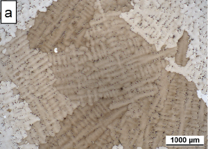
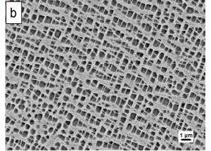
Figure 1: Microstructure of RENE 80 by using OM (a) and REM (b).

Cylindrical rods were eroded by electro-discharge-machining from the slabs and afterwards turned to the final specimen geometry. Figure 2 shows one of the specimen geometries used for the LCF tests. The diameter ($D_{\textrm{small}}$), the gauge length ($L_{\textrm{small}}$) and the resulting surface and volume of the gauge section of the specimen are listed in Table 2.

$L_{\textrm{small}}$ [mm]	$D_{\textrm{small}}$ [mm]	Surface $\textrm{[mm}^{2}\textrm{]}$	Vol. $\textrm{[mm}^{3}\textrm{]}$
12.0	7.0	263.9	461.8

Table 2: Geometrical parameters of the small specimen geometry.

In addition to tests with this specimen geometry, we consider already existing LCF test results of Siemens AG for T=850$\,{}^{\circ}$C regarding the same material subject to the same heat treatment. The corresponding specimen geometry has a 2.86 times larger surface of the gauge section. In the following, we refer to these specimens as the standard specimens and to the specimens according to Table 2 as the small ones.

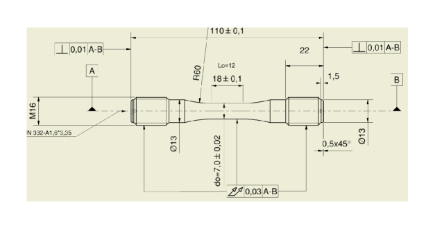
Figure 2: Small specimen geometry for the fatigue tests.

For the investigation of the LCF lifetime behavior a servo-hydraulic fatigue testing machine with a maximum load of 100kN has been used. All LCF tests were carried out at $850\,^{\circ}$C at isothermal conditions in total strain control with a load ratio of $R=-1$. The load cycles were applied with triangular waveform at a frequency of 0.1Hz for high strain amplitudes ($\varepsilon_{a,\textrm{tot}}=0.55\%-0.65\%$) and $1$Hz for low strain amplitudes ($\varepsilon_{a,\textrm{tot}}=0.15\%-0.25\%$), respectively.

The crack-initiation lifetime is defined by a drop of the curve which is given by the maximum stress’ dependence on the number of already conducted load cycles. In case of no extremely large strain amplitude, this curve starts with approximately stable maximum stress before first crack initiations take place after a certain number of load cycles. When the first crack initiation occurs, the curve starts to drop as the cross-section area of the specimen decreases and thereby a lower tensile force is needed for imposing the prescribed strain amplitude. Note that the maximum stress is defined as the ratio of this tensile force (which depends on the current load cycle) and the fixed cross-section area of the specimen at the beginning of the LCF tests. Considering equal crack areas at crack initiation life $N_{i}$, the drop of the maximum stress was calculated separately for each geometry using the following equation:

$$S_{\textrm{small}}=S_{\textrm{standard}}\cdot\left(\frac{D_{\textrm{standard}}}{D_{\textrm{small}}}\right)^{2}$$ (22)

with $S_{\textrm{small/standard}}$ stress drops and $D_{\textrm{small/standard}}$ diameters of the small and standard specimen, respectively. The LCF test results for both specimen geometries are given in Figure 3 in the representation total strain amplitude ($\varepsilon_{a,\textrm{tot}}$) versus cycles to crack initiation ($N_{i}$).

3.2 Calibration of the Model and Prediction of Wöhler Curves

For the calibration of the model we have chosen the LCF test results $N_{i_{\textrm{standard}}}(\varepsilon_{a,\textrm{tot}})$ of the standard specimen geometry as the corresponding data basis is much larger here than for the small specimen. In Figure 3, test results for both geometries are shown, together with several Wöhler curves.

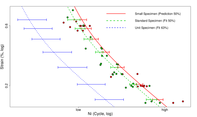
Figure 3: LCF test results of the small (red) and standard (green) specimens. The standard specimen data are used for the calibration of the model. The calibration leads to the Wöhler curve (blue) of the unit specimen and, via formulae (19), to the Wöhler curve (green) of the standard specimen. The Wöhler curve (red) for the small specimen is predicted by the probabilistic model for LCF, where formulae (19) is employed, again.

The calibration of the probabilistic model for LCF is conducted according to the maximum likelihood method as described at the end of Subsection 2.2. The Wöhler curve of the unit (blue) specimen describes the functional dependence of the Weibull scale parameter on the strain amplitude $\varepsilon_{a,\textrm{tot}}$. Using formulae (19) leads to the Wöhler curves of the standard (green) and small (red) specimens with the 50$\%$-Weibull quantiles (medians). It is important to point out that the curves for the unit and standard specimens are based on the calibration, whereas the curve for the small specimen is a pure prediction of our probabilistic model. The horizontal bars denote the 92.5$\%$ confidence intervals – see Figure 3 – that have been computed via a fully parametric bootstrap sampling procedure in conjunction with the percentile method as described in [7, 14].

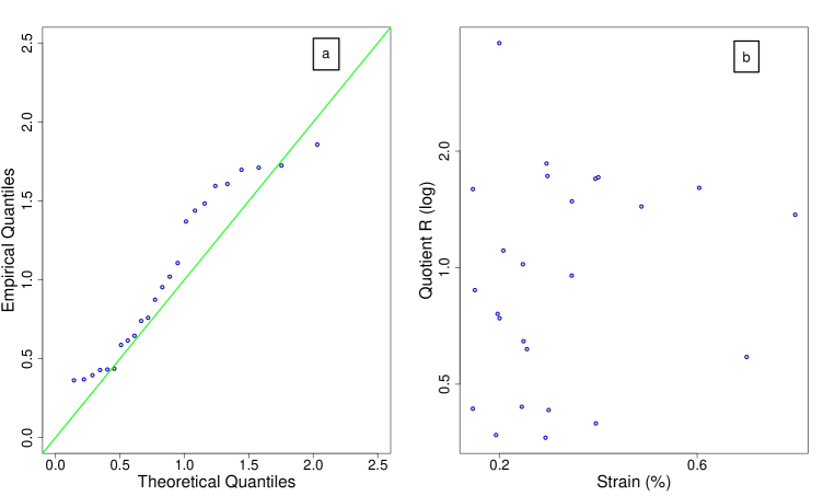
Figure 4: Q-Q plot (a) with respect to a Weibull fit of quotient $q$ with scale $1$ and values of $q$ (b) at the tested strain amplitudes of the standard specimen.

For model diagnostics we consider the quotient

$$q=\frac{N_{i_{\textrm{standard}}}(\varepsilon_{a,\textrm{tot}})}{N_{i_{\textrm{det,standard}}}(\varepsilon_{a,\textrm{tot}})},$$ (23)

with $N_{i_{\textrm{standard}}}(\varepsilon_{a,\textrm{tot}})$ the actual test results of the standard specimens and $N_{i_{\textrm{det,standard}}}(\varepsilon_{a,\textrm{tot}})$ the corresponding fit of our model for the Weibull scale parameter. Figure 4 (a) shows a Q-Q plot with respect to a Weibull fit of $q$ with scale $1$. According to the Kolmogorov - Smirnov test with a p-value of 17$\%$, deviations from the Weibull distribution are not statistically significant which supports the Weibull approach (10) of our model. Recalling our assumption that the shape parameter $m$ does not depend on the strain state $\varepsilon$, we consider Figure 4 (b) which shows the values of $q$ at the tested strain levels of the standard specimen. Statistical tests cannot exclude a deterministic relationship between $q$ and $\varepsilon_{a,\textrm{tot}}$, in particular for higher strain ranges, which could be finally assessed with additional test results. Nevertheless, note that the assumption of no significantly deterministic relationship between those quantities is often used, in particular with respect to design relevant strain ranges.

Because the unit specimen has the largest gauge surface of all considered specimens its Wöhler curve is expected to contain the lowest life-cycle numbers $N_{i}$. This expectation is confirmed by the results shown in Figure 3. The figure also shows that the fitting procedure and formulae (19) are able to yield an appropriate Wöhler curve for the standard specimen. The predicted Wöhler curve for the small specimen is shifted to higher life-cycle numbers $N_{i}$ due to the incorporated size effect in our model. However, this predicted shift is not very large so that statements on the position of the curves compared to the test results have to be considered carefully. Nevertheless, the LCF test results support the assumption of a size effect for lower strain amplitudes. A size effect is more difficult to be recognized in the range of higher strain amplitudes, where plasticity effects are present. Comparing the position of the Wöhler curve and the LCF test results of the small specimen shows that our model estimates the size effect for lower strain amplitudes very well. In the range of higher strain amplitudes, where plasticity comes into play, our model seems to overestimate the shift to higher life-cycle numbers $N_{i}$. Note that the prediction of our model in that range has to be judged more carefully as only few calibration data were available in the plastic range. This is also affirmed by the confidence intervals which overlap more significantly in the plastic range. Moreover, consider the large scatter in the data and a variety of possible error sources in the experiments such as determining crack initiation, stress and strain amplitudes and slight deviations from the homogeneity of strain and temperature fields.

Further investigations on the size effect can be found in [8, 15, 16], where a smaller size effect for higher strain amplitudes is stated as well. According to [15, 16] the small difference in the size effect between high and low strain amplitudes may be explained by the fact that at lower strain amplitudes plastic deformation is concentrated in individual slip systems of favorably orientated grains, whereas at higher strain amplitudes plastic deformation takes place over the whole gauge length. According to [17] this results in an increased number of activated slip bands, so that a possible effect of surface grain orientation becomes less important.

4 Conclusions

A probabilistic model for LCF has been derived from concepts of fatigue analysis and point processes. It was shown that this model leads to a new interpretation of the CMB parameters which are independent of the geometry of standardized test specimens. Moreover, we have derived formulae for the prediction of Wöhler curves of standardized specimens with different surface areas. The prediction of such Wöhler curves was also the basis for the validation of our probabilistic approach.

The calibration of our model resulted in an appropriate fit for the Wöhler curve of the standard specimen. For strain amplitudes not too high, we could find a size effect regarding the test results of the small specimen, and our model was able to appropriately predict the size effect’s impact on the Wöhler curve. But for higher strain amplitudes in the plastic range, the size effect could not be confirmed without ambiguity. In this range our model seems to overestimate a size effect. However, considering the large scatter for LCF life and a variety of possible error sources regarding the LCF tests, this overestimation could not be finally concluded.

For future work, we propose to analyze the size effect in the plastic range in more detail. Recall that for larger values of $m$, i.e. for smaller scatter, the size effect decreases. More LCF test results in the plastic range could lead to a different value of $m$. Furthermore, one could change the Weibull hazard approach according to another distribution such as log-normal distribution. Furthermore, it might be worthwhile to incorporate a mathematical concept for the slip systems of the grains which could lead to a smaller scatter of the corresponding LCF results as the random behavior of the slip systems is then taken into account.

The comparison of predicted Wöhler curves for notched specimens with corresponding LCF test results will play an important role in future work because this will show how effective the proposed model will be in case of inhomogeneous strain fields. It then might turn out that the model needs to incorporate local information on the strain gradient. Similarly, the aspect of inhomogeneous temperature fields can be taken into account in the model if the CMB approach considers an appropriate deterministic temperature model for LCF. The model can also consider volume integrals and can thereby be applied to volume driven LCF failure mechanism with initial creep damage and to HCF failure mechanism, for example.

The model is also intended to be applied to FEA simulations of engineering parts under cyclic loading. These simulations in conjunction with field data can be employed to validate or recalibrate the proposed model. Finally, let us mention an improved link to shape optimization which is given by our probabilistic model. Due to the probabilistic nature of our model the new objective functional (11) for LCF life is sufficiently regular so that efficient gradient based shape optimization schemes can be conducted, confer [18, 19].

References

- [1] M. Bäker, H. Harders and J. Rösler, Mechanisches Verhalten der Werkstoffe, third edition, Vieweg+Teubner, Wiesbaden, 2008.
- [2] B. Fedelich, A Stochastic Theory for the Problem of Multiple Surface Crack Coalescence, International Journal of Fracture 91 (1998) 23- 45.
- [3] D. Sornette, T. Magnin and Y. Brechet, The Physical Origin of the Coffin-Manson Law in Low-Cycle Fatigue, Europhys. Lett. 20 (5) (1992) 433-438.
- [4] M. Sherman, Spatial Statistics and Spatio-Temporal Data: Covariance Functions and Directional Properties, Wiley Series in Probability and Statistics, 2010.
- [5] O. Kallenberg, Random Measures, third edition, Akademie Verlag, Berlin, 1983.
- [6] A. Baddeley, P. Gregori, J. Mateu, R. Stoica and D. Stoyan, editors, Case Studies in Spatial Point Process Modeling, Lecture Notes in Statistics, 185, Springer, 2006.
- [7] L. A. Escobar and W. Q. Meeker, Statistical Methods for Reliability Data, Wiley-Interscience Publication, New York, 1998.
- [8] D. Radaj and M. Vormwald, Ermüdungsfestigkeit, third edition, Springer, Berlin Heidelberg, 2007.
- [9] G. Schott, Werkstoffermüdung - Ermüdungsfestigkeit, Deutscher Verlag für Grundstoffindustrie, fourth edition, Stuttgart, 1997.
- [10] A. Ern and J.-L. Guermond, Theory and Practice of Finite Elements, Springer, New York, 2004.
- [11] P. Ciarlet, Basic Error Estimates for Elliptic Problems, Vol. II: Finite Element Methods, ch. 2. Handbook of Numerical Analysis, North-Holland, Amsterdam, 1991.
- [12] K. H. Kloos, A. Buch and D. Zankov, Pure Geometrical Size Effect in Fatigue Tests with Constant Stress Amplitude and in Programme Tests Journal of Materials Technology 12 (1981) 40-50.
- [13] I. Bazios and H.-J. Gudladt, Die Anrisslebensdauerabschätzung unter Berücksichtigung des Statistischen Größeneinflusses am Beispiel der AlMgSi0,7-Legierung, Materialwissenschaften und Werkstofftechnik 35 (2004) 21-28.
- [14] A. C. Davison and D. V. Hinkley, Bootstrap Methods and their Application, Camebridge University Press, New York, 1997.
- [15] V. P. Bennett and D.L. McDowell, Polycrystal Orientation Distribution Effects on Microslip in High-Cycle Fatigue, International Journal of Fatigue 25 (2003) 27-39.
- [16] F. P. E. Dunne and A. Manonukul, High and Low-Cycle Fatigue Crack Initiation using Polycrystal Plasticity, Proc. Roy. Soc. Lond. A 460 (2004) 1881-1902.
- [17] Y. Duyi , P. Dehai, W. Zhenlin, X. Haohao, M. Xiaoyu, X. Changwei, C. Xiaolin, Low-Cycle Fatigue Behavior of Nickel-Based Superalloy GH4145/SQ at Elevated Temperature, Materials Science and Engineering A 373 (2004) 54-64.
- [18] J. Sokolowski and J.-P. Zolesio, Introduction to Shape Optimization - Shape Sensivity Analysis, Springer, Berlin Heidelberg, 1992.
- [19] J. Haslinger and R. A. E. Mäkinen, Introduction to Shape Optimization - Theory, Approximation and Computation, SIAM - Advances in Design and Control, 2003.