Global cosmological dynamics for the scalar field representation of the modified Chaplygin gas

Abstract

In this paper we investigate the global dynamics for the minimally coupled scalar field representation of the modified Chaplygin gas in the context of flat Friedmann-Lemaître-Robertson-Walker cosmology. The tool for doing this is a new set of bounded variables that lead to a regular dynamical system. It is shown that the exact modified Chaplygin gas perfect fluid solution appears as a straight line in the associated phase plane. It is also shown that no other solutions stay close to this solution during their entire temporal evolution, but that there exists an open subset of solutions that stay arbitrarily close during an intermediate time interval, and into the future in the case the scalar field potential exhibits a global minimum.

PACS numbers: 04.20.-q, 98.80.-k, 98.80.Bp, 98.80.Jk

1 Introduction

The total matter content in the universe, now and in the distant past, is a mystery. As a consequence cosmological models abound, both as regards fields and the dynamical laws they obey. This is reflected in a plethora of inflationary models and models for dark matter and energy, in the context of general relativity and in modified gravity theories. This entails possibilities for new physical insights, but it also causes explanatory problems; the latter exemplified by e.g. fine-tuning problems of potentials (see e.g. [1]) and initial data.

One attempt to fit theory with observations is to phenomenologically match the observed expansion history by imposing conditions on e.g. the time development of the cosmological scale factor, or by imposing a relationship between pressure and energy density, and then use such a relationship to produce a field description, as discussed in e.g. [2]–[4] and references therein. The arguably simplest field theoretic description is a minimally coupled scalar field within the context of flat Friedmann-Lemaître-Robertson-Walker (FLRW) cosmology, see e.g. [5]–[8], and references therein. A field theoretic description, however, leads to that the original relationship only is obeyed by particular solutions to the field problem it has generated, as pointed out in e.g. [9]–[11]. This is due to that a field theoretic description adds degrees of freedom, e.g. a single minimally coupled scalar field adds one degree of freedom to a perfect fluid description with a barotropic equation of state. This then leads to the issue how the global solution space of the field theoretic description is related to that of the generating relationship.

Although some work on the issue of initial data not corresponding to the generating conditions has been done, as exemplified by the numerical examples in [10] and the investigation in [11] for the Chaplygin gas, as far as the author knows there seems to be no global dynamical systems investigations of this issue. In this paper, which is the first in a series that will address fine-tuning problems with global dynamical systems methods, we will, as a specific example, consider flat FLRW cosmology and the minimally coupled scalar field description of the modified Chaplygin gas. The modified Chaplygin gas is characterized by an equation of state (see e.g. [12]–[14])

$$p=(\gamma-1)\rho-M\rho^{-\mu},$$ (1)

where $p$ is the pressure of the fluid, $\rho$ its energy density and $M$, $\mu$ and $\gamma$ are free parameters. For simplicity, we will here restrict their range to $M>0$, $\mu>0$, $1\leq\gamma<2$. The value $\gamma=1$ leads to the so-called generalized Chaplygin gas while $\gamma=\mu=1$ corresponds to the original Chaplygin gas. This equation of state can be used to construct the scalar field potential for a scalar field $\phi$, see e.g. [15, 16, 12, 13], which can be written as

$$V=\frac{V_{0}}{2}\left[(2-\gamma)\cosh^{\frac{2}{1+\mu}}\tilde{\phi}+\gamma\cosh^{\frac{-2\mu}{1+\mu}}\tilde{\phi}\right]=\frac{V_{0}}{2}\cosh^{\frac{2}{1+\mu}}\tilde{\phi}\left[2-\gamma\tanh^{2}\tilde{\phi}\right],$$ (2)

where $V_{0}:=(M/\gamma)^{\frac{1}{1+\mu}}$, $\tilde{\phi}:=\frac{1}{2}(1+\mu)\sqrt{3\gamma}(\phi-\phi_{0})$.

In this paper we will introduce new bounded variables that in the flat FLRW case with the above minimally coupled scalar field lead to a 2-dimensional regularized dynamical system, with $\mu$ and $\gamma$ as parameters. This will yield a global picture of the scalar field dynamics, and provide a context for the generating modified Chaplygin gas perfect fluid solution, which, for a given $\mu$ and $\gamma$, appears as a straight line in our regularized 2-dimensional dynamical system. Moreover, the scalar field potential (2) yields three classes of different behavior, characterized by conditions on $\mu$ and $\gamma$ associated with a bifurcation for the dynamical system; notably the original Chaplygin gas appears as a member of the class of models associated with the bifurcation.

The outline of the paper is as follows. In the next section we derive, in a step by step manner, our regularized dynamical system on a bounded state space, where the boundaries are included. In section 3 we perform a both local and global dynamical systems analysis which leads to a complete understanding of the solution space. In particular the generating perfect fluid is identified as an invariant subset corresponding to a straight line in the phase plane, and this subset is subsequently contextualized by the local and global phase plane results. The paper is concluded with a discussion in section 4.

2 Dynamical systems formulation

The field equations for a minimally coupled scalar field $\phi(t)$ with potential $V(\phi)$ for flat FLRW cosmology are given by

$$3H^{2} ={\textstyle{1\over 2}}\dot{\phi}^{2}+V=:\rho_{\phi},$$ (3a)

$$\dot{H} =-H^{2}-{\textstyle{1\over 3}}(\dot{\phi}^{2}-V)=-{\textstyle{1\over 2}}\dot{\phi}^{2},$$ (3b)

$$0 =\ddot{\phi}+3H\dot{\phi}+V_{\phi}.$$ (3c)

Here an overdot signifies the synchronous time, $t$, derivative; $V_{\phi}:=dV/d\phi$, and where we have used units to set $c=1=8\pi G$, where $c$ is the speed of light and $G$ is the gravitational constant. The Hubble variable $H$ is given by $H=\dot{a}/a$, where $a(t)$ is the cosmological scale factor; throughout we will assume an expanding Universe, i.e. $H>0$. It follows from (3b) that the deceleration parameter, $q$, which is defined via $\dot{H}=-(1+q)H^{2}$, is given by

$$q=-1+\frac{1}{2}\left(\frac{\dot{\phi}}{H}\right)^{2}.$$ (4)

A commonly used formulation when $V\geq 0$ is obtained by ‘Hubble-normalization’ which is used extensively in cosmology (see e.g. [3, 17] for FLRW scalar field cosmology, and e.g. [17, 18] for anisotropic spatially homogeneous cosmology):

$$x:=\frac{\dot{\phi}}{\sqrt{6}\,H}\qquad y:=\frac{\sqrt{V}}{\sqrt{3}\,H},$$ (5)

and a new time variable ${\tau}$, defined by $dt=H^{-1}d{\tau}$, which means that ${\tau}=\ln(a/a_{0})$ ($a_{0}=a(t_{0})$, where $t_{0}$ is some convenient reference time), where $\tau$ sometimes is referred to as $N$, the number of e-folds from the reference time $t_{0}$. This leads to:

$$x^{\prime} =-(3x-\sqrt{{\textstyle{3\over 2}}}\,\lambda)(1-x^{2}),$$ (6a)

$$y^{\prime} =(3x-\sqrt{{\textstyle{3\over 2}}}\,\lambda)xy,$$ (6b)

$$1 =x^{2}+y^{2},$$ (6c)

where a ^′ denotes differentiation with respect to ${\tau}$. The quantity $\lambda$ is defined by

$$\lambda=-\frac{V_{\phi}}{V},$$ (7)

and is a function of $\phi$ except when $V=c_{1}^{2}\exp(c_{2}\phi)$, where $c_{1}$ and $c_{2}$ are constants, since then $\lambda=-c_{2}$, which leads to a 1-dimensional problem for $x$. In general, since $\lambda=\lambda(\phi)$, one has to add the equation

$$\phi^{\prime}=\sqrt{6}x$$ (8)

to the system (6) to obtain a closed constrained system. In the above equations, the variable $y$ can be replaced by a variable $\Omega_{V}=y^{2}=1-x^{2}$ which can be globally solved for to yield a 2-dimensional unconstrained system for $x$ and $\phi$:

$$x^{\prime} =-(3x-\sqrt{{\textstyle{3\over 2}}}\,\lambda)(1-x^{2}),$$ (9a)

$$\phi^{\prime} =\sqrt{6}\,x.$$ (9b)

Although $x$ is bounded, $\phi$ is not. Furthermore, $\lambda(\phi)$ need not be bounded either. In the special case that $\lambda(\phi)$ is bounded for all $\phi$, one can introduce a new variable $Y(\phi)$ to obtain a new system

$$x^{\prime} =-(3x-\sqrt{{\textstyle{3\over 2}}}\,\lambda)(1-x^{2}),$$ (10a)

$$Y^{\prime} =\sqrt{6}\,\frac{dY}{d\phi}\,x,$$ (10b)

where, with some abuse of notation $\lambda=\lambda(Y)$ and $\frac{dY}{d\phi}=\frac{dY}{d\phi}(Y)$. It turns out that it is possible to choose a bounded variable $Y$ for a number of scalar field potentials so that the equations (10) become regular on a relatively compact state space, whose boundary can be included in the dynamical systems analysis, which allows one to obtain a global picture of the dynamics.

It follows from (5), (6c) and (10) that the variable $x\in(-1,1)$ can be extended to include the boundaries $x=\pm 1$ so that $x\in[-1,1]$. The invariant boundary subsets $x=\pm 1$, correspond to $y=0=V$, and are hence associated with the massless scalar field problem, and we will therefore refer to them as the massless scalar field boundary subsets, and denote them by ${\cal M_{\pm}}$. Note that

$$w:=\frac{p_{\phi}}{\rho_{\phi}}=\frac{{\textstyle{1\over 2}}\dot{\phi}^{2}-V(\phi)}{{\textstyle{1\over 2}}\dot{\phi}^{2}+V(\phi)}=2x^{2}-1,\qquad q=-1+3x^{2},$$ (11)

and that acceleration ($q<0$) hence occurs if $x^{2}<\frac{1}{3}$, which corresponds to $w<-\frac{1}{3}$, while $q=2$, $w=1$ on ${\cal M_{\pm}}$. Furthermore, it follows from (3a) and (5) that

$$3H^{2}=\frac{V(Y)}{1-x^{2}}=:Z(Y,x),$$ (12)

while (3b) gives

$$Z^{\prime}=-6x^{2}\,Z,$$ (13)

and hence $Z$ is monotonically decreasing towards the future, except when $x=0$ belongs to an invariant subset. Next we turn to our dynamical systems formulation of the modified Chaplygin gas scalar field problem.

Recall that the scalar field potential associated with the modified Chaplygin gas given in (2) could be written as

$$V=\frac{V_{0}}{2}\cosh^{\frac{2}{1+\mu}}\tilde{\phi}\left[2-\gamma\tanh^{2}\tilde{\phi}\right].$$ (14)

This potential is invariant under the change $\tilde{\phi}\rightarrow-\tilde{\phi}$, which will give rise to a discrete symmetry in the dynamical systems treatment. It is instructive to Taylor expand the potential at $\tilde{\phi}=0$:

$$V=V_{0}\!\left[1+\beta\tilde{\phi}{}^{2}+{\textstyle{1\over 8}}\left((2-\gamma)\gamma+4\beta(\beta-{\textstyle{1\over 3}})\right)\!\tilde{\phi}{}^{4}+\dots\right],$$ (15a)

where

$$\beta:=\frac{1}{1+\mu}-\frac{\gamma}{2}=\frac{2-\gamma(1+\mu)}{2(1+\mu)}.$$ (15b)

The potential has a global minimum at $\tilde{\phi}=0$ if $\beta\geq 0$, although the minimum is quite ‘flat’ if $\beta=0$ since then $d^{2}V/d\tilde{\phi}{}^{2}|_{\tilde{\phi}=0}=0$, while $\tilde{\phi}=0$ is local maximum surrounded by two identical minima if $\beta<0$; see Figure 1. As can be expected, this will lead to a bifurcation at $\beta=0$ in the dynamical systems analysis below.

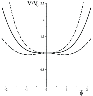
Figure 1: Representatives of the three types of potentials characterized by $\beta>0$, with $\gamma=\frac{4}{3},\,\mu=\frac{1}{4}$ (dashed dotted line); $\beta=0$, with $\gamma=1=\mu$ (solid line); $\beta<0$, with $\gamma=1,\,\mu=2$ (dashed line), where $\beta=\frac{1}{1+\mu}-\frac{\gamma}{2}$.

To obtain a regular dynamical system on a relatively compact state space we introduce the variable

$$Y:=\tanh\tilde{\phi},$$ (16)

which leads to that

$$x^{\prime} =-(3x-\sqrt{{\textstyle{3\over 2}}}\,\lambda)(1-x^{2}),$$ (17a)

$$Y^{\prime} ={\textstyle{3\over 2}}(1+\mu)\sqrt{2\gamma}(1-Y^{2})x,$$ (17b)

where

$$\lambda=-\sqrt{3\gamma}\,Y\left(\frac{2-\gamma-\gamma\mu(1-Y^{2})}{2-\gamma Y^{2}}\right),$$ (17c)

Since $\lambda(Y)$ is a differentiable function for $Y\in[-1,1]$, we can extend the state space to not just including the boundaries $x^{2}=1$ but also $Y^{2}=1$. This leads to a state space ${\bf S}$ for which $x\in(-1,1)$, $Y\in(-1,1)$, which when extended to include its boundary yields $\bar{\bf S}$: $x\in[-1,1]$, $Y\in[-1,1]$. In addition to the massless scalar field boundary subsets ${\cal M}_{\pm}$, we therefore also have the invariant boundary subsets $Y=\pm 1$, for which $\lambda(Y=1)=-\lambda(Y=-1)$ is a constant, and hence the equation for $x$ is the same as that for a single exponential field potential with $V=c_{1}^{2}\exp(-\lambda(Y=\pm 1))$. We will therefore refer to the invariant $Y=\pm 1$ boundary subsets as the exponential term subsets, and will denote them by ${\cal E}_{\pm}$. Furthermore, the system (17) on $\bar{\bf S}$ admits a discrete symmetry; it is invariant under the transformation $(x,Y)\rightarrow-(x,Y)$, a property that is a consequence of the discrete symmetry of the potential $V$.

In addition to the boundary subsets, the system (17) admits another identifiable 1-dimensional subset, namely the interior subset that is associated with the perfect fluid solution that generated the scalar field potential. This subset can conveniently be found by using that $w=2x^{2}-1$ in general and that $w=w(\phi(Y))$ for the perfect fluid solution, where $w(\phi(Y))$ is obtained easily from the expressions in e.g. [12, 13]. By identifying the two expressions for $w$, it then follows straightforwardly that the perfect fluid solution satisfies

$$(\sqrt{2}\,x+\sqrt{\gamma}\,Y)(\sqrt{2}\,x-\sqrt{\gamma}\,Y)=0,$$ (18)

and therefore one of these factors must be zero. Taking the combination $\sqrt{2}\,x^{\prime}+\sqrt{\gamma}\,Y^{\prime}$ gives

$$(\sqrt{2}\,x+\sqrt{\gamma}\,Y)^{\prime}=\frac{3}{2}\!\left(\sqrt{2}\,x+\sqrt{\gamma}\,Y\right)\!\left(\sqrt{2}\,x(\sqrt{2}\,x-\sqrt{\gamma}\,Y)-\frac{(2-\sqrt{2\gamma}\,xY)R}{2-\gamma Y^{2}}\right),$$ (19)

where

$$R:=2-\gamma-\gamma\mu(1-Y^{2}),$$ (20)

and hence $\sqrt{2}\,x+\sqrt{\gamma}\,Y=0$ is an invariant subset (which, by inspection, $\sqrt{2}\,x-\sqrt{\gamma}\,Y=0$ turns out not to be) describing the perfect fluid solution, which, due to the discrete symmetry, is represented by two equivalent solution trajectories. We will refer to the invariant subset $\sqrt{2}x+\sqrt{\gamma}\,Y=0$ as the ‘perfect fluid subset’ and will denote it as ${\cal PF}$, and the two perfect fluid trajectories as ${\cal PF}_{\pm}$, where the sign refers to the sign of $Y$.

The system (17) admits a number of fixed points:

$$\mathrm{dS}_{0}:\quad(x,Y) =(0,0),$$ (21a)

$$\mathrm{dS}_{\pm}:\quad(x,Y) =(0,\pm Y_{0})\quad Y_{0}:=\sqrt{1-\frac{2-\gamma}{\gamma\mu}},\quad\text{if}\quad\mu>\frac{2-\gamma}{\gamma},$$ (21b)

$$\mathrm{M}_{x=\pm 1}^{Y=\epsilon}:\quad(x,Y) =(\pm 1,\epsilon),\quad\text{where}\quad\epsilon=1\quad\text{or}\quad\epsilon=-1,$$ (21c)

$$\mathrm{PF}_{\pm}:\quad(x,Y) =(\mp\sqrt{\gamma/2},\pm 1).$$ (21d)

The fixed points $\mathrm{dS}_{0}$ and $\mathrm{dS}_{\pm}$ correspond to $w=-1$ and therefore represent de Sitter states. Note that the fixed points $\mathrm{dS}_{\pm}$ only exist when $\mu>\frac{2-\gamma}{\gamma}$, i.e., when $\beta<0$, which corresponds to the situation when the scalar field potential $V$ has two minima. The four fixed points $\mathrm{M}_{x=\pm 1}^{Y=\epsilon}$ at the corners of the phase plane have $w=1$ and hence correspond to massless scalar field states. Finally, the $\mathrm{PF}_{\pm}$ fixed points are the origin ($\alpha$ limits) of the perfect fluid solution trajectories ${\cal PF}_{\pm}$. At these fixed points $w=\gamma-1$, which is the limit of the perfect fluid equation of state towards the initial singularity when $\rho\rightarrow\infty$.

The Chaplygin gas case play a historical special role and it is of interest to write down the equations explicitly for this case, including its fixed points. In this case $p=-M\rho^{-1}$, and hence $\gamma=\mu=1$, which leads to the scalar field potential [15]

$$V=\frac{V_{0}}{2}\cosh\tilde{\phi}\left[2-\tanh^{2}\tilde{\phi}\right]=\frac{V_{0}}{2}\left[\cosh\tilde{\phi}+\cosh^{-1}\tilde{\phi}\right],$$ (22)

where $\tilde{\phi}:=\sqrt{3}(\phi-\phi_{0})$. As a consequence

$$x^{\prime} =-(3x-\sqrt{{\textstyle{3\over 2}}}\,\lambda)(1-x^{2}),$$ (23a)

$$Y^{\prime} =3\sqrt{2}(1-Y^{2})\,x,$$ (23b)

$$\lambda =-\sqrt{3}\left(\frac{Y^{3}}{2-Y^{2}}\right).$$ (23c)

The ${\cal PF}$ subset is characterized by $\sqrt{2}x+Y=0$, while the seven fixed points the dynamical system (23) admits are given by

$$\mathrm{dS}_{0}:\quad(x,Y) =(0,0),$$ (24a)

$$\mathrm{M}_{x=\pm 1}^{Y=\epsilon}:\quad(x,Y) =(\pm 1,\epsilon),\quad\text{where }\quad\epsilon=1\quad\text{or}\quad\epsilon=-1,$$ (24b)

$$\mathrm{D}_{\pm}:\quad(x,Y) =(\mp 1/\sqrt{2},\pm 1).$$ (24c)

The fixed points $\mathrm{PF}_{\pm}$ have here been denoted by $\mathrm{D}_{\pm}$ since $w=0$ in this case, and thus $\mathrm{D}_{\pm}$ represents a ‘dust’ state.

3 Dynamical systems analysis

3.1 Local fixed point analysis

The eigenvalues of the various fixed points of (17) are given by

$$\mathrm{dS}_{0}: \quad-{\textstyle{3\over 2}}\left[2-\gamma(1+\mu)\right], -{\textstyle{3\over 2}}\gamma(1+\mu),$$ (25a)

$$\mathrm{dS}_{\pm}: \quad-{\textstyle{3\over 2}}\left[1\pm\sqrt{9-4\gamma(1+\mu)}\right], \text{if}\quad\mu>\frac{2-\gamma}{\gamma},$$ (25b)

$$\mathrm{M}_{x=\mp 1}^{Y=\pm 1}: \quad 3\sqrt{2\gamma}\,(1+\mu), 3(2-\sqrt{2\gamma}),$$ (25c)

$$\mathrm{M}_{x=\pm 1}^{Y=\pm 1}: \quad-3\sqrt{2\gamma}\,(1+\mu), 3(2+\sqrt{2\gamma}),$$ (25d)

$$\mathrm{PF}_{\pm}: \quad 3\gamma(1+\mu), -{\textstyle{3\over 2}}(2-\gamma).$$ (25e)

As expected there is a bifurcation associated with the $\mathrm{PF}_{\pm}$ fixed points when $\gamma=2$, since $\gamma=2$ leads to that the perfect fluid solution asymptotically towards the past behave like a stiff fluid, which is equivalent to a massless scalar field. As a consequence, the $\mathrm{PF}_{\pm}$ fixed points pass through the $\mathrm{M}_{x=\mp 1}^{Y=\pm 1}$ points at this value for $\gamma$, which leads to a bifurcation. For simplicity we have therefore assumed that $\gamma<2$, but we will return to the case $\gamma=2$ in the concluding discussion.

We also have a bifurcation at $2-\gamma(1+\mu)=0$ ($\beta=0$), which is when the $\mathrm{dS}_{\pm}$ fixed points merge with the $\mathrm{dS}_{0}$ fixed point. When $2-\gamma(1+\mu)<0$ ($\beta<0$) the fixed points $\mathrm{dS}_{\pm}$ exist and are hyperbolic sinks, while $\mathrm{dS}_{0}$ is a hyperbolic saddle. In this case only two solutions end at $\mathrm{dS}_{0}$ (has $\mathrm{dS}_{0}$ as their $\omega$ limit) and these are the perfect fluid trajectories ${\cal PF}_{\pm}$, since the invariant subset ${\cal PF}$ can be identified as the stable manifold of $\mathrm{dS}_{0}$. When $2-\gamma(1+\mu)>0$ ($\beta>0$) the fixed point $\mathrm{dS}_{0}$ becomes a hyperbolic sink, however, when $2-\gamma(1+\mu)=0$ $\mathrm{dS}_{0}$ is a non-hyperbolic sink (as will be shown below in the global analysis). Note that the Chaplygin case belongs to this case. The fixed points $\mathrm{M}_{x=\mp 1}^{Y=\pm 1}$ are hyperbolic sources while $\mathrm{M}_{x=\pm 1}^{Y=\pm 1}$ are hyperbolic saddles, with eigenvectors along the boundaries, so there are no solutions originating from these fixed points into ${\bf S}$. Finally, $\mathrm{PF}_{\pm}$ are hyperbolic saddles where each fixed point gives rise to a single solution entering the state space ${\bf S}$, the perfect fluid solution ${\cal PF}_{\pm}$ (thus being the unstable manifold of $\mathrm{PF}_{\pm}$).

3.2 Global dynamical systems analysis

It follows from (13) and that

$$V=V(Y)=\frac{V_{0}}{2}(1-Y^{2})^{-\frac{1}{1+\mu}}(2-\gamma Y^{2}),$$ (26)

that $\tilde{Z}:=(1-Y^{2})^{-\frac{1}{1+\mu}}(2-\gamma Y^{2})(1-x^{2})^{-1}>0$ on ${\bf S}$ satisfies $\tilde{Z}^{\prime}=-6x^{2}\,\tilde{Z}$ and hence that

$$\bar{Z}^{\prime}=-6x^{2}\,\bar{Z}(1-\bar{Z}),\qquad\bar{Z}:=\frac{\tilde{Z}}{1+\tilde{Z}}=\frac{2-\gamma Y^{2}}{(1-Y^{2})^{\frac{1}{1+\mu}}(1-x^{2})+2-\gamma Y^{2}}.$$ (27)

Thus $\bar{Z}$ is a bounded monotone decreasing function on ${\bf S}\cap\mathrm{dS}_{0}$ when $2-\gamma(1+\mu)\geq 0$ ($\beta\geq 0$) and on ${\bf S}\cap\mathrm{dS}_{0}\cap\mathrm{dS}_{+}\cap\mathrm{dS}_{-}$ when $2-\gamma(1+\mu)<0$ ($\beta<0$), since the fixed points are the only invariant subsets on $x=0$.

As a consequence, when $2-\gamma(1+\mu)\geq 0$, i.e., when $\beta\geq 0$, all solutions in ${\bf S}$, except for the fixed point $\mathrm{dS}_{0}$, originate from the boundary $\partial{\bf S}$ where $\bar{Z}$ has its maximum $\bar{Z}=1$. It also follows that when $\beta<0$ all solutions also originate from the boundary $\partial{\bf S}$, except for the fixed points $\mathrm{dS}_{*}$ and the two solutions that originate from $\mathrm{dS}_{0}$. Combining this with the structure on the boundary, and the hyperbolic eigenvalues of the fixed points on $\partial{\bf S}$, it follows that when $\beta\geq 0$ all orbits in ${\bf S}$ originate from the sources $\mathrm{M}_{x=\mp 1}^{Y=\pm 1}$ except for the two perfect fluid trajectories ${\cal PF}_{\pm}$ which originate from $\mathrm{PF}_{\pm}$. Furthermore, the monotone function obtains its minimum $\bar{Z}=\frac{2}{3}$ at $\mathrm{dS}_{0}$ which is the future attractor for all orbits in ${\bf S}$, i.e., they all have $\mathrm{dS}_{0}$ as their $\omega$ limit (i.e., $\mathrm{dS}_{0}$ is a global sink on ${\bf S}$, even though it is a non-hyperbolic fixed point when $\beta=0$). Note that this is the case the Chaplygin gas belongs to. On the other hand, when $\beta<0$ all solutions end at the hyperbolic sinks $\mathrm{dS}_{\pm}$ except for the perfect fluid trajectories ${\cal PF}_{\pm}$, which end at $\mathrm{dS}_{0}$, as mentioned above. Note also that the unstable manifold of $\mathrm{dS}_{0}$ yields two solution trajectories that end at $\mathrm{dS}_{\pm}$, respectively, which follows from the monotone function in combination with that $\mathrm{dS}_{0}$ is a hyperbolic saddle in this case. These results are illustrated by the phase plane portraits given in Figure 2.

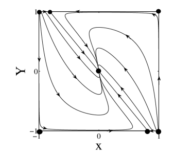
(a) $\gamma=\frac{4}{3},\,\mu=\frac{1}{4}$.

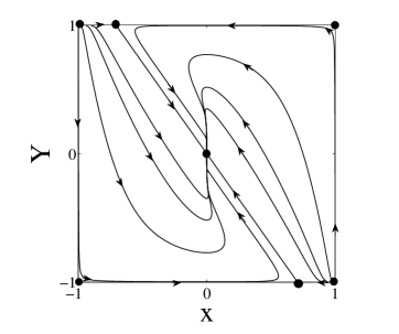
(b) $\gamma=1,\,\mu=1$.

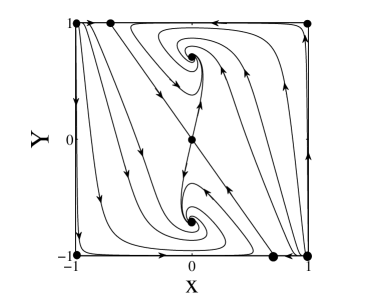
(c) $\gamma=1,\,\mu=2$.

Figure 2: Representative phase planes for the three cases characterized by $\beta>0$ ($\gamma=\frac{4}{3},\,\mu=\frac{1}{4}$), $\beta=0$ ($\gamma=1,\,\mu=1$) and $\beta<0$ ($\gamma=1,\,\mu=2$), where $\beta=\frac{1}{1+\mu}-\frac{\gamma}{2}$.

Remark.

The present statements concerning the use of the monotone function can be formalized by means of the Monotonicity Principle [18], which is stated as follows: Let $\phi_{t}$ be a flow on $\mathbb{R}^{n}$ with $S$ an invariant set. Let $Z:S\rightarrow\mathbb{R}$ be a $C^{1}$ function whose range is the interval $(a,b)$ where $a<b$. If $Z$ is decreasing on orbits in $S$, then for all ${\bf x}\in S$ the $\omega$ and $\alpha$ limits belong to the boundary of $S$ according to

$$\omega({\bf x})\subseteq\{{\bf s}\in\bar{S}\!\setminus\!S|\lim_{{\bf y}\rightarrow{\bf s}}Z({\bf y})\neq b\},$$

$$\alpha({\bf x})\subseteq\{{\bf s}\in\bar{S}\!\setminus\!S|\lim_{{\bf y}\rightarrow{\bf s}}Z({\bf y})\neq a\}.$$

The existence of a monotone function on $S$ therefore e.g. excludes any periodic orbits in $S$.

4 Discussion

We have here shown that the perfect fluid solution that generates the scalar field problem of the modified Chaplygin case appears as two straight lines in the phase plane. Moreover, the two straight lines originate from fixed points that correspond to the scale invariant perfect fluid solution with a linear equation of state $p=(\gamma-1)\rho$ on 1-dimensional boundaries that describe the scalar field problem corresponding to an exponential potential, which this scale-invariant solution generates. All other scalar field solutions originate from fixed points that correspond to scale-invariant massless scalar field solutions (except for the two solution that originate from the de Sitter fixed point $\mathrm{dS}_{0}$ and ending at the de Sitter fixed points $\mathrm{dS}_{\pm}$ when $\beta<0$). Hence no other solutions behave like the perfect fluid solutions towards the past limit (which perhaps is a somewhat mote issue in the present context since the purpose of these particular models is to describe intermediate and late stage behavior).

The role of the perfect fluid solution in the scalar field case for the Chaplygin gas has been previously discussed in [10] and [11] and hence the role of the perfect fluid solution in the case $\beta\geq 0$ deserves some comments ($\beta\geq 0$ is assumed throughout the subsequent discussion). Let us first give the linearization of ${\cal PF}$:

$$(\sqrt{2}\,x+\sqrt{\gamma}\,Y)^{-1}(\sqrt{2}\,x+\sqrt{\gamma}\,Y)^{\prime}|_{x=-\sqrt{\gamma/2}\,Y} =\frac{3}{2}\left[2\gamma\,Y^{2}-R\left(\frac{2+\gamma\,Y^{2}}{2-\gamma\,Y^{2}}\right)\right],$$ (28a)

$$(\sqrt{2}\,x+\sqrt{\gamma}\,Y)^{-1}(\sqrt{2}\,x+\sqrt{\gamma}\,Y)^{\prime}|_{\mathrm{PF}_{\pm}} =-{\textstyle{3\over 2}}(2-\gamma),$$ (28b)

$$(\sqrt{2}\,x+\sqrt{\gamma}\,Y)^{-1}(\sqrt{2}\,x+\sqrt{\gamma}\,Y)^{\prime}|_{\mathrm{dS}_{0}} =-{\textstyle{3\over 2}}\left[2-\gamma(1+\mu)\right],$$ (28c)

where $R=2-\gamma-\gamma\mu(1-Y^{2})$. Here the values at the fixed points $\mathrm{PF}_{\pm}$ and ${\mathrm{dS}_{0}}$ are just one of the eigenvalues at each fixed point and show that the perfect fluid submanifold ${\cal PF}$ is stable at $\mathrm{PF}_{\pm}$ and at $\mathrm{dS}_{0}$ when $\beta>0$. Note, however, that the sign of the right hand side of (28a) depends on the value of $Y^{2}$ (and the values of $\mu$ and $\gamma$), as illustrated by the Chaplygin case $(\sqrt{2}\,x+Y)^{-1}(\sqrt{2}\,x+Y)^{\prime}|_{x=-\sqrt{1/2}\,Y}=\frac{3}{2}\,\frac{Y^{2}(3Y^{2}-2)}{2-Y^{2}}$. As a consequence, solutions nearby $\mathrm{PF}_{\pm}$ drift away slightly from ${\cal PF}_{\pm}$ during part of their intermediate evolution, as seen in Figure 2. This means that the perfect fluid submanifold ${\cal PF}$ is not stable everywhere, which is a physical effect that can be measured in terms of $x$ and hence the deceleration parameter $q$. Nevertheless, thanks to that $\mathrm{dS}_{0}$ is a sink, even in the $\beta=0$ case, solutions that are close to the fixed points $\mathrm{PF}_{\pm}$ stay close to the trajectories ${\cal PF}_{\pm}$ throughout their subsequent evolution. Indeed, there is an open set of solutions that are arbitrarily close to the perfect fluid solution throughout their intermediate and late time evolution when $\beta\geq 0$, which can be seen as follows.

Consider the two finite heteroclinic chains that start from the source $\mathrm{M}_{x=-1}^{Y=1}$ along the boundary $\partial{\bf S}$ that are described by

$$\mathrm{M}_{x=-1}^{Y=1} \longrightarrow\mathrm{PF}_{+}\longrightarrow\mathrm{dS}_{0},$$ (29a)

$$\mathrm{M}_{x=-1}^{Y=1} \longrightarrow\mathrm{M}_{x=-1}^{Y=-1}\longrightarrow\mathrm{PF}_{-}\longrightarrow\mathrm{dS}_{0},$$ (29b)

and similarly for $\mathrm{M}_{x=1}^{Y=-1}$. As follows from the regularity of the dynamical system, continuity, and the stability properties of the fixed points, there exist two open sets of solutions that stay arbitrarily close to the heteroclinic chains in (29) throughout their entire history (and similarly for the analogous equivalent chains associated with $\mathrm{M}_{x=1}^{Y=-1}$). As a consequence, these open sets of solutions describe an open set of solutions that behaves like the perfect fluid solution during the solutions intermediate and future evolution when $\beta\geq 0$, i.e., when $\mathrm{dS}_{0}$ is the future attractor. However, there also exists an open set which only behave like the perfect fluid solution toward their asymptotic future, described by $\mathrm{dS}_{0}$. In the case of $\beta<0$, the chains continue with the heteroclinic orbits that go from $\mathrm{dS}_{0}$ to $\mathrm{dS}_{\pm}$, and in this case there exists an open set of solutions that behave like the perfect fluid solution at an intermediate stage, but not toward the asymptotic future. On the other hand, in this case there also exists an open set of solutions that never behave like the perfect fluid solution.

It should be stressed that the current results are not in contradiction to those in [11]. There the authors introduced a function involving the Chaplygin equation of state which was zero for the Chaplygin case. By studying the evolution of this quantity they came to the conclusion that the Chaplygin case was stable. The idea to study stability by means of a function that reflects the scalar field generating solution’s equation of state characteristics is an interesting one, but the connection with the stability of the corresponding solution in a state space picture is not straightforward. Indeed, even to make a comparison demands that the function is dimensionally compatible with the state space variables one uses to describe the solution space. The present variables are dimensionless (under conformal weight) while the function used in [11] to analyze the Chaplygin case carried dimension. To be able to make a comparison with the present phase space picture and the type of analysis done in [11] therefore requires changing the ‘equation of state function’ to a dimensionless one. Such a dimensionless function was used in [11] in the case of a perfect fluid with linear equation of state, which makes a comparison possible. The conclusion in [11] was that the perfect fluid solution is stable, and this precisely corresponds to the local analysis of $\mathrm{PF}_{\pm}$ on the ${\cal E}_{\pm}$ subsets, which indeed yields that the fixed points $\mathrm{PF}_{\pm}$ are stable on ${\cal E}_{\pm}$.

The presently studied example has shown a connection between the shape of the potential for finite values of the field and bifurcations in the dynamical systems picture. The same holds true when $\phi\rightarrow\pm\infty$. In this case we have a bifurcation when $\gamma=2$. This corresponds to that the fixed point sources are replaced by a heteroclinic cycle described by the boundary as the $\alpha$-limit set. This is due to that the potential walls become sufficiently steep so that oscillations take place towards the past. This can be seen from considering the case of a scalar field with two exponential terms with opposite signs, as done in [19]. This suggests that scalar field problems can be classified in terms of the properties of the extremum properties of the potential for finite values of the field (see [20]) and the properties of the potential when the field goes to infinity in terms of bifurcations in global regularized dynamical systems treatments, with subclassifications based on where and how the bifurcations occur in the associated dynamical systems pictures (in a more general context classifications involve several matter and geometrical degrees of freedom). Due to the correspondence with some modified gravity theories and scalar field problems in general relativity, similar classifications are presumably possible for some gravity theories as well. Note, however, that in the present global regularized dynamical systems treatment, all bifurcations are associated with physical changes, such as changing a minimum of the potential to a maximum. The world regularized, including the sense that all fixed points are hyperbolic (or that fixed point sets are transversally hyperbolic) to the extent this is physically possible, is an essential demand for any sensible classification; classifications involving non-hyperbolic fixed points that are consequences of ‘bad’ choices of variables, would be of little use.

The present example of the modified Chaplygin gas presumably illustrates some quite general features as regards the relationship between solutions, associated with some conditions, e.g. observational ones, and the field theoretic descriptions they might generate. For example, as particular solutions the ‘field generating solutions’ may only describe part of the temporal behavior of most solutions, and only for special initial data (and sometimes even none of the temporal behavior for an open set of solutions, as illustrated by the present $\beta<0$ case). It is only if the field generating solutions originate at a source and end at a sink they might describe global temporal behavior for an open set of solutions, and even then in general only for, in some sense, special initial data.

References

- [1] A. Ijjas, P. J. Steinhardt and A. Loeb. Inflationary paradigm in trouble after Planck2013. Phys. Lett. B723 261 (2013). DOI: 10.1016/j.physletb.2013.05.023
- [2] V. Sahni and A. Starobinsky. Reconstructing Dark Energy. Int. J. Mod. Phys. D 15 2105 (2006).
- [3] E. J. Copeland, M. Sami and S. Tsujikawa. Dynamics of dark energy. Int. J. Mod. Phys. D15 1753 (2006).
- [4] K. Bamba, S. Capozziello, S. Nojiri and S. D.Odintsov . Dark energy cosmology: the equivalent description via different theoretical models and cosmography tests. Astrophys. Space Sci. 342 155 (2012) DOI: 10.1007/s10509-012-1181-8
- [5] B. Ratra and P. J. E. Peebles. Cosmological consequences of a rolling homogeneous scalar field. Phys. Rev. D 37 3406 (1988).
- [6] J. D. Barrow. Graduated inflationary universes. Phys. Lett. B 235 40 (1990).
- [7] G. F. R. Ellis and M. S. Madsen. Exact scalar field cosmologies. Class. Quant. Grav. 8 667 (1991).
- [8] N. Čaplar and H. Štefančić. Generalized models of unification of dark matter and dark energy. Phys. Rev. bf D 87 023510 (2013).
- [9] R. T. Jantzen, C. Uggla and K. Rosquist. Exact Hypersurface-Homogeneous Scalar Field Models. Gen. Rel. Grav. 25 409 (1993).
- [10] F. Perrotta, S. Matarrese and M. Torki. Instability of Chaplygin gas trajectories in unified dark matter models. Phys. Rev. D 70 121304 (2004).
- [11] V. Gorini, A. Kamenshchik, U. Moschella, V.Pasquier and A. Starobinsky. Stability properties of some perfect fluid cosmological models. Phys. Rev. D 72 103518 (2005).
- [12] U. Debnath, A. Banerjee and S. Chakraborty. Role of modified Chaplygin gas in accelerated universe. Class. Quant. Grav. 21 5609 (2004). doi:10.1088/0264-9381/21/23/019
- [13] S. Costa. Relations between the modified Chaplygin gas and a scalar field. arXiv:0802.4448 [gr-qc] (2008).
- [14] M. C. Bento, O. Bertolami and A. A. Sen. Revival of the unified dark energy - dark matter model? Phys. Rev. D 70 083519 (2004).
- [15] A. Kamenshchik, U Moschella and V. Pasquier. An alternative to quintessence. Phys. Lett. B 511 265 (2001).
- [16] V. Gorini, A. Kamenshchik and U. Moschella. Can the Chaplygin gas be a plausible model for dark energy? Phys. Rev. bf D 67 063509 (2003).
- [17] A.A. Coley. Dynamical systems and cosmology. Kluwer Academic Publishers, Dordrecht, (2003).
- [18] J. Wainwright and G. F. R. Ellis. Dynamical systems in cosmology. Cambridge University Press, Cambridge, (1997).
- [19] S. Foster. Scalar Field Cosmological Models With Hard Potential Walls. arXiv:gr-qc/9806113 (1998).
- [20] S. Foster. Scalar Field Cosmologies and the Initial Space-Time Singularity. Class. Quant. Grav. 15 3485 (1998).