Monopoles without magnetic charges: Finite energy monopole-antimonopole configurations in $CP^{1}$ model and restricted QCD

Abstract

We propose a new type of regular monopole-like field configuration in quantum chromodynamics (QCD) and $CP^{1}$ model. The monopole configuration can be treated as a monopole-antimonopole pair without localized magnetic charges. An exact numeric solution for a simple monopole-antimonopole solution has been obtained in $CP^{1}$ model with an appropriate potential term. We suppose that similar monopole solutions may exist in effective theories of QCD and in the electroweak standard model.

I Introduction

One of most attractive mechanisms of quark confinement in quantum chromodynamics is based on Meissner effect in dual color superconductor nambu ; mandelstam ; polyakov77 . This assumes generation of monopole vacuum condensate due to quantum dynamics of gluons. The existence of the monopole condensation represents a puzzle in QCD which is intimately related with the problem of origin of the mass gap in QCD. Due to correspondence principle between quantum and classical descriptions one would expect that QCD admits classical monopole solutions. However, since invention of singular Dirac dirac and Wu-Yang monopoles wuyang up to present moment we don’t know any finite energy monopole solutions in realistic physical theories of fundamental interactions. All known finite energy monopole solutions (like ’t Hooft-Polyakov one thooft ; polyakov74 ) require either introducing new particles or essential extension of the theories of fundamental forces.

The problem of existence of finite energy monopoles in QCD becomes more critical due to the following: the magnetic potential in $SU(2)$ QCD is given by dual Abelian gauge potential which is defined in terms of $CP^{1}$ field $\hat{n}$ choprd80 ; duan . The magnetic potential is divergenceless, this implies that any monopole field configuration defined in terms of $\hat{n}$ with non-vanishing magnetic charge unavoidably contains singularities on some subset of three dimensional space. One possibility to overcome this problem is to introduce additional fields as it occurs in the case of composite ’t Hooft-Polyakov monopole. Another way to avoid such singularities is to consider monopole configurations with vanishing total magnetic charge. This approach is based on the fact that monopole charge in pure QCD does not represent gauge invariant quantity, so, since the color symmetry is unbroken only monopole configurations with a total zero magnetic charge can serve as a classical analog to gauge invariant monopole vacuum condensate. Moreover, it has been found that monopole-antimonopole string (or knot) pair can form a stable vacuum in QCD pakplb06 .

In this Letter we study the problem of existence of finite energy monopoles in QCD considering a subsector of standard QCD which is defined formally by the $CP^{1}$ Lagrangian. We propose a new type of finite energy monopole field configuration which can be treated as a monopole-antimonopole pair. An essential feature of such monopole configuration is that it does not have localized magnetic charge anywhere in contrast to known monopole-antimonopole solutions in Yang-Mills-Higgs theory. We consider first singular monopole-antimonopole configuration which represents a limiting case of the system of point-like monopole and antimonopole approaching each other at zero distance. It is not much surprising that such a singular non-trivial configuration takes place. Unexpected result is that there exists a finite energy monopole-antimonopole configuration which is regular everywhere and which minimizes the energy functional of restricted QCD.

The paper is organized as follows. In Section II we consider singular monopoles in $CP^{1}$ model. In Section III we study the structure of regular finite energy monopole-antimonopole configurations. To demonstrate that such a configuration can be realized as a solution we obtain exact numeric solution for a simple monopole-antimonopole field in a simple $CP^{1}$ in Section IV.

II Singular monopole-antimonopole pair in $CP^{1}$ model

Let us consider a simple $CP^{1}$ model defined by the Lagrangian

$${\cal L}_{0} = -\dfrac{1}{4}H_{\mu\nu}^{2},$$ (1)

where the magnetic field $H_{\mu\nu}$ is expressed in terms of the $CP^{1}$ field $\hat{n}$ as follows

$$H_{\mu\nu} = \epsilon^{abc}\hat{n}^{a}\partial_{\mu}\hat{n}^{b}\partial_{\nu}\hat{n}^{c}.$$ (2)

The Lagrangian ${\cal L}_{0}$ describes a subsector of the standard QCD with a restricted $SU(2)$ gauge potential given by

$$\hat{A}_{\mu}=-\dfrac{1}{g}\hat{n}\times\partial_{\mu}\hat{n}.$$ (3)

The expression for the gauge potential can be treated either as a reduction of the standard QCD to the restricted QCD choprd80 ; duan , or as a special ansatz in Faddeev-Niemi approach to formulation of the effective theory of QCD in the infra-red limit FNprl99 ; shabanov . In first case the field $\hat{n}$ satisfies the equations of motion of the standard QCD, whereas in the second case the equations of motion for $\hat{n}$ are determined exactly by the $CP^{1}$ Lagrangian ${\cal L}_{0}$.

It is convenient to express the $CP^{1}$ field through the complex field $u(x)$ using stereographic projection

$$\hat{n} = \dfrac{1}{1+u\stackrel{{\scriptstyle\ast}}{{u}}}\left(\begin{array}[]{c}u+\stackrel{{\scriptstyle\ast}}{{u}}\\ -i(u-\stackrel{{\scriptstyle\ast}}{{u}})\\ u\stackrel{{\scriptstyle\ast}}{{u}}-1\\ \end{array}\right).$$ (7)

With this the magnetic field $H_{\mu\nu}$ can be written explicitly in terms of $u$

$$H_{\mu\nu} = \dfrac{-2i}{(1+|u|^{2})^{2}}(\partial_{\mu}u\,\partial_{\nu}\stackrel{{\scriptstyle\ast}}{{u}}-\partial_{\nu}u\,\partial_{\mu}\stackrel{{\scriptstyle\ast}}{{u}}).$$ (8)

The magnetic field $H_{\mu\nu}$ determines a corresponding closed differential 2-form $H=dx^{\mu}\wedge dx^{\nu}H_{\mu\nu}$ which implies local existence of a dual magnetic potential ${\tilde{C}}_{\mu}$

$$H_{\mu\nu}=\partial_{\mu}{\tilde{C}}_{\nu}-\partial_{\nu}{\tilde{C}}_{\mu}.$$ (9)

All topologically non-equivalent configurations of the $CP^{1}$ field $\hat{n}$ are classified by homotopy groups $\pi_{2,3}(CP^{1})$. Consequently one can classify possible topological fields $\hat{n}$ by Hopf, $Q_{H}$, and monopole, $g_{m}$, charges

$$Q_{H} = \dfrac{1}{32\pi^{2}}\int d^{3}x\epsilon^{ijk}{\tilde{C}}_{i}H_{jk},$$

$$g_{m} = \dfrac{1}{V(S)}\int_{S^{2}}H_{ij}\cdot d\sigma^{ij},$$ (10)

where $V(S)$ is a volume of the sphere $S^{2}$.

The magnetic vector field $\vec{H}^{i}=\dfrac{1}{2}\epsilon^{ijk}H_{jk}$ has a vanishing divergence. This implies that a regular finite energy monopole configuration with a non-zero magnetic charge does not exist in a simple $CP^{1}$ model and in the restricted QCD unless one introduces additional fields to make a composite monopole. Monopole-like field configurations with a total vanishing magnetic charge can be in principle regular everywhere since in that case there is no any topological obstructions. Monopole-antimonopole pairs made of Dirac or Wu-Yang monopoles nambu77 still possess singularities in the centers of the point-like monopoles. Besides, such a pair does not represent a static bound state, since obviously monopole and antimonopole will annihilate and disappear. However, in theories with non-linear self-interaction one may expect existence of a non-trivial monopole configuration in the limit when monopole and antimonopole approach each other at zero distance. Indeed, we will show that such a singular field configuration exists in $CP^{1}$ model.

Let us define the following axially symmetric ansatz

$$u(r,\theta,\varphi) = e^{im\varphi}\big{(}\cot(\dfrac{n\theta}{2})f(r,\theta)+i\csc(\dfrac{n\theta}{2})Q(r,\theta)\big{)},$$

where the integer numbers $(m,~{}n)$ are winding numbers corresponding to the spherical angles $(\varphi,~{}\theta)$. A simple setting $m=n=1,~{}f=1,~{}Q=0$ reproduces Wu-Yang monopole solution with a unit magnetic charge, $g_{m}=1$. Another interesting case with winding numbers $m=1,~{}n=2$ and given functions

$$f(r,\theta)=1,~{}~{}~{}~{}~{}~{}Q(r,\theta)=\dfrac{a^{2}-r^{2}}{2ar}$$ (12)

leads to exact knot solitons with Hopf charge $Q_{H}=1$ in a special integrable $CP^{1}$ model nicole ; AFZ and in a generalized Skyrme-Faddeev model zzpprd13 . We will consider the case $m=1,~{}n=2$ with an appropriate choice of functions $(f,~{}Q)$ leading to zero total magnetic charge, the value of the Hopf charge depends on imposed boundary. It turns out that the ansatz (LABEL:ansmm) provides a rich structure of possible monopole like configurations admitting non-trivial twisted magnetic fluxes.

Let us first consider general properties of magnetic field configurations with the ansatz (LABEL:ansmm). For numeric purpose it is convenient to change the variables

$$f(r,\theta) = 2-\dfrac{1}{F(r,\theta)},$$

$$Q(r,\theta) = \dfrac{1}{G(r,\theta)}-1.$$ (13)

Asymptotic properties of the magnetic field is determined by values of the functions $(f,Q)$ and their first derivatives at infinity $r\rightarrow\infty$. To find proper boundary conditions near origin and near infinity we consider simple case of radial dependent functions $f(r),~{}Q(r)$. With this one can write the magnetic field components as follows

$$H_{r\theta} = -\dfrac{4\sin\theta(fQ^{\prime}-\cos^{2}\theta f^{\prime}Q)}{(\cos^{2}\theta f^{2}+Q^{2}+\sin^{2}\theta)^{2}},$$

$$H_{r\varphi} = \dfrac{4\sin^{2}\theta(\cos^{2}\theta ff^{\prime}+Q^{\prime})}{(\cos^{2}\theta f^{2}+Q^{2}+\sin^{2}\theta)^{2}},$$

$$H_{\theta\varphi} = -\dfrac{2(f^{2}+Q^{2})\sin(2\theta)}{(\cos^{2}\theta f^{2}+Q^{2}+\sin^{2}\theta)^{2}}.$$ (14)

In asymptotic region near infinity, $r\rightarrow\infty$, one has

$$H_{r\theta} \rightarrow 0,$$

$$H_{r\varphi} \rightarrow 0,$$

$$H_{\theta\varphi} \rightarrow -\dfrac{2(f_{\infty}^{2}+Q_{\infty}^{2})\sin(2\theta)}{(\cos^{2}\theta f_{\infty}^{2}+Q_{\infty}^{2}+\sin^{2}\theta)^{2}},$$ (15)

where $f(r=\infty)=f_{\infty},~{}Q(r=\infty)=Q_{\infty}$.

Let us choose the following following boundary conditions written for the functions $F,~{}G$:

$$F(0)=F(\infty)=\dfrac{1}{2},~{}~{}~{}~{}~{}~{}G(0)=G(\infty)=\dfrac{1}{2}.$$ (16)

One can calculate magnetic fluxes through the upper and lower semi-spheres $H^{2}_{\pm}$ of the sphere $S^{2}$ od radius $R$ centered at the origin $r=0$. In the asymptotic limit $R\rightarrow\infty$ the magnetic fluxes are given by

$$\Phi_{+} = \int_{0}^{2\pi}d\varphi\int_{0}^{\pi/2}d\theta H_{\theta\varphi}=-2\pi,$$

$$\Phi_{-} = \int_{0}^{2\pi}d\varphi\int_{\pi/2}^{\pi}d\theta H_{\theta\phi}=+2\pi.$$ (17)

The Hopf charge for the given configuration is zero. The magnetic fluxes are multiples of the minimal magnetic flux quantum $2\pi$ for arbitrary non-zero value of $F(0)$. The field configuration looks like monopole (antimonopole) for observers standing at far distance in lower (upper) half-space. Notice, the configuration has a singularity at the point $r=0$. One can consider the magnetic flux through the surface composed from an upper semi-sphere of small radius $\rho_{0}$ centered at the origin $r=0$, $(\theta\in[0,\pi/2],\varphi\in[0,2\pi])$, and a disc $D^{2}:\{r\leq\rho_{0}\}$ in the $(X,Y)$ plane

$$\Phi_{0+} = \int_{0}^{2\pi}d\varphi\int_{0}^{\pi/2}d\theta H_{\theta\varphi}(\rho_{0},\theta)$$ (18)

$$+ \int_{0}^{2\pi}d\varphi\int_{0}^{\rho_{0}}drH_{r\varphi}(r,\pi/2).$$

One can check that the magnetic flux $\Phi_{0+}$ converges to a value $-2\pi$ in the limit $\rho_{0}\rightarrow 0$. Similarly, the magnetic flux $\Phi_{0-}$ through the surface made of a lower semi-sphere of radius $\rho_{0}$, $(\theta\in[\pi/2,\pi],\varphi\in[0,2\pi])$, and a disc $D^{2}$, converges to a value $+2\pi$ when $\rho_{0}\rightarrow 0$. Such a behavior corresponds to the point-like monopole and antimonopole placed in one point, $r=0$. We will treat such a configuration as a monopole-antimonopole pair. Notice, that our monopole configuration is essentially non-Abelian, and it is different from the monopole-antimonopole pair of Dirac monopoles forming a magnetic dipole due to superposition rule available in linear field theory.

The semi-spheres $H^{2}_{\pm}$ have a common boundary $S^{1}$ as a circle in the $(X,Y)$ plane, and due to axial symmetry the vector field $\hat{n}$ is a constant vector along the boundary. One can make compactification of the semi-spheres $H_{\pm}$ to spheres $S_{\pm}$ by identifying all points of the boundary to one point. With this it becomes clear that magnetic flux quantization originates from the non-trivial mappings $\pi_{2}(S^{2})$ corresponding to monopole and antimonopole. In asymptotic region $r\rightarrow\infty$ the $CP^{1}$ field can be written as follows

$$\hat{n}_{1} = \sin\theta(\cos\varphi\cos\theta-\sin\varphi),$$

$$\hat{n}_{2} = -\sin\theta(\cos\varphi+\cos\theta\sin\varphi),$$

$$\hat{n}_{3} = \cos^{2}\theta.$$ (19)

This implies that $\hat{n}$ represents twisted one-to-one mapping $S^{2}\rightarrow S^{2}$.

The monopole-antimonopole configuration resembles a finite energy solution for monopole-antimonopole in Yang-Mills-Higgs theory KKprd where monopole and antimonopole are localized at zeros of the Higgs field on the $Z$-axis. One should stress that our monopole-antimonopole differs from the monopole-antimonopole in Yang-Mills-Higgs theory which represents a composite monopole while our monopole represents a pure monopole system without any additional scalar fields. The construction of the singular monopole-antimonopole configuration gives a hint that a finite energy monopole-antimonopole configuration might exist even in a simple $CP^{1}$ model. The key point is that the fields $f$ and $Q$ can regularize the singularity through the ”dressing” effect in a similar manner as the Higgs field regularizes the singularity at the origin in the ’t Hooft-Polyakov monopole solution. Surprisingly, we have found that such a regular monopole configuration is allowed in the $CP^{1}$ model and consequently in QCD.

III Regular finite energy monopole-antimonopole configuration

For simplicity we consider radial dependent functions $f(r),~{}Q(r)$ ($(F(r),~{}G(r)$). Let us impose the following boundary conditions

$$F(0)=0,~{}~{}~{}~{}~{}F(\infty)=1,$$

$$G(0)=0,~{}~{}~{}~{}~{}G(\infty)=1.$$ (20)

The $CP^{1}$ field $\hat{n}$ behaves like a Higgs field taking constant vector value at the origin

$$\hat{n}(r=0)=(0,0,1).$$ (21)

In asymptotic region $r\rightarrow\infty$ the vector field $\hat{n}$ can be written as follows

$$\hat{n}=(\cos\varphi\sin(2\theta),~{}-\sin\varphi\sin(2\theta),~{}\cos(2\theta)),$$ (22)

i.e., the field $\hat{n}$ provides double covering of the sphere $S^{2}\simeq CP^{1}/U(1)$. One can calculate the magnetic fluxes through the upper and lower semi-spheres $H_{\pm}^{2}$ of the sphere $S^{2}$ of infinite radius

$$\Phi_{+} = \int_{0}^{2\pi}d\varphi\int_{0}^{\pi/2}d\theta H_{\theta\varphi}=-4\pi,$$

$$\Phi_{-} = \int_{0}^{2\pi}d\varphi\int_{\pi/2}^{\pi}d\theta H_{\theta\varphi}=+4\pi.$$ (23)

One has non-zero magnetic flux around the $Z$-axis created by the magnetic field $H_{r\theta}$ which implies a helical structure of the monopole configuration

$$\Phi_{\varphi}=\int_{0}^{\infty}dr\int_{0}^{\pi}d\theta H_{r\theta}=2\pi.$$ (24)

The twisted magnetic fluxes correspond to half-integer value of the Hopf charge, $Q_{H}=\frac{1}{2}$.

In further we will study possible solutions with properties of such monopole-antimonopole configurations in $CP^{1}$ model and electroweak theory. Due to this it is important to verify strictly the regular structure of the monopole configuration. To get a qualitative description we use simple radial trial functions

$$F(r) = 1+e^{-\frac{r}{2}}(-1+r^{2}),$$

$$G(r) = 1+e^{-\frac{r}{2}}(-1+r^{2}).$$ (25)

With this one can study the detailed structure of the magnetic field for a given monopole-antimonopole configuration. From the density contour plot of the magnetic vector field projected onto the planes $(X,Z)$ and $(X,Y)$, Figs. 1, 2 respectively, one can see that at far distance above (below) the plane $(X,Y)$ the magnetic flux corresponds to negatively (positively) charged monopole with the magnetic field lines twisted around the $Z$-axis.

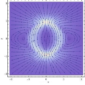
Figure 1: Density contour plot of the magnetic vector field in the plane $y=0$.

In Fig. 2.a-d the one can retrieve a non-trivial helical structure of the magnetic field. The magnetic vector field lines starting at far distance $z>>0$ approach the central area and wind around the $Z$-axis, Fig. 2a. Passing the plane $z=0.93$ the magnetic field lines are coming untwisted and moving away from the $Z$-axis, Fig. 2b,c. In the interior area $0\leq z\leq 0.93$ the magnetic fields approach the plane $z=0$ with a quite complicate helical structure which shows opposite winding directions above and below the plane $z=0$, Fig. 2d. In lower half-space the magnetic field has a similar behavior due to the reflection symmetry $z\rightarrow-z$.

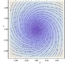
(a)  $z=1.0$

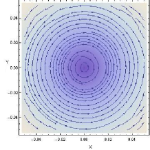
(b)  $z=0.93$

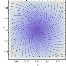
(c)  $z=0.7$

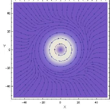
(d)  $z=+0.01$

Figure 2: Density contour plots of the magnetic field in the planes: (a) $z=1.0$; (b) $z=0.93$; (c) $z=0.7$; (d) $z=+0.01$.

The vector stream plot for the magnetic field, Fig. 3, shows the general regular structure and the presence of two local maximums of density of the magnetic field located near the $Z$-axis in the planes $z=\pm 0.93$.

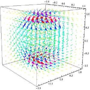
Figure 3: Three-dimensional vector stream plot for the magnetic field in Cartesian coordinates.

To make sure that magnetic field has a regular structure everywhere we make plots for the vector lines which start from four symmetric points in the upper half-space, Fig. 4. Conditionally one can select two types of magnetic vector field lines. The magnetic field lines of the first type are localized along the $Z$-axis, Fig. 4a,b, and the magnetic field lines of the second type spread to infinity along $x$ and $y$ directions.

(a)  

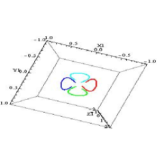
(b)  

(c)  

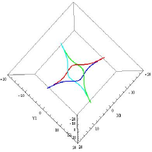
(d)  

Figure 4: (a) Vector lines for the magnetic field $H_{mn}$ starting from four symmetric points near $Z$-axis; the same lines with the point of view from above; (c) magnetic field vector lines starting from four symmetric points at large distance from $Z$-axis; (d) the same lines with the point of view from above.

One can see from Fig. 5 that field configuration has two local energy density maximums located in the planes $z=\pm 0.93$ along the circles $\theta\simeq 0.5,~{}\theta\simeq\pi-0.5$. Maximal energy density forms two tori, so the configuration can be viewed as a pair of monopole and antimonopole knots. Notice, the given monopole-antimonopole configuration has no localized magnetic charges anywhere contrary to the case of known monopole-antimonopole solutions in Yang-Mills-Higgs theory KKprd , i.e., the magnetic flux through any closed two-dimensional surface vanishes identically.

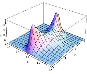
Figure 5: Energy density plot for the magnetic field in spherical coordinates $(r,\theta)$ (axially symmetric case).

In general, a detailed structure of the monopole-antimonopole configuration can vary depending on dynamics determined by the equations of motion. In the next section we will consider a more simple monopole-antimonopole solution in $CP^{1}$ model without helical structure.

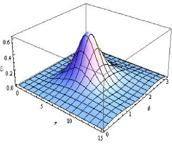
Figure 6: Energy density plot for the magnetic field configuration which minimizes the energy functional of restricted QCD.

Due to Derrick theorem derrick the simple $CP^{1}$ model with the Lagrangian (1) and the pure QCD do not admit a stable static solution. So it is unlikely that monopole can be realized as a classical solution in standard QCD. However, it is surprising that monopole-antimonopole configuration considered above provide a minimum of the energy functional for any given total energy value. So that, one can not exclude completely the possibility of existence of monopole-antimonopole solution in pure QCD. To apply minimization procedure to the energy functional it is convenient to pass to dimensionless variables $\tilde{x}^{i}$ by rescaling $x^{i}\rightarrow d\tilde{x}^{i}$ with the length parameter $d$. The trial variational functions $(F(r,\theta),~{}G(r,\theta))$ are chosen as Fourier series in $\sin k\theta,\cos l\theta$, ($k=1,3;l=2;4$), with Laguerre polynomial radial coefficient functions $L_{n}(r)$, ($n=1,...5$). In dimensionless variables the energy functional reads $(i,j=1,2,3)$

$$E = \dfrac{1}{4d}\int d^{3}\tilde{x}\tilde{H}_{ij}^{2}.$$ (26)

We impose the following boundary conditions

$$F(0,\theta) = 0,~{}~{}~{}~{}~{}G(0,\theta)=0,$$

$$F(\infty,\theta) = 1,~{}~{}~{}~{}~{}G(\infty,\theta)=1.$$ (27)

Minimizing procedure of the energy functional gives the total energy value

$$E\simeq\dfrac{4.06}{d}.$$ (28)

The energy density plot, Fig. 6, shows that the monopole and antimonopole merge together forming a toroidal structure. Since the Hopf charge is half-integer, $Q_{H}=\frac{1}{2}$, the monopole-antimonopole configuration differs from the topological knot and has non-vanishing magnetic fluxes through the upper and lower semi-spheres $H_{\pm}^{2}$ of infinite radius, (23). It is obvious that the configuration can not represent a stable solution due to presence of the scale parameter $d$ which characterizes the effective size of the monopole configuration. This is in close analogy with ’t Hooft-Polyakov monopole case where the energy of ’t Hooft-Polyakov monopole in BPS limit includes a scale parameter (averaged value of the Higgs field) and its presence destabilizes the solution.

At far distance the given magnetic field configuration is similar to a monopole-antimonopole bound state, and it does not possess a localized magnetic charge inside any closed surface. This type of solution can resolve a puzzle of existence of monopole in QCD and in electro-weak standard theory, where, as it is well known, finite energy non-composite monopole solution has not been found so far. Due to possible importance of this monopole configuration we will demonstrate the existence of such a solution in a simple $CP^{1}$ model with a potential term which determines an appropriate boundary condition at infinity.

IV Monopole-antimonopole solution in $CP^{1}$ model with a potential term

We consider monopole-antimonopole field configuration determined by winding numbers $m=1,n=2$ in a simple case when the function $f(r,\theta)$ entering the ansatz (LABEL:ansmm) vanishes identically. Let us consider the following Lagrangian for the $CP^{1}$ model with a potential term

$${\cal L} = -\dfrac{1}{4}H_{\mu\nu}^{2}-V(u),$$

$$V(u) = \dfrac{k^{2}}{4}\sin^{2}\theta\cdot$$ (29)

$$\Big{(}\dfrac{2}{2-i\sin\theta(e^{-i\phi}u-e^{i\phi}\stackrel{{\scriptstyle\ast}}{{u}})}-\dfrac{1}{2}\Big{)}^{2}.$$

Due to a special form of the chosen ansatz the potential term can be re-written in a simple form in terms of the function $G(r,\theta)$

$$V(G) = \dfrac{k^{2}}{4}\sin^{2}\theta(G-\dfrac{1}{2})^{2}.$$ (30)

The potential term provides an appropriate boundary condition for the field $G(r,\theta)$ at space infinity. A corresponding equation of motion represents a non-linear partial differential equation (pde)

$$\dfrac{1}{(1+\stackrel{{\scriptstyle\ast}}{{u}}u)^{2}}\partial_{\nu}(\sqrt{g}\partial_{\mu}uH^{\mu\nu})-\dfrac{k^{2}}{2}r^{2}\sin^{3}\theta(G-\dfrac{1}{2})$$

$$=0.$$ (31)

The reduced form of the ansatz (LABEL:ansmm) with one non-vanishing function $G$ implies the following expressions for the vector magnetic field $\vec{H}_{i}=\frac{1}{2}\epsilon_{ijk}H_{jk}$ at space infinity

$$\vec{H}_{r} = -\dfrac{2\sin(2\theta)}{(1+\sin^{2}\theta)^{2}},$$

$$\vec{H}_{\theta} = 0,~{}~{}~{}~{}~{}\vec{H}_{\varphi}=0.$$ (32)

The magnetic flux through the sphere $S^{2}$ of infinite radius gives vanishing total magnetic charge

$$\int_{S^{2}}drd\theta H_{r}=0.$$ (33)

The magnetic fluxes through the upper and lower half-spheres of $S^{2}$ are twice less compare to the monopole-antimonopole configuration considered in the previous section

$$\Phi_{+} = \int dr\int_{0}^{\frac{\pi}{2}}d\theta H_{r\theta}(\infty,\theta)=-2\pi,$$

$$\Phi_{-} = \int dr\int_{\frac{\pi}{2}}^{\pi}d\theta H_{r\theta}(\infty,\theta)=+2\pi.$$ (34)

There is no magnetic flux around the $Z$-axis, consequently, the Hopf charge density vanishes identically.

One can find solution near the origin $r\simeq 0$ and near space infinity $r\simeq\infty$ using perturbation theory. Expanding the function $G(r,\theta)$ in Taylor series

$$G(r,\theta) = g_{1}(\theta)r+g_{2}(\theta)r^{2}+g_{3}(\theta)r^{3}+...,$$ (35)

one obtains a solution near $r=0$ with the following coefficient functions up to third order of perturbation theory:

$$g_{1}(\theta) = c_{1},$$

$$g_{2}(\theta) = -(c_{1}^{2}+\dfrac{k^{2}}{256c_{1}^{2}}),$$

$$g_{3}(\theta) = \dfrac{7c_{1}^{3}+3c_{2}}{5}+\dfrac{9k^{2}}{640c_{1}}(1-\dfrac{1}{2^{10}c_{1}^{4}})$$ (36)

$$+ c_{2}\cos(2\theta),$$

where $c_{1},c_{2}$ are arbitrary integration constants. Notice the appearance of the angle dependent term in the last equation which implies that solution is axially symmetric and depends on two variables, $(r,\theta)$. In asymptotic region near space infinity, $r\simeq\infty$, one has a solution which is expressed by the series expansion (up to second order of perturbation theory)

$$G(r,\theta))=\dfrac{1}{2}+\sum_{n=1}^{\infty}b_{n}(\theta)\dfrac{1}{r^{4n}},$$

$$b_{1}(\theta)=\dfrac{2048(7+3\cos(2\theta))}{k^{2}(\cos(2\theta)-3)^{5}},$$

$$b_{2}(\theta)=\dfrac{134217728}{k^{4}(\cos(2\theta)-3)^{11}}$$

$$\cdot(119-235\cos(2\theta)-139\cos(4\theta)-9\cos(6\theta)).$$ (37)

The solution is given by asymptotic series and represents a non-perturbative solution which exists only for non-zero values of the parameter $k$. With this one can solve numerically the partial differential equation (31) imposing Neumann boundary conditions $\partial_{\theta}G(r,\theta)|_{\theta=0,\pi}=0$. The solution has been obtained by using the package COMSOL 3.5, the plot for the function $G(r,\theta)$ is depicted in Fig. 7 with the model parameter $k=2$.

Figure 7: Solution for the function $G(r,\theta)$ with the model parameter $k=2$.

Figure 8: Total energy density plot, $k=2$.

The energy density profile, Fig. 8, has one local maximum with two tails falling down at far distance. The solution represents non-helical magnetic field configuration, $\vec{H}_{\varphi}=0$.

One can solve PDE for various values of the model parameter $k$. For $k\geq 0.5$ one has good convergency properties for all solutions. The ratio of the potential energy $E_{pot}^{pde}$ to the total energy $E_{tot}^{pde}$ for various values of the parameter $k$ is near $0.44$. The obtained total energy values are in good agreement with estimates obtained by using variational method of minimizing the energy functional, see Table 1.

k	$E^{pde}_{total}$	$E_{pot}^{pde}/E_{total}^{pde}$	$E_{total}^{var}$
0.5	3.68	0.45	3.42
1	5.31	0.44	5.14
2	7.61	0.44	7.92
5	12.22	0.44	15.58

Table 1: Energy values for different values of the parameter $k$: $E_{total}^{pde},~{}E_{pot}^{pde}$ are the total and potential energies retrieved from solving pde, $E_{total}^{var}$ is the total energy obtained by using variational method

In conclusion, we have proposed a new type of finite energy monopole configuration which can be treated as a monopole-antimonopole pair. An essential feature of the configuration is that it does not possess localized magnetic charges whereas the magnetic fluxes through the upper (lower) half-spheres of infinite radius correspond to monopole (antimonopole) charge. The discrete values of the magnetic charges are conditioned by integer winding numbers $(m,n)$, whereas a helical structure of the magnetic field is provided by non-zero value of the Hopf charge. Such finite energy monopole-antimonopole configurations minimize the energy functional in restricted QCD, and they can play an important role in QCD.

The existence of monopole-antimonopole solution in a simple $CP^{1}$ model shows that the field $\hat{n}$ can regularize the singularity inherent to point like monopoles. In standard QCD the field $\hat{n}$ represents pure topological degrees of freedom, i.e., it does not have dynamic content. Due to this, rather there is no monopole solution with non-zero magnetic charge in pure QCD. However, in effective theories of QCD describing infrared limit in Faddeev-Niemi formalism FNprl99 ; shabanov the field $\hat{n}$ manifests dynamical properties. It would be interesting to study extended Skyrme-Faddeev-Niemi models with potential terms adam ; foster ; ferreira in search of possible monopole-antimonopole solutions. Another important implication of our results is related to the problem of existence monopoles in the theory of electro-weak interactions. We expect that finite energy monopole-antimonopole solution can exist within the formalism of the standard model. These issues will be considered in a subsequent paper pzzRC4 .

- (1) Y. Nambu, Phys. Rev. D10, 4262 (1974).
- (2) S. Mandelstam, Phys. Rep. 23C, 245 (1976).
- (3) A. Polyakov, Nucl. Phys. B120, 429 (1977).
- (4) P.A.M. Dirac, Phys. Rev. 74, 817 (1948).
- (5) T.T. Wu and C.N. Yang, Phys. Rev. D12, 3845 (1975).
- (6) G. t Hooft, Nucl. Phys. B79, 276 (1974).
- (7) A. M. Polyakov, JETP Lett. 20, 194 (1974).
- (8) Y. M. Cho, Phys. Rev. D21, 1080 (1980).
- (9) Y. S. Duan and Mo-Lin Ge, Sci. Sinica 11, 1072 (1979).
- (10) Y. M. Cho and D. G. Pak, Phys.Lett. B632, 745 (2006).
- (11) L. D. Faddeev, Antti J. Niemi, Phys.Rev.Lett. 82, 1624 (1999).
- (12) S. V. Shabanov, Phys. Lett. B458, 322 (1999).
- (13) Y. Nambu, Nucl. Phys. B130, 505 (1977).
- (14) D. A. Nicole, J. Phys. G4, 1363 (1978).
- (15) H. Aratyn, L. A. Ferreira and A. H. Zimerman, Phys. Rev. Lett. 83, 1723 (1999).
- (16) L. P. Zou, P. M. Zhang and D. G. Pak, Phys. Rev. D87,107701 (2013).
- (17) B. Kleihaus and J. Kunz, Phys. Rev. D61, 025003 (1999).
- (18) G. H. Derrick, J. Math. Phys. 5, 1252 (1964).
- (19) C. Adam, J. Sanchez-Guillen, T. Romanczukiewicz, A. Wereszczynski, arXiv: 0911.3673 [hep-th] (2009).
- (20) D. Foster, Phys.Rev. D83 085026 (2011).
- (21) L. A. Ferreira, J. Jaykka, N. Sawado, K. Toda, Phys. Rev. D85, 105006 (2012).
- (22) D. G. Pak, P. M. Zhang and L. P. Zou, Monopoles in Weinberg-Salam model, arXiv: 1311.7567.