Direct method for measuring purity, superfidelity, and subfidelity
of photonic two-qubit mixed states

Abstract

The Uhlmann-Jozsa fidelity (or, equivalently, the Bures distance) is a basic concept of quantum communication and quantum information, which however is very difficult to measure efficiently without recourse to quantum tomography. Here we propose a direct experimental method to estimate the fidelity between two unknown two-qubit mixed states via the measurement of the upper and lower bounds of the fidelity, which are referred to as the superfidelity and subfidelity, respectively. Our method enables a direct measurement of the first- and second-order overlaps between two arbitrary two-qubit states. In particular, the method can be applied to measure the purity (or linear entropy) of a single two-qubit mixed state in a direct experiment. We also propose and critically compare several experimental strategies for measuring the sub- and superfidelities of polarization states of photons in various linear-optical setups.

1 Introduction

Fidelity plays a fundamental role in classical CoverBook and quantum NielsenBook ; BengtssonBook communication theories as a quantitative measure of the accuracy of imperfect transmission of signals through a communication channel. Fidelity has also other basic applications in quantum information, quantum optics, and even condensed-matter physics.

The most popular definition of fidelity between two mixed quantum states $\rho_{1}$ and $\rho_{2}$ (corresponding to, e.g., the input and output states of a communication channel) was given by Uhlmann Uhlmann76 and Jozsa Jozsa94 as

$$F(\rho_{1},\rho_{2})\equiv\Big{[}{\rm Tr}\Big{(}\sqrt{\sqrt{\rho_{1}}\rho_{2}\sqrt{\rho_{1}}}\Big{)}\Big{]}^{2},$$ (1)

which is also referred to as the Uhlmann transition probability Uhlmann76 . To avoid confusion, we note that the root fidelity $\sqrt{F}$ is sometimes referred to as the fidelity (see, e.g., Ref. NielsenBook ). The fidelity vanishes for orthogonal states and is equal to 1 for identical states. If one of the states is pure, say $\rho_{1}=|\psi_{1}\rangle\langle\psi_{1}|$, then the fidelity simplifies to $F=\langle\psi_{1}|\rho_{2}|\psi_{1}\rangle$. The fidelity has a few important and useful properties including Uhlmann76 ; Jozsa94 ; Mendonca08 ; Miszczak09 (a) bounds $0\leq F(\rho_{1},\rho_{2})\leq 1$, (b) symmetry $F(\rho_{1},\rho_{2})=F(\rho_{2},\rho_{1})$, (c) unitary invariance [i.e., $F(\rho_{1},\rho_{2})=F(U\rho_{1}U^{\dagger},U\rho_{2}U^{\dagger})$ for an arbitrary unitary operator $U$], (d) multiplicativity [e.g., $F(\rho_{1}\otimes\rho_{2},\rho_{3}\otimes\rho_{4})=F(\rho_{1},\rho_{3})F(\rho_{2},\rho_{4})$], (e) concavity, and (f) joint concavity.

A physical interpretation of the fidelity as a measure of distinguishability can be given as follows Uhlmann76 ; Jozsa94 : In a decoherence scenario, based on purifications instead of collapses of states, an arbitrary mixed state $\rho_{S}$ can be given by a pure state $|\psi_{SE}\rangle$ of a subsystem $S$ entangled with some larger system (environment) $E$, which is reduced to $S$, i.e., $\rho_{S}=\mathrm{Tr}_{E}(|\psi_{SE}\rangle\langle\psi_{SE}|)$. Then the fidelity corresponds to the maximum taken over all such purifications $|\psi_{n}\rangle\equiv|\psi_{SE}^{(n)}\rangle$ of states $\rho_{n}\equiv\rho^{(n)}_{S}$ for $n=1,2$, i.e., $F(\rho_{1},\rho_{2})=\max|\langle\psi_{1}|\psi_{2}\rangle|^{2}$.

The fidelity is simply related to the Bures metric Bures69 (the Helstrom metric Helstrom67 ) as $D_{B}(\rho_{1},\rho_{2})^{2}=2[1-\sqrt{F(\rho_{1},\rho_{2})}]$, which can be considered a quantum generalization of the Fisher information metric. The Bures metric can be used to quantify quantum entanglement Vedral97 ; Marian08 , nonclassicality Marian02 , and polarization polarization . The Braunstein-Caves distinguishability metric Braunstein94 , defined via the Bures metric, is a useful tool of quantum estimation theory. Entanglement measures based on the Bures metric are also useful for identifying and characterizing quantum phase transitions, e.g., as indicators of their criticality phase_transitions .

An important question arises as to how to measure the fidelity $F(\rho_{1},\rho_{2})$ (or its bounds) between two mixed states. Obviously, one can apply a method for quantum state tomography for the complete reconstruction of the states $\rho_{1}$ and $\rho_{2}$. Then, with this knowledge, the fidelity can be calculated explicitly. However, this approach is extremely inefficient as it requires measuring redundant information to finally determine just a single value of the fidelity. Note that the fidelity, given by Eq. (1), between two mixed states is difficult not only to measure directly but even to calculate analytically. We note that analytical formulas for the fidelity are known only for a few types of states including single-qubit states BengtssonBook and multimode Gaussian states Marian12 .

In this article we show how to directly measure the super- and subfidelities which are, respectively, the upper and lower bounds on the fidelity $F(\rho_{1},\rho_{2})$ between two arbitrary two-qubit mixed states $\rho_{1}$ and $\rho_{2}$ Miszczak09 ; Zhou12 . Moreover, we describe here an experimental method for measuring the purity $\chi(\rho)$, which is a degree of information about the preparation of a quantum state $\rho$ as defined by the trace norm of $\rho$:

$$\chi(\rho)=||\rho\rho^{\dagger}||=||\rho^{2}||=\mathrm{Tr}(\rho^{2}).$$ (2)

The purity ranges from $\chi=1/d$ for completely mixed states $\rho=I/d$ of dimension $d$ to $\chi=1$ for pure states. By recalling deep mathematical and physical similarities between the classical optical polarizations and qubits, one can conclude that the classical degree of polarization and the quantum purity of a qubit are close analogs Gamel12 ; Bartkiewicz10 .

On the other hand, the lack of information about the preparation of a given state, which is referred to as the mixedness, can be quantified by entropic measures, such as the von Neumann and Bastiaans-Tsallis entropies, including the linear entropy $S_{L}=1-\chi$, which is a linear approximation to the von Neumann entropy. The linear entropy can be considered a measure of quantum entanglement of a bipartite pure state if one of the subsystems is traced out. For two-qubit mixed states, the relation between the linear entropy and (i) the von Neumann entropy, (ii) the entanglement of formation (which is a canonical measure of entanglement), and (iii) the violations of the Clauser-Horne-Shimony-Holt (CHSH) inequality were studied in, e.g., Refs. Munro01 ; Wei03 ; Peters04 . A comparative analysis of the mixedness (as measured by the linear and von Neumann entropies) and quantum noise (as described by the squeezing and Fano factors) was given in a dynamical scenario in, e.g., Ref. Bajer04 .

It is also important to note that the purity $\chi$ is a special case of the first-order overlap function

$$O(\rho_{1},\rho_{2})=\mathrm{Tr}(\rho_{1}\rho_{2}),$$ (3)

which is equivalent to the purity if $\rho_{1}=\rho_{2}$.

General methods to measure any polynomial function of a density matrix were described by Ekert et al.  Ekert02 and Brun Brun04 . While these approaches would also enable a direct measurement of the purity in a special case, it is not clear whether they enable efficient experimental implementations (except, e.g., the single-qubit purity measurements Adamson08 ). Indeed, as mentioned in Ref. Brun04 : “This proof of principle is very far from being a proof that such a measurement is practical.” These general approaches consist of using various two-qubit and single-qubit gates such as the controlled-SWAP or controlled-NOT and Hadamard gates. Note that the success probability of the discrete-variable controlled-NOT and controlled-SWAP gates with linear optics is limited, e.g., it is usually equal to 1/9 assuming no additional ancillae and feedforward (see Ref. Bartkowiak10 and references therein). Thus, a setup based on these approaches would be less efficient than specifically dedicated setups, such as the one proposed in this paper.

In this article we show how the first-order overlap $O(\rho_{1},\rho_{2})$ [and, thus, the purity $\chi(\rho)$] can be directly measured for arbitrary single- and two-qubit mixed states in a linear-optical experiment. We note that some experimental works on directly measuring the purity have already been reported by Du et al.  Du04 in liquid-state NMR systems of three spins-1/2 and, by using quantum polarization states as qubits, by Bovino et al. Bovino05 in a four-photon system, and by Adamson et al.  Adamson08 (based on the method proposed by Brun Brun04 ) in two- and three-photon systems. We note that our method requires a smaller number of detectors in comparison to, e.g., the method of Bovino et al.  Bovino05 . The problem of measuring the purity of a quantum state (and the overlap between two quantum states) within a ‘minimal’ model was theoretically studied in Ref. Tanaka13 . The first theoretical proposals for measuring the sub- and superfidelities were described in detail by Miszczak et al. Miszczak09 by applying the methods of Ekert et al. Ekert02 and Bovino et al. Bovino05 , respectively.

Our proposals for experiments on the first- and second-order overlaps are inspired by the method for the measurement of nonclassical correlations described in detail in Ref. Bartkiewicz13 , which can also be used for measuring, e.g., the degree of the CHSH inequality violation Bartkiewicz13b .

This article is organized as follows: In Sec. 2, we recall some basic definitions of the sub- and superfidelities. Moreover, we perform a Monte Carlo simulation of the fidelity as a weighted mean of these fidelity bounds. In Sec. 3, we describe direct methods for measuring the first-order overlap, purity, and superfidelity. Experimental considerations are presented in Sec. 4. In Sec. 5, we propose direct and experimentally-friendly methods for measuring the second-order overlap and the subfidelity. We conclude in Sec. 6.

2 Subfidelity, superfidelity and the estimation of fidelity

The density matrix of a single qubit in the Bloch representation can be written compactly as

$$\rho=\frac{1}{2}R_{m0}\,\sigma_{m},$$ (4)

by using the Einstein summation convention. The elements $R_{m0}=\mathrm{Tr}(\rho\sigma_{m})$ of the Bloch vector are defined by the Pauli matrices $\sigma_{m}$ for $m=0,1,2,3,$ where $\sigma_{0}=I$ is the identity operator. Furthermore, we study two-qubit (quartit) systems described by density matrices $\rho$, which are expressed in the standard Bloch representation as

$$\rho=\frac{1}{4}R_{mn}\,\sigma_{m}\otimes\sigma_{n}$$ (5)

in terms of the correlation-matrix elements $R_{mn}=\mathrm{Tr}(\rho\sigma_{m}\otimes\sigma_{n})$, with $m,n=0,...,3$. We can see that a single-qubit density matrix can be obtained after tracing out the second qubit from the two-qubit density matrix. Thus, in this article we focus on quartits, bearing in mind that the qubit case can be obtained simply after taking one of the qubits out of the picture.

Let us denote compactly $F(\rho_{1},\rho_{2})=[\mathrm{Tr}(A)]^{2},$ where $A=\sqrt{\sqrt{\rho_{1}}\rho_{2}\sqrt{\rho_{1}}}$. For single-qubit states, $A$ is a $2\times 2$ matrix, which satisfies the characteristic equation

$$A^{2}-A\mathrm{Tr}(A)+I\mathrm{det}(A)=0;$$ (6)

thus

$$F(\rho_{1},\rho_{2})=O(\rho_{1},\rho_{2})+\sqrt{[1-O(\rho_{1},\rho_{1})][1-O(\rho_{2},\rho_{2})]},$$ (7)

which can be directly measured by our proposed method.

For two-qubit (and higher-dimensional) density matrices the situation is quite different. Nevertheless, we can use the upper and lower bounds on the fidelity, given by Miszczak09 :

$$E(\rho_{1},\rho_{2})\leq F(\rho_{1},\rho_{2})\leq G(\rho_{1},\rho_{2}),$$ (8)

where

$$E(\rho_{1},\rho_{2})=\mathrm{Tr}(\rho_{1}\rho_{2})+\sqrt{2[\mathrm{Tr}(\rho_{1}\rho_{2})]^{2}-2\mathrm{Tr}[(\rho_{1}\rho_{2})^{2}]},\hskip 11.38109pt$$ (9)

$$G(\rho_{1},\rho_{2})=\mathrm{Tr}(\rho_{1}\rho_{2})+\sqrt{[1-\mathrm{Tr}(\rho_{1}^{2})][1-\mathrm{Tr(}\rho_{2}^{2})]},\hskip 28.45274pt$$ (10)

which are referred to as the subfidelity and superfidelity, respectively. These formulas can be rewritten as

$$G(\rho_{1},\rho_{2}) = O(\rho_{1},\rho_{2})+\sqrt{S_{L}(\rho_{1})S_{L}(\rho_{2})},$$ (11)

$$E(\rho_{1},\rho_{2}) = O(\rho_{1},\rho_{2})+\sqrt{2[O^{2}(\rho_{1},\rho_{2})-O^{\prime}(\rho_{1},\rho_{2})]}.\quad$$ (12)

Thus, to measure these bounds directly, we need to measure the first-order overlap $O(\rho_{1},\rho_{2})$, given by Eq. (3), and the second-order overlap

$$O^{\prime}(\rho_{1},\rho_{2}) = \mathrm{Tr}(\rho_{1}\rho_{2}\rho_{1}\rho_{2}),$$ (13)

together with the linear entropies (purities), $S_{L}(\rho_{n})=1-O(\rho_{n},\rho_{n})$ (for $n=1,2$), which are the special cases of $O(\rho_{1},\rho_{2})$. Let us note that if (at least) one of the states $\rho_{1},\rho_{2}$ is pure, then the superfidelity is equal to the fidelity and is given only by the first term, i.e., the overlap $O(\rho_{1},\rho_{2})$. Thus, after finding that either $\rho_{1}$ or $\rho_{2}$ is pure, the fidelity can be found by measuring the overlap $O(\rho_{1},\rho_{2})$ only.

In any other case the fidelity $F$ can be estimated as an average of the subfidelity $E$ and superfidelity $G$ with some certain error. The error can be minimized in two ways: (i) by finding tighter measurable bounds on the fidelity or (ii) by using the best expression for the mean value (arithmetic, harmonic, geometric, etc.). In our article we focus only on this second aspect and numerically optimize the generalized mean (power mean) defined as

$$\bar{F}(\rho_{1},\rho_{2})=\big{[}wE^{m}(\rho_{1},\rho_{2})+(1-w)G^{m}(\rho_{1},\rho_{2})\big{]}^{\frac{1}{m}},$$ (14)

which for balanced weights $w=1-w=1/2$, and in special cases for $m=-1,0,1$, becomes the harmonic, geometric, and arithmetic mean, while for $m=-\infty,\infty$ it reduces to $\bar{F}=E,G$, respectively. Thus, the generalized mean is bounded from below by $E$ and from above by $G$, i.e., for $m\in(-\infty,\infty)$

$$E(\rho_{1},\rho_{2})\leq\bar{F}(\rho_{1},\rho_{2})\leq G(\rho_{1},\rho_{2}).$$ (15)

From our Monte Carlo simulation for $10^{7}$ pairs of random two-qubit states (as shown in Fig. 1) we found with the method of least squares that the optimal $m=-2.13$ and $w=0.568$ providing the smallest estimation error $\Delta=\sqrt{\langle(\bar{F}-F)^{2}\rangle}=0.0278$, which is an improvement in comparison to the arithmetic mean providing $\Delta=0.0652$. Our method of calculating means is not the most general one (e.g., one can use a generalized $f$ mean). However, one must remember that true fidelity values are to be found between $E$ and $G$, so the maximal estimation error is greater than the error average.

We focus on the analysis of nonlinear properties of two-qubit states because they play an important role in quantum protocols exploiting quantum correlations. Thus, establishing methods of testing various properties of these states is well motivated. This is especially important for photonic qubits since photons are typical carriers of quantum information used in quantum communication protocols.

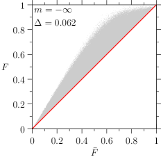
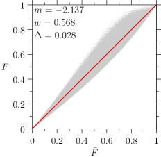
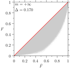
Figure 1: (Color online) Fidelity $F(\rho_{1},\rho_{2})$ versus generalized mean $\bar{F}(\rho_{1},\rho_{2})$, corresponding to (a) subfidelity $E(\rho_{1},\rho_{2})$ for $m=-\infty$, (b) optimized mean for $m=-2.137$, (c) arithmetic mean for $m=1$, and (d) superfidelity $G(\rho_{1},\rho_{2})$ for $m=+\infty$, as calculated in our Monte-Carlo simulation for $10^{7}$ pairs of two-qubit states. The estimation error is given by $\Delta=\sqrt{\langle(\bar{F}-F)^{2}\rangle}$. Note that if the fidelity bounds $E$ and $G$ were tighter, then the area covered by the simulation outcomes would be smaller converging to the $G=E$ line.

3 Efficient measurements of first-order overlap, purity, and superfidelity

The purity $\chi$ can be observed directly if we assume that we have access to two copies of the two-qubit system. The first-order overlap (or the purity in the special case for $\rho_{1}=\rho_{2}$) can be calculated directly as

$$O(\rho_{1},\rho_{2})=\frac{1}{16}R^{(1)}_{mn}R^{(2)}_{kl}\mathrm{Tr}[(\sigma_{m}\sigma_{k})\otimes(\sigma_{k}\sigma_{l})],$$ (16)

where $R^{(k)}$ are the correlation matrices of $\rho_{k}$ for $k=1,2$, as defined below Eq. (5). The multiplication of the Pauli matrices is given as

$$\sigma_{a}\sigma_{b}=i\varepsilon_{abc}\sigma_{c}+\delta_{ab}\sigma_{0},$$ (17)

where $i$ is the imaginary unit, $\delta_{ab}$ is the Kronecker $\delta$, and $\varepsilon_{abc}$ is the Levi-Civita symbol, which is $\varepsilon_{abc}=0$ if $a\times b\times c=0$ or at least two indices are equal. Note that $\sigma_{n}$ matrices are traceless except for $n=0$; thus

$$\mathrm{Tr}(\sigma_{a}\sigma_{b})=2\delta_{ab}.$$ (18)

Hence, we can rewrite Eq. (16) as

$$O(\rho_{1},\rho_{2})=\frac{1}{4}R^{(1)}_{mn}R^{(2)}_{mn}.$$ (19)

We can express $R^{(k)}_{mn}$ as expectation values of the Pauli matrices:

$$R^{(1)}_{mn} = \mathrm{Tr}[(\sigma_{m}\otimes\sigma_{n})\rho_{1}],$$ (20)

$$R^{(2)}_{mn} = \mathrm{Tr}[(\sigma_{m}\otimes\sigma_{n})\rho_{2}],$$ (21)

hence

$$O(\rho_{1},\rho_{2}) = \frac{1}{4}\mathrm{Tr}[(\sigma_{m}\otimes\sigma_{n}\otimes\sigma_{m}\otimes\sigma_{n})(\rho_{1}\otimes\rho_{2})]$$ (22)

$$= \frac{1}{4}\mathrm{Tr}[(\sigma_{m}\otimes\sigma_{m})\otimes(\sigma_{n}\otimes\sigma_{n})(\rho_{1}\otimes\rho_{2})^{\prime}]$$

$$= \frac{1}{4}\mathrm{Tr}[(V_{A_{1}A_{2}}\otimes V_{B_{1}B_{2}})^{\prime}(\rho_{1}\otimes\rho_{2})],$$

where $V=\sigma_{m}\otimes\sigma_{m}=2I^{\otimes 2}-4|\Psi^{-}\rangle\langle\Psi^{-}|$, with $|\Psi^{-}\rangle$ denoting the singlet state, and $(\rho_{1}\otimes\rho_{2})^{\prime}=S_{A_{2}B_{1}}(\rho_{1}\otimes\rho_{2})S_{A_{2}B_{1}}$. The self-adjoint transformation $S_{A_{2}B_{1}}=I\otimes S\otimes I$ is the operation swapping modes $A_{2}$ and $B_{1}$, which is given in terms of the SWAP operator

$$S=\left(\begin{array}[]{cccc}1&0&0&0\\ 0&0&1&0\\ 0&1&0&0\\ 0&0&0&1\end{array}\right).$$ (23)

We can now introduce the Hermitian overlap operator

$$\Gamma=S_{A_{2}B_{1}}V_{A_{1}A_{2}}V_{B_{1}B_{2}}S_{A_{2}B_{1}},$$ (24)

which, if measured on $\rho_{1}\otimes\rho_{2}$, provides the value of the overlap $O(\rho_{1},\rho_{2})$ and, in the special case, the purity if $\rho_{1}=\rho_{2}$. Hence, the overlap is a real observable measured on a system consisting of two copies of the investigated state $\rho$. Let us note that measuring the purity is, thus, equivalent to measuring a product of $V$ operators, which was shown in Ref. Bartkiewicz13 to be experimentally accessible using linear optics. If the two-qubit state is produced at frequency $1/\tau$, we delay every second state $\rho$ and we can measure the product of $V$ operators directly as shown in Fig. 2.

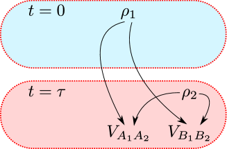
Figure 2: (Color online) Method for a single iteration of the measurement of the overlap $\mathrm{Tr}(\rho_{1}\rho_{2})$ (and, in a special case, the purity $\chi$ and linear entropy $S_{L}=1-\chi$) between any two-qubit states $\rho_{1}$ and $\rho_{2}$ produced at constant time intervals $\tau$. The subsystem of the first (second) qubit is called $A$ ($B$). The measurement should be repeated until some large enough number $K$ of values is accumulated. The delay is implemented at times $t=2k\tau$, where $k=0,1,2,...,K-1$ and $2K\tau$ is the duration of the measurement. The delay can be implemented using fast switching between, e.g., two paths of the optical-length difference corresponding to delay $\tau$. This method works also if the states $\rho_{1}$ and $\rho_{2}$ are qubits given that we removed the measurement $V_{B_{1}B_{2}}$ or $V_{A_{1},A_{2}}$.

The setup shown in Fig. 3 can be used in a direct measurement of the overlap (thus, also of the linear entropy) of a two-qubit state, since $O(\rho_{1},\rho_{2})=\langle\Gamma\rangle=\mathrm{Tr}[(V_{A_{1}A_{2}}\otimes V_{B_{1}B_{2}})(\rho_{1}\otimes\rho_{2})^{\prime}]/4$. The possible outcomes for a single measurement instance are $a_{k}=-8,0,4,16$, which are the products of two outcomes of the coincidence detections in the left and right arms of the setup in Fig. 3 marked as $-4,0,2$. The outcome $2$ is assigned to the coincidence detection in the outermost detectors of the $V$ blocks, $-4$ for the coincidence detection in the middle detectors, and $0$ if neither of the two coincidences has been detected. Useful values of $a_{k}$ appear for $K_{0}=\eta^{4}K/4$ of the cases when the states $\rho_{1}$ and $\rho_{2}$ are delivered, assuming that $\eta$ is the quantum efficiency of the detectors. The obtained expectation value of the overlap reads

$$O(\rho_{1},\rho_{2})=\langle\Gamma\rangle\approx\frac{1}{4K_{0}}\sum_{k=1}^{K}a_{k},$$ (25)

where

$$K_{0}=\sum_{k=1}^{K}\delta_{a_{k},4}$$ (26)

and $\delta_{a_{k},4}$ is the Kronecker $\delta$. As for any measurement, equality is reached in the limit of $K_{0}\to\infty$. Thus, we have demonstrated how the first-order overlap $O(\rho_{1},\rho_{2})$ and the purity $\chi$ can be measured directly.

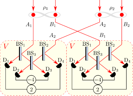
Figure 3: (Color online) Setup implementing a direct measurement of the first-order overlap $O(\rho_{1},\rho_{2})=\mathrm{Tr}(\rho_{1}\rho_{2})$ between arbitrary two-qubit mixed states $\rho_{1}$ and $\rho_{2}$. The setup consists of two $V$ blocks as in Ref. Bartkiewicz13 . Due to the probabilistic nature of the path taken by photons after the BS interaction the setup can provide conclusive results in at most $1/4$ of the cases when $\rho_{1}$ and $\rho_{2}$ are delivered (as discussed in Fig. 2). This maximum performance is achieved when the photons are deterministically antibunched (i.e., always projected onto the singlet state) if both of them impinge on BS₃. Note that the BSs are asymmetric, i.e., the photon is phase shifted by $\pi$ only when reflected from the black-shaded side of the BSs. If $\rho_{1}$ and $\rho_{2}$ are single photons then only one $V$ block is required and the measurement setup corresponds to the one used in Ref. Hendrych03 .

4 Experimental considerations

The setup in Fig. 3 provides a simple way to understand how the entire purity measurement protocol works. It is, however, impractical from the experimental point of view. First of all, it requires eight detectors that have to be calibrated to give the same detection efficiency. Further, to do that, it requires also six beam splitters (BSs) that have to be well adjusted in a real experimental setup, and even if this could be done, their number diminishes the effectiveness of the protocol. The setup, as depicted in Fig. 3, gives the maximum success probability (conclusive coincidences) in 1/4 of the cases when all photons are delivered. This value can be increased together with experimental simplification of the procedure in several ways. In this section we discuss several strategies experimentally suitable for various linear-optical platforms.

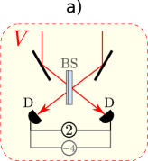
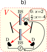
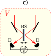
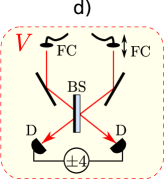
Figure 4: (Color online) Experimentally friendly methods for the measurement of the $V$ block as described in the text based on (a) a removable beam splitter, (b) a Mach-Zehnder interferometer, (c) a partially movable beam splitter, and (d) two-photon overlap alignment. BS, balanced beam splitter, PS, phase shifter, FC, fiber coupler, and D, detector. Motorized translation (double arrow) is used to tune the temporal delay between the photons in order to switch between the measurement regimes as explained in the text.

The first strategy involves just a removable beam splitter and a pair of detectors [see Fig. 4(a)]. In this case, one inserts a balanced beam splitter to the setup for a half of the measurement time (assuming that photons are distributed uniformly in time). Thus, the singlet-state projection is performed with the beam splitter inserted, while the identity projection with the beam splitter removed. As in the original method, the coincidence counts with the beam splitter are attributed to the value $(-4)$, while those without the beam splitter are multiplied by the value of 2. The effectiveness of this method, as defined in the caption of Fig. 3, reaches 1. Also the number of beam splitters is reduced to two (one for each $V$ block), while the number of detectors is reduced to four. Unfortunately, this strategy would not be very experimentally friendly in the case of bulk or integrated optics. On both these platforms, removing and reinserting the beam splitter is accompanied by a demanding adjustment especially if the beam splitter has to be as balanced as possible. In fiber-optics, this strategy can be implemented more easily with beam splitters with a tunable splitting ratio Bartuskova07 .

The second strategy is a generalization of the first strategy bringing it closer to automation. It is depicted in Fig. 4(b) and it involves using a Mach-Zehnder interferometer that effectively implements a tunable beam splitter. By changing the phase from 0 to $\pi/2$ in the interferometer, one can achieve a splitting ratio in the range from 50:50 to 0:100. This technique is particularly suitable for integrated optics Smith09 . In bulk optics and fiber-optics it is impractical because of the experimental demands on keeping the phase in the interferometer stable through the entire measurement. Note that the number of beam splitters is reduced to four and so is the number of detectors. The observed coincidences with the interferometer set to the 50:50 ratio are multiplied by $(-4)$ and those in the 0:100 regime are multiplied by 2. The maximum success probability of this strategy is 1.

The third strategy is also a modification of the first one with the exception that the beam splitter is not be removed completely, but just shifted in one direction as depicted in Fig. 4(c). In our experience, this technique is particularly useful in bulk optics. After shifting the beam splitter out of its position, the reflected light no longer couples to the detectors while the transmitted light still does. Thus, we can effectively reach the splitting ratio 0:100, even with a balanced beam splitter at the expense of some losses. The readjustment of the beam splitter back to its balanced position is easily done using a good quality translation stage. As in the first strategy, the number of detectors needed is four and the number of beam splitters is two. Since only 1/4 of the impinging photons reach the detectors if the beam splitter is shifted out (in), we just multiply the number of such coincidences by 8 (-4) assuming that the measurements with the beam splitter in and out take the same time. This technique has been used in several of our experiments to measure technological losses in bulk setups Lemr11cpg ; Lemr12clone . It is, however, not suitable for integrated optics and fiber optics. Its overall maximal success probability is 5/8.

The last strategy to be discussed in this section is depicted in Fig. 4(d). It involves a fixed balanced beam splitter and a pair of detectors in each $V$ block. In order to implement singlet-state projection, two-photon overlap, corresponding to Hong-Ou-Mandel interference Hong87 , is obtained by suitable position of the translation stage holding the output couplers. On the other hand, the intensity projection is implemented by deliberate misalignment of the output coupler position so that the photons are separated in time by a duration much longer than their coherence time Halenkova12appl . Since the two-photon overlap has to be adjusted anyway, a motorized translation stage is an experimental necessity. With respect to that, this strategy does not impose any new demands on the experimental setup. The efficiency of this technique gives a success probability of 3/4 since with the misaligned overlap, the photons mark coincidence in only one-half of the cases. Assuming the same measurement time with the output couplers aligned and misaligned, the coincidences in the aligned position are multiplied by $(-4),$ while those in the misaligned position are multiplied by 4 in order to take into account the probabilistic nature of such events.

5 Efficient measurements of second-order overlap and subfidelity

Measuring the first-order overlaps $O(\rho_{1},\rho_{2})$, $\chi(\rho_{1})=O(\rho_{1},\rho_{1})$, and $\chi(\rho_{2})=O(\rho_{2},\rho_{2})$ is enough for determination of the superfidelity $G(\rho_{1},\rho_{2})$. If it is known that one of the states is pure, then we do not need to proceed with estimating the subfidelity because in this case we already have all the data needed for calculating the fidelity $F(\rho_{1},\rho_{2})=O(\rho_{1},\rho_{2})$.

In the simplest qubit case, the superfidelity and fidelity are equivalent, i.e., $G(\rho_{1},\rho_{2})=F(\rho_{1},\rho_{2})$ and no further work is required for estimating the fidelity. However, in the case of quartits one also has to estimate the subfidelity $E(\rho_{1},\rho_{2})$ to know in what range the fidelity $F(\rho_{1},\rho_{2})$ falls. The only missing quantity needed for estimating the subfidelity $E(\rho_{1},\rho_{2})$ is the second-order overlap $O^{\prime}(\rho_{1},\rho_{2})$, which depends on the Hilbert-space dimension of a given system (i.e., qubit or quartit) and requires from four to eight photons.

So, our goal now is to describe a method for measuring the second-order overlap $O^{\prime}(\rho_{1},\rho_{2})$. We know that $(\rho_{1}\rho_{2})^{2}=\frac{1}{256}R^{(1)}_{ma}R^{(2)}_{nb}R^{(1)}_{kc}R^{(2)}_{ld}(\sigma_{m}\sigma_{n}\sigma_{k}\sigma_{l})\otimes(\sigma_{a}\sigma_{b}\sigma_{c}\sigma_{d})$ and it can be verified that

$$\mbox{Tr }(\sigma_{m}\sigma_{n}\sigma_{k}\sigma_{l})=\mathcal{K}_{mnkl}\,,$$ (27)

where

$$\tfrac{1}{2}\mathcal{K}_{mnkl} = \delta_{mn}\delta_{kl}+\delta_{nk}\delta_{ml}-\delta_{mk}\delta_{nl}+2\delta_{m0}\delta_{nl}\delta_{mk}$$ (28)

$$+2\delta_{l0}\delta_{nl}\delta_{mk}-4\delta_{m0}\delta_{n0}\delta_{k0}\delta_{l0}+i\delta_{m0}\varepsilon_{nkl}$$

$$+i\delta_{n,0}\varepsilon_{klm}+i\delta_{k0}\varepsilon_{lmn}+i\delta_{l0}\varepsilon_{mnk}\$$

is the kernel for which we describe the measurement method. So, the investigated quantity reads

$$\mbox{Tr }(\rho_{1}\rho_{2})^{2} = \frac{1}{256}\mathcal{K}_{mnkl}\mathcal{K}_{abcd}$$ (29)

$$\times\mbox{Tr }(\gamma_{mnkl}\otimes\gamma_{abcd})(\rho_{1}\otimes\rho_{2})^{\otimes 2},\quad$$

where $\gamma_{mnkl}=\sigma_{m}\otimes\sigma_{n}\otimes\sigma_{k}\otimes\sigma_{l}$. In order to design an efficient setup we have to calculate

$$H=\frac{1}{16}\mathcal{K}_{mnkl}\gamma_{mnkl},$$ (30)

and find the most convenient permutation of the qubits comprising the eight-qubit system. This is because

$$\mbox{Tr }(\rho_{1}\rho_{2})^{2}=\mbox{Tr }[(H\otimes H)_{A_{1}A_{2}A_{3}A_{4}B_{1}B_{2}B_{3}B_{4}}$$

$$\times(\rho_{1}\otimes\rho_{2}\otimes\rho_{1}\otimes\rho_{2})_{A_{1}B_{1}A_{2}B_{2}A_{3}B_{3}A_{4}B_{4}}].$$ (31)

The matrix $H$ is a permutation, so it can be decomposed into a product of inversions, i.e., the SWAP operations. Note that the $V$ matrix is equivalent to the SWAP operation (see also Ref. Ekert02 ) as $V=2S$. The result reads $(S_{34}S_{23})H(S_{23}S_{34})=\frac{1}{8}S_{23}(V_{12}\otimes V_{34})S_{23}V_{34}$. Thus, we have

$$\mbox{Tr }(\rho_{1}\rho_{2})^{2} = \tfrac{1}{64}\mbox{Tr }\{[(V^{\otimes 2})^{\prime}(I\otimes V)]^{\otimes 2}(\rho_{1}\otimes\rho_{2}\otimes\rho_{1}\otimes\rho_{2})^{\prime}\}$$

$$= \tfrac{1}{64}\mbox{Tr }\{[(I\otimes V)(V^{\otimes 2})^{\prime}]^{\otimes 2}(\rho_{1}\otimes\rho_{2}\otimes\rho_{1}\otimes\rho_{2})^{\prime}\},$$

where $I$ in this section is the two-qubit identity operator,$(\rho_{1}\otimes\rho_{2}\otimes\rho_{1}\otimes\rho_{2})^{\prime}=(\rho_{1}\otimes\rho_{1}\otimes\rho_{2}\otimes\rho_{2})_{A_{1}B_{1}A_{2}B_{2}A_{3}B_{3}A_{4}B_{4}}$ and the second-order overlap operator reads $[(V^{\otimes 2})^{\prime}(I\otimes V)]^{\otimes 2}=[(V^{\otimes 2})_{A_{1}A_{3}A_{2}A_{4}}(I\otimes V)_{A_{1}A_{2}A_{3}A_{4}}]\otimes[(V^{\otimes 2})_{B_{1}B_{3}B_{2}B_{4}}(I\otimes V)_{B_{1}B_{2}B_{3}B_{4}}]$, which is a product of two Hermitian operators that commute [see Eq. (LABEL:Eq:32)] for the input state $(\rho_{1}^{\otimes 2}\otimes\rho_{2}^{\otimes 2})_{A_{1}B_{1}A_{2}B_{2}A_{3}B_{3}A_{4}B_{4}}$, thus one can measure these two operators subsequently. In the final step we just need to express $I\otimes V$ as $I\otimes V=2I^{\otimes 2}-4I\otimes P^{-}$, where $P^{-}$ is the singlet-state projection that can be performed by a beam splitter. Thus, as shown in Fig. 5, we can perform the measurement using the approach discussed in the previous section. Here the beam splitter is placed at or removed to the mixed modes $A_{3}$ and $A_{4}$, or $B_{3}$ and $B_{4}$. For each of the four cases, the final step consists of performing the measurement on four $V$ boxes. Note that the problem of measuring the second-order overlap is equivalent to the problem of measuring a first-order overlap of four-qubit states (i.e., a 16-level qudit or quantum hex).

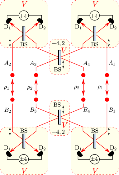
Figure 5: (Color online) Proposal of the measurement setup for the second-order overlap $O^{\prime}(\rho_{1},\rho_{2})$ for two-qubit states. The input is given as $(\rho_{1}\otimes\rho_{1}\otimes\rho_{2}\otimes\rho_{2})_{A_{1}B_{1}A_{2}B_{2}A_{3}B_{3}A_{4}B_{4}}$. If the states are single-qubit states then one of the blocks can be removed. Note that in our optimized methods (as described in Sec. 4), the number of required detectors is equal to the number of photons. Double arrows indicate the two-photon overlap alignment as in Fig. 4(d).

From the experimentalist point of view, the setup presented in this section is based on our fourth strategy as described in Sec. 4. This particular choice of implementation technique can be useful in bulk optics, where motorized translation with a range on the order of centimeters is often used to stabilize the two-photon overlap. On the other hand, for fiber and integrated optics implementations, this technique might not be practical. However, it is straightforward to swap the $V$ blocks in the proposed setup for any of the four alternative implementations of the $V$ blocks proposed in Sec. 4. The functionality of the setup remains unaffected by this replacement.

6 Conclusions

We proposed an effective and direct method for estimating the bounds of the Uhlmann-Jozsa fidelity (or, equivalently, the Bures distance) for two unknown mixed two-qubit states without recourse to quantum state tomography. Namely, we described how to measure the superfidelity and subfidelity, which are the upper and lower bounds of the fidelity, respectively Miszczak09 . We showed explicitly that the overlap of two density matrices is an observable which has its own Hermitian operator $\Gamma$, given by Eq. (24), and furthermore can be directly measured in a linear-optical experiment. Our method for the determination of the superfidelity is based on the measurement of the first-order overlap. In a special case, the method can be used for measuring the purity (or linear entropy) of a mixed two-qubit state. On the other hand, our proposal of a experimentally-friendly method for direct measuring the second-order overlap of two arbitrary two-qubit states enables the determination of their subfidelity.

Concerning the purity measurement, it is worth referring to Ref. Hendrych03 , where its authors make use of Hong-Ou-Mandel interference and a singlet-state projection performed by a balanced beam splitter to determine the two-photon overlap. In a special case this technique can be adapted for measuring the purity of a single qubit. A similar setup was used in Ref. Adamson08 , where the authors described direct and indirect purity measurements of a single qubit. They presented two separate strategies, one corresponding to a direct measurement using many consecutive pairs of the investigated state and the second corresponding to the standard quantum state tomography based on polarization projection measurements. Since the authors of Ref. Adamson08 were dealing with the measurement of single qubits, their setup requires fewer resources than the scheme presented in our paper dedicated to two-qubit purity measurements.

Our $V$ block is in fact the Hong-Ou-Mandel dip known since the famous experiment of Ref. Hong87 . Indeed, the Hong-Ou-Mandel two-photon interferometer has been used to implement a projection on a singlet state, for instance, in Ref. Hendrych03 . On the other hand, with the development of experimental techniques, the four alternative implementations of the $V$ block suitable for various platforms (including bulk, fiber, and integrated optics) have their merit.

As mentioned before, a few experiments on single-qubit purity have already been performed but, since there are additional interesting features (including entanglement) arising from the transition from one to two qubits, our proposals for direct measurement of the two-qubit purity can be an important tool for future investigations in quantum optical engineering and information processing.

Concerning the two-photon overlap measurements, we note another formal method of Ekert et al.  Ekert02 based on programmable quantum networks with controlled-SWAP gates for estimating both linear and nonlinear functionals of arbitrary states. As shown explicitly by Miszczak et al.  Miszczak09 , this network method also enables the measurement, in a special case, of the first- and second-order overlaps between a pair of two-qubit states for the estimation of their fidelity bounds. This formal method, although in principle scalable for any number of qubits, has not been applied (even theoretically) to any physical system. In contrast, we apply a purely algebraic method for estimating some specific functionals of states and describe an experimentally-friendly linear-optical implementation of our method. As in these related works Ekert02 ; Miszczak09 , we assumed that we have access to two copies of a given quantum state, which can be implemented either by producing two identical states simultaneously, or by storing the state produced earlier in order to measure it together with the second copy of the state available later. Concerning the optical measurement of the purity, our proposal requires fewer experimental resources than of Bovino et al. Bovino05 . Specifically, our setup requires only four instead of six detectors and only two beam splitters instead of four used in Ref. Bovino05 . Every additional experimental resource complicates the operation of the setup and is a possible source of imperfections.

In Sec. 4 we have presented several experimentally-friendly strategies based on our original method. All these setups represent a viable alternative to be considered in practical experimental implementations of the protocol. We cannot claim that one of them is superior to the others since each of them has its advantages and drawbacks. The choice would depend on the preferred features. For instance, if the success rate is an issue, experimentalists would probably choose the second strategy (with a success rate up to 1). On the other hand, for the highest experimental stability and precision (in bulk optics, rather than in fiber optics), the fourth strategy might be selected. Moreover, the third strategy would be a good choice for a fiber-optical implementation, while the second strategy can be suitable for integrated optics.

Moreover, we performed a Monte Carlo simulation of $10^{7}$ mixed two-qubit states and applied the method of least squares to estimate the fidelity as a generalized power mean of these fidelity bounds with the minimum average estimation error.

Experimentalists frequently use the fidelity (usually determined by applying quantum tomography) as a measure of the quality of their achievements. Remarkable progress has been observed over the past decade as the reported experimental values increased from 0.58 to 0.98.

However, it should be stressed that both the purity and fidelity are important parameters for characterizing experimental achievements with respect to quantum operations. The purity alone would not be adequate to describe how well the gate performs the requested task (for instance the controlled NOT operation). Similarly to that, the fidelity can be indeed rather high even though the purity has dropped and therefore the gate is misaligned, which typically occurs in the case of active stabilization issues. As pointed out recently in Ref. Dodonov12 to have 98% fidelity is not enough to be sure that the two states are indeed similar or close to each other. The answer depends on the specific situation and additional information about the state is needed.

We hope that this paper can stimulate further experimental interest in determining both the fidelity and purity for the purposes of quantum engineering and quantum information processing.

- (1) T. Cover and J. Thomas, Elements of Information Theory (Wiley, New York, 1991).
- (2) M. A. Nielsen and I. L. Chuang, Quantum Computation and Quantum Information (Cambridge University Press, Cambridge, 2000).
- (3) I. Bengtsson and K. Życzkowski, Geometry of Quantum States: An Introduction to Quantum Entanglement (Cambridge University Press, Cambridge, 2006).
- (4) A. Uhlmann, Rep. Math. Phys. 9, 273 (1976).
- (5) R. Jozsa, J. Mod. Opt. 41, 2315 (1994).
- (6) P. E. M. F. Mendonca, R. d. J. Napolitano, M. A. Marchiolli, C. J. Foster, and Y.-C. Liang, Phys. Rev. A78, 052330 (2008).
- (7) J. A. Miszczak, Z. Puchała, P. Horodecki, A. Uhlmann, and K. Życzkowski, Quantum Inf. Comp. 9, 0103 (2009).
- (8) D. Bures, Trans. Am. Math. Soc. 135, 199 (1969).
- (9) C. W. Helstrom, Phys. Lett. A 25, 101 (1967).
- (10) V. Vedral, M. B. Plenio, M. A. Rippin, and P. L. Knight, Phys. Rev. Lett. 78, 2275 (1997).
- (11) P. Marian and T. A. Marian, Phys. Rev. A77, 062319 (2008).
- (12) P. Marian, T. A. Marian, and H. Scutaru, Phys. Rev. Lett. 88, 153601 (2002).
- (13) A. B. Klimov, L. L. Sanchez-Soto, E. C. Yustas, J. Soderholm, and G. Bjork, Phys. Rev. A72, 033813 (2005); A. Luis, Opt. Commun. 273, 173 (2007); I. Ghiu, G. Bjork, P. Marian, and T. A. Marian, Phys. Rev. A82, 023803 (2010).
- (14) S. L. Braunstein and C. M. Caves, Phys. Rev. Lett. 72, 3439 (1994).
- (15) P. Zanardi, M. G. A. Paris, and L. C. Venuti, Phys. Rev. A78, 042105 (2008); S. J. Gu, Int. J. Mod. Phys. B 24, 4371 (2010).
- (16) P. Marian and T. A. Marian, Phys. Rev. A86, 022340 (2012).
- (17) T. Zhou and Y. Li, J. Phys. A 45, 195302 (2012).
- (18) O. Gamel and D. F. V. James, Phys. Rev. A86, 033830 (2012).
- (19) K. Bartkiewicz and A. Miranowicz, Phys. Rev. A82, 042330 (2010).
- (20) W. J. Munro, D. F. V. James, A. G. White, and P. G. Kwiat, Phys. Rev. A64, 030302 (2001).
- (21) T. C. Wei, K. Nemoto, P. M. Goldbart, P. G. Kwiat, W. J. Munro, and F. Verstraete, Phys. Rev. A67, 022110 (2003).
- (22) N. A. Peters, T. C. Wei, and P. G. Kwiat, Phys. Rev. A70, 052309 (2004).
- (23) J. Bajer, A. Miranowicz, and M. Andrzejewski, J. Opt. B 6, 387 (2004).
- (24) A. K. Ekert, C. Moura Alves, D. K. L. Oi, M. Horodecki, P. Horodecki, and L. C. Kwek, Phys. Rev. Lett. 88, 217901 (2002).
- (25) T. A. Brun, Quantum Inf. Comput. 4, 401 (2004).
- (26) R. B. A. Adamson, L. K. Shalm and A. M. Steinberg, Phys. Rev. A 75, 012104 (2007).
- (27) M. Bartkowiak and A. Miranowicz, J. Opt. Soc. Am. B 27, 2369 (2010).
- (28) J. Du, P. Zou, D. K. L. Oi, X. Peng, L. C. Kwek, C. H. Oh, and A. Ekert, arXiv:quant-ph/0411180v2
- (29) F. A. Bovino, G. Castagnoli, A. Ekert, P. Horodecki, C. M. Alves, and A. V. Sergienko, Phys. Rev. Lett. 95, 240407 (2005).
- (30) T. Tanaka, G. Kimura, and H. Nakazato, Phys. Rev. A87, 012303 (2013).
- (31) K. Bartkiewicz, K. Lemr, A. Černoch, and J. Soubusta, Phys. Rev. A87, 062102 (2013).
- (32) K. Bartkiewicz, B. Horst, K. Lemr, and A. Miranowicz, Phys. Rev. A 88, 052105 (2013)
- (33) M. Hendrych, M. Dušek, R. Filip, and J. Fiurášek, Phys. Lett. A 310, 95 (2003).
- (34) L. Bartušková, M. Dušek, A. Černoch, J. Soubusta, and J. Fiurášek, Phys. Rev. Lett. 99, 120505 (2007).
- (35) B. J. Smith, D. Kundys, N. Thomas-Peter, P. G. R. Smith, and I. A. Walmsley, Opt. Express 17, 13516 (2009).
- (36) K. Lemr, A. Černoch, J. Soubusta, K. Kieling, J. Eisert, and M. Dušek, Phys. Rev. Lett. 106, 013602 (2011).
- (37) K. Lemr, K. Bartkiewicz, A. Černoch, J. Soubusta, and A. Miranowicz, Phys. Rev. A 85, 050307(R) (2012); K. Bartkiewicz, K. Lemr, A. Černoch, J. Soubusta, and A. Miranowicz, Phys. Rev. Lett. 110, 173601 (2013).
- (38) C. K. Hong, Z. Y. Ou, and L. Mandel, Phys. Rev. Lett. 59, 2044 (1987).
- (39) E. Halenková et al., App. Opt. 51, 474 (2012).
- (40) V. V. Dodonov, J. Phys. A 45, 032002 (2012).