Abstract

We investigate the predictions for neutrinoless double beta ($(\beta\beta)_{0\nu}$-) decay effective Majorana mass $\left|\langle\!~{}m~{}\!\rangle\right|\$ in the $3+1$ and $3+2$ schemes with one and two additional sterile neutrinos with masses at the eV scale. The two schemes are suggested by the neutrino oscillation interpretation of the reactor neutrino and Gallium “anomalies” and of the data of the LSND and MiniBooNE experiments. We analyse in detail the possibility of a complete or partial cancellation between the different terms in $\left|\langle\!~{}m~{}\!\rangle\right|\$, leading to a strong suppression of $\left|\langle\!~{}m~{}\!\rangle\right|\$. We determine the regions of the relevant parameter spaces where such a suppression can occure. This allows us to derive the conditions under which the effective Majorana mass satisfies $\mbox{$\left|\langle\!~{}m~{}\!\rangle\right|\ $}>0.01$ eV, which is the range planned to be exploited by the next generation of $(\beta\beta)_{0\nu}$-experiments.

1 Introduction

All compelling neutrino oscillation data can be described within the reference 3-flavour neutrino mixing scheme with 3 light neutrinos $\nu_{j}$ having masses $m_{j}$ not exceeding approximately 1 eV, $m_{j}\ \raisebox{-1.72218pt}{\hbox to0.0pt{$\sim$\hss}}\raisebox{1.72218pt}{$<$}\ 1$ eV, $j=1,2,3$ (see, e.g., [1]). These data allowed to determine the parameters which drive the observed solar, atmospheric, reactor and accelerator flavour neutrino oscillations - the three neutrino mixing angles of the standard parametrisation of the Pontecorvo, Maki, Nakagawa and Sakata (PMNS) neutrino mixing matrix, $\theta_{12}$, $\theta_{23}$ and $\theta_{13}$, and the two neutrino mass squared differences $\Delta m^{2}_{21}$ and $\Delta m^{2}_{31}$ (or $\Delta m^{2}_{32}$) - with a relatively high precision [2, 3]. In Table 1 we give the values of the 3-flavour neutrino oscillation parameters as determined in the global analysis performed in [2].

At the same time at present there are a number of hints for existence of light sterile neutrinos with masses at the eV scale. They originate from the re-analyses of the short baseline (SBL) reactor neutrino oscillation data using newly calculated fluxes of reactor $\bar{\nu}_{e}$, which show a possible “disappearance” of the reactor $\bar{\nu}_{e}$ (“reactor neutrino anomaly”), from the results of the calibration experiments of the Gallium solar neutrino detectors GALLEX and SAGE (“Gallium anomaly”) and from the results of the LSND and MiniBooNE experiments (for a summary of the data and complete list of references see, e.g., [4]). The evidences for sterile neutrinos from the different data are typically at the level of up to approximately $3\sigma$, except in the case of the results of the LSND experiment which give much higher C.L.

Significant constraints on the parameters characterising the oscillations involving sterile neutrinos follow from the negative results of the searches for $\nu_{\mu}\rightarrow\nu_{e}$ and/or $\bar{\nu}_{\mu}\rightarrow\bar{\nu}_{e}$ oscillations in the KARMEN [5], NOMAD [6] and ICARUS [7] experiments, and from the nonobservation of effects of oscillations into sterile neutrinos in the solar neutrino experiments and in the studies of $\nu_{\mu}$ and/or $\bar{\nu}_{\mu}$ disappearance in the CDHSW [8], MINOS [9] and SuperKamiokande [10] experiments.

Constraints on the number and masses of sterile neutrinos are provided by cosmological data. The recent Planck results, in particular, on the effective number of relativistic degrees of freedom at recombination epoch $N_{\text{eff}}$, can be converted into a constraint on the number of (fully thermalised) sterile neutrinos [11] (see also, e.g., [14, 15] and references quoted therein). The result one obtains depends on the model complexity and the input data used in the analysis. Assuming the validity of the $\Lambda$ CDM (Cold Dark Matter) model and combining the i) Planck and WMAP CMB data, ii) Planck, WMAP and Baryon Acoustic Oscillation (BAO) data, iii) Planck, WMAP, BAO and high multipole CMB data, for the best fit value and 95% C.L. interval of allowed values of $N_{\text{eff}}$ it was found [11]: i) 3.08, (2.77 - 4.31), ii) 3.08, (2.83 - 3.99), ii) 3.22, (2.79 -3.84). The prediction in the case of three light (active) neutrinos reads $N_{\text{eff}}=3.046$. The quoted values are compatible at $2\sigma$ with the existence of extra radiation corresponding to one (fully thermalised) sterile neutrino, while the possibility of existence of two (fully thermalised) sterile neutrinos seems to be disfavored by the available cosmological data. In what concerns the combined cosmological limits on the mass and number of sterile neutrinos, they depend again on data used as input in the analysis: in the case of one fully thermalised sterile neutrino, the upper limits at 95% C.L. are typically of approximately 0.5 eV, but is relaxed to 1.4 eV if one includes in the relevant data set the results of measurements of the local galaxy cluster mass distribution [12]. The existence of one sterile neutrino with a mass in the 1 eV range and couplings tuned to explain the anomalies described briefly above would be compatible with the cosmological constraints if the production of sterile neutrinos in the Early Universe is suppresses by some non-standard mechanism (as like a large lepton asymmetry, see, e.g., [13]), so that $N_{\text{eff}}<3.8$ [12].

The bounds on $N_{\text{eff}}$ and on the sum of the light neutrino masses will be improved by current or forthcoming observations. For instance, the EUCLID survey [16] is planned to determine the sum of neutrino masses with a $1\sigma$ uncertainty of $\sim 0.01$ eV, combining the EUCLID data with measurements of the CMB anisotropies from the Planck mission. This would lead to strong constrains on extra sterile neutrino states.

Two possible “minimal” phenomenological models (or schemes) with light sterile neutrinos are widely used in order to explain the reactor neutrino and Gallium anomalies, the LSND and MiniBooNE data as well as the results of the negative searches for active-sterile neutrino oscillations: the so-called “$3+1$” and “$3+2$” models, which contain respectively one and two sterile neutrinos (right-handed sterile neutrino fields). The latter are assumed to mix with the 3 active flavour neutrinos (left-handed flavour neutrino fields) (see, e.g., [17, 18]). Thus, the “$3+1$” and “$3+2$” models have altogether 4 and 5 light massive neutrinos $\nu_{j}$, which in the minimal versions of these models are Majorana particles. The additional neutrinos $\nu_{4}$ and $\nu_{4}$, $\nu_{5}$, should have masses $m_{4}$ and $m_{4}$, $m_{5}$ at the eV scale (see further). It follows from the data that if $\nu_{4}$ or $\nu_{4}$, $\nu_{5}$ exist, they couple to the electron and muon in the weak charged lepton current with couplings $U_{ek}$ and $U_{\mu k}$, $k=4;~{}4,5$, which are approximately $|U_{ek}|\sim 0.1$ and $|U_{\mu k}|\sim 0.1$. The hypothesis of existence of light sterile neutrinos with eV scale masses and the indicated charged current couplings to the electron and muon will be tested in a number of experiments with reactor and accelerator neutrinos, and neutrinos from artificial sources, some of which are under preparation and planned to start taking data already this year (see, e.g., [4] for a detailed list and discussion of the planned experiments).

Parameter	best-fit ($\pm 1\sigma$)	3$\sigma$
$\Delta m^{2}_{21}\;[10^{-5}\text{ eV}^{2}]$	7.54${}^{+0.26}_{-0.22}$	6.99 - 8.18
$|\Delta m^{2}_{31}|~{}(NO)\;[10^{-3}\text{ eV}^{2}]$	2.47${}^{+0.06}_{-0.10}$	2.19 - 2.62
$|\Delta m^{2}_{32}|~{}(IO)\;[10^{-3}\text{ eV}^{2}]$	2.46${}^{+0.07}_{-0.11}$	2.17 - 2.61
$\sin^{2}\theta_{12}$ (NH or IH)	0.307${}^{+0.018}_{-0.016}$	0.259 - 0.359
$\sin^{2}\theta_{23}$ (NH)	0.386${}^{+0.024}_{-0.021}$	0.331 - 0.637
aaaaaa (IH)	0.392${}^{+0.039}_{-0.022}$	0.335 - 0.663
$\sin^{2}\theta_{13}$ (NH)	0.0241${}^{+0.0025}_{-0.0025}$	0.0169 - 0.0313
aaaaaa (IH)	0.0244${}^{+0.0023}_{-0.0025}$	0.0171 - 0.0315

Table 1: The best-fit values and $3\sigma$ allowed ranges of the 3-flavour neutrino oscillation parameters derived from a global fit of the current neutrino oscillation data (from [2]). The $3\sigma$ allowed range for $\theta_{23}$ takes into account the statistical octant degeneracy resulting from the analysis.

It was noticed in [19, 20] and more recently in [21, 22, 23] that the contribution of the additional light Majorana neutrinos $\nu_{4}$ or $\nu_{4,5}$ to the neutrinoless double beta ($(\beta\beta)_{0\nu}$-) decay amplitude, and thus to the $(\beta\beta)_{0\nu}$-decay effective Majorana mass $\left|\langle\!~{}m~{}\!\rangle\right|\$ (see, e.g., [24, 25]), can change drastically the predictions for $\left|\langle\!~{}m~{}\!\rangle\right|\$ obtained in the reference 3-flavour neutrino mixing scheme, $|\mbox{$\langle\!~{}m~{}\!\rangle$}^{(3\nu)}|$. We recall that the predictions for $|\mbox{$\langle\!~{}m~{}\!\rangle$}^{(3\nu)}|$ depend on the type of the neutrino mass spectrum [26, 27]. As is well known, depending on the sign of $\Delta m^{2}_{31(2)}$, which cannot be determined from the presently available neutrino oscillation data, two types of neutrino mass spectrum are possible:
i) spectrum with normal ordering (NO): $m_{1}<m_{2}<m_{3}$, $\Delta m^{2}_{31}>0$, $\Delta m^{2}_{21}>0$, $m_{2(3)}=(m_{1}^{2}+\Delta m^{2}_{21(31)})^{1\over{2}}$;
   ii) spectrum with inverted ordering (IO): $m_{3}<m_{1}<m_{2}$, $\Delta m^{2}_{32}<0$, $\Delta m^{2}_{21}>0$, $m_{2}=(m_{3}^{2}+\Delta m^{2}_{23})^{1\over{2}}$, $m_{1}=(m_{3}^{2}+\Delta m^{2}_{23}-\Delta m^{2}_{21})^{1\over{2}}$.
Depending on the value of the lightest neutrino mass, ${\rm min}(m_{j})$, the neutrino mass spectrum can be:
a) Normal Hierarchical (NH): $m_{1}\ll m_{2}<m_{3}$, $m_{2}\cong(\Delta m^{2}_{21})^{1\over{2}}\cong 8.68\times 10^{-3}$ eV, $m_{3}\cong(\Delta m^{2}_{31})^{1\over{2}}\cong 4.97\times 10^{-2}~{}{\rm eV}$; or
b) Inverted Hierarchical (IH): $m_{3}\ll m_{1}<m_{2}$, with $m_{1,2}\cong|\Delta m^{2}_{32}|^{1\over{2}}\cong 4.97\times 10^{-2}$ eV; or
c) Quasi-Degenerate (QD): $m_{1}\cong m_{2}\cong m_{3}\cong m_{0}$, $m_{j}^{2}\gg|\Delta m^{2}_{31(32)}|$, $m_{0}\ \raisebox{-1.72218pt}{\hbox to0.0pt{$\sim$\hss}}\raisebox{1.72218pt}{$>$}\ 0.10$ eV, $j=1,2,3$.

The precision of the current data do not allow to determine the type of the neutrino mass spectrum and thus we have $\Delta m^{2}_{31}(NO)\cong-\Delta m^{2}_{32}(IO)$.

Using the values of the neutrino oscillation parameters and their $3\sigma$ allowed ranges one finds that [28] (see also, e.g., [27]) $|\mbox{$\langle\!~{}m~{}\!\rangle$}^{(3\nu)}|\ \raisebox{-1.72218pt}{\hbox to0.0pt{$\sim$\hss}}\raisebox{1.72218pt}{$<$}\ 0.005$ eV in the case of 3-neutrino mass spectrum of NH type, while if the spectrum is of the IH type one has $0.014~{}{\rm eV}\ \raisebox{-1.72218pt}{\hbox to0.0pt{$\sim$\hss}}\raisebox{1.72218pt}{$<$}\ |\mbox{$\langle\!~{}m~{}\!\rangle$}^{(3\nu)}|\ \raisebox{-1.72218pt}{\hbox to0.0pt{$\sim$\hss}}\raisebox{1.72218pt}{$<$}\ 0.050$ eV. These predictions are significantly modified, e.g., in the 3+1 scheme due to the contribution of $\nu_{4}$ to $\left|\langle\!~{}m~{}\!\rangle\right|\$ [21]. Now $\left|\langle\!~{}m~{}\!\rangle\right|\$ in the NH case satisfies $\mbox{$\left|\langle\!~{}m~{}\!\rangle\right|\ $}\geq 0.01$ eV and can lie in the interval $(0.01-0.05)$ eV, and we can have $\mbox{$\left|\langle\!~{}m~{}\!\rangle\right|\ $}\ \raisebox{-1.72218pt}{\hbox to0.0pt{$\sim$\hss}}\raisebox{1.72218pt}{$<$}\ 0.005$ eV if the 3-neutrino mass spectrum is of the IH type.

In the present article we investigate the predictions for $\left|\langle\!~{}m~{}\!\rangle\right|\$ in the $3+1$ and $3+2$ schemes. More specifically, we analyze in detail the possibility of a complete or partial cancellation between the different terms in $\left|\langle\!~{}m~{}\!\rangle\right|\$, leading to a strong suppression of $\left|\langle\!~{}m~{}\!\rangle\right|\$. Whenever possible (e.g., in the cases of the $3+1$ scheme and for the CP conserving values of the CP violation (CPV) phases in the $3+2$ scheme), we determine analytically the region of the relevant parameter spaces where such a suppression can occur. In both the $3+1$ and $3+2$ schemes we perform also a numerical analysis to derive the values of the CPV phases for which a complete cancellation can take place. This allows us to derive the conditions under which the effective Majorana mass satisfies $\mbox{$\left|\langle\!~{}m~{}\!\rangle\right|\ $}>0.01$ eV, which is the range planned to be exploited by the next generation of $(\beta\beta)_{0\nu}$-experiments. Our study is a natural continuation of the earlier studies [19, 20] and [21, 22, 23] on the subject.

2 One Sterile Neutrino: the 3+1 Model

In this Section we study the case of existence of one extra sterile neutrino. We will use the parametrisation of the PMNS matrix adopted in [18]:

$$U=O_{24}O_{23}O_{14}V_{13}V_{12}\,\,diag(1,e^{i\alpha/2},e^{i\beta/2},e^{i\gamma/2}),$$ (1)

where $O_{ij}$ and $V_{kl}$ describe real and complex rotations in $i-j$ and $k-l$ planes, respectively, and $\alpha$, $\beta$ and $\gamma$ are three CP violation (CPV) Majorana phases [29]. Each of the matrices $V_{12}$ and $V_{13}$ contains one CPV phase, $\delta_{12}$ and $\delta_{13}$, respectively, in their only two nonzero nondiagonal elements. The phases $\delta_{12}$ and $\delta_{13}$ enter into the expression for $\left|\langle\!~{}m~{}\!\rangle\right|\$ in the combinations $\alpha/2-\delta_{12}$ and $\beta/2-\delta_{13}$. Therefore for the purposes of the present study we can set $\delta_{12}=0$ and $\delta_{13}=0$ without loss of generality. With this set-up for the CPV phases, the elements of the first row of the PMNS matrix, which are relevant for our further discussion, are given by

$$\begin{split}U_{e1}&=c_{12}c_{13}c_{14},\\ U_{e2}&=e^{i\alpha/2}c_{13}c_{14}s_{12},\\ U_{e3}&=e^{i\beta/2}c_{14}s_{13},\\ U_{e4}&=e^{i\gamma/2}s_{14}\,,\\ \end{split}$$ (2)

where we have used the standard notation $c_{ij}\equiv\cos\theta_{ij}$ and $s_{ij}\equiv\sin\theta_{ij}$. The element $U_{e4}$, and thus the angle $\theta_{14}$, describes the coupling of 4th neutrino $\nu_{4}$ to the electron in the weak charged lepton current.

The masses of all neutrinos of interest for the present study satisfy $m_{j}\ll 1$ MeV, $j=1,2,3,4$. Therefore, the expression for the effective Majorana mass in the $3+1$ model has the form (see, e.g., [24, 25]):

$$\mbox{$\left|\langle\!~{}m~{}\!\rangle\right|\ $}=\left|m_{1}|U_{e1}|^{2}+m_{2}|U_{e2}|^{2}e^{i\alpha}+m_{3}|U_{e3}|^{2}e^{i\beta}+m_{4}|U_{e4}|^{2}e^{i\gamma}\right|.$$ (3)

In this study we will use two reference sets of values of the two sterile neutrino oscillation parameters $\sin^{2}\theta_{14}$ and $\Delta m^{2}_{41}$, which enter into the expression for $\left|\langle\!~{}m~{}\!\rangle\right|\$ and which are obtained in the analyses performed in [17, 18]. Some of the results obtained in [18] using different data sets are given in Table 2. We will use the best fit values

$$\sin^{2}\theta_{14}=0.0225\,,~{}~{}~{}\Delta m^{2}_{41}=0.93~{}{\rm eV^{2}}\,~{}~{}{\rm(A)}\,,$$ (4)

found in [18] in the global analysis of all the data (positive evidences and negative results) relevant for the tests of the sterile neutrino hypothesis, and

$$\sin^{2}\theta_{14}=0.023\,,~{}~{}~{}\Delta m^{2}_{41}=1.78~{}{\rm eV^{2}}\,~{}~{}{\rm(B)}\,,$$ (5)

obtained in [18] from the fit of all the $\nu_{e}$ and $\bar{\nu}_{e}$ disappearance data (reactor neutrino and Gallium anomalies, etc.) and quoted in Table 2. Global analysis of the sterile neutrino related data was performed recently, as we have already noticed, also in [17] (for earlier analyses see, e.g., [30]). The authors of [17] did not include in the data set used the MiniBooNE results at $E_{\nu}\leq 0.475$ GeV, which show an excess of events over the estimated background [31]. The nature of this excess is not well understood at present. For the best values of $\sin^{2}\theta_{14}$ and $\Delta m^{2}_{41}$ the authors [17] find: $\sin^{2}\theta_{14}=0.028$ and $\Delta m^{2}_{41}=1.60~{}{\rm eV^{2}}$, which are close to the best fit values found in [18] in the analysis of the $\nu_{e}$ and $\bar{\nu}_{e}$ disappearance data (see Table 2). Actually, in what concerns the problem we are going to investigate, these two sets of values of $\sin^{2}\theta_{14}$ and $\Delta m^{2}_{41}$ lead practically to the same results.

	$\sin^{2}2\theta_{14}$	$\Delta m^{2}_{41}\,{\rm eV}$
SBL rates only	0.13	0.44
SBL incl. Bugey3 spectr.	0.10	1.75
SBL + Gallium	0.11	1.80
SBL + LBL	0.09	1.78
global $\nu_{e}$ disapp.	0.09	1.78
	$\sin\theta_{14}$	$\Delta m^{2}_{41}\,{\rm eV}$
global data	0.15	0.93

Table 2: The best fit values of the oscillation parameters $\sin^{2}2\theta_{14}$ and $\Delta m^{2}_{41}$ obtained in the $3+1$ scheme in [18] using different data sets. The values in the last row are obtained from the global fit of all available data and are reported in Table 8 in [18].

The authors of ref. [17] give also the allowed intervals of values of $\Delta m^{2}_{41}$ and $\sin^{2}\theta_{14}$ at 95% C.L., which are correlated. The two values of $\Delta m^{2}_{41}$ correspond approximately to the two extreme points of the $\Delta m^{2}_{41}$ interval. For $\Delta m^{2}_{41}=0.9~{}{\rm eV^{2}}$, the $2\sigma$ interval of allowed values of $\sin^{2}\theta_{14}$ reads: $0.022\leq\sin^{2}\theta_{14}\leq 0.028$. This interval is very narrow. Varying $\sin^{2}\theta_{14}$ in it in our analysis leads practically to the same results as those obtained for $\sin^{2}\theta_{14}=0.0225$ and we will present results only for $\sin^{2}\theta_{14}=0.0225$. In the case of $\Delta m^{2}_{41}=1.78~{}{\rm eV^{2}}$, the corresponding $2\sigma$ interval of $\sin^{2}\theta_{14}$ is:

$$\Delta m^{2}_{41}=1.78~{}{\rm eV^{2}}:~{}~{}~{}0.017\leq\sin^{2}\theta_{14}\leq 0.047\,,~{}~{}95\%~{}{\rm C.L.}\,.$$ (6)

In this case the value we are using $\sin^{2}\theta_{14}=0.023$ is approximately by a factor 1.35 bigger (a factor of 2.04 smaller) then the $2\sigma$ minimal (maximal) allowed value of $\sin^{2}\theta_{14}$. In what follows we will present results for the best fit values $\Delta m^{2}_{41}=1.78~{}{\rm eV^{2}}$ and $\sin^{2}\theta_{14}=0.023$ and will comment how the results change if one varies $\sin^{2}\theta_{14}$ in the $2\sigma$ interval (6).

2.1 The case of 3+1 Scheme with NO Neutrino Mass Spectrum

In the case of the $3+1$ scheme with NO neutrino mass spectrum, $m_{1}<m_{2}<m_{3}<m_{4}$, we have:

$$\mbox{$\left|\langle\!~{}m~{}\!\rangle\right|\ $}=|m_{1}c_{12}^{2}c_{13}^{2}c_{14}^{2}+m_{2}e^{i\alpha}c_{13}^{2}c_{14}^{2}s_{12}^{2}+m_{3}e^{i\beta}c_{14}^{2}s_{13}^{2}+m_{4}e^{i\gamma}s_{14}^{2}|\,,$$ (7)

where we have used eq. (LABEL:Uek31). The masses $m_{2,3,4}$ can be expressed in terms of the lightest neutrino mass $m_{1}$ and the three neutrino mass squared differences $\Delta m^{2}_{21}>0$, $\Delta m^{2}_{31}>0$ and $\Delta m^{2}_{41}>0$:

$$\begin{split}m_{1}&\equiv m_{min},\quad m_{2}=\sqrt{m_{min}^{2}+\Delta m^{2}_{21}},\qquad m_{3}=\sqrt{m_{min}^{2}+\Delta m^{2}_{31}}\quad\text{and}\quad m_{4}=\sqrt{m_{min}^{2}+\Delta m^{2}_{41}}\,.\end{split}$$ (8)

The mass spectrum of the $3+1$ NO (NH) model is shown schematically in Fig. 1.

Figure 1: The Mass spectrum in the $3+1$ NO (NH) model.

In Fig. 2 we show $\left|\langle\!~{}m~{}\!\rangle\right|\$ as a function of the lightest neutrino mass $m_{min}=m_{1}$. As we have already indicated and was noticed in [21] (see also [19, 20]), for the two sets of values of $\nu_{4}$ oscillation parameters (4) and (5) and NH 3-neutrino spectrum (i.e., $m_{1}\ll m_{2,3,4}$) we have, depending on the values of the Majorana phases, $\mbox{$\left|\langle\!~{}m~{}\!\rangle\right|\ $}\cong(0.018-0.025)$ eV and $\mbox{$\left|\langle\!~{}m~{}\!\rangle\right|\ $}\cong(0.027-0.034)$ eV, respectively. This is in contrast with the prediction for $|\mbox{$\langle\!~{}m~{}\!\rangle$}^{(3\nu)}|\ \raisebox{-1.72218pt}{\hbox to0.0pt{$\sim$\hss}}\raisebox{1.72218pt}{$<$}\ 0.005$ eV. Another important feature of the dependence of $\left|\langle\!~{}m~{}\!\rangle\right|\$ on $m_{min}$, which is prominent in Fig. 2, is the possibility of a strong suppression of $\left|\langle\!~{}m~{}\!\rangle\right|\$ [21, 22, 23]. Such a suppression can take place also for $|\mbox{$\langle\!~{}m~{}\!\rangle$}^{(3\nu)}|$ and the conditions under which it occurs have been studied in detail in [32]. In what follows we perform a similar study for $\left|\langle\!~{}m~{}\!\rangle\right|\$. The aim is to determine the range of values of $m_{min}$ and the Majorana phases $\alpha$, $\beta$ and $\gamma$ for which $\mbox{$\left|\langle\!~{}m~{}\!\rangle\right|\ $}\geq 0.01$ eV.

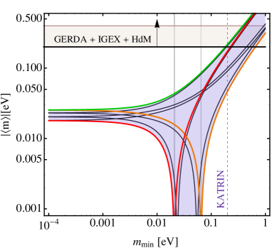
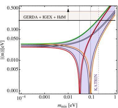
Figure 2: Left Panel. The value of $\left|\langle\!~{}m~{}\!\rangle\right|\$as a function of $m_{min}\equiv m_{1}$ in the NO case for $\Delta m^{2}_{41}=0.93\,{\rm eV^{2}}$, $\sin\theta_{14}=0.15$ and the best fit values of the oscillation parameters given in Table 1. The green, red and orange lines correspond respectively to values of the three CPV Majorana phases $(\alpha,\beta,\gamma)=(0,0,0),(0,0,\pi),(\pi,\pi,\pi)$. The five gray curves show $\left|\langle\!~{}m~{}\!\rangle\right|\$computed for the other five sets of CP conserving values of the phases. The interval between the vertical left and right solid lines, corresponding to $m_{1}=\underline{m}_{1}\simeq 0.021\,{\rm eV}$ and $m_{1}=\overline{m}_{1}\simeq 0.065\,{\rm eV}$, indicates the region where $\mbox{$\left|\langle\!~{}m~{}\!\rangle\right|\ $}_{min}=0$ for specific choices of $(\alpha,\beta,\gamma)$. Right Panel. The same as in the left panel but for $\Delta m^{2}_{41}\equiv 1.78\,{\rm eV^{2}}$. The vertical solid lines correspond to $m_{1}=\underline{m}_{1}\simeq 0.030\,{\rm eV}$ and $m_{1}=\overline{m}_{1}\simeq 0.091\,{\rm eV}$. The horizontal band indicates the upper bound $\mbox{$\left|\langle\!~{}m~{}\!\rangle\right|\ $}\sim 0.2-0.4$ eV obtained using the 90 % C.L. limit on the half-life of ⁷⁶Ge reported in [33]. See text for further details.

It proves convenient for the purposes of our analysis to work with the quantity $\mbox{$\left|\langle\!~{}m~{}\!\rangle\right|\ $}^{2}$ rather than with $\left|\langle\!~{}m~{}\!\rangle\right|\$, and to write $\mbox{$\left|\langle\!~{}m~{}\!\rangle\right|\ $}^{2}$ as

$$\mbox{$\left|\langle\!~{}m~{}\!\rangle\right|\ $}^{2}=|a+e^{i\alpha}b+e^{i\beta}c+e^{i\gamma}d|^{2}\,.$$ (9)

In the NO case under study the parameters $a$, $b$, $c$, and $d$ read:

$$\begin{split}a&=m_{min}c_{12}^{2}c_{13}^{2}c_{14}^{2}\\ b&=\sqrt{m_{min}^{2}+\Delta m^{2}_{21}}c_{13}^{2}c_{14}^{2}s_{12}^{2}\\ c&=\sqrt{m_{min}^{2}+\Delta m^{2}_{31}}c_{14}^{2}s_{13}^{2}\\ d&=\sqrt{m_{min}^{2}+\Delta m^{2}_{41}}s_{14}^{2}\,.\end{split}$$ (10)

The first derivative of $\mbox{$\left|\langle\!~{}m~{}\!\rangle\right|\ $}^{2}$ with respect of $\alpha$, $\beta$ and $\gamma$ leads to the following system of three coupled equations:

$$\begin{split}-&2b[a\sin(\alpha)+c\sin(\alpha-\beta)+d\sin(\alpha-\gamma)]=0,\\ -&2c[a\sin(\beta)-b\sin(\alpha-\beta)+d\sin(\beta-\gamma)]=0,\\ &2d[-a\sin(\gamma)+b\sin(\alpha-\gamma)+c\sin(\beta-\gamma)]=0.\\ \end{split}$$ (11)

It is possible to solve this system of equations using the set of variables $v=\tan(\alpha/2)$, $t=\tan(\beta/2)$, $u=\tan(\gamma/2)$ with $\alpha$, $\beta$, $\gamma\neq\pi+2k\pi$. We will give here only the basic formulas and will describe the results of such minimization using the best fit values given in Table 1 and eqs. (4) and (5). In Appendix A we describe in detail the minimization procedure of the general expression of $\left|\langle\!~{}m~{}\!\rangle\right|\$ in the 3+1 scheme and the 16 solutions found. We give explicit expressions for the solutions and derive the domain of each of the 16 solutions. Eight of these solutions correspond to all possible combinations of the phases having values $0$ or $\pi$. Obviously, the solution $(\alpha,\beta,\gamma)=(0,0,0)$ corresponds to an absolute maximum of the effective Majorana mass $\left|\langle\!~{}m~{}\!\rangle\right|\$. As we show in Appendix A, the domains of the solutions of interest are determined by the properties of the functions $f_{i}$, $i=1,...,8$:

$$\begin{split}f_{1}&=a-b-c-d\,,\qquad f_{2}=a+b-c-d\,,\\ f_{3}&=a+b-c+d\,,\qquad f_{4}=-a+b+c-d\,,\\ f_{5}&=a+b+c+d\,,\qquad f_{6}=a-b+c+d\,,\\ f_{7}&=a-b+c-d\,,\qquad f_{8}=a+b+c-d\,,\\ \end{split}$$ (12)

where $a$, $b$, $c$ and $d$ for the NO case are defined in eq. (10).

We will focus first on the solutions which minimize $\left|\langle\!~{}m~{}\!\rangle\right|\$ such that the minimum value is exactly zero. As is shown in Appendix A.1, there are six physical solutions for which $\mbox{$\left|\langle\!~{}m~{}\!\rangle\right|\ $}_{min}=0$: $(u_{\pm},v_{\pm},t_{\pm})$, $(u^{\pm}_{3},v^{\pm}_{3},t^{\pm}_{3})$, $(v^{\pm}_{4}(u),t^{\pm}_{4}(u))$. In order to study the domain of existence of these solutions we define the following points $\underline{m}_{1}<\hat{m}_{1}<\tilde{m}_{1}<\overline{m}_{1}$ as the zeros of the functions $f_{8}$, $f_{2}$, $f_{7}$, $f_{1}$, respectively:

$$f_{8}(\underline{m}_{1})=0,\quad f_{2}(\hat{m}_{1})=0,\quad f_{7}(\tilde{m}_{1})=0,\quad f_{1}(\overline{m}_{1})=0.$$ (13)

We find from the numerical analysis performed in Appendix A.1 that i) the solution $(u_{\pm},v_{\pm},t_{\pm})$ is valid between the zeros of the function $f_{2}$ and $f_{1}$ (the region in which $f_{1}f_{2}f_{3}f_{4}>0$), i.e. in the interval $\hat{m}_{1}<m_{1}<\overline{m}_{1}$; ii) the solution $(u^{\pm}_{3},v^{\pm}_{3},t^{\pm}_{3})$ is valid between the zeros of the function $f_{7}$ and $f_{1}$, i.e. in the interval $\tilde{m}_{1}<m_{1}<\overline{m}_{1}$; and finally iii) the solution $(v^{\pm}_{4}(u),t^{\pm}_{4}(u))$ is valid in the interval between the zero of the function $f_{8}$ and $f_{1}$, i.e. for $\underline{m}_{1}<m_{1}<\overline{m}_{1}$. In Appendix A.1 we give the numerical ranges that define the domains of the solutions discussed above. Using the best fit values of the neutrino oscillation parameters given in Table 1 and eqs. (4) and (5), we get the following numerical values of $\underline{m}_{1}$, $\hat{m}_{1}$, $\tilde{m}_{1}$, $\overline{m}_{1}$:

• for $\Delta m^{2}_{41}=0.93~{}{\rm eV^{2}}$ we have $(\underline{m}_{1},\hat{m}_{1},\tilde{m}_{1},\overline{m}_{1})\simeq(0.021,0.024,0.055,0.065)$ eV;

• if $\Delta m^{2}_{41}=1.78~{}{\rm eV^{2}}$ we get $(\underline{m}_{1},\hat{m}_{1},\tilde{m}_{1},\overline{m}_{1})\simeq(0.030,0.033,0.078,0.091)$ eV.

For $m_{1}=\underline{m}_{1}$ and $m_{1}=\overline{m}_{1}$ the value of $\left|\langle\!~{}m~{}\!\rangle\right|\$ is exactly zero for the CP conserving values of the phases $(\alpha,\beta,\gamma)=(0,0,\pi)$ and $(\pi,\pi,\pi)$, respectively. In the intervals described above (excluding the extrema), it is possible to have $\mbox{$\left|\langle\!~{}m~{}\!\rangle\right|\ $}_{min}=0$ for specific values of $(\alpha,\beta,\gamma)$, which are not necessarily CP conserving. This can be seen in Fig. 3. The numerical minima depicted in Fig. 3 are obtained minimizing $\left|\langle\!~{}m~{}\!\rangle\right|\$ by performing a scan for different values of $m_{1}$ and the CPV Majorana phases.

The grey horizontal band in Fig. 3 corresponds to $\mbox{$\left|\langle\!~{}m~{}\!\rangle\right|\ $}_{min}\leq 10^{-8}$ eV and reflects the precision of the numerical calculation of $\mbox{$\left|\langle\!~{}m~{}\!\rangle\right|\ $}_{min}=0$. The minima are reached at specific values of the phases $(\alpha,\beta,\gamma)$ that can have either CP conserving or CP nonconserving values. For $\Delta m^{2}_{41}=0.93\,{\rm eV^{2}}$ and $m_{1}=0.03\,{\rm eV}$, for instance, we have $\mbox{$\left|\langle\!~{}m~{}\!\rangle\right|\ $}=0$ if the three CPV phases have the following CP nonconserving values: $(\alpha,\beta,\gamma)=(1.731,0.023,-2.711)$. Similarly, if $\Delta m^{2}_{41}=1.78~{}{\rm eV^{2}}$ and, e.g., $m_{1}=0.04\,{\rm eV}$, we find that $\mbox{$\left|\langle\!~{}m~{}\!\rangle\right|\ $}=0$ for $(\alpha,\beta,\gamma)=(1.511,-0.365,-2.761)$.

Figure 3: Minimum $\left|\langle\!~{}m~{}\!\rangle\right|\$as function of $m_{min}\equiv m_{1}$ for $\Delta m^{2}_{41}=0.93\,{\rm eV^{2}}$ and $\sin\theta_{14}=0.15$. The plot has been obtained numerically by performing a scan over a sufficiently large sets of values of $m_{min}$ and of each of the CPV phases $(\alpha,\beta,\gamma)$ in the interval $[0,\pi]$. The black vertical lines correspond respectively to $m_{min}=\underline{m}_{1}\simeq 0.021$ eV, $m_{min}=\hat{m}_{1}\simeq 0.024$ eV and $m_{min}=\overline{m}_{1}\simeq 0.065$ eV.

Combining the results described above we can conclude that the effective Majorana mass $\left|\langle\!~{}m~{}\!\rangle\right|\$ can be zero only for values of $m_{min}$ from the following interval:

$$\underline{m}_{1}\leq m_{min}\leq\overline{m}_{1}\,\,.$$ (14)

We will derive next simple approximate analytical expressions for $\overline{m}_{1}$ and $\underline{m}_{1}$. We note first that for values of $m_{min}$ in the range $0.02-0.10$ eV, the term proportional to $\sqrt{m_{min}^{2}+\Delta m^{2}_{31}}c^{2}_{14}s^{2}_{13}$ is approximately by an order of magnitude smaller than the other three terms in $\left|\langle\!~{}m~{}\!\rangle\right|\$ (the terms with the factors $a,b,d$ in eq. (9)). Neglecting it as well as $\Delta m^{2}_{21}\ll\Delta m^{2}_{31},\Delta m^{2}_{41}$, we find the following rather simple analytic expressions for $\overline{m}_{1}$ and $\underline{m}_{1}$, which are valid up to an error of about $10\%$:

$$\begin{split}\overline{m}_{1}&\approx\sqrt{\frac{\Delta m^{2}_{41}\sin^{4}\theta_{14}}{\cos^{4}\theta_{13}\left(-\cos^{2}\theta_{12}\cos^{2}\theta_{14}+\sin^{2}\theta_{12}\right)^{2}-\sin^{4}\theta_{14}}}\,\,,\\ \underline{m}_{1}&\approx\sqrt{\frac{\Delta m^{2}_{41}\sin^{4}\theta_{14}}{\cos^{4}\theta_{13}\left(\cos^{2}\theta_{12}\cos^{2}\theta_{14}+\sin^{2}\theta_{12}\right)^{2}-\sin^{4}\theta_{14}}}\,\,.\\ \end{split}$$ (15)

Using these expressions we get $(\underline{m}_{1},\overline{m}_{1})\simeq(0.023,0.060)$ eV for $\Delta m^{2}_{41}=0.93~{}{\rm eV^{2}}$ instead of $(0.021,0.065)$ eV, and $(\underline{m}_{1},\overline{m}_{1})\simeq(0.032,0.085)$ eV for $\Delta m^{2}_{41}=1.78~{}{\rm eV^{2}}$ instead of $(0.030,0.091)$ eV.

In Fig. 2 we show two plots of $\left|\langle\!~{}m~{}\!\rangle\right|\$ as function of the lightest neutrino mass $m_{min}\equiv m_{1}$ using $\Delta m^{2}_{41}=0.93~{}{\rm eV^{2}}$ and $\Delta m^{2}_{41}=1.78~{}{\rm eV^{2}}$. The shaded area is the region of allowed values of $\left|\langle\!~{}m~{}\!\rangle\right|\$. One can see that the green curve represents the possible maximum value for $\left|\langle\!~{}m~{}\!\rangle\right|\$corresponding to $(\alpha,\beta,\gamma)=(0,0,0)$. We notice also that in the limit of $m_{min}\rightarrow 0$ the minimum value of $\mbox{$\left|\langle\!~{}m~{}\!\rangle\right|\ $}>0.01$ eV. This limit will be analyzed in detail below. We also show in Fig. 2 the prospective sensitivity to $m_{min}$ of the $\beta$-decay experiment KATRIN [34], which is under preparation.

As is well known, in the case of 3-neutrino mixing and IH (IO) neutrino mass spectrum we have $|\mbox{$\langle\!~{}m~{}\!\rangle$}^{(3\nu)}|>0.01$ eV (see, e.g., [1]). We find that in the $3+1$ scheme under discussion and NO neutrino mass spectrum we have always $\mbox{$\left|\langle\!~{}m~{}\!\rangle\right|\ $}>0.01$ eV for the following ranges of $m_{min}$:

• $m_{min}<0.010$ eV and $m_{min}>0.093$ eV, if $\Delta m^{2}_{41}=0.93~{}{\rm eV^{2}}$;

• $m_{min}<0.020$ eV and $m_{min}>0.119$ eV, for $\Delta m^{2}_{41}=1.78~{}{\rm eV^{2}}$.

What would be the changes of our results presented for $\Delta m^{2}_{41}=1.78~{}{\rm eV^{2}}$ presented so far if instead of $\sin^{2}\theta_{14}=0.023$ we used the minimal (maximal) value of the 2$\sigma$ interval (6) of allowed values $\sin^{2}\theta_{14}=0.017$ ($\sin^{2}\theta_{14}=0.047$) in the analysis? Qualitatively no new features appear and the results remain the same. Quantitatively some of the numarical values of $|<m>|$, $\overline{m}_{1}$ and $\underline{m}_{1}$, quoted in the text and obtained for $\sin^{2}\theta_{14}=0.023$, are just shifted. More specifically, this will lead to the decreasing (increasing) of the values of $|<m>|$ at $m_{min}\lesssim 10^{-3}$ eV and of $\overline{m}_{1}$ and $\underline{m}_{1}$ approximately by the same factor 1.35 (2.04).

For $0\leq m_{1}<\underline{m}_{1}$ and $m_{1}>\overline{m}_{1}$, there are no physical solutions for the phases for which $\mbox{$\left|\langle\!~{}m~{}\!\rangle\right|\ $}=0$. Moreover, $(u_{\pm},v_{\pm},t_{\pm})$, $(u^{\pm}_{3},v^{\pm}_{3},t^{\pm}_{3})$ and $(v^{\pm}_{4}(u),t^{\pm}_{4}(u))$ are not well defined in the indicated intervals. However, by studying the Hessian of $\mbox{$\left|\langle\!~{}m~{}\!\rangle\right|\ $}^{2}$, we find that there are physical solutions (among those listed in eq. (LABEL:condmin2) of Appendix A) for which $\mbox{$\left|\langle\!~{}m~{}\!\rangle\right|\ $}_{min}\neq 0$. These solutions are realised for specific values of the phases, i.e., for $(\alpha,\beta,\gamma)=(0,0,\pi)$ or $(\pi,\pi,\pi)$. The analysis performed in Appendix A allowed to find the minima of $\left|\langle\!~{}m~{}\!\rangle\right|\$at $m_{min}<\underline{m}_{1}$ for $(\alpha,\beta,\gamma)=(0,0,\pi)$, and at $m_{min}>\overline{m}_{1}$ for $(\alpha,\beta,\gamma)=(\pi,\pi,\pi)$. The domain of the solution at $m_{min}<\underline{m}_{1}$, corresponding to $(\alpha,\beta,\gamma)=(0,0,\pi)$, is the common interval of values of $m_{min}$ in which the three inequalities $c<d$, $b<d-c$ and $f_{8}=a+b+c-d<0$ hold. The domain of the solution at $m_{min}>\overline{m}_{1}$ with $(\alpha,\beta,\gamma)=(\pi,\pi,\pi)$ is determined by the inequality $f_{1}=a-b-c-d>0$. Actually, as it is possible to show, we have, in particular, $f_{8}<0$ at $m_{min}<\underline{m}_{1}$, and $f_{1}>0$ for $m_{min}>\overline{m}_{1}$.
The analysis of the Hessian of $\mbox{$\left|\langle\!~{}m~{}\!\rangle\right|\ $}^{2}$ performed in Appendix A shows that there can be two more solutions for which $\mbox{$\left|\langle\!~{}m~{}\!\rangle\right|\ $}_{min}\neq 0$. They correspond two i) $(\alpha,\beta,\gamma)=(0,\pi,0)$ and ii) $(\pi,0,0)$. The domains of these solutions (following from the Sylvester’s criterion) are determined by i) $c>d$, $b<c-d$, $-f_{3}=-a-b+c-d>0$, and ii) $b>c+d$, $-f_{6}=-a+b-c-d>0$. However, it is not difficult to convince oneself that for the values of the neutrino oscillation parameters, including those of $\Delta m^{2}_{41}$ and $\sin^{2}\theta_{14}$ used by us in the present analysis, there are no physical values of $m_{min}\geq 0$ for which the inequalities in i) or in ii) are satisfied.

In Fig. 4 we show all the relevant functions entering in the four sets of inequalities listed above (and in eq. (LABEL:condmin2) of Appendix A) which ensure that the minima $\mbox{$\left|\langle\!~{}m~{}\!\rangle\right|\ $}_{min}\neq 0$. The figure is obtained for the best fit values of the oscillation parameters given in Table 1 and for $\Delta m^{2}_{41}=0.93\,{\rm eV^{2}}$ (left panel) and $\Delta m^{2}_{41}=1.78\,{\rm eV^{2}}$ (right panel). One can easily check that only the two sets of conditions, corresponding to $(\alpha,\beta,\gamma)=(0,0,\pi)$ or $(\pi,\pi,\pi)$ and given above , are satisfied.

In Figs. 5 and 6 we show as an illustrative examples $(\tan\alpha/2,\tan\beta/2,\tan\gamma/2)$ as function of $m_{min}$ for two of the physical solutions, namely, $(u_{-},t_{-},v_{-})$ and $(v^{+}_{4},t^{+}_{4})$, found in Appendix A:

$$\begin{split}&\begin{cases}u_{\pm}&=\pm\,\sqrt{\dfrac{(-a+b+c-d)(a+b-c+d)}{(a-b-c-d)(a+b-c-d)}},\\ v_{\pm}&=\pm\,\dfrac{(b+c)}{(b-c)}\dfrac{[(a+b-c)^{2}-d^{2}]}{\sqrt{(-a+b+c-d)(a+b-c+d)(a-d-c-b)(a-d-c+b)}},\\ t_{\pm}&=\pm\,\dfrac{a^{2}+b^{2}-c^{2}-d^{2}}{\sqrt{(a-b-c-d)(a+b-c-d)(-a+b+c-d)(a+b-c+d)}},\\ \end{cases}\\ \end{split}$$ (16)

$$\begin{split}&\begin{cases}v^{\pm}_{4}(u)&=\dfrac{4bdu\pm F(a,b,c,d,u)}{-u^{2}(a-b-c-d)(a-b+c-d)-(a-b+d)^{2}+c^{2}},\\ t^{\pm}_{4}(u)&=\dfrac{-\,4cdu\pm F(a,b,c,d,u)}{u^{2}(a-b-c-d)(a+b-c-d)+(a-c+d)^{2}-b^{2}},\\ \end{cases}\\ \end{split}$$ (17)

where $a,b,c$ and $d$ are given in eq. (10) and

$$\begin{split}F(a,b,c,d,u)&=\bigg{\{}\Big{[}-u^{2}(a+b-c-d)(a-b+c-d)-(a+d)^{2}+(b-c)^{2}\Big{]}\times\\ &\times\Big{[}a^{2}\left(u^{2}+1\right)-2ad\left(u^{2}-1\right)-\left(u^{2}+1\right)(b+c-d)(b+c+d)\Big{]}\bigg{\}}^{1/2}.\\ \end{split}$$

The corresponding figures for, e.g., the solutions $(v_{+},t_{+},u_{+})$ and $(v^{-}_{4},t^{-}_{4})$ are obtained from Figs. 5 and 6 by reversing the $y-$axis.

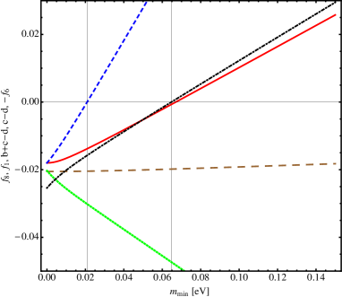
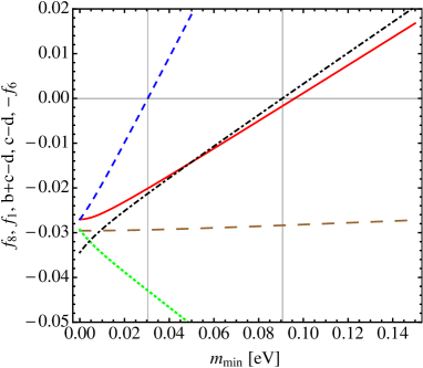
Figure 4: Left Panel. The functions $f_{8}$ (short-dashed blue), $f_{1}$ (dot-dashed black), $b+c-d$ (solid red), $c-d$ (large dashed brown), $-f_{6}$ (dotted green) versus $m_{min}\equiv m_{1}$ for $\Delta m^{2}_{41}=0.93\,{\rm eV^{2}}$ and $\sin\theta_{14}=0.15$. The vertical lines correspond to $m_{min}=\underline{m}_{1}\simeq 0.021\,{\rm eV}$ and $m_{min}=\overline{m}_{1}\simeq 0.065\,{\rm eV}$. Right Panel. The same as in the left panel, but for $\Delta m^{2}_{41}=1.78~{}{\rm eV^{2}}$. The vertical lines now are at $m_{min}=\underline{m}_{1}\simeq 0.030\,{\rm eV}$ and $m_{min}=\overline{m}_{1}\simeq 0.091\,{\rm eV}$.

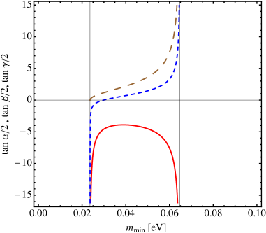
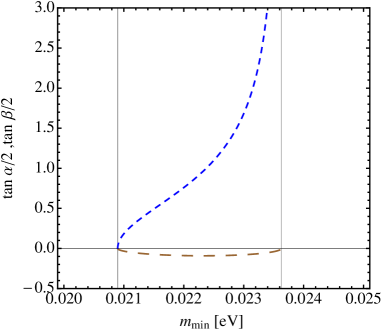
Figure 5: Left Panel. The values of $(\tan\alpha/2,\tan\beta/2,\tan\gamma/2)$ – the large dashed (brown), short dashed (blue), solid (red) lines – corresponding to the solution $(v_{-},t_{-},u_{-})$ as functions of $m_{1}$ for $\Delta m^{2}_{41}=0.93~{}{\rm eV^{2}}$. The 2nd and the 3rd vertical lines from the left are at $\hat{m}_{1}=0.024\,{\rm eV}$ and $\overline{m}_{1}=0.065\,{\rm eV}$, and indicate the domain of existence of this solution. The 1st vertical line from the left corresponds to $\underline{m}_{1}=0.021\,{\rm eV}$. Right Panel. The values of $(\tan\alpha/2,\tan\beta/2)$ – large dashed (brown), solid (red) lines – corresponding to the solution $(t^{+}_{4},v^{+}_{4})$ as functions of $m_{1}$ for $\gamma\simeq\pi$ ($u>>1$). The other parameters are the same as in the left panel. The vertical lines from the left are respectively at $\underline{m}_{1}$ and $\hat{m}_{1}$. This solution is well defined only for $\underline{m}_{1}\leq m_{1}\leq\hat{m}_{1}$.

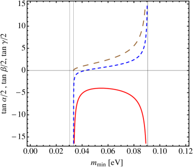
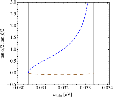
Figure 6: Left Panel. The same as in Fig. 5, left panel, for $\Delta m^{2}_{41}=1.78~{}{\rm eV^{2}}$. The 2nd and the 3rd vertical lines from the left are at $\hat{m}_{1}=0.033$ eV and $\overline{m}_{1}=0.091$ eV and indicate the domain of existence of the solution $(u_{-},t_{-},v_{-})$. The 1st vertical line from the left corresponds to $\underline{m}_{1}=0.030\,{\rm eV}$. Right Panel. The same as in Fig. 5, right panel, for $\Delta m^{2}_{41}=1.78~{}{\rm eV^{2}}$. The vertical lines from the left are at $\underline{m}_{1}$ and $\hat{m}_{1}$. The solution considered $(t^{+}_{4},v^{+}_{4})$ is well defined only in the interval $\underline{m}_{1}\leq m_{1}\leq\hat{m}_{1}$.

2.2 The Case of $m_{1}=0$

The investigation of the minima of $\left|\langle\!~{}m~{}\!\rangle\right|\$ in the NH case in the limit of $m_{1}=0$ and arbitrary values of the relevant parameters $b_{0},c_{0},d_{0}=b(m_{1}=0),c(m_{1}=0),d(m_{1}=0)$, can be done following the general analysis presented in Appendix A and, more specifically, using the system eq. (48) that can be written as

$$\begin{split}&c_{0}\sin(\alpha-\beta+\gamma-\gamma)+d_{0}\sin(\alpha-\gamma)=0\\ -&b_{0}\sin(\alpha-\beta+\gamma-\gamma)+d_{0}\sin(\beta-\gamma)=0\,,\\ \end{split}$$ (18)

with

$$b_{0}=\sqrt{\Delta m^{2}_{21}}c_{13}^{2}c_{14}^{2}s_{12}^{2}\,,\quad c_{0}=\sqrt{\Delta m^{2}_{31}}c_{14}^{2}s_{13}^{2}\,,\quad d_{0}=\sqrt{\Delta m^{2}_{41}}s_{14}^{2}\,.$$ (19)

We have solved the system eq. (18) in ($\alpha-\gamma$) and ($\beta-\gamma$) and found the solution $\sin(\alpha-\gamma)=0$, $\sin(\beta-\gamma)=0$. The solution value of $(\alpha-\gamma,\beta-\gamma)=(0,0)$ is a maximum, while the second one $(\alpha-\gamma,\beta-\gamma)=(\pi,\pi)$ is a minimum. In other words, solving the system of two equations we find a unique minimum at $(\alpha-\gamma,\beta-\gamma)=(\pi,\pi)$ independently of the value of $\Delta m^{2}_{41}$. The corresponding minimum value of $\left|\langle\!~{}m~{}\!\rangle\right|\$is 0.018 (0.027) eV in the case of $\Delta m^{2}_{41}=0.93~{}{\rm eV^{2}}~{}(1.78~{}{\rm eV^{2}})$. This result is depicted in Fig. 7. The darkest region in the figure corresponds to the minimum of $\left|\langle\!~{}m~{}\!\rangle\right|\$and the red cross indicates the precise value of ($\alpha-\gamma,\beta-\gamma$) at the minimum.

It follows from the results of our analysis that for $m_{1}=0$ and any values of the CPV phases $(\alpha-\gamma,\beta-\gamma)$ we have:

• $\mbox{$\left|\langle\!~{}m~{}\!\rangle\right|\ $}\geq 0.018\,eV$ if $\Delta m^{2}_{41}=0.93~{}{\rm eV^{2}}$;

• $\mbox{$\left|\langle\!~{}m~{}\!\rangle\right|\ $}\geq 0.027\,eV$ for $\Delta m^{2}_{41}=1.78~{}{\rm eV^{2}}$. If instead of $\sin^{2}\theta_{14}=0.0223$ we use $\sin^{2}\theta_{14}=0.017~{}(0.047)$, we get $\mbox{$\left|\langle\!~{}m~{}\!\rangle\right|\ $}\geq 0.019~{}(0.059)\,eV$.

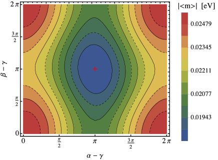
Figure 7: The value of $\left|\langle\!~{}m~{}\!\rangle\right|\$for NH spectrum in the 3+1 scheme and $m_{min}=0$. The minimum corresponds to ($\alpha-\gamma,\beta-\gamma$) =($\pi,\pi$). At the minimum (the point with the cross) $\mbox{$\left|\langle\!~{}m~{}\!\rangle\right|\ $}=1.80\times 10^{-2}\,{\rm eV}$. The values in the first four contours are, respectively, $(1.88,1.94,2.01,2.08)\times 10^{-2}\,{\rm eV}$ and obtained for $\Delta m^{2}_{41}=0.93~{}{\rm eV^{2}}$. See text for further details.

3 The case of IO Spectrum in the 3+1 Scheme

In the case of 3+1 scheme with IO 3-neutrino mass spectrum, $m_{3}<m_{1}<m_{2}<m_{4}$, one can write the effective Majorana mass following the notation in [1] as:

$$\mbox{$\left|\langle\!~{}m~{}\!\rangle\right|\ $}=|m_{1}c_{12}^{2}c_{13}^{2}c_{14}^{2}+m_{2}e^{i\alpha}c_{13}^{2}c_{14}^{2}s_{12}^{2}+m_{3}e^{i\beta}c_{14}^{2}s_{13}^{2}+m_{4}e^{i\gamma}s_{14}^{2}|\,.$$ (20)

The masses $m_{1,2,4}$ can be expressed in terms of the lightest neutrino mass $m_{min}=m_{3}$ and the neutrino mass squared differences as follows:

$$\begin{split}m_{1}=&\sqrt{m_{min}^{2}+|\Delta m^{2}_{32}|-\Delta m^{2}_{21}},\quad m_{2}=\sqrt{m_{min}^{2}+|\Delta m^{2}_{32}|},\quad m_{4}=\sqrt{m_{min}^{2}+\Delta m^{2}_{43}}\,,\\ m_{3}=&m_{min}\,,\quad\Delta m^{2}_{21}>0\,,\quad\Delta m^{2}_{32}<0\,,\quad\Delta m^{2}_{43}>0\,.\\ \end{split}$$ (21)

The neutrino mass spectrum of this scheme is depicted schematically in Fig. 8.

Figure 8: The mass spectrum in the 3+1 IO scheme.

The parameters $a$, $b$, $c$ and $d$ are given by:

$$\begin{split}a&=\sqrt{m_{min}^{2}+|\Delta m^{2}_{32}|-\Delta m^{2}_{21}}\,c_{12}^{2}c_{13}^{2}c_{14}^{2}\\ b&=\sqrt{m_{min}^{2}+|\Delta m^{2}_{32}|}\,\,c_{13}^{2}c_{14}^{2}s_{12}^{2}\\ c&=m_{min}\,\,c_{14}^{2}s_{13}^{2}\\ d&=\sqrt{m_{min}^{2}+\Delta m^{2}_{43}}\,\,s_{14}^{2}\\ \end{split}$$ (22)

In this case only a few solutions among those found in Appendix A are relevant and their existence depends on the numerical values of the parameters $a$, $b$, $c$ and $d$. In Appendix A.1 we list the domain of existence of all the solutions. Here we will analyze the solutions $(u_{\pm},v_{\pm},t_{\pm})$, given in eq. (16) with the parameters $a$, $b$, $c$ and $d$ defined in eq. (LABEL:IH31abcd), because their domain is the largest (the numerical details are given in Appendix A.1).

We observe that the solutions $(u_{\pm},v_{\pm},t_{\pm})$ are well defined when the product $f_{1}f_{2}f_{3}f_{4}$ is positive, where $f_{1,2,3,4}$ are given in eq. (12). Defining $\overline{m}_{3}$ as the zero of the function $f_{1}$, $f_{1}(\overline{m}_{3})=0$, we find that the effective Majorana mass can be zero for $m_{3}<\overline{m}_{3}$ for specific CP non-conserving values of the CPV phases $\alpha$, $\beta$ and $\gamma$. For $\Delta m^{2}_{43}=0.93~{}(1.78)~{}{\rm eV^{2}}$ and the best fit values of Table 1, we find $\overline{m}_{3}\simeq 0.038~{}(0.074)\,{\rm eV}$. These results are presented graphically in Fig. 9, where we show the numerically calculated $\mbox{$\left|\langle\!~{}m~{}\!\rangle\right|\ $}_{min}$ as function of $m_{3}$. The numerical minima depicted in Fig. 9 are obtained by performing a scan over the values of $m_{3}$ and of each of the phases $(\alpha,\beta,\gamma)$ in the interval $[0,2\pi]$. The grey horizontal band in Fig. 9, corresponding to $\mbox{$\left|\langle\!~{}m~{}\!\rangle\right|\ $}_{min}<10^{-8}$ eV, reflect the precision of the numerical calculation of $\mbox{$\left|\langle\!~{}m~{}\!\rangle\right|\ $}_{min}=0$. The minima of $\left|\langle\!~{}m~{}\!\rangle\right|\$under discussion are reached for values of the phases $(\alpha,\beta,\gamma)$ that can be either $CP$ conserving or CP non-conserving.

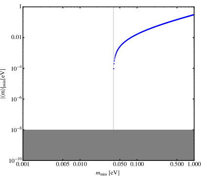
Figure 9: Minimum $\left|\langle\!~{}m~{}\!\rangle\right|\$as function of $m_{min}\equiv m_{3}$. The figure has been obtained numerically for $\Delta m^{2}_{43}=0.93\,{\rm eV^{2}}$, $\sin\theta_{14}=0.15$. The vertical line corresponds to $m_{min}=\overline{m}_{3}\simeq 0.038\,{\rm eV}$. See text for details.

We will find next an analytical approximation of $\overline{m}_{3}$. We observe that for values $m_{3}$ in the range $m_{3}\approx 0.05-0.10\,eV$ the term $\propto m_{3}\cos^{2}\theta_{14}\sin^{2}\theta_{13}$ is by approximately an order of magnitude smaller then the other three terms in $\left|\langle\!~{}m~{}\!\rangle\right|\$. Neglecting it as well the term $\propto\Delta m^{2}_{21}$, we find the following expression for $\overline{m}_{3}$, which is valid up to an error of about the $15\%$:

$$\overline{m}_{3}\approx\sqrt{\frac{\Delta m^{2}_{43}\sin^{4}\theta_{14}-\,|\Delta m^{2}_{32}|\cos^{2}2\theta_{12}\cos^{4}\theta_{13}\cos^{4}\theta_{14}}{\cos^{2}2\theta_{12}\cos^{4}\theta_{13}\cos^{4}\theta_{14}-\,\sin^{4}\theta_{14}}}\,.$$ (23)

Using this approximation we get $\overline{m}_{3}\simeq 0.032\,{\rm eV}$ for $\Delta m^{2}_{43}=0.93\,{\rm eV^{2}}$, and $\overline{m}_{3}\simeq 0.068\,{\rm eV}$ for $\Delta m^{2}_{43}=1.78\,{\rm eV^{2}}$, instead of $0.038\,{\rm eV}$ and $0.074\,{\rm eV}$ found numerically.

To find the minima of $\left|\langle\!~{}m~{}\!\rangle\right|\$for values of $m_{3}>\overline{m}_{3}$ we have to study the Hessian of $\left|\langle\!~{}m~{}\!\rangle\right|\$. From the analysis in Appendix A it follows that in the region in which $f_{1}>0$ (corresponding to the region $m_{3}>\overline{m}_{3}$), the minimum of $\left|\langle\!~{}m~{}\!\rangle\right|\$(according to the Sylvester’s criterion) takes place at $(\alpha,\beta,\gamma)=(\pi,\pi,\pi)$. In Fig. 10 we show all the relevant functions entering in the conditions determining the minima, which are listed in eq. (12) (and eq. (LABEL:condmin2)), with the parameters $a$, $b$, $c$ and $d$ defined in eq. (LABEL:IH31abcd).

In Fig. 11 we show as an example the values of the three phases versus $m_{min}$ for the solution $(u_{-},v_{-},t_{-})$. The analogous figure for the solution $(u_{+},v_{+},t_{+})$ is obtained formally from Fig. 11 by reversing the $y-$axis.

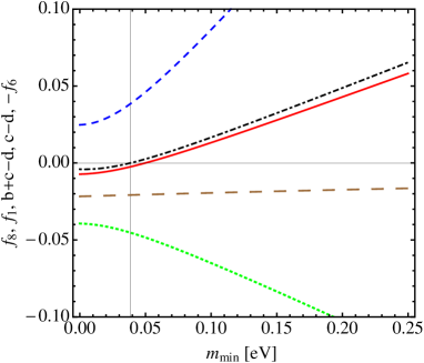
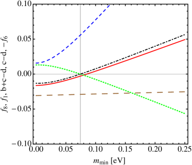
Figure 10: Left Panel. The functions $f_{8}$ (short-dashed blue), $f_{1}$ (dot-dashed black), $b+c-d$ (solid red), $c-d$ (large dashed brown), $-f_{6}$ (dotted green) versus $m_{min}\equiv m_{3}$ for $\Delta m^{2}_{43}=0.93\,{\rm eV^{2}}$, $\sin\theta_{14}=0.15$. The vertical line corresponds to $m_{min}=\overline{m}_{3}\simeq 0.038\,{\rm eV}$. Right Panel. The same as in the left panel, but for $\Delta m^{2}_{43}=1.78\,{\rm eV^{2}}$. The vertical line corresponds to $m_{min}=\overline{m}_{3}\simeq 0.074\,{\rm eV}$.

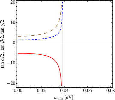
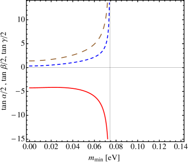
Figure 11: Left Panel. The values of $(\tan\alpha/2,\tan\beta/2,\tan\gamma/2)$ – large dashed (brown), short dashed (blue), solid (red) lines – corresponding to the solution $(v_{-},t_{-},u_{-})$, eq. (16), as functions of $m_{3}$ for $\Delta m^{2}_{43}=0.93\,{\rm eV^{2}}$, $\sin\theta_{14}=0.15$. The vertical line is at $\overline{m}_{3}=0.038\,{\rm eV}$, indicating the domain of existence of this solution, $m_{3}\leq\overline{m}_{3}$. Right Panel. The same as in the left panel, but for $\Delta m^{2}_{43}=1.78\,{\rm eV^{2}}$. The vertical line is at $\overline{m}_{3}=0.074\,{\rm eV}$, indicating the domain of existence of the solution $(v_{-},t_{-},u_{-})$, $m_{3}\leq\overline{m}_{3}$.

Finally, we show in Fig. 12 $\left|\langle\!~{}m~{}\!\rangle\right|\$as function of the lightest neutrinos mass, $m_{min}$. In this case the region of allowed values of $\left|\langle\!~{}m~{}\!\rangle\right|\$(the shaded area) is larger than in the NO case since $\left|\langle\!~{}m~{}\!\rangle\right|\$can reach zero for any $m_{min}\leq\overline{m}_{3}$. This is due to the fact that, depending on the values of the CPV phases $\alpha$, $\beta$ and $\gamma$, a complete cancellation among the terms in the expression for $\left|\langle\!~{}m~{}\!\rangle\right|\$can occur.

The results of the analysis performed in this section show that we always have $\mbox{$\left|\langle\!~{}m~{}\!\rangle\right|\ $}>0.01$ eV for:

• $m_{min}>0.078$ eV, if $\Delta m^{2}_{43}=0.93~{}{\rm eV^{2}}$;

• $m_{min}>0.108$ eV, if $\Delta m^{2}_{43}=1.78~{}{\rm eV^{2}}$.

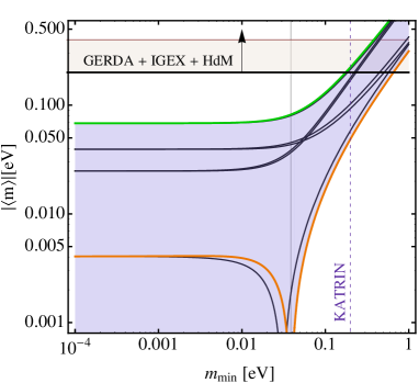
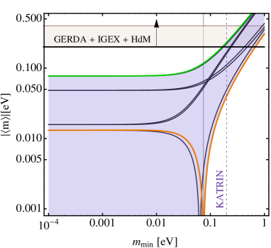
Figure 12: Left Panel. The value of $\left|\langle\!~{}m~{}\!\rangle\right|\$as function of $m_{min}=m_{3}$ for $\Delta m^{2}_{43}=0.93\,{\rm eV^{2}}$, $\sin\theta_{14}=0.15$. The green and orange lines correspond respectively to $(\alpha,\beta,\gamma)=(0,0,0)$ and $(\pi,\pi,\pi)$. The six gray curves correspond to the other possible sets of CP conserving values $0$ or $\pi$ of the CPV phases $(\alpha,\beta,\gamma)$. The vertical line is at $m_{3}=\overline{m}_{3}\simeq 0.038\,{\rm eV}$. If $m_{3}\leq\overline{m}_{3}$, we can have $\mbox{$\left|\langle\!~{}m~{}\!\rangle\right|\ $}_{min}=0$ at any fixed $m_{3}$ for specific values of $(\alpha,\beta,\gamma)$, while for $m_{3}>\overline{m}_{3}$, the minimum of $\left|\langle\!~{}m~{}\!\rangle\right|\$is realized at $(\alpha,\beta,\gamma)=(\pi,\pi,\pi)$ and $\mbox{$\left|\langle\!~{}m~{}\!\rangle\right|\ $}_{min}\neq 0$. Right Panel. The same as in the left panel, but for $\Delta m^{2}_{43}\equiv 1.78\,{\rm eV^{2}}$. The vertical line is at $m_{3}=\overline{m}_{3}\simeq 0.074\,{\rm eV}$. The horizontal band indicates the upper bound $\mbox{$\left|\langle\!~{}m~{}\!\rangle\right|\ $}\sim 0.2-0.4$ eV obtained using the 90 % C.L. limit on the half-life of ⁷⁶Ge reported in [33].

If in the case of $\Delta m^{2}_{41}=1.78~{}{\rm eV^{2}}$, instead of $\sin^{2}\theta_{14}=0.023$ we used the extreme value of the $2\sigma$ allowed interval quoted in eq. (6), $\sin^{2}\theta_{14}=0.017$ ($\sin^{2}\theta_{14}=0.047$), this will lead to the decreasing (increasing) of the numerical values of $|<m>|$ at $m_{min}\lesssim 10^{-3}$ eV and of $\overline{m}_{3}$, obtained for $\sin^{2}\theta_{14}=0.023$, approximately by the factors 1.1 (1.4) and 2.0 (2.4), respectively.

3.1 The Case of $m_{3}=0$

The effective Majorana mass in this case is

$$\mbox{$\left|\langle\!~{}m~{}\!\rangle\right|\ $}=\left|\sqrt{|\Delta m^{2}_{32}|-\Delta m^{2}_{21}}\,(c_{12}c_{13}c_{14})^{2}+\sqrt{|\Delta m^{2}_{32}|}\,(c_{13}c_{14}s_{12})^{2}e^{i\alpha}+\sqrt{\Delta m^{2}_{43}}\,s_{14}^{2}e^{i\gamma}\right|\,.$$ (24)

Now only two phases enter into the expression of $\left|\langle\!~{}m~{}\!\rangle\right|\$: $\alpha$ and $\gamma$. In this case the minima of $\left|\langle\!~{}m~{}\!\rangle\right|\$can be obtained from the general solutions derived in Appendix A and take place for

$$\begin{split}\sin\gamma_{\pm}&=\mp\frac{\sqrt{-[(a_{0}-d_{0})^{2}-b_{0}^{2}][(a_{0}+d_{0})^{2}-b_{0}^{2}]}}{2a_{0}d_{0}}\\ \sin\alpha_{\pm}&=\pm\frac{\sqrt{-[(a_{0}-d_{0})^{2}-b_{0}^{2}][(a_{0}+d_{0})^{2}-b_{0}^{2}]}}{2a_{0}b_{0}}\\ \end{split}$$ (25)

where

$$\begin{split}a_{0}&=\sqrt{|\Delta m^{2}_{32}|-\Delta m^{2}_{21}}\,\ c_{12}^{2}c_{13}^{2}c_{14}^{2}\,,\\ b_{0}&=\sqrt{|\Delta m^{2}_{32}|}\,\,c_{13}^{2}c_{14}^{2}s_{12}^{2}\,,\\ d_{0}&=\sqrt{\Delta m^{2}_{43}}\,\,s_{14}^{2}\,.\\ \end{split}$$ (26)

Both minima correspond to $\mbox{$\left|\langle\!~{}m~{}\!\rangle\right|\ $}=0$ independently of the value of $\Delta m^{2}_{43}$. However, the location of the minima on the $\alpha-\gamma$ plane depends on $\Delta m^{2}_{43}$. For instance, if we use $\Delta m^{2}_{43}=0.93~{}{\rm eV^{2}}$, the minima are at $(\sin\alpha,\sin\gamma)=(\mp 0.562,\pm 0.373)$. This result is shown in Fig. 13. We notice that the existence of solutions for $(\alpha,\gamma)$ such that $\mbox{$\left|\langle\!~{}m~{}\!\rangle\right|\ $}\sim 0$ is clear from the expression in eq. (24) since for the values of the oscillation parameters used in the present study a complete cancellation among the three terms in $\left|\langle\!~{}m~{}\!\rangle\right|\$can take place. Indeed, in the case of the best fit values, for instance,

the first term $\propto\sqrt{|\Delta m^{2}_{32}|-\Delta m^{2}_{21}}\,(c_{12}c_{13}c_{14})^{2}\approx 0.032$, can be compensated completely by the sum of the other two terms which are of the order of $\sqrt{|\Delta m^{2}_{32}|}\,(c_{13}c_{14}s_{12})^{2}\approx 0.014$ and $\sqrt{\Delta m^{2}_{43}}\,s_{14}^{2}\approx 0.022$, respectively.

It follows from our analysis that in the case of $m_{3}=0$ we have $\mbox{$\left|\langle\!~{}m~{}\!\rangle\right|\ $}>0.01$ eV for values of the phases $\alpha$ and $\gamma$ outside the region delimited by the red line in Figure 13.

We note finally that in the limit $m_{3}\rightarrow 0$ (or equivalently $c\rightarrow 0$) there are four out of the nine solutions determined analytically, which admit $\mbox{$\left|\langle\!~{}m~{}\!\rangle\right|\ $}=0$ (this can be seen in Table 5 in the Appendix A.1). The four solutions are $(u_{\pm},v_{\pm},t_{\pm})$ and $(v^{\pm}_{4}(u),t^{\pm}_{4}(u))$. If the solutions $(v^{\pm}_{4}(u),t^{\pm}_{4}(u))$ are evaluated at $u^{\pm}$, i.e., $v^{\pm}_{4}(u^{\pm})\rightarrow v_{\pm}$, in this case the two minima of the first solution coincide with the two minima of the second one.

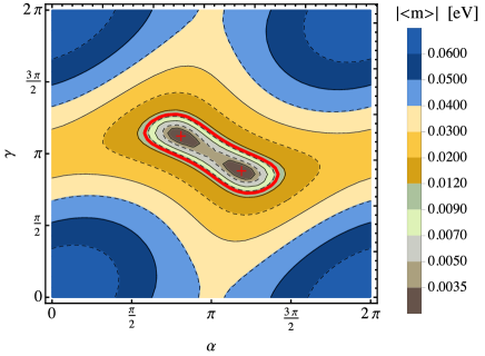
Figure 13: The values of $\left|\langle\!~{}m~{}\!\rangle\right|\$for the IH spectrum in the 3+1 scheme versus $\alpha$ and $\gamma$ in the case of $m_{min}=m_{3}=0$, $\Delta m^{2}_{43}=0.93\,{\rm eV^{2}}$ and $\sin\theta_{14}=0.15$. In this case there are two minima in the crossed points at ($\sin\alpha,\sin\gamma)=(\mp 0.562,\pm 0.373)$, and $\left|\langle\!~{}m~{}\!\rangle\right|\$in these minima is exactly zero. The red line corresponds to $\mbox{$\left|\langle\!~{}m~{}\!\rangle\right|\ $}=0.01$ eV. See text for details.

4 The 3+2 Scheme: Two Sterile Neutrinos

In this Section we analyze the case of two extra sterile neutrino states. In this case the PMNS mixing matrix is a $5\times 5$ unitary matrix. Following the parametrization used in [18] it can be written as:

$$U=V_{35}O_{34}V_{25}V_{24}O_{23}O_{15}O_{14}V_{13}V_{12}\,\,diag(1,e^{i\alpha/2},e^{i\beta/2},e^{i\gamma/2},e^{i\eta/2})\,,$$ (27)

where $\eta$ is an additional Majorana CPV phase. As in the case of the 3+1 scheme, we can set to zero the phases in the matrices $V_{25}$, $V_{24}$, $V_{13}$ and $V_{12}$ without loss of generality. In this case the elements of the first row of the PMNS matrix of interest for our analysis are given by:

$$\begin{split}U_{e1}&=c_{12}c_{13}c_{14}c_{15}\\ U_{e2}&=e^{i\alpha/2}c_{13}c_{14}c_{15}s_{12}\\ U_{e3}&=e^{i\beta/2}c_{14}c_{15}s_{13}\\ U_{e4}&=e^{i\gamma/2}c_{15}s_{14}\\ U_{e5}&=e^{i\eta/2}s_{15}\end{split}$$ (28)

The $(\beta\beta)_{0\nu}$-decay effective Majorana mass reads:

$$\mbox{$\left|\langle\!~{}m~{}\!\rangle\right|\ $}=\left|m_{1}|U_{e1}|^{2}+m_{2}|U_{e2}|^{2}e^{i\alpha}+m_{3}|U_{e3}|^{2}e^{i\beta}+m_{4}|U_{e4}|^{2}e^{i\gamma}+m_{5}|U_{e5}|^{2}e^{i\eta}\right|.$$ (29)

The values for $\theta_{14}$, $\Delta m^{2}_{41(43)}$, $\theta_{15}$ and $\Delta m^{2}_{51(53)}$ — for NO (IO)—, obtained in the global analysis performed in [18], are summarized in Table 3.

$\Delta m^{2}_{41(43)}\,\,[{\rm eV^{2}}]$	$\Delta m^{2}_{51(53)}\,\,[{\rm eV^{2}}]$	$\theta_{14}$	$\theta_{15}$
0.47	0.87	0.13	0.14

Table 3: Best global fit values of the sterile neutrino oscillation parameters in the 3+2 scheme with NO (IO) neutrino mass spectrum (from [18]). The relation to the mixing matrix elements is $|U_{e4}|=\cos\theta_{15}\sin\theta_{14}$ and $|U_{e5}|=\sin\theta_{15}$.

5 The 3+2 Scheme with NO Spectrum

In the case of the 3+2 scheme with NO spectrum, $m_{1}<m_{2}<m_{3}<m_{4}<m_{5}$, one can write the effective Majorana mass as:

$$\mbox{$\left|\langle\!~{}m~{}\!\rangle\right|\ $}=|m_{1}c_{12}^{2}c_{13}^{2}c_{14}^{2}c_{15}^{2}+m_{2}e^{i\alpha}c_{13}^{2}c_{14}^{2}c_{15}^{2}s_{12}^{2}+m_{3}e^{i\beta}c_{14}^{2}c_{15}^{2}s_{13}^{2}+m_{4}e^{i\gamma}c_{15}^{2}s_{14}^{2}+m_{5}e^{i\eta}s_{15}^{2}|\\$$ (30)

As in the case of the 3+1 scheme, it proves convenient to express the masses $m_{2,3,4,5}$ in terms of the lightest neutrino mass $m_{1}$ and the neutrino mass squared differences:

$$\begin{split}m_{min}&\equiv m_{1},\quad m_{2}=\sqrt{m_{1}^{2}+\Delta m^{2}_{21}},\quad m_{3}=\sqrt{m_{1}^{2}+\Delta m^{2}_{31}},\quad m_{4}=\sqrt{m_{1}^{2}+\Delta m^{2}_{41}},\\ m_{5}&=\sqrt{m_{1}^{2}+\Delta m^{2}_{51}},\quad\Delta m^{2}_{21}>0,\ \ \Delta m^{2}_{31}>0,\ \ \Delta m^{2}_{41}>0\,\,\,\mbox{and}\,\,\,\Delta m^{2}_{51}>0\,\,.\\ \end{split}$$ (31)

The neutrino mass spectrum in 3+2 NO scheme is shown in Fig. 14.

Figure 14: The neutrino mass spectrum in the 3+2 NO scheme.

In what follows we will analyze the conditions for minimization of $\left|\langle\!~{}m~{}\!\rangle\right|\$. As in the 3+1 case, we will work with $\mbox{$\left|\langle\!~{}m~{}\!\rangle\right|\ $}^{2}$ rather than with $\left|\langle\!~{}m~{}\!\rangle\right|\$:

$$\mbox{$\left|\langle\!~{}m~{}\!\rangle\right|\ $}^{2}=|a+e^{i\alpha}b+e^{i\beta}c+e^{i\gamma}d+e^{i\eta}e|^{2}\,,$$ (32)

where

$$\begin{split}a&=m_{min}c_{12}^{2}c_{13}^{2}c_{14}^{2}c_{15}^{2}\,,\\ b&=\sqrt{m_{min}^{2}+\Delta m^{2}_{21}}c_{13}^{2}c_{14}^{2}c_{15}^{2}s_{12}^{2}\,,\\ c&=\sqrt{m_{min}^{2}+\Delta m^{2}_{31}}c_{14}^{2}c_{15}^{2}s_{13}^{2}\,,\\ d&=\sqrt{m_{min}^{2}+\Delta m^{2}_{41}}c_{15}^{2}s_{14}^{2}\,,\\ e&=\sqrt{m_{min}^{2}+\Delta m^{2}_{51}}s_{15}^{2}\,.\\ \end{split}$$ (33)

The analytical study of the minima of $\mbox{$\left|\langle\!~{}m~{}\!\rangle\right|\ $}^{2}$ in this case is a non-trivial task since four phases are involved and the non-linearity of the system of the first derivatives of $\mbox{$\left|\langle\!~{}m~{}\!\rangle\right|\ $}^{2}$ with respect to the four phases makes the analysis rather complicated. Therefore finding all possible solutions of the minimization procedure in analytical form is a complex problem. Thus, we have performed the general analysis of the minimization of $\left|\langle\!~{}m~{}\!\rangle\right|\$numerically. It is possible, however, to perform analytically the analysis of the minima of $\left|\langle\!~{}m~{}\!\rangle\right|\$, corresponding to the 16 sets of CP conserving values (either $0$ or $\pi$) of the four phases $\alpha$, $\beta$, $\gamma$ and $\eta$. This analysis is described in Appendix B. It follows from the results found in Appendix B that only $(\alpha,\beta,\gamma,\eta)=(\pi,\pi,\pi,\pi)$, $(0,0,0,\pi)$, $(0,0,\pi,0)$, $(0,\pi,0,0)$ and $(\pi,0,0,0)$ can correspond to minima of $\left|\langle\!~{}m~{}\!\rangle\right|\$. These minima take place in intervals of values of $m_{1}$ which are determined by the following sets of inequalities:

$$\begin{split}(\alpha,\beta,\gamma,\eta)&=(\pi,\pi,\pi,\pi)\quad if\quad F_{1}=a-b-c-d-e>0,\\ (\alpha,\beta,\gamma,\eta)&=(0,0,0,\pi)\quad if\quad(d<e)\land(c<e-d)\land(b<-c-d+e)\land\\ &\phantom{,aaaaaaaaaaaaaaa}\land(F_{8}=a+b+c+d-e<0),\\ (\alpha,\beta,\gamma,\eta)&=(0,0,\pi,0)\quad if\quad(d>e)\land(c<d-e)\land(b<-c+d-e)\land\\ &\phantom{,aaaaaaaaaaaaaaa}\land(F_{3}=a+b+c-d+e<0),\\ (\alpha,\beta,\gamma,\eta)&=(0,\pi,0,0)\quad if\quad(c>d+e)\land(b<c-d-e)\land\\ &\phantom{,aaaaaaaaaaaaaaa}\land(G_{3}=a+b-c+d+e<0),\\ (\alpha,\beta,\gamma,\eta)&=(\pi,0,0,0)\quad if\quad(b>c+d+e)\land(F_{6}=a-b+c+d+e<0)\,.\end{split}$$ (34)

The dependence of $F_{1}$, $F_{8}$, $F_{3}$, $G_{3}$, $F_{6}$ and $(d-e)$ on $m_{1}$ is shown in the right panel of Fig. 15.

It is not difficult to check that for the values of the oscillation parameters quoted in Tables 1 and 3, the sets of inequalities listed above in each of the cases of $(\alpha,\beta,\gamma,\eta)=(0,0,\pi,0)$, $(0,\pi,0,0)$ and $(\pi,0,0,0)$ cannot simultaneously be fulfilled for $m_{1}\geq 0$. Thus, only $(\alpha,\beta,\gamma,\eta)=(\pi,\pi,\pi,\pi)$ and $(0,0,0,\pi)$ correspond to true minima of $\left|\langle\!~{}m~{}\!\rangle\right|\$. Defining $\overline{m}_{1}$ and $\underline{m}_{1}$ as the zero of the functions $F_{1}$ and $F_{8}$,

$$F_{1}(\overline{m}_{1})=a-b-c-d-e=0,\qquad F_{8}(\underline{m}_{1})=a+b+c+d-e=0\,,$$ (35)

we find that the minima of $\left|\langle\!~{}m~{}\!\rangle\right|\$for $m_{1}>\overline{m}_{1}$ take place only at $(\alpha,\beta,\gamma,\eta)=(\pi,\pi,\pi,\pi)$, while for $m_{1}<\underline{m}_{1}$ they occur at $(\alpha,\beta,\gamma,\eta)=(0,0,0,\pi)$. Further, the numerical analysis performed by us shows that in the interval of $\overline{m}_{1}<m_{min}<\underline{m}_{1}$, the minimum value of $\left|\langle\!~{}m~{}\!\rangle\right|\$is exactly zero and is reached, in general, for CP nonconserving values of the phases $(\alpha,\beta,\gamma,\eta)$. These results are presented graphically in the left panel of Fig. 15. Figure 15 shows also, in particular, that at $m_{min}\rightarrow 0$ we have $\mbox{$\left|\langle\!~{}m~{}\!\rangle\right|\ $}\neq 0$.

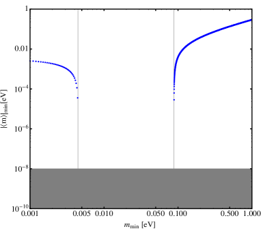
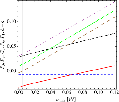
Figure 15: Left Panel. Minimum $\left|\langle\!~{}m~{}\!\rangle\right|\$as function of $m_{min}\equiv m_{1}$. The figure has been obtained numerically for $\Delta m^{2}_{41}=0.47\,{\rm eV^{2}}$, $\Delta m^{2}_{51}=0.87\,{\rm eV^{2}}$, $\sin\theta_{14}=0.13$, $\sin\theta_{15}=0.14$ (see Table 3) and performing a scan over a sufficiently large sets of values of $m_{min}$. The vertical lines correspond to $\overline{m}_{1}\simeq 8.84\times 10^{-2}$ eV and $\underline{m}_{1}\simeq 4.44\times 10^{-3}$ eV. In the interval $\underline{m}_{1}\leq m_{1}\leq\overline{m}_{1}$ we have min($\left|\langle\!~{}m~{}\!\rangle\right|\$) = 0. Right Panel. The functions $F_{3}$ (dotted green), $F_{8}$ (large dashed brown), $G_{3}$ (short-large dashed purple), $F_{6}$ (dot-dashed black), $F_{1}$ (solid red), $d-e$ (short-dashed blue), defined in eq. (35) as function of $m_{min}$ for the best fit values of Table 3. The vertical lines are at $\overline{m}_{1}\simeq 8.84\times 10^{-2}$ eV and $\underline{m}_{1}\simeq 4.44\times 10^{-3}$ eV.

In Fig. 16 we show $\left|\langle\!~{}m~{}\!\rangle\right|\$as a function of the lightest neutrino mass $m_{min}$. The shaded area indicates the allowed values for $\left|\langle\!~{}m~{}\!\rangle\right|\$. The red, orange, green and gray lines correspond to the different sets of CP conserving values (0 or $\pi$) of the CPV phases $(\alpha,\beta,\gamma)$. The vertical solid lines are at $m_{1}=\underline{m}_{1}\simeq 4.44\times 10^{-3}\,{\rm eV}$ (and $(\alpha,\beta,\gamma,\eta)=(0,0,0,\pi)$) and $m_{1}=\overline{m}_{1}\simeq 8.84\times 10^{-2}\,{\rm eV}$ (and $(\alpha,\beta,\gamma,\eta)=(\pi,\pi,\pi,\pi)$). It is clear from the figure that $\left|\langle\!~{}m~{}\!\rangle\right|\$can be zero in the interval $\underline{m}_{1}\leq m_{min}\leq\overline{m}_{1}$, while for $m_{min}\rightarrow 0$ we have $\mbox{$\left|\langle\!~{}m~{}\!\rangle\right|\ $}_{min}\rightarrow 3.21\times 10^{-3}$ eV and ${\rm max}(\mbox{$\left|\langle\!~{}m~{}\!\rangle\right|\ $})=0.033$ eV. The indicated $\mbox{$\left|\langle\!~{}m~{}\!\rangle\right|\ $}_{min}$ and ${\rm max}(\mbox{$\left|\langle\!~{}m~{}\!\rangle\right|\ $})$ values at $m_{min}=0$ in Fig. 16 are reached for $(\alpha,\beta,\gamma,\eta)=(0,0,0,\pi)$ and $(\alpha,\beta,\gamma,\eta)=(0,0,0,0)$ (corresponding to the red and green lines). At $m_{1}=\overline{m}_{1}$ and $m_{1}=\underline{m}_{1}$, we have $\mbox{$\left|\langle\!~{}m~{}\!\rangle\right|\ $}_{min}=0$: at $m_{1}=\underline{m}_{1}$ the first four terms in the expression for $\left|\langle\!~{}m~{}\!\rangle\right|\$are positive and their sum is compensated by the last term, $\sqrt{\Delta m^{2}_{51}}\sin^{2}\theta_{15}$, while at $m_{1}=\overline{m}_{1}$ a cancellation occurs between the first term proportional to $m_{min}$ and the sum of all the other terms. We have also indicated in the figure with a dotted vertical line the prospective constraint on $m_{min}$ that might be obtained in the $\beta$-decay experiment KATRIN [34]. We find that in 3+2 NO scheme under discussion one always has

• $\mbox{$\left|\langle\!~{}m~{}\!\rangle\right|\ $}>0.01$ eV for $m_{min}>0.118$ eV.

Figure 16: The value of $\left|\langle\!~{}m~{}\!\rangle\right|\$versus the lightest neutrino mass $m_{1}$ for $\Delta m^{2}_{41}=0.47\,{\rm eV^{2}}$, $\Delta m^{2}_{51}=0.87\,{\rm eV^{2}}$, $\sin\theta_{14}=0.13$, $\sin\theta_{15}=0.14$. The green, red and orange lines correspond to $(\alpha,\beta,\gamma,\eta)=(0,0,0,0),(0,0,0,\pi),(\pi,\pi,\pi,\pi)$, while the blue lines are obtained for the other 13 sets of CP conserving values (0 or $\pi$) of the four CPV phases. The vertical solid lines are at $m_{1}=\underline{m}_{1}\simeq 0.004\,{\rm eV}$ and $m_{1}=\overline{m}_{1}\simeq 0.088\,{\rm eV}$. The minimum of $\left|\langle\!~{}m~{}\!\rangle\right|\$in the interval $\underline{m}_{1}\leq m_{1}\leq\overline{m}_{1}$ is exactly zero. The horizontal band indicates the upper bound $\mbox{$\left|\langle\!~{}m~{}\!\rangle\right|\ $}\sim 0.2-0.4$ eV obtained using the 90 % C.L. limit on the half-life of ⁷⁶Ge reported in [33]. See text for further details.

5.1 The Case of $m_{1}=0$

In the case of $m_{min}\equiv m_{1}=0$, the expression of $\left|\langle\!~{}m~{}\!\rangle\right|\$symplifies to:

$$\mbox{$\left|\langle\!~{}m~{}\!\rangle\right|\ $}^{2}\bigg{|}_{m_{1}=0}=|e^{i\alpha}b_{0}+e^{i\beta}c_{0}+e^{i\gamma}d_{0}+e^{i\eta}e_{0}|^{2}\,\,,$$ (36)

where the parameters $b_{0},c_{0},d_{0}$ and $e_{0}$ read:

$$\begin{split}b_{0}&=\sqrt{\Delta m^{2}_{21}}c_{13}^{2}c_{14}^{2}s_{12}^{2}\,,\\ c_{0}&=\sqrt{\Delta m^{2}_{31}}c_{14}^{2}c_{15}^{2}s_{13}^{2}\,,\\ d_{0}&=\sqrt{\Delta m^{2}_{41}}c_{15}^{2}s_{14}^{2}\,,\\ e_{0}&=\sqrt{\Delta m^{2}_{51}}s_{15}^{2}\,.\\ \end{split}$$ (37)

The minimum of the effective Majorana mass is reached in this case for $(\alpha,\beta,\gamma,\eta)=(0,0,0,\pi)$ and at the minimum $\mbox{$\left|\langle\!~{}m~{}\!\rangle\right|\ $}\neq 0$. Indeed, numerically we have $b_{0}\simeq 2.51\times 10^{-3}$ eV, $c_{0}\simeq 1.14\times 10^{-3}$ eV, $d_{0}\simeq 1.13\times 10^{-2}$ eV and $e_{0}\simeq 1.82\times 10^{-2}$ eV, and it is clear that the four terms in the expression for $\left|\langle\!~{}m~{}\!\rangle\right|\$cannot compensate each other completely. For the minimum value of $\left|\langle\!~{}m~{}\!\rangle\right|\$in the case under study we get $\mbox{$\left|\langle\!~{}m~{}\!\rangle\right|\ $}=0.0032$ eV. In Fig. 17 we show the values of $\left|\langle\!~{}m~{}\!\rangle\right|\$versus $\alpha-\eta$ and $\beta-\eta$, fixing for convenience $\gamma-\eta=\pi$. The minimum is at the crossed point corresponding to at $\alpha-\eta=\pi$, $\beta-\eta=\pi$.

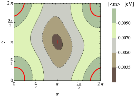
Figure 17: The value of $\left|\langle\!~{}m~{}\!\rangle\right|\$in the 3+2 scheme with NO spectrum at $m_{min}=0$ for $\gamma-\eta=\pi$. The minimum of $\left|\langle\!~{}m~{}\!\rangle\right|\$corresponds to ($\alpha-\eta,\beta-\eta$) =($\pi,\pi$) (the crossed point). The values of $\left|\langle\!~{}m~{}\!\rangle\right|\$at this minimum is $3.21\,\times 10^{-3}$ eV. The red line corresponds to $\mbox{$\left|\langle\!~{}m~{}\!\rangle\right|\ $}=0.01$ eV.

It follows from our analysis that in the case of $m_{1}=0$ and $\gamma-\eta=\pi$ we have $\mbox{$\left|\langle\!~{}m~{}\!\rangle\right|\ $}>0.01$ eV for values of the phases $\alpha-\eta$ and $\beta-\eta$ in the region delimited by the red lines in Figure 17.

6 The 3+2 Scheme with IO Spectrum

In the case of the 3+2 scheme with IO spectrum, $m_{3}<m_{1}<m_{2}<m_{4}<m_{5}$, $\left|\langle\!~{}m~{}\!\rangle\right|\$can be written as:

$$\mbox{$\left|\langle\!~{}m~{}\!\rangle\right|\ $}=|m_{1}c_{12}^{2}c_{13}^{2}c_{14}^{2}c_{15}^{2}+m_{2}e^{i\alpha}c_{13}^{2}c_{14}^{2}c_{15}^{2}s_{12}^{2}+m_{3}e^{i\beta}c_{14}^{2}c_{15}^{2}s_{13}^{2}+m_{4}e^{i\gamma}c_{15}^{2}s_{14}^{2}+m_{5}e^{i\eta}s_{15}^{2}|\,.\\$$ (38)

We have:

$$\begin{split}m_{1}&=\sqrt{m_{3}^{2}-\Delta m^{2}_{32}-\Delta m^{2}_{21}},\quad m_{2}=\sqrt{m_{3}^{2}-\Delta m^{2}_{32}},\quad m_{3}\equiv m_{min},\quad m_{4}=\sqrt{m_{3}^{2}+\Delta m^{2}_{43}},\\ m_{5}&=\sqrt{m_{3}^{2}+\Delta m^{2}_{53}},\quad\Delta m^{2}_{21}>0\,,\ \ \Delta m^{2}_{32}<0\,,\ \ \Delta m^{2}_{43}>0\,,\qquad\Delta m^{2}_{53}>0\,.\\ \end{split}$$ (39)

The neutrino mass spectrum in 3+2 IO scheme is shown schematically in Fig. 18.

Figure 18: The neutrino mass spectrum in the 3+2 IO scheme.

We define:

$$\mbox{$\left|\langle\!~{}m~{}\!\rangle\right|\ $}^{2}=|a+e^{i\alpha}b+e^{i\beta}c+e^{i\gamma}d+e^{i\eta}e|^{2}\,\,,$$ (40)

where the parameters $a$, $b$, $c$, $d$ and $e$ in this case read:

$$\begin{split}a&=\sqrt{m_{min}^{2}+|\Delta m^{2}_{32}|-\Delta m^{2}_{21}}c_{12}^{2}c_{13}^{2}c_{14}^{2}c_{15}^{2}\,,\\ b&=\sqrt{m_{min}^{2}+|\Delta m^{2}_{32}|}c_{13}^{2}c_{14}^{2}c_{15}^{2}s_{12}^{2}\,,\\ c&=m_{min}c_{14}^{2}c_{15}^{2}s_{13}^{2}\,,\\ d&=\sqrt{m_{min}^{2}+\Delta m^{2}_{43}}c_{15}^{2}s_{14}^{2}\,,\\ e&=\sqrt{m_{min}^{2}+\Delta m^{2}_{53}}s_{15}^{2}\,.\\ \end{split}$$ (41)

As in the case of NO spectrum, we have performed the general analysis of minimization of $\left|\langle\!~{}m~{}\!\rangle\right|\$ numerically. Analytical results have been obtained only for the CP conserving values (0 or $\pi$) of the four CPV phases. As it follows from the analysis performed in Appendix B, only one set of CP conserving values of the phases corresponds to a minimum of $\left|\langle\!~{}m~{}\!\rangle\right|\$, namely, $(\alpha,\beta,\gamma,\eta)=(\pi,\pi,\pi,\pi)$. The domain of this minimization solution is determined by the inequality $F_{1}(m_{3})\equiv(a-b-c-d-e)>0$. Let us define by $\overline{m}_{3}$ the zero of $F_{1}$: $F_{1}(\overline{m}_{3})=0$. As can be shown (and is seen also in Fig. 22 in Appendix B), the inequality of interest $F_{1}(m_{3})>0$ is satisfied for $m_{3}>\overline{m}_{3}$. Thus, for $m_{3}>\overline{m}_{3}$, $\left|\langle\!~{}m~{}\!\rangle\right|\$takes minimum values only for the values of the phases $(\alpha,\beta,\gamma,\eta)=(\pi,\pi,\pi,\pi)$. Moreover, the minima of $\left|\langle\!~{}m~{}\!\rangle\right|\$at $m_{3}>\overline{m}_{3}$ are different from zero. This follows from the fact that the minima under discussion correspond to the contribution of the first term $\propto\sqrt{m_{min}^{2}+|\Delta m^{2}_{32}|-\Delta m^{2}_{21}}$ in the expression for $\left|\langle\!~{}m~{}\!\rangle\right|\$, eq. (38), being compensated by the sum of the other terms in $\left|\langle\!~{}m~{}\!\rangle\right|\$, and that for the values of the oscillation parameters used in the present analysis the compensation cannot be complete. For the indicated values of the phases, a complete compensation leading to $\mbox{$\left|\langle\!~{}m~{}\!\rangle\right|\ $}_{min}=0$ is possible only in the point $m_{3}=\overline{m}_{3}$. At any given $m_{3}<\overline{m}_{3}$, as our numerical analysis shows, we have $\mbox{$\left|\langle\!~{}m~{}\!\rangle\right|\ $}_{min}=0$ and the minimum takes place, in general, for CP nonconserving values of $(\alpha,\beta,\gamma,\eta)$. These results are illustrated in Fig. 19, where we show $\mbox{$\left|\langle\!~{}m~{}\!\rangle\right|\ $}_{min}$ as function of the lightest neutrino mass.

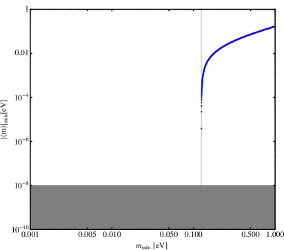
Figure 19: Minimum $\left|\langle\!~{}m~{}\!\rangle\right|\$as a function of $m_{min}\equiv m_{3}$. The plot has been obtained numerically for $\Delta m^{2}_{43}=0.47\,{\rm eV^{2}}$, $\Delta m^{2}_{53}=0.87\,{\rm eV^{2}}$, $\sin\theta_{14}=0.13$, $\sin\theta_{15}=0.14$ (see Table 3) by varying $m_{min}$ in the interval [0.001, 1.000] eV and each of the four CPV phases in the interval $[0,2\pi]$. The vertical line corresponds to $\overline{m}_{3}\simeq 1.25\times 10^{-1}$ eV ($F_{1}(\overline{m}_{3})=0$). For any given $m_{3}\leq\overline{m}_{3}$ we have $\mbox{$\left|\langle\!~{}m~{}\!\rangle\right|\ $}_{min}=0$. For the different $m_{3}<\overline{m}_{3}$, the minima of $\left|\langle\!~{}m~{}\!\rangle\right|\$occur at different sets of CP nonconserving values of $(\alpha,\beta,\gamma,\eta)$ (see text for further details).

In Fig. 20 we show $\left|\langle\!~{}m~{}\!\rangle\right|\$as function of the lightest neutrino mass $m_{min}=m_{3}$. The gray lines correspond to $\left|\langle\!~{}m~{}\!\rangle\right|\$computed for $CP$ conserving values of the phases $(\alpha,\beta,\gamma,\eta)$ (either 0 or $\pi$). The shaded area indicates the possible allowed values of $\left|\langle\!~{}m~{}\!\rangle\right|\$and is obtained for the values of the oscillation parameters quoted in Tables 1 and 3. The vertical solid line corresponds to $m_{min}=\overline{m}_{3}\simeq 0.125$ eV and $(\alpha,\beta,\gamma,\eta)=(\pi,\pi,\pi,\pi)$. At $m_{min}\leq\overline{m}_{3}$, we can have $\mbox{$\left|\langle\!~{}m~{}\!\rangle\right|\ $}_{min}=0$ for specific, in general CP nonconserving, values of the phases $(\alpha,\beta,\gamma,\eta)$. This behaviour of $\mbox{$\left|\langle\!~{}m~{}\!\rangle\right|\ $}_{min}$ is very different from the behavior in the case of NO spectrum discussed in the previous Section, where $\mbox{$\left|\langle\!~{}m~{}\!\rangle\right|\ $}_{min}$ can be zero only in a limited interval of values of $m_{min}$.

We find also that in the 3+2 IO scheme under discussion and the values of the neutrino oscillation parameters used in the present analysis one always has

• $\mbox{$\left|\langle\!~{}m~{}\!\rangle\right|\ $}>0.01$ eV for $m_{min}>0.178$ eV.

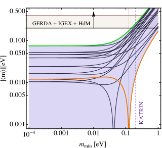
Figure 20: The value of $\left|\langle\!~{}m~{}\!\rangle\right|\$as function of $m_{min}=m_{3}$ for $\Delta m^{2}_{43}=0.47~{}{\rm eV^{2}}$, $\Delta m^{2}_{53}=0.87~{}{\rm eV^{2}}$, $\sin\theta_{14}=0.13$, $\sin\theta_{15}=0.14$ (see Table 3). The green and orange lines correspond to $(\alpha,\beta,\gamma)=(0,0,0,0)$ and $(\pi,\pi,\pi,\pi)$, while the gray lines corresponding to the other 14 sets of CP conserving values (0 or $\pi$) of the four CPV phases. The vertical solid line corresponds to $m_{min}=\overline{m}_{3}\simeq 0.125$ eV. At $m_{min}\leq\overline{m}_{3}$ we can have $\mbox{$\left|\langle\!~{}m~{}\!\rangle\right|\ $}_{min}=0$. The dotted line represents the prospective upper limit from the $\beta$-decay experiment KATRIN [34]. The horizontal band indicates the upper bound $\mbox{$\left|\langle\!~{}m~{}\!\rangle\right|\ $}\sim 0.2-0.4$ eV obtained using the 90 % C.L. limit on the half-life of ⁷⁶Ge given in [33].

6.1 The case of $m_{3}=0$

In the limit $m_{min}\equiv m_{3}=0$, (which implies $c=0$ in eq. (40)), the analysis of the minimization of the effective Majorana mass is exactly the same as in the case of the 3+1 scheme. This becomes clear after a redefinition of the phases and the coefficients involved. For $m_{min}\equiv m_{3}=0$, $\mbox{$\left|\langle\!~{}m~{}\!\rangle\right|\ $}^{2}$ can be written as:

$$\mbox{$\left|\langle\!~{}m~{}\!\rangle\right|\ $}^{2}\bigg{|}_{m_{3}=0}=|a_{0}+e^{i\alpha}b_{0}+e^{i\gamma}d_{0}+e^{i\eta}e_{0}|^{2}\,\,,$$ (42)

where

$$\begin{split}a_{0}&=\sqrt{|\Delta m^{2}_{32}|-\Delta m^{2}_{21}}\,c_{12}^{2}c_{13}^{2}c_{14}^{2}c_{15}^{2}\,,\\ b_{0}&=\sqrt{|\Delta m^{2}_{32}|}\,c_{13}^{2}c_{14}^{2}c_{15}^{2}s_{12}^{2}\,,\\ d_{0}&=\sqrt{\Delta m^{2}_{43}}\,c_{15}^{2}s_{14}^{2}\,,\\ e_{0}&=\sqrt{\Delta m^{2}_{53}}\,s_{15}^{2}\,.\\ \end{split}$$ (43)

Using the analysis performed in Appendix A for the 3+1 scheme we find that the solutions which minimize $\left|\langle\!~{}m~{}\!\rangle\right|\$, such that $\mbox{$\left|\langle\!~{}m~{}\!\rangle\right|\ $}_{min}$ is exactly zero, are: $(u_{\pm},v_{\pm},t_{\pm})$$\equiv$ $(\tan(\gamma_{\pm}/2),$ $\tan(\alpha_{\pm}/2),$ $\tan(\eta_{\pm}/2))$, $(u^{\pm}_{3},v^{\pm}_{3},t^{\pm}_{3})$ $\equiv$ $(\tan(\gamma^{\pm}_{3}/2),\tan(\alpha^{\pm}_{3}/2),\tan(\eta^{\pm}_{3}/2))$, and $(v^{\pm}_{4}(u),t^{\pm}_{4}(u))\equiv(\tan(\alpha^{\pm}_{4}/2),\tan(\eta^{\pm}_{4}/2))$. The solutions $(u_{\pm},v_{\pm},t_{\pm})$ and $(v^{\pm}_{4}(u),t^{\pm}_{4}(u))$ can be obtained formally from eqs. (16) and (17) by replacing, respectively, $a$, $b$, $c$ and $d$ with $a_{0}$, $b_{0}$, $e_{0}$ and $d_{0}$ defined in eq. (43), while the solution $(u^{\pm}_{3},v^{\pm}_{3},t^{\pm}_{3})$ is given by:

$$\begin{split}\begin{cases}u^{\pm}_{3}&=\pm\dfrac{\sqrt{(-a_{0}+b_{0}-d_{0}+e_{0})(a_{0}-b_{0}+d_{0}+e_{0})}}{\sqrt{(a_{0}-b_{0}-d_{0}-e_{0})(a_{0}-b_{0}-d_{0}+e_{0})}}\,,\\ v^{\pm}_{3}&=\pm\dfrac{a_{0}^{2}-b_{0}^{2}-d_{0}^{2}+e_{0}^{2}}{\sqrt{(a_{0}-b_{0}-d_{0}-e_{0})(a_{0}-b_{0}-d_{0}+e_{0})}\sqrt{(-a_{0}+b_{0}-d_{0}+e_{0})(a_{0}-b_{0}+d_{0}+e_{0})}}\,,\\ t^{\pm}_{3}&=\pm\dfrac{(b_{0}+e_{0})(-a_{0}+b_{0}+d_{0}-e_{0})\sqrt{(-a_{0}+b_{0}-d_{0}+e_{0})(a_{0}-b_{0}+d_{0}+e_{0})}}{(b_{0}-e_{0})\sqrt{(a_{0}-b_{0}-d_{0}-e_{0})(a_{0}-b_{0}-d_{0}+e_{0})}(-a_{0}+b_{0}-d_{0}+e_{0})}\,.\\ \end{cases}\end{split}$$ (44)

Using the best fit values $\Delta m^{2}_{43}=0.47\,{\rm eV^{2}}$, $\Delta m^{2}_{53}=0.87\,{\rm eV^{2}}$, $\sin\theta_{14}=0.13$, $\sin\theta_{15}=0.14$ we find that the minima corresponding to $(u_{\pm},v_{\pm},t_{\pm})$ and to eq. (44) are given numerically by:

$$u_{\pm}\simeq\pm 1.44,\quad v_{\pm}\simeq\pm 18.5,\quad t_{\pm}\simeq\mp 2.61$$ (45)

and

$$u^{\pm}_{3}\simeq\pm 1.30,\quad v^{\pm}_{3}\simeq\mp 2.63,\quad t^{\pm}_{3}\simeq\mp 24.7\,.$$ (46)

The third minimum corresponding to the solution $(v^{\pm}_{4}(u),t^{\pm}_{4}(u))$ is not determined uniquely since it depends on $u$. However, one can define the minimum for a specific choice of $u$, or equivalently, for a value for one of the other phases, because the expressions of this solution are invertible. In order to check numerically whether the three solutions are minima we plot the dependence of $\left|\langle\!~{}m~{}\!\rangle\right|\$on two of the CPV phases $(\alpha,\gamma,\eta)$, fixing the value of the third phase. It proves convenient to set the value of $\eta$, i.e. of $t$, equal to the values of the solution $(u_{\pm},v_{\pm},t_{\pm})$. One can, of course, do the same using the solutions $(u^{\pm}_{3},v^{\pm}_{3},t^{\pm}_{3})$, or choosing an arbitrary value of $\eta$. Our aim is to show that in the 3+2 IO scheme with $m_{3}=0$, the two solutions $(u^{+},v^{+},t^{+})$ and $(v^{+}_{4}(u),t^{+}_{4}(u))$ represent two different minima, in contrast to the case of 3+1 IO scheme with $m_{3}=0$.

More specifically, if we fix $t\simeq-2.61$, we find $v^{+}_{4}\simeq 1.68$ at a value of $u^{+}_{4}\simeq-59.3$. The Left Panel of Fig. 21 shows the values of $\left|\langle\!~{}m~{}\!\rangle\right|\$with $t=t_{+}\simeq-2.61$. The marked points correspond to the two different minima: the first corresponds to the solution $(u_{+},v_{+},t_{+})$ and takes place at $(\alpha,\gamma)=(3.03,1.93)$, while the second one is associated with the solution $(v^{+}_{4}(u),t^{+}_{4}(u))$ and occurs at $(\alpha,\gamma)=(2.07,3.17)$. In these two minima the effective Majorana mass is exactly zero. Repeating the same analysis with $t\simeq 2.61$, we find $v^{-}_{4}\simeq-1.68$ at the value of $u^{-}_{4}\simeq 59.3$. The Right Panel of Fig. 21 shows the values of $\left|\langle\!~{}m~{}\!\rangle\right|\$ with $t=t_{-}\simeq 2.61$. The points marked with a cross correspond to the two different minima, one evaluated from the function $(u_{-},v_{-},t_{-})$ and corresponding to $(\alpha,\gamma)=(3.25,4.35)$, and the second evaluated from the function $(v^{-}_{4}(u),t^{-}_{4}(u))$ and corresponding to $(\alpha,\gamma)=(4.21,3.11)$. As in the previous case, in these two minima the effective Majorana mass is exactly zero. The existence of two minima in the 3+2 scheme in the limit of $m_{3}=0$ is very different from the 3+1 case where the two minima coincide.

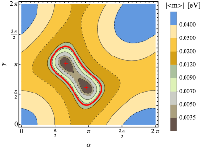
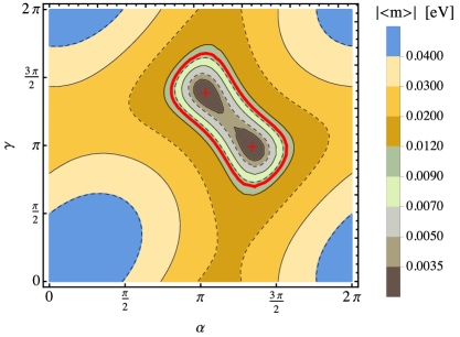
Figure 21: Left Panel. The value of $\left|\langle\!~{}m~{}\!\rangle\right|\$in the 3+2 IO scheme for $m_{3}\equiv m_{min}=0$ and the best fit values of Table 3. The phase $\eta$ is set to the value $\eta_{+}$, $\tan\eta_{+}/2\simeq-2.61$. The values of $\left|\langle\!~{}m~{}\!\rangle\right|\$ in the marked points $(\alpha,\gamma)=(3.03,1.93),(2.07,3.17)$, are zero. The red contour line corresponds to $\mbox{$\left|\langle\!~{}m~{}\!\rangle\right|\ $}=0.01$ eV. Right Panel. The same as in the left panel, but setting $\eta$ to the value $\eta_{-}$, $\tan\eta_{-}/2\simeq 2.61$. The values of $\left|\langle\!~{}m~{}\!\rangle\right|\$ in the marked points $(\alpha,\gamma)=(3.25,4.35),(4.21,3.11)$, are zero. The red contour line corresponds to $\mbox{$\left|\langle\!~{}m~{}\!\rangle\right|\ $}=0.01$ eV. See text for details.

Finally, it follows from our analysis that for $m_{3}=0$ in the cases we have considered and which are illustrated in Fig. 21 we have $\mbox{$\left|\langle\!~{}m~{}\!\rangle\right|\ $}>0.01$ eV for values of the phases $\alpha$ and $\gamma$ outside the region delimited by the red line in Fig. 21.

7 Conclusions

In the present article we have investigated the predictions for neutrinoless double beta ($(\beta\beta)_{0\nu}$-) decay effective Majorana mass $\left|\langle\!~{}m~{}\!\rangle\right|\$ in the $3+1$ and $3+2$ schemes with one and two additional sterile neutrinos with masses at the eV scale. These two schemes are widely used in the interpretation of the reactor neutrino and Gallium anomalies as well as of the data of the LSND and MiniBooNE experiments in terms of active-sterile neutrino oscillations. Due to the assumed active-sterile neutrino mixing, the “$3+1$” and “$3+2$” models have altogether 4 and 5 light massive neutrinos $\nu_{j}$ coupled to the electron and muon in the weak charged lepton current. In the minimal versions of these models the massive neutrinos are Majorana particles. The additional neutrinos $\nu_{4}$ and $\nu_{4}$, $\nu_{5}$, should have masses $m_{4}$ and $m_{4}$, $m_{5}$ at the eV scale. It follows from the data that if $\nu_{4}$ or $\nu_{4}$, $\nu_{5}$ exist, they should couple to the electron and muon in the weak charged lepton current with couplings $U_{ek}\sim 0.1$ and $U_{\mu k}\sim 0.1$, $k=4;~{}4,5$.

As was shown in [19, 20] and more recently in [21, 22, 23], the contribution of the additional light Majorana neutrinos $\nu_{4}$ or $\nu_{4,5}$ to the $(\beta\beta)_{0\nu}$-decay amplitude, and thus to the $(\beta\beta)_{0\nu}$-decay effective Majorana mass $\left|\langle\!~{}m~{}\!\rangle\right|\$, can change drastically the predictions for $\left|\langle\!~{}m~{}\!\rangle\right|\$ obtained in the reference 3-flavour neutrino mixing scheme, $|\mbox{$\langle\!~{}m~{}\!\rangle$}^{(3\nu)}|$. Using the values of the neutrino oscillation parameters of the $3+1$ and $3+2$ schemes, obtained in the global analyses of the data relevant for the active-sterile neutrino oscillation hypothesis (positive evidence and negative results), performed in [17, 18] (see Tables 1, 2 and 3), we have investigated in detail in the present article the possibility of a complete or partial cancellation among the different terms in $\left|\langle\!~{}m~{}\!\rangle\right|\$, leading to a strong suppression of $\left|\langle\!~{}m~{}\!\rangle\right|\$. This was done in the $3+1$ and $3+2$ schemes both in the cases of 3-neutrino mass spectra with normal ordering (NO) and inverted ordering (IO), as well as in the cases of normal hierarchical (NH) and inverted hierarchical (IH) spectra with ${\rm min}(m_{j})=0$, where $j=1,2,3,4$ $(j=1,2,3,4,5)$ for the $3+1$ ($3+2$) scheme. In this type of analysis the free parameters are the CP violation (CPV) Majorana phases and the lightest neutrino mass. In the case of the $3+1$ scheme, in which there are three physical CPV Majorana phases, we have found all the solutions of the system of equations which determine the minima of $\left|\langle\!~{}m~{}\!\rangle\right|\$ as well as their domains (i.e., the regions of their validity), in analytic form. This was done for all types of neutrino mass spectra we have considered. In the more complicated case of $3+2$ scheme with four physical CPV Majorana phases, the non-linearity of the system of four equations which determine the extrema of $\left|\langle\!~{}m~{}\!\rangle\right|\$makes the analytical study of the extrema of interest a complicated problem. Thus, in this case we have performed the general analysis of the minimization of $\left|\langle\!~{}m~{}\!\rangle\right|\$numerically. It was possible, however, to perform analytically the analysis of the minima of $\left|\langle\!~{}m~{}\!\rangle\right|\$, corresponding to the 16 sets of CP conserving values (either $0$ or $\pi$) of the four phases.

We have found that if the neutrino mass spectrum is of the NO type, we can have $\mbox{$\left|\langle\!~{}m~{}\!\rangle\right|\ $}=0$, and thus strongly suppressed $\left|\langle\!~{}m~{}\!\rangle\right|\$, in a specific interval of values of ${\rm min}(m_{j})\equiv m_{min}$, $\underline{m}_{1}\leq m_{min}\leq\overline{m}_{1}$. This results is valid both for the $3+1$ and $3+2$ schemes. The specific values of $\underline{m}_{1}$ and $\overline{m}_{1}$ depend on the scheme: they are determined by the values of the oscillation parameters in each of the two schemes. For the best fit values reported in Tables 1, 2 and 3, in the $3+1$ with $\Delta m^{2}_{41}=0.93\,{\rm eV^{2}}$, $3+1$ with $\Delta m^{2}_{41}=1.78\,{\rm eV^{2}}$ and $3+2$ schemes they read, respectively: $(\underline{m}_{1},\overline{m}_{1})=(0.021,0.065)$ eV, $(\underline{m}_{1},\overline{m}_{1})=(0.030,0.091)$ eV and $(0.004,0.088)$ eV. For the different values of $m_{min}$ from the indicated interval, the minimum $\mbox{$\left|\langle\!~{}m~{}\!\rangle\right|\ $}=0$ is reached for different sets of CP nonconserving, in general, values of the CPV Majorana phases.

For the best fit values reported in Tables 1, 2 and 3, we find that we always have $\mbox{$\left|\langle\!~{}m~{}\!\rangle\right|\ $}>0.01$ eV,

• in the $3+1$ scheme with $\Delta m^{2}_{41}=0.93~{}{\rm eV^{2}}$ – for $m_{min}<0.010$ eV and $m_{min}>0.093$ eV;

• in the $3+1$ scheme with $\Delta m^{2}_{41}=1.78~{}{\rm eV^{2}}$ – for $m_{min}<0.020$ eV and $m_{min}>0.119$ eV;

• in the $3+2$ scheme – for $m_{min}>0.118$ eV.

The results we have obtained for IO spectrum are different. In this case one can have $\mbox{$\left|\langle\!~{}m~{}\!\rangle\right|\ $}=0$ in the interval $m_{min}\leq\overline{m}_{3}$, where $\overline{m}_{3}$ is determined by the values of neutrino oscillation parameters. For a given $m_{min}$ from the indicated interval, $\mbox{$\left|\langle\!~{}m~{}\!\rangle\right|\ $}=0$ takes place for specific, in general, CP nonconserving values of the relevant Majorana phases. The values of $\overline{m}_{3}$ in the two schemes, $3+1$ and $3+2$, differ. Using the values of the oscillation parameters given in Tables 1, 2 and 3, we find: $\overline{m}_{3}=0.038\,(0.074)$ eV for $\Delta m^{2}_{41}=0.93\,(1.78)\,{\rm eV^{2}}$ in the $3+1$ scheme, and $\overline{m}_{3}=0.125$ in the $3+2$ scheme.

Using the values of the oscillation parameters given in Tables 1, 2 and 3, we find also that one has always $\mbox{$\left|\langle\!~{}m~{}\!\rangle\right|\ $}>0.01$ eV,

• in the $3+1$ scheme with $\Delta m^{2}_{43}=0.93~{}{\rm eV^{2}}$ – for $m_{min}>0.078$ eV;

• in the $3+1$ scheme with $\Delta m^{2}_{43}=1.78~{}{\rm eV^{2}}$ – for $m_{min}>0.108$ eV;

• in the $3+2$ scheme – for $m_{min}>0.178$ eV.

We have investigated also the specific cases of NH and IH spectra in the limit $m_{min}=0$, which present certain peculiarities both in the $3+1$ and $3+2$ schemes.

The analysis performed by us allowed to derive the general conditions under which the effective Majorana mass satisfies $\mbox{$\left|\langle\!~{}m~{}\!\rangle\right|\ $}>0.01$ eV, and thus to determine the regions of values $m_{min}$ for which $\left|\langle\!~{}m~{}\!\rangle\right|\$is predicted to lie in the range planned to be explored by the next generation of $(\beta\beta)_{0\nu}$-experiments. The results of these experiments will provide additional tests of the hypothesis of existence of sterile neutrinos with masses at the eV scale, and couplings $\sim 0.1$ to the electron and muon in the weak charged lepton current.

Appendix A The Extrema of $\left|\langle\!~{}m~{}\!\rangle\right|\$in the 3+1 Scheme with NO or IO Neutrino Mass Spectrum

We are interested in the minima and the maxima of $\left|\langle\!~{}m~{}\!\rangle\right|\$. It turns out to be somewhat simpler to study the extrema of $\mbox{$\left|\langle\!~{}m~{}\!\rangle\right|\ $}^{2}$ which obviously coincide with those of $\left|\langle\!~{}m~{}\!\rangle\right|\$. The expression for $\mbox{$\left|\langle\!~{}m~{}\!\rangle\right|\ $}^{2}$ in both the cases of NO and IO spectra can be written as:

$$\mbox{$\left|\langle\!~{}m~{}\!\rangle\right|\ $}^{2}=|a+e^{i\alpha}b+e^{i\beta}c+e^{i\gamma}d|^{2}.$$ (47)

The zeros of the first derivatives of $\mbox{$\left|\langle\!~{}m~{}\!\rangle\right|\ $}^{2}$ with respect to the phases $\alpha$, $\beta$ and $\gamma$ are given by the following system of three equations:

$$\begin{split}-&2b[a\sin(\alpha)+c\sin(\alpha-\beta)+d\sin(\alpha-\gamma)]=0,\\ -&2c[a\sin(\beta)-b\sin(\alpha-\beta)+d\sin(\beta-\gamma)]=0,\\ &2d[-a\sin(\gamma)+b\sin(\alpha-\gamma)+c\sin(\beta-\gamma)]=0.\\ \end{split}$$ (48)

In order to solve this system we use the following parametrization:

$$\begin{split}&\sin\alpha=\frac{2v}{1+v^{2}},\qquad\cos\alpha=\frac{1-v^{2}}{1+v^{2}},\\ &\sin\beta=\frac{2t}{1+t^{2}},\qquad\cos\beta=\frac{1-t^{2}}{1+t^{2}},\\ &\sin\gamma=\frac{2u}{1+u^{2}},\qquad\cos\gamma=\frac{1-u^{2}}{1+u^{2}}.\\ \end{split}$$ (49)

where, respectively, $v\equiv\tan(\alpha/2)$, $t\equiv\tan(\beta/2)$, $u\equiv\tan(\gamma/2)$ with $\alpha$, $\beta$, $\gamma\neq\pi+2k\pi$. In terms of the new variables the system in eq.(48) can be written as:

$$\begin{split}-&\frac{2b}{1+v^{2}}\bigg{[}2av-\frac{2ct\left(1-v^{2}\right)}{t^{2}+1}+\frac{2c\left(1-t^{2}\right)v}{t^{2}+1}-\frac{2du\left(1-v^{2}\right)}{u^{2}+1}+\frac{2d\left(1-u^{2}\right)v}{u^{2}+1}\bigg{]}=0,\\ -&\frac{2c}{1+t^{2}}\bigg{[}2at-\frac{2b\left(1-t^{2}\right)v}{v^{2}+1}+\frac{2bt\left(1-v^{2}\right)}{v^{2}+1}-\frac{2d\left(1-t^{2}\right)u}{u^{2}+1}+\frac{2dt\left(1-u^{2}\right)}{u^{2}+1}\bigg{]}=0,\\ &\frac{2d}{1+u^{2}}\bigg{[}-2au+\frac{2b\left(1-u^{2}\right)v}{v^{2}+1}-\frac{2bu\left(1-v^{2}\right)}{v^{2}+1}+\frac{2ct\left(1-u^{2}\right)}{t^{2}+1}-\frac{2c\left(1-t^{2}\right)u}{t^{2}+1}\bigg{]}=0.\\ \end{split}$$ (50)

The new coordinates $u$, $v$ and $t$ are singular if at least one angle $\alpha,\beta,\gamma$ is equal to $\pi$. We observe that seven solutions of the system in eq. (48) are given for one of the three phases equal to $\pi$, i.e., for $u$ or $v$ or $t$ going to $\infty$:

$$\begin{split}\alpha&=\beta=\pi(0)\quad\mbox{and}\quad\gamma=0(\pi),\\ \alpha&=\gamma=\pi(0)\quad\mbox{and}\quad\beta=0(\pi),\\ \gamma&=\beta=\pi(0)\quad\mbox{and}\quad\alpha=0(\pi),\\ \alpha&=\beta=\gamma=\pi\,\,.\\ \end{split}$$ (51)

We can recover this type of solutions as a limit of the system in eq. (50) when a pair of variables $u$, $v$, $t$ are equal. For example, in the limit in which $t=v=0$, the system in eq. (50) is reduced to

$$\begin{split}\begin{cases}&(4bd)\dfrac{u}{u^{2}+1}=0,\\ &(4cd)\dfrac{u}{u^{2}+1}=0,\\ &[4d(a+b+c)]\dfrac{u}{u^{2}+1}=0\,.\\ \end{cases}\end{split}$$ (52)

Evidently, we have a solution in the limit $u\rightarrow\infty$. This is equivalent to say that the solutions under discussion can be found as a limit of the system (50) when the variables $u$, $t$, and $v$ are sent to $\infty$.

The solutions of the system in eq. (50), assuming $\alpha,\beta,\gamma\neq\pi$ and $b,c,d\neq 0$, are the zeros of the following system of equations:

$$\begin{split}\begin{cases}&2av-\dfrac{2ct\left(1-v^{2}\right)}{t^{2}+1}+\dfrac{2c\left(1-t^{2}\right)v}{t^{2}+1}-\dfrac{2du\left(1-v^{2}\right)}{u^{2}+1}+\dfrac{2d\left(1-u^{2}\right)v}{u^{2}+1}=0,\\ &2at-\dfrac{2b\left(1-t^{2}\right)v}{v^{2}+1}+\dfrac{2bt\left(1-v^{2}\right)}{v^{2}+1}-\dfrac{2d\left(1-t^{2}\right)u}{u^{2}+1}+\dfrac{2dt\left(1-u^{2}\right)}{u^{2}+1}=0,\\ &-2au+\dfrac{2b\left(1-u^{2}\right)v}{v^{2}+1}-\dfrac{2bu\left(1-v^{2}\right)}{v^{2}+1}+\dfrac{2ct\left(1-u^{2}\right)}{t^{2}+1}-\dfrac{2c\left(1-t^{2}\right)u}{t^{2}+1}=0.\\ \end{cases}\end{split}$$ (53)

The solutions of this system are nine: $(u_{1},v_{1},t_{1})$, $(u_{\pm},v_{\pm},t_{\pm})$, $(u^{\pm}_{i},v^{\pm}_{i},t^{\pm}_{i})$ with $i=2,3$ and $(v^{\pm}_{4}(u),t^{\pm}_{4}(u))$. We found $(u_{1},v_{1},t_{1})=(0,0,0)$ and

$$\begin{split}&\begin{cases}u_{\pm}&=\pm\sqrt{\dfrac{(-a+b+c-d)(a+b-c+d)}{(a-b-c-d)(a+b-c-d)}},\\ v_{\pm}&=\pm\dfrac{(b+c)}{(b-c)}\dfrac{[(a+b-c)^{2}-d^{2}]}{\sqrt{(-a+b+c-d)(a+b-c+d)(a-d-c-b)(a-d-c+b)}},\\ t_{\pm}&=\pm\dfrac{a^{2}+b^{2}-c^{2}-d^{2}}{\sqrt{(a-b-c-d)(a+b-c-d)(-a+b+c-d)(a+b-c+d)}},\\ \end{cases}\\ &\\ &\begin{cases}u^{\pm}_{2}&=0,\\ v^{\pm}_{2}&=\pm\sqrt{\dfrac{(-a-b+c-d)(a+b+c+d)}{(a-b-c+d)(a-b+c+d)}},\\ t^{\pm}_{2}&=\pm\dfrac{(a-b+c+d)(a+b+c+d)}{\sqrt{(a-b-c+d)(a-b+c+d)(-a-b+c-d)(a+b+c+d)}},\\ \end{cases}\\ &\\ &\begin{cases}u^{\pm}_{3}&=\pm\sqrt{\dfrac{(-a+b+c-d)(a-b+c+d)}{(a-b-c-d)(a-b+c-d)}},\\ v^{\pm}_{3}&=\pm\dfrac{a^{2}-b^{2}+c^{2}-d^{2}}{\sqrt{(a-b-c-d)(a-b+c-d)(-a+b+c-d)(a-b+c+d)}},\\ t^{\pm}_{3}&=\pm\dfrac{(b+c)(-a+b-c+d)}{(b-c)(-a+b+c-d)}\sqrt{\dfrac{(-a+b+c-d)(a-b+c+d)}{(a-b-c-d)(a-b+c-d)}},\\ \end{cases}\\ &\\ &\begin{cases}v^{\pm}_{4}(u)&=\dfrac{4bdu\pm F(a,b,c,d,u)}{-u^{2}(a-b-c-d)(a-b+c-d)-(a-b+d)^{2}+c^{2}},\\ t^{\pm}_{4}(u)&=\dfrac{-4cdu\pm F(a,b,c,d,u)}{u^{2}(a-b-c-d)(a+b-c-d)+(a-c+d)^{2}-b^{2}},\\ \end{cases}\\ \end{split}$$ (54)

where

$$\begin{split}F(a,b,c,d,u)&=\bigg{\{}\Big{[}-u^{2}(a+b-c-d)(a-b+c-d)-(a+d)^{2}+(b-c)^{2}\Big{]}\times\\ &\times\Big{[}a^{2}\left(u^{2}+1\right)-2ad\left(u^{2}-1\right)-\left(u^{2}+1\right)(b+c-d)(b+c+d)\Big{]}\bigg{\}}^{1/2}.\\ \end{split}$$

We observe that in the NH case, the limit $m_{1}\rightarrow 0$ corresponds to setting $a\rightarrow 0$ in eqs. (50), while the limit $m_{3}\rightarrow 0$ in the IH case corresponds to $c\rightarrow 0$. We define the constants $a,b,c,d$ in these limits respectively as $b_{0},c_{0},d_{0}$ and $a_{0},b_{0},d_{0}$. Moreover, we observe that $\left|\langle\!~{}m~{}\!\rangle\right|\$evaluated at the solutions $(u^{\pm}_{i},v^{\pm}_{i},t^{\pm}_{i})$ with $i=2,3$, $(v^{\pm}_{4},t^{\pm}_{4})$ and $(u_{\pm},v_{\pm},t_{\pm})$ is exactly zero.

In the subsection 6.2 we discuss, in particular, the limiting case of $m_{3}\rightarrow 0$. Therefore it is useful to show the solutions $(u_{\pm},v_{\pm},t_{\pm})$ in terms of $\sin\gamma_{+}=-\sin\gamma_{-}$, $\sin\alpha_{+}=-\sin\alpha_{-}$, $\sin\beta_{+}=-\sin\beta_{-}$, so we can write:

$$\begin{split}\sin\gamma_{-}&=\frac{\sqrt{-[(a-d-c)^{2}-b^{2}][(a+d-c)^{2}-b^{2}]}}{2(a-c)d}\,,\\ \sin\alpha_{-}&=\frac{(b-c)(b+c)(a+b-c-d)\sqrt{(-a+b+c-d)(a+b-c+d)}(-a+b+c+d)}{2\left(ab\left(c(a-c)+b^{2}\right)-bcd^{2}\right)\sqrt{(-a+c+d)^{2}-b^{2}}}\,,\\ \sin\beta_{-}&=\frac{\sqrt{(a-b-c-d)(a+b-c-d)}\sqrt{(-a+b+c-d)(a+b-c+d)}\left(-a^{2}-b^{2}+c^{2}+d^{2}\right)}{2(a-c)\left[a\left(c(a-c)+b^{2}\right)-cd^{2}\right]}\,.\\ \end{split}$$

Next, in order to study the domains of existence of the solutions given in eq. (54), which depend on the parameters $a$ $b$, $c$ and $d$, we need to define the following functions:

$$\begin{split}f_{1}&=a-b-c-d\,,\qquad f_{2}=a+b-c-d\,,\\ f_{3}&=a+b-c+d\,,\qquad f_{4}=-a+b+c-d\,,\\ f_{5}&=a+b+c+d\,,\qquad f_{6}=a-b+c+d\,,\\ f_{7}&=a-b+c-d\,,\qquad f_{8}=a+b+c-d\,.\\ \end{split}$$ (55)

We notice that the conditions of existence for the solutions $(u_{\pm},v_{\pm},t_{\pm})$, $(u^{\pm}_{2},v^{\pm}_{2},t^{\pm}_{2})$ and $(u^{\pm}_{3},v^{\pm}_{3},t^{\pm}_{3})$ are respectively $f_{3}f_{4}f_{5}f_{6}>0$, $f_{1}f_{4}f_{6}f_{7}>0$ and $f_{1}f_{2}f_{3}f_{4}>0$. We discuss the domains of the other solutions in Appendix A.1 using numerical methods.

Finally, we would like to comment on the solutions $(v^{\pm}_{4},t^{\pm}_{4})$ because, as can be seen from their explicit expressions, they depend on a free variable, $u$. Thus, we would like to provide some details about the study of the domain of such solutions. Defining $k=u^{2}$ and $F(a,b,c,d,k)=\sqrt{f(k)}$ we find that the function $f(k)$ is a parabola of the form:

$$f(k)=Ak^{2}+Bk+C\,,$$ (56)

with coefficient of the term of maximum degree equal to

$$A=(a+b-c-d)(a-b+c-d)(a+b+c-d)(-a+b+c+d)\,,$$ (57)

and discriminant $\Delta=B^{2}-4AC=256\,a^{2}b^{2}c^{2}d^{2}$. The discriminant $\Delta$ is always positive or equal to zero. The zeros of the function $f(k)$, namely $k_{1}$ and $k_{2}$, are given by:

$$\begin{split}\tilde{k}_{1}&=\frac{(a-b-c+d)(a+b+c+d)}{(a+b+c-d)(-a+b+c+d)}\,,\\ \tilde{k}_{2}&=-\frac{(a+b-c+d)(a-b+c+d)}{(a+b-c-d)(a-b+c-d)}\,.\\ \end{split}$$ (58)

Depending on the values of the parameters $a,b,c$ and $d$ one can find a range of $m_{min}$ for which this solution is well defined. We will discuss this in the next section A.1.

The method described above cannot be used to determine the physical domain of the minimization solutions found by us in the case in which at least one of the phases $\alpha,\beta,\gamma$ is equal to $\pi$ (eq. (LABEL:solpi)). In order to study these cases we use the Hessian matrix of $\mbox{$\left|\langle\!~{}m~{}\!\rangle\right|\ $}^{2}$, $H(\alpha,\beta,\gamma)$. The determinant of the Hessian, evaluated for the phases either $0$ or $\pi$ and assuming $a,b,c,d>0$, can be positive only for $(\alpha,\beta,\gamma)=(\pi,0,0),(0,\pi,0),(0,0,\pi),(\pi,\pi,\pi)$. Therefore the local minima and maxima can correspond only to these configurations. We derive the relations among the coefficients $a,b,c,d$ in order to have a minimum using the Sylvester’s criterion. We assume that $a,b,c,d$ are real and positive, $a,b,c,d>0$.
We have a minima at

$$\begin{split}(\alpha,\beta,\gamma)&=(\pi,\pi,\pi)\quad if\quad f_{1}=a-b-c-d>0;\\ (\alpha,\beta,\gamma)&=(0,0,\pi)\quad if\quad(c<d)\land(b<d-c)\land(f_{8}=a+b+c-d<0);\\ (\alpha,\beta,\gamma)&=(0,\pi,0)\quad if\quad(c>d)\land(b<c-d)\land(-f_{3}=-a-b+c-d>0);\\ (\alpha,\beta,\gamma)&=(\pi,0,0)\quad if\quad(b>c+d)\land(-f_{6}=-a+b-c-d>0).\\ \end{split}$$ (59)

A.1 Domains of the solutions

In this part we describe the domains of the solutions given in eq. (54). We will give the numerical intervals of values of $m_{min}$ in which the minimization solutions are well defined for $\Delta m^{2}_{41(43)}=0.93~{}{\rm eV^{2}}$ and $1.78~{}{\rm eV^{2}}$ and using the best fit values reported in Table 1. In Tables 4 and 5 we present the results of this numerical analysis in the cases of NO and IO spectra, respectively.

Solution	Domain of existence in terms of $m_{min}$
$(u^{\pm},v^{\pm},t^{\pm})$	$2.363\times 10^{-2}\,{\rm eV}<m_{1}<6.473\times 10^{-2}\,{\rm eV}$
	($3.337\times 10^{-2}\,{\rm eV}<m_{1}<9.061\times 10^{-2}\,{\rm eV}$)
$(u^{\pm}_{2},v^{\pm}_{2},t^{\pm}_{2})$	None
	(None)
$(u^{\pm}_{3},v^{\pm}_{3},t^{\pm}_{3})$	$5.485\times 10^{-2}\,{\rm eV}<m_{1}<6.473\times 10^{-2}\,{\rm eV}$
	($7.811\times 10^{-2}\,{\rm eV}<m_{1}<9.061\times 10^{-2}\,{\rm eV}$)
$(v^{\pm}_{4},t^{\pm}_{4})$ for $A>0$	$2.090\times 10^{-2}\,{\rm eV}<m_{1}<2.363\times 10^{-2}\,{\rm eV}\,\,\,\lor$
	$\lor\,\,\,5.485\times 10^{-2}\,{\rm eV}<m_{1}<6.473\times 10^{-2}\,{\rm eV}$
	($3.043\times 10^{-2}\,{\rm eV}<m_{1}<3.337\times 10^{-2}\,{\rm eV}\,\,\,\lor$
	$\lor\,\,\,7.811\times 10^{-2}\,{\rm eV}<m_{1}<9.061\times 10^{-2}\,{\rm eV}$)
$(v^{\pm}_{4},t^{\pm}_{4})$ for $A<0$	$2.363\times 10^{-2}\,{\rm eV}<m_{1}<5.485\times 10^{-2}\,{\rm eV}$
	($3.337\times 10^{-2}\,{\rm eV}<m_{1}<7.811\times 10^{-2}\,{\rm eV}$)

Table 4: Numerical results for the domains of existence of the solutions given in eq. (54) in the 3+1 NO case for $\Delta m^{2}_{41}=0.93\,{\rm eV^{2}}$ ($\Delta m^{2}_{41}=1.78\,{\rm eV^{2}}$). The expression of $A$ is given in eq. (57).

Solution	Domain of existence in terms of $m_{min}$
$(u^{\pm},v^{\pm},t^{\pm})$	$0\,{\rm eV}<m_{3}<3.855\cdot 10^{-2}\,{\rm eV}$
	($0\,{\rm eV}<m_{3}<7.437\times 10^{-2}\,{\rm eV}$)
$(u^{\pm}_{2},v^{\pm}_{2},t^{\pm}_{2})$	None
	(None)
$(u^{\pm}_{3},v^{\pm}_{3},t^{\pm}_{3})$	$3.084\times 10^{-2}\,{\rm eV}<m_{3}<3.855\times 10^{-2}\,{\rm eV}$
	($6.344\times 10^{-2}\,{\rm eV}<m_{3}<7.437\times 10^{-2}\,{\rm eV}$)
$(v^{\pm}_{4},t^{\pm}_{4})$ for $A>0$	$3.084\times 10^{-2}\,{\rm eV}<m_{3}<3.855\times 10^{-2}\,{\rm eV}$
	($6.344\times 10^{-2}\,{\rm eV}<m_{3}<7.437\times 10^{-2}\,{\rm eV}$)
$(v^{\pm}_{4},t^{\pm}_{4})$ for $A<0$	$0\,{\rm eV}<m_{3}<3.084\times 10^{-2}\,{\rm eV}$
	($0\,{\rm eV}<m_{3}<6.344\times 10^{-2}\,{\rm eV}$)

Table 5: The same as in Table 4 but for the case of the 3+1 IO scheme.

Appendix B Extrema of $\left|\langle\!~{}m~{}\!\rangle\right|\$in the 3+2 Scheme

As in the case of the 3+1 scheme, it proves somewhat easier to study the extrema of $\mbox{$\left|\langle\!~{}m~{}\!\rangle\right|\ $}^{2}$ than of $\left|\langle\!~{}m~{}\!\rangle\right|\$. The expression for $\mbox{$\left|\langle\!~{}m~{}\!\rangle\right|\ $}^{2}$ for both NO and IO spectra has the form:

$$\mbox{$\left|\langle\!~{}m~{}\!\rangle\right|\ $}^{2}=|a+e^{i\alpha}b+e^{i\beta}c+e^{i\gamma}d+e^{i\eta}e|^{2}.$$ (60)

Equating to zero the first derivatives of $\mbox{$\left|\langle\!~{}m~{}\!\rangle\right|\ $}^{2}$ with respect to the four phases we get the following system of four equations:

$$\begin{split}&a\sin(\alpha)+c\sin(\alpha-\beta)+d\sin(\alpha-\gamma)+e\sin(\alpha-\eta)=0,\\ &a\sin(\beta)-b\sin(\alpha-\beta)+d\sin(\beta-\gamma)+e\sin(\beta-\eta)=0,\\ -&a\sin(\gamma)+b\sin(\alpha-\gamma)+c\sin(\beta-\gamma)-e\sin(\gamma-\eta)=0,\\ -&a\sin(\eta)+b\sin(\alpha-\eta)+c\sin(\beta-\eta)+d\sin(\gamma-\eta)=0.\\ \end{split}$$ (61)

The analytical study of the minima of $\mbox{$\left|\langle\!~{}m~{}\!\rangle\right|\ $}^{2}$ in this case is a non-trivial task since four phases are involved and the non-linearity of the system of the first derivatives of $\mbox{$\left|\langle\!~{}m~{}\!\rangle\right|\ $}^{2}$ with respect to the four phases makes the analysis rather complicated. Therefore finding all possible solutions of the minimization procedure in analytical form is a complicated problem. Thus, we have performed the general analysis of the minimization of $\left|\langle\!~{}m~{}\!\rangle\right|\$numerically. This allowed to determine the intervals of values of $m_{min}$ in which the minimal value of $\left|\langle\!~{}m~{}\!\rangle\right|\$is exactly zero. It is possible, however, to perform analytically the analysis of the minima of $\left|\langle\!~{}m~{}\!\rangle\right|\$, corresponding to the 16 sets of CP conserving values (either $0$ or $\pi$) of the four phases $\alpha$, $\beta$, $\gamma$ and $\eta$. This can be done by using the Sylvester’s criterion for the Hessian, evaluated for the indicated values of the phases $0,\pi$, which determines the physical domain of the minimization solutions. The minima thus found, as we show, correspond to $\mbox{$\left|\langle\!~{}m~{}\!\rangle\right|\ $}\neq 0$.

Assuming $a,b,c,d,e>0$ and $a,b,c,d,e\in\mathbb{R}$ and using the Sylvester’s criterion we find that the minima of $\left|\langle\!~{}m~{}\!\rangle\right|\$take place at

$$\begin{split}(\alpha,\beta,\gamma,\eta)&=(\pi,\pi,\pi,\pi)\quad if\quad F_{1}=a-b-c-d-e>0,\\ (\alpha,\beta,\gamma,\eta)&=(0,0,0,\pi)\quad if\quad(d<e)\land(c<e-d)\land(b<-c-d+e)\land\\ &\phantom{,aaaaaaaaaaaaaaa}\land(F_{8}=a+b+c+d-e<0),\\ (\alpha,\beta,\gamma,\eta)&=(0,0,\pi,0)\quad if\quad(d>e)\land(c<d-e)\land(b<-c+d-e)\land\\ &\phantom{,aaaaaaaaaaaaaaa}\land(F_{3}=a+b+c-d+e<0),\\ (\alpha,\beta,\gamma,\eta)&=(0,\pi,0,0)\quad if\quad(c>d+e)\land(b<c-d-e)\land\\ &\phantom{,aaaaaaaaaaaaaaa}\land(G_{3}=a+b-c+d+e<0),\\ (\alpha,\beta,\gamma,\eta)&=(\pi,0,0,0)\quad if\quad(b>c+d+e)\land(F_{6}=a-b+c+d+e<0)\,.\end{split}$$ (62)

At the other CP conserving values of the phases, $(\alpha,\beta,\gamma,\eta)$ = $(0,0,0,0)$, $(\pi,\pi,0,0)$, $(\pi,0,\pi,0)$, $(\pi,0,0,\pi)$, $(0,\pi,\pi,0)$, $(0,\pi,0,\pi)$, $(0,0,\pi,\pi)$, $(\pi,\pi,\pi,0)$, $(\pi,\pi,0,\pi)$, $(\pi,0,\pi,\pi)$ and $(0,\pi,\pi,\pi)$, $\left|\langle\!~{}m~{}\!\rangle\right|\$cannot reach a minimum. In Fig. 22 we show the dependence of the functions $F_{1}$, $F_{8}$, $F_{3}$, $G_{3}$ and $F_{6}$ on $m_{min}\equiv m_{3}$ for the best fit values of the neutrinos oscillation parameters given in Tables 1 and 3.

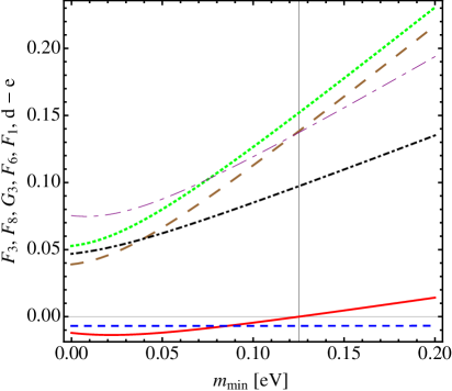
Figure 22: The functions $F_{3}$ (dotted green line), $F_{8}$ (long-dashed brown line), $G_{3}$ (short-long-dashed purple line), $F_{6}$ (dot-dashed black line), $F_{1}$ (solid red line), $d-e$ (short-dashed blue line), defined in eq. (35), versus $m_{min}\equiv m_{3}$ for the oscillation parameter values reported in Table 3. The vertical black line corresponds to $m_{min}=\overline{m}_{3}\simeq 1.25\times 10^{-1}\,{\rm eV}$.

References

- [1] K. Nakamura and S. T. Petcov, in J. Beringer et al. (Particle Data Group), Phys. Rev. D 86 (2012) 010001.
- [2] G. L. Fogli, E. Lisi, A. Marrone, D. Montanino, A. Palazzo and A. M. Rotunno, Phys. Rev. D 86 (2012) 013012.
- [3] M. C. Gonzalez-Garcia, M. Maltoni, J. Salvado and T. Schwetz, JHEP 1212 (2012) 123.
- [4] K.N. Abazajian et al., “Light Sterile Neutrinos: A White Paper”, arXiv:1204.5379
- [5] B. Armbruster et al. [KARMEN Collab.], Phys. Rev. D 65 (2002) 112001.
- [6] P. Astier et al. [NOMAD Collab.], Phys. Lett. B570 (2003) 19.
- [7] M. Antonello et al. [ICARUS Collab.], Eur. Phys. J. C73 (2013) 2345.
- [8] F. Dydak et al. [CDHSW Collab.], Phys. Lett. B134 (1984) 281.
- [9] P. Adamson et al. [MINOS Collab.], Phys. Rev. Lett. 107 (2011) 011802.
- [10] R. Wendell et al. [Super-Kamiokande Collab.], Phys. Rev. D 81 (2010) 092004.
- [11] P. A. R. Ade et al. [Planck Collaboration], arXiv:1303.5076 [astro-ph.CO].
- [12] S. Gariazzo, C. Giunti and M. Laveder, arXiv:1309.3192.
- [13] N. Saviano et al., Phys. Rev. D 87 (2013) 073006; S. Hannestad, R.S. Hansen and T. Tram, JCAP 1304 (2013) 032.
- [14] A. Mirizzi et al., arXiv:1303.5368 [astro-ph.CO].
- [15] M. Wyman, D. H. Rudd, R. A. Vanderveld and W. Hu, arXiv:1307.7715 [astro-ph.CO].
- [16] R. Laureijs, J. Amiaux, S. Arduini, J. -L. Augueres, J. Brinchmann, R. Cole, M. Cropper and C. Dabin et al., arXiv:1110.3193 [astro-ph.CO].
- [17] C. Giunti, M. Laveder, Y. F. Li and H. W. Long, arXiv:1308.5288 [hep-ph].
- [18] J. Kopp, P. A. N. Machado, M. Maltoni and T. Schwetz, JHEP 1305 (2013) 050.
- [19] S.M. Bilenky, S. Pascoli and S.T. Petcov, Phys. Rev. D 64 (2001) 113003.
- [20] S. Goswami and W. Rodejohann, Phys. Rev. D 73 (2006) 113003.
- [21] Barry, W. Rodejohann and Zhang, JHEP 07 (2011) 091; W. Rodejohann, J. Phys. G 39 (2012) 124008.
- [22] Y.F. Li and Si-shuo Liu, Phys. Lett. B 706 (2012) 406.
- [23] M. Ghosh, S. Goswami, S. Gupta and C.S. Kim, arXiv:1305.0180.
- [24] S.M. Bilenky and S.T. Petcov, Rev. Mod. Phys. 59 (1097) 671.
- [25] W. Rodejohann, Int. J. Mod. Phys. E 20 (2011) 1833; see also, e.g., S.T. Petcov, Physica Scripta T 121 (2005) 94 [hep-ph/0504166].
- [26] S.M. Bilenky, S. Pascoli and S.T. Petcov, Phys. Rev. D 64 (2001) 053010.
- [27] S. Pascoli and S.T. Petcov, Phys. Lett. B 544 (2002) 239; Phys. Lett. B 580 (2004) 280.
- [28] S. T. Petcov, Adv. High Energy Phys. 2013 (2013) 852987 [arXiv:1303.5819].
- [29] S.M. Bilenky, J. Hosek and S.T. Petcov, Phys. Lett. B 94 (1980) 495.
- [30] M. Archidiacono, N. Fornengo, C. Giunti and A. Melchiorri, Phys. Rev. D 86 (2012) 065028.
- [31] A. A. Aguilar-Arevalo et al. [MiniBooNE Collaboration], Phys. Rev. Lett. 98 (2007) 231801 [arXiv:0704.1500 [hep-ex]]; Phys. Rev. Lett. 102 (2009) 101802. [arXiv:0812.2243 [hep-ex]]. Phys. Rev. Lett. 110 (2013) 161801 [arXiv:1207.4809 [hep-ex], arXiv:1303.2588 [hep-ex]].
- [32] S. Pascoli and S. T. Petcov, Phys. Rev. D 77 (2008) 113003 [arXiv:0711.4993 [hep-ph]].
- [33] M. Agostini et al., arXiv:1307.4720 [nucl-ex].
- [34] R. G. H. Robertson et al. [KATRIN Collaboration], arXiv:1307.5486 [hep-ex].