Local dynamics of a randomly pinned crack front: A numerical study

Abstract

We investigate numerically the dynamics of crack propagation along a weak plane using a model consisting of fibers connecting a soft and a hard clamp. This bottom-up model has previously been shown to contain the competition of two crack propagation mechanisms: coalescence of damage with the front on small scales and pinned elastic line motion on large scales. We investigate the dynamical scaling properties of the model, both on small and large scale. The model results compare favorable with experimental results.

I Introduction

The motion of a fracture front through a disordered medium is for obvious reasons of great practical importance. Nevertheless, it is a very complex problem which have kept materials scientists and mechanical engineers occupied for almost two centuries l93 . In an attempt to simplify the problem, Schmittbuhl et al. srvm95 proposed to study the motion of a fracture front moving along a weak plane, thereby supressing the out of plane motion of the front. In a seminal experimental study, Schmittbuhl and Måløy sm97 followed this idea up by sintering two sandblasted plexiglass plates together and then plying them apart from one edge. The sintering made the otherwise due to the sandblasting, opaque plates transparent. Where the plates were broken apart again, the opaqueness returned. Hence, it was possible to identify and follow the motion of the front since the plates would be transparent in front of the crack front and opaque behind it. There have been a large number of studies on this system following this initial work. Most of these studies have been theoretical or numerical in character and they have mostly dealt with the roughness of the crack front, see e.g. ref97 ; dsm99 ; rk02 ; shb03 ; sgtshm10 . See also the recent reviews by Bonamy and Bonamy and Bouchaud b09 ; bb11 .

The roughness is only one aspect of the motion of the crack front in this system. A first study of the dynamics of the front was published by Måløy and Schmittbuhl in 2001 ms01 . The velocity distribution was measured and found to decay slower than an exponential. This was followed by a study by Måløy et al. msst06 introducing the waiting time matrix technique making it possible to measure pixel by pixel the time the front sits still locally. This revealed an avalanche structure where portions of the front would sweep an area $S$ with a velocity $v$ before halting again. Both the distribution of areas and velocities were power laws. In two later papers, Tallakstad et al. ttssm11 and Lengliné et al. ltseatsm11 , have continued and refined this work.

The fluctuating line model, based on the idea that the crack front moves as a pinned elastic line srvm95 ; bblp93 , dominates the theoretical descriptions of the constrained crack problem. It is a top-down approach where the motion of the crack front is derived from continuum elastic theory. Its earliest use was to calculate the roughness exponent controlling the scaling properties of the crack front. If $h(x,t)$ is the position of the crack front at time $t$ and position $x$ along its base line, then one finds the height-height correlation function $\langle(h(x+\Delta x)-h(x))^{2}\rangle$ scaling as $|\Delta x|^{\zeta}$ where $\zeta$ is the rougness exponent srvm95 . The most presise measurement of the roughness exponent withing the fluctuating line model to date is $\zeta=0.388\pm 0.002$ rk02 . However, the experimental measurements of the $\zeta$ gave systematically a much larger value, namely around 0.6 — Schmittbuhl and Måloy sm97 found $\zeta=0.55\pm 0.05$ and Delaplace et al. dsm99 $\zeta=0.63\pm 0.03$.

Santucci et al. sgtshm10 has reanalyzed data from a number of earlier studies, including dsm99 , finding that the crack front has two scaling regimes: one small-scale regime described by a roughness exponent $\zeta_{-}=0.60\pm 0.05$ and a large-scale regime described by a roughness exponent $\zeta_{+}=0.35\pm 0.05$. Hence, there is a large scale roughness regime which is consistent with the fluctuating line model. However, the small scale regime is too rough. Laurson et al. lsz10 has linked this regime to correlations in the pinning strength below the Larkin lenght within the fluctuating line model. This approach assumes that the physics behind both scaling regimes is describable within the same top-down model.

A very different approach to explain the roughness of the crack front has been proposed by Schmittbuhl et al. shb03 . It is a bottom-up approach based on a stress-weighted gradient percolation process. This idea in turn has its origin in the proposal by Bouchaud et al. bbfrr02 that the crack front does not advance not only due to a competition between effective elastic forces and pinning forces at the front, but also by coalescence of damage in front of the crack with the advancing crack itself. The coalescence

By refining the model proposed by Batrouni et al. bhs02 ; gsh12 , consisting of fibers clamped between a hard and a soft block and with a gradient in the breaking thresholds, we have identified two scaling regimes for the roughness of the advancing crack front gsh13 . On large scales we recover the roughness seen in the reanalysis of experimental data by Santucci et al. sgtshm10 , $\zeta=0.39\pm 0.04$, consistent with the fluctuating line model, whereas on small scales with identify a gradient percolation process, leading to $\zeta=2/3$ hbrs07 , which is also consistent with Santucci et al. reanalysis.

Bonamy et al. bsp08 and Laurson et al. lsz10 have considered the crackling dynamics sdm01 of the fluctuating line model finding behavior consistent with the experimental measurements ms01 ; msst06 ; ttssm11 ; ltseatsm11 .

We study in this paper the crackling dynamics in the fiber bundle model of Gjerden et al. gsh12 ; gsh13 . We find quantitative consistency with the experimental measurements. Hence, we demonstrate that this simple model contains the observed experimental features of constrained crack growth. It contains the essential physics of the problem. Since we have control over the crossover length scale between the crack advancing due to crack coalescence and due to pinning of the crack front as an elastic line, we analyse our results in light of this.

In Section II, we describe the model in detail. Section III continues the analysis from Ref. gsh13 of the roughness of the crack front. In gsh13 , we measured the roughness locally using the average wavelet coefficient method mrs97 ; shn98 . Here we base our analysis on the variance of the front, again finding two regimes: a small-scale regime consistent with ordinary gradient percolation and a large-scale regime consistent with the fluctuating line model. In Section IV we examine the velocity distribution during the motion of the crack front. Our data are consistent with the findings of Måløy et al. msst06 and Tallakstad et al. ttssm11 . Section V is devoted to an analysis of the geometry of the avalanches that occur during the motion of the crack front. The last section before the conclusion, Section VI contains a tying up of loose ends through a discussion of the results.

The main aim of this paper has been to demonstrate that the simple model we use is capable of reproducing the experimental data. Hence, this simple fiber bundle model seems to contain the essential physics of the constrained crack problem.

II Model

The model we base our calculations on is a refinement of the fiber bundle model phc10 used by Schmittbuhl et al. shb03 and introduced by Batrouni et al. the year before bhs02 . $L\times L$ elastic fibers are placed in a square lattice between two clamps. One of the clamps is infinely stiff whereas the other has a finite Young modulus $E$ and a Poisson ratio $\nu$. All fibers are equally long and have the same elastic constant $k$. We measure the position of the stiff clamp with respect its position when all fibers carry zero force, $D$. The force carried by the fiber at position $(i,j)$, where $i$ and $j$ are coordinates in a cartesian coordinate system oriented along the edges of the system, is then

$$f_{(i,j)}=-k(u_{(i,j)}-D)\;,$$ (1)

where $u_{(i,j)}$ is the elongation of the fiber at $(i,j)$ and $k$ is the spring constant of the fibers. It is assumed to be the same for all fibers.

The fibers redistribute the forces they carry through the response of the clamp with finite elasticity. The redistribution of forces is accomplished by using the Green function connecting the force $f_{(m,n)}$ acting on the clamp from fiber $(m,n)$ with the deformation $u_{(i,j)}$ at fiber $(i,j)$, j85

$$u_{(i,j)} =\sum_{(m,n)}G_{(i,j),(m,n)}f_{(m,n)},$$ (2a)

$$G_{(i,j),(m,n)} =$$

$$\frac{1-\nu^{2}}{\pi Ea^{2}} \int^{a/2}_{-a/2}dx\ \int^{a/2}_{-a/2}dy\ \frac{1}{|\vec{r}_{(i,j)}-\vec{r}_{(m+x,n+y)}|}.$$ (2b)

where $a$ is the distance between neighboring fibers, $\nu$ the Poisson ratio and $E$ the elastic constant. The integration in Eq. 2b is performed over the voronoi cells around each fiber. $\vec{r}_{(i,j)}(0,0)-\vec{r}_{(m,n)}(0,0)$ is the distance between fibers $(i,j)$ and $(m,n)$.

The equation set, Eqs. (2) and (2b), is solved using a Fourier accelerated conjugate gradient method bhn86 ; bh88 .

The Green function, Eq. (2b), is proportional to $(Ea)^{-1}$. The elastic constant of the fibers, $k$, must be proportional to $a^{2}$. The linear size of the system is $aL$. Hence, by changing the linear size of the system without changing the discretization $a$, we change $L\to\lambda L$ but leave $(Ea)$ and $k$ unchanged. If we on the other hand change the discretization without changing the linear size of the system, we simultaneously set $L\to\lambda L$, $(Ea)\to\lambda(Ea)$ and $k\to k/\lambda^{2}$. We define the scaled Young modulus $e=(Ea)/L$. Hence, changing $e$ without changing $k$ is equivalent to changing $L$ — and hence the linear size of the system — while keeping the elastic properties of the system constant sgh12 .

The fibers are broken by using the quasistatic approach h05 . That is, we assign to each fiber $(i,j)$ a threshold value $t_{(i,j)}$. They are then broken one by one by each time identifying $\max_{(i,j)}(f_{(i,j)}/t_{(i,j)})$ for $D=1$. This ratio is then used to read off the value $D$ at which the next fiber breaks.

In the constrained crack growth experiments of Schmittbuhl and Måløy sm97 , the two sintered plexiglass plates were plied apart from one edge. In the numerical modeling of Schmittbuhl et al. shb03 , an asymmetric loading was accomplished by introducing a linear gradient in $D$. Rather than implementing an asymmetric loading, we use a gradient in the threshold distribution, $t_{(i,j)}=gj+r_{(i,j)}$, where $g$ is the gradient and $r_{(i,j)}$ is a random number drawn from a flat distribution on the unit interval. In the limit of large Young modulus $E$, i.e., both clams are stiff, the Green function vanishes and the system becomes equivalent to the gradient percolation problem srg85 ; gr05 .

In order to follow the crack front as the breakdown process develops, we implement the “conveyor belt” technique drp01 ; gsh12 where a new upper row of intact fibers is added and a lower row of broken fibers removed from the system at regular intervals. This makes it possible to follow the advancing crack front indefinitely. The implementation has been described in detail in gsh12 .

III Roughness and dynamical scaling

We demonstrate in this Section the existence of two scaling regimes for the roughness of the crack front by providing evidence beyond that which was presented in Gjerden et al. gsh13 .

We identify the crack front by first eliminating all islands of surviving fibers behind it and all islands of failed fibers in front of it. We measure “time” $n$ in terms of the number of failed fibers. After an initial period, the system settles into a steady state. We then record the position of the crack front $j=j(i,n=0)$ after having set $n=0$. We then define the position at later times $n>0$ relative to this initial position,

$$h_{i}(n)=j(i,n)-j(i,n=0)\;.$$ (3)

This is the same definition as was used by Schmittbuhl and Måløy sm97 . The front as it has now been defined will contain overhangs. That is, there may be multiple values of $h_{i}(n)$ for the same $i$ and $n$ values. We only keep the largest $h_{i}(n)$, i.e. we implement the Solid-on-Solid (SOS) front.

We define the average position of the front as

$$\langle h(n)\rangle=\frac{1}{L}\ \sum_{i=1}^{L}h_{i}(n)\;,$$ (4)

and the front width as

$$w(n)^{2}=\frac{1}{L}\ \sum_{i=1}^{L}(h_{i}(n)-\langle h(n)\rangle)^{2}\;.$$ (5)

We start by examining the front in the range of values of the scaled elastic constant $e$ for which the front has the character of a gradient percolation hull, $e=3.1$ gsh13 . Fig. 1 shows one-parameter scaling of the front width $w$ versus the average height of the front $\langle h\rangle$ with the gradient $g$ andas the scaling parameter. There is data collapse for a range of system sizes and gradients. Based on measuring the fractal dimension of the front and using the average wavelet coefficient method to determine the roughness exponent, we concluded in gsh13 that the front roughness is in the ordinary gradient percolation universality class. This implies that the two scaling exponents in Fig. 1 are $\alpha=\beta=\nu(1+\nu)=4/7$, where $\nu=4/3$, the percolation value hbrs07 .

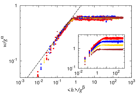
Figure 1: (color online). One-parameter scaling of the standard deviation of the width of the front as a function of the average position of the front as the front moves forward from some initial (rough) configuration. The main figure shows data collapse for $\alpha=\beta=4/7$, and the inset shows the same data with no scaling, i.e. $\alpha=\beta=0$. The straight line has slope $288/637\approx 0.45$ — see text. The data are extracted from simulations with, from top-down in the inset, $g\in(0.05,0.1,0.2,0.5)$. Each group in the inset is comprised of data from systems of sizes 64-256 with constant $E/L$.

We now assume that the front width obeys Family-Vicsek scaling fv85 , i.e.,

$$w(L,\langle h\rangle)=L^{\zeta}\ f\left(\frac{\langle h\rangle}{L^{\kappa}}\right)\;,$$ (6)

where

$$f(q)=\left\{\begin{array}[]{l l}q^{\zeta/\kappa}&\quad\text{if $q\to 0$\;, }\\ constant&\quad\text{if $q\to\infty$\;.}\\ \end{array}\right.$$ (7)

For $\langle h\rangle\ll L^{\kappa}$, and assuming that we are dealing with ordinary percolation, we may relate $\langle h\rangle$ to the number of fibers below and including the front, $A$, by the fractal dimension $D_{A}=91/48$ sa92 , $\langle h\rangle^{D_{A}}\sim A$. Invoking Mandelbrot’s area-perimeter relation, we may also relate the length of the front, $l$ to the number of fibers below and including the front, $l\sim A^{D_{h}/2}$, where $D_{h}=7/4$ gr05 ; m77 . Eliminating $A$ between these two expressions leads to $l\sim\langle h\rangle^{D_{H}D_{A}/2}$. We relate the length of the front $l$ to its width $w$ by the relation $l\sim w^{D_{H}}(L/w)$ gsh13 . Eliminating $l$ between these two relations gives

$$w\sim\langle h\rangle^{D_{A}D_{H}/(2D_{H}-2)}=\langle h\rangle^{288/637}\;,$$ (8)

where $288/637\approx 0.45$. The straight line in Fig. 1 has this slope. We may now calculate the dynamical exponent $\kappa$ in Eq. (6). We find $\kappa=637/432\approx 1.47$.

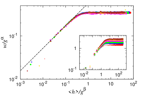
Figure 2: (color online). One-parameter scaling of $w$ as a function of $\langle h\rangle$ with $g$ as the scaling parameter. The main figure shows data collapse for $\alpha=\beta=0.4$. The inset shows unscaled data, i.e. $\alpha=\beta=0$. The slope of the straight line is $0.52$. The parameter values are, from top-down in the inset, $g\in(0.007,0.008,0.01,0.015,0.02,0.03)$. The system size is $L=64$.

Fig. 2 shows the corresponding one-parameter scaling as in Fig. 1, but now for systems with a much lower $e=7.8\times 10^{-4}$, placing us in the realm of the fluctuating line model gsh13 . The two scaling exponents that produce data collapse are $\alpha=\beta=0.4$. By a least squares fit, we determine $w\sim\langle h\rangle^{0.52\pm 0.05}$. This value is very close to the one seen for large $e$ values, and consistent with the measurement of Tallakstad et al. ttssm11 , who found $0.55$ and Schmittbuhl et al. sdm01-1 who found $0.52$, both groups using sintered PMMA plates.

Assuming Family-Vicsek scaling, we determine the dynamical exponent to be $\kappa=0.75\pm 0.07$. This is consistent with the value reported by Duemmer and Krauth for the fluctuating line model, $\kappa=0.70\pm 0.5$.

The dynamical exponent reported by Måloy and Schmittbuhl ms01 for the PMMA system was $\kappa=1.2$. We find $\kappa=1.47$ on small scales and $\kappa=0.75$ on large scales.

It was observed by Santucci et al. sgtshm10 that the large-scale roughness regime shows a gaussian distribution of the height fluctuations, whereas in the small-scale it broadens to a non-gaussian distribution. We investigate this in our model. We define the height fluctuations as $\Delta h(1)=|h_{i+1}(n)-h_{i}(n)|$. By changing the elastic constant, $E$ in our model while keeping the step size constant, the result is equivalent to changing the step size in the experiment. We show in Fig. 3 the distribution of fluctuations for different $E$. We see that for soft systems, the distribution is gaussian. As the system stiffens, the distribution broadens as in the experiment.

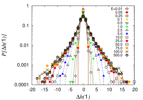
Figure 3: (color online). Histogram of height fluctuations with respect to $\Delta h(1)=|h_{i+1}(n)-h_{i}(n)|$ for different elastic constants. The distribution follows a gaussian when the system is soft and broadens when the system stiffens.

IV Local velocity distribution

We examine the distribution of local velocities using the waiting time matrix (WTM) method msst06 . The WTM method consists of letting the fracture move across a matrix with all elements equal to zero in discrete time steps. Every time step, the matrix elements that contain the front are incremented by one. When the front has passed, the matrix contains the time the front spent in each position. Hence, matrix elements contaning low values correspond to rapid front movements and large values correspond to slow, pinned movement. From the WTM, one can then calculate the spatiotemporal map of velocities by mapping the coordinates of the front at each step in the simulation onto the local velocities $V(x,y)$ calculated from the inverse of the waiting time, thus obtaining $v(x,t)$. From this map we then calculate the global average velocity $\langle v\rangle$ and the distribution of local velocities $P(v)$. It has been found experimentally that this distribution follows

$$P(v/\langle v\rangle)\sim(v/\langle v\rangle)^{-\eta},\quad\textrm{for}\quad v/\langle v\rangle>1,$$ (9)

with the exponent $\eta=2.55\pm 0.15$ msst06 ; ttssm11 . The results from our simulations are shown in Fig. 4 for scaled elastic constant $e=1.6\times 10^{-4}$ and $7.8\times 10^{-4}$. The slope in the figure is obtained through a linear fit and has the value $2.53$. Based on this figure, we follow Tallakstad et al. ttssm11 and define a pinning regime where $v<\langle v\rangle$ and a depinning regime where $v>\langle v\rangle$.

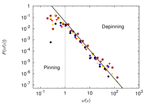
Figure 4: (color online). Distribution of local velocities scaled by the global average velocity. Results are based on simulations of sizes $L=64,128$ with $e=1.56\times 10^{-4},7.81\times 10^{-4}$, respectively, and loading gradient in the range $g\in[0.01-0.05]$. A fit to the data for $v>\langle v\rangle$ yields a power law behavior with an exponent of $-2.53$.

IV.1 Space and time correlations

From the local velocities, we calculate the normalized correlation functions in space, $G(\Delta x)$, and time, $G(\Delta t)$

$$G(\Delta x) =\left\langle\frac{\langle[v(x+\Delta x,t)-\langle v\rangle_{x}][v(x,t)-\langle v\rangle_{x}]\rangle}{\sigma_{x}^{2}}\right\rangle_{t}\;,$$ (10a)

$$G(\Delta t) =\left\langle\frac{\langle[v(x,t+\Delta t)-\langle v\rangle_{t}][v(x,t)-\langle v\rangle_{t}]\rangle}{\sigma_{t}^{2}}\right\rangle_{x}\;.$$ (10b)

$\sigma_{x/t}$ and $\langle\phantom{v}\rangle_{x/t}$ denote standard deviation and average over $x$ or $t$. The results for $G(\Delta x)$ is presented in figure 5. The results are in qualitative agreement with what has been reported experimentally ttssm11 . Due to the small system sizes available numerically, the cutoff we observe is extremely sharp. Still, the data appears to be consistent with a power law distribution with an exponential cutoff $G(\Delta x)=A(\Delta x/L)^{-\tau_{x}}\textrm{exp}(-\Delta x/0.1L)$ with $\tau_{x}=0.4$. This is in the same range as the values reported by Tallakstad et al. ttssm11 , where $\tau_{x}=0.53\pm 0.12$.

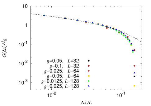
Figure 5: (color online). Spatial correlation function $G(\Delta x)$. Data collapse is obtained when $\Delta x$ is scaled with the system size and $G(\Delta x)$ is scaled with $\sqrt{g}$. The line is a fit to a power law with exponential cutoff $G(\Delta x)=A(\Delta x/L)^{-\tau_{x}}\textrm{exp}(-\Delta x/0.1L)$ with $\tau_{x}=0.4$. The parameters used are as in Fig. 4.

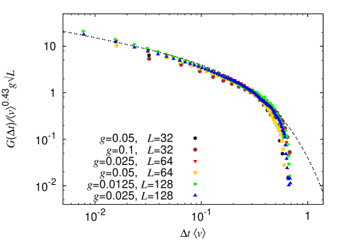
Figure 6: (color online). Temporal correlation function. Best data collapse is obtained when scaling $\Delta t$ by $1/\langle v\rangle$ and $G(\Delta t)$ by $\langle v\rangle^{0.43}g\sqrt{L}$. The line is a fit to a power law with exponential cutoff $G(\Delta t)=B(\Delta t\langle v\rangle)^{-\tau_{t}}\textrm{exp}(-\Delta t\langle v\rangle/0.25)$ with $\tau_{t}=0.43$. The parameters used are as in Fig. 4.

In figure 6, we show the results of the analysis of the temporal velocity distribution. Again, we attempt to fit the data to a power law with exponential cutoff, $G(\Delta t)=B(\Delta t\langle v\rangle)^{-\tau_{t}}\textrm{exp}(-\Delta t\langle v\rangle/0.25)$, with exponent $\tau_{t}=0.43$. The scaling resemble closely that observed by Tallakstad et al. ttssm11 .

We note that data collapse is obtained in Fig. 5 when the correlation function is scaled by $g^{1/2}$ and $\Delta x$ by $L$, and in Fig. 6, the correlation function is scaled by $gL^{1/2}$.

V Cluster analysis

In the following we analyze the geometrical structure of the areas swept by the crack front during avalanches.

Following Tallakstad et al. ttssm11 , we construct thresholded velocity maps $V_{C}$ in such a way that

$$V_{C}=\begin{cases}1,&\mbox{for }v\geq C\langle v\rangle\\ 0,&\mbox{for }v<C\langle v\rangle\end{cases}\;,$$ (11)

in the depinning regime and

$$V_{C}=\begin{cases}1,&\mbox{for }v\leq\langle v\rangle/C\\ 0,&\mbox{for }v>\langle v\rangle/C\end{cases}\;,$$ (12)

in the pinning regime. $C$ is a constant in the range of $2-12$ for depinning and $1.5-6$ for pinning for our simulations. For larger system sizes, larger $C$ are possible. Examples of these matrices are shown in figure 7, where the structural difference between depinning and pinning clusters can be seen. In the spirit of de Saint-Exupéry we may characterize the pinning clusters as snakelike, whereas the depinning clusters are elephant-in-snakelike e43 . The following analysis uses only $L=64$ and $L=128$, and are based on 250 and 100 samples, respectively. $g=0.025$ for the smaller systems, and $g=0.0125$ for the larger systems. For $L=64$, $e=1.6\times 10^{-4}$, and for $L=128$, $e=7.8\times 10^{-4}$. The systems will for these $e$-values behave virtually identical gsh13 .

Depinning         Pinning
C=2           C=1.5

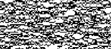
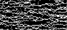
C=4           C=3

C=10           C=5

Figure 7: Part of the thresholded velocity matrix showing depinning clusters on the left and pinning clusters on the right. The images are from a system of size $L=128$, $g=0.0125$ and $e=7.8\times 10^{-4}$. White areas are areas where the local velocities are either above C$\langle v\rangle$ (depinning) or below $\frac{1}{\textrm{C}}\langle v\rangle$ (pinning).

V.1 Size distribution of clusters

We denote the number of bonds in a cluster the size or area of a cluster $S$. Both experiments msst06 ; ttssm11 and numerical simulations using the fluctuating line model bsp08 on in-plane fracture, show a power law distribution $P(S)\sim S^{-\gamma}$ for $S$ with exponent close to $\gamma=1.56$ ttssm11 or $\gamma=1.65$ bsp08 .

We show in Fig. 8 the probability distribution of $S$ both for pinning and depinning for scaled elastic constant $e=1.6\times 10^{-4}$. Our data are consistent with previous measurements, but due to the limited size of the numerical simulations currently available, the exponent cannot be accurately determined. One prominent feature of the clusters is that due to the small system size, the presence of large clusters for low values of $C$ suppresses the number of smaller clusters, and for high values of $C$, the number of large clusters is reduced by the filtering process in $C$. This is a pure finite size effect, which we assume will disappear for larger system sizes. The experiments, which would correspond to a very large simulation size, shows no such dependence on $C$. A direct comparison between the experimental and our data is given in Figure 9.

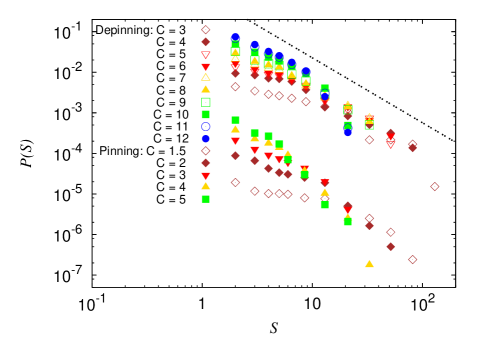
Figure 8: (color online). Probability distribution function of the size of clusters, $S$, for a range of $C$ values for both pinning (lower cluster of points) and depinning clusters (upper cluster of points). The data for pinning clusters are shifted down by 0.005 to visually separate the two regimes. The slope of the line is $\gamma=1.6$. $L=64$, $e=1.6\times 10^{-4}$.

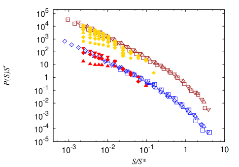
Figure 9: (color online). Size distribution of clusters. Depinning clusters on top and pinning clusters below. The longest data series (unfilled markers) are experimental data obtained with permission from the authors ttssm11 . The shorter data series (filled markers) are numerical data from Fig. 8. The experimental data are unchanged from ttssm11 , so $S^{\prime}=S^{*\gamma}$ and $S^{*}$ are as given in ttssm11 . Due to lack of direct physical parameter comparison, the numerical data are scaled to match the experimental data to verify similar behavior.

V.2 Aspect ratio of clusters

Next, we extract the linear extensions as length and height from the cluster sizes. This is done by enclosing each cluster in a bounding box of size $l_{x}$ by $l_{y}$. Although the appearance differs greatly between pinning and depinning clusters, the method for determining $l_{x}$ and $l_{y}$ are the same. As seen qualitatively in Fig. 7, pinning clusters are much longer than they are wide, and in a worst-case scenario they could approximate the diagonal in the bounding box, which would lead to a gross over-estimation of $l_{y}$. However, such behavior was not seen for $L=64,128$ and we judge the approximation of $l_{y}$ to be equally sound in both regimes.

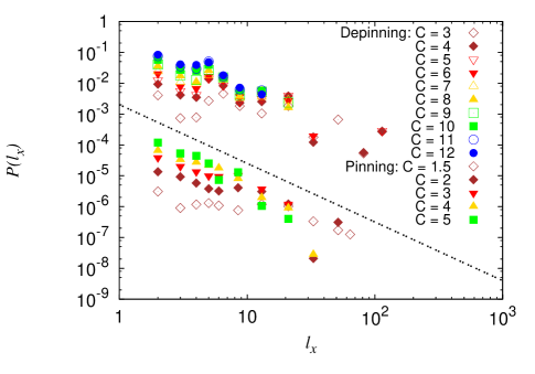
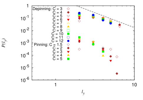
Figure 10: (color online). Probability distribution function of the linear extension of the clusters both parallel and perpendicular to the fracture front. The data for pinning clusters are shifted down for visual clarity by 0.001 for $l_{x}$ and 0.005 for $l_{y}$. The slope of the line in the top figure is $\beta_{x}=1.9$ and in the bottom figure $\beta_{y}=2.4$.

Figure 10 shows the size distributions of $l_{x}$ and $l_{y}$ for scaled elastic constant $e=1.6\times 10^{-4}$. As in Fig. 8, there is a pronounced dependence on $C$. The data indicate power law distributions $P(l_{x})\sim l_{x}^{-\beta_{x}}$ and $P(l_{y})\sim l_{y}^{-\beta_{y}}$ ttssm11 . The data are plotted with lines showing values of the exponents equal to the experimentally obtained $\beta_{x}=1.93$ and $\beta_{y}=2.36$ ttssm11 . Both pinning and depinning data show behaviour consistent with the experimental data.

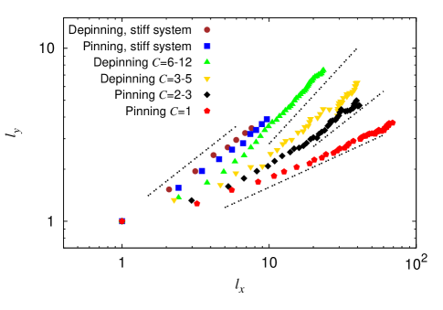
Figure 11: (color online). Local scaling of the clusters. The lines are guides to the eye, but the slopes are based on linear regression and the values are in descending order 0.91, 0.67, 0.67, and 0.39. The data labeled stiff system are from simulations using a Young’s modulus four orders of magnitude greater than what is used in the rest of the simulations. $L=128$, $g=0.0125$, and $e=7.8\times 10^{-4}$ and $e=7.8$. Further details in the text.

Turning to examine the relation between $l_{y}$ and $l_{x}$, we plot these against each other in Fig. 11. This data is more well-behaved than the probability distributions, so scaling relations are more pronounced. The data are consistent with a relation of type

$$l_{y}\sim l_{x}^{H}\;,$$ (13)

as studied both by Tallakstad et al. ttssm11 and Bonamy et al. bsp08 in respectively the experimental system and with the fluctuating line model.

We see a clear dependency of $H$ on parameters such as $e$ and $C$. Considering the depinning case first for $e=7.8\times 10^{-4}$, we divide the data between $C^{\textrm{high}}\in[6-12]$, a group containing data from only the highest local velocities, and $C^{\textrm{low}}\in[3-5]$, containing lower local velocities. There is a clear visual difference in behavior between the two groups: The group with the higher $C$ values, have the higher slope. We measure the corresponding exponents to be $H_{\textrm{d}}^{\textrm{high}}=0.9$ and $H_{\textrm{d}}^{\textrm{low}}=0.65$.

In the pinning regime we similarly divide between low and high local velocity effects, except that the range of available $C$ is much smaller, so we find $C^{\textrm{high}}=2,3$ and $C^{\textrm{low}}=1$. This yields the two exponents $H_{\textrm{p}}^{\textrm{high}}=0.65$ and $H_{\textrm{p}}^{\textrm{low}}=0.4$.

It has been suggested that $H$ is another measure of $\zeta$, the roughness exponent msst06 ; bsp08 ; lsz10 . In order to test this, we have added data both for pinning and depinning of a stiff system ($e=7.8$) in Fig. 11. If the conjecture is right in this case, we would expect a $H$ exponent equal to $2/3$. We have added such slopes, and indeed this seems fulfilled.

We may then speculate whether the exponents that we measure for the softer system ($e=7.8\times 10^{-4}$), indeed are roughness exponents — at least for some groups of $C$ values.

Another way to examine these scaling relations is to check the relation between $l_{x},l_{y}$ and $S$. We expect to see a power law relationship of type

$$l_{i}\sim S^{\alpha_{i}}\;.$$ (14)

The data are plotted in Fig. 12, in which data for the highest local velocities are not included, $C=C^{\textrm{low}}$ for both pinning and depinning. In the depinning regime, we find the exponents $\alpha_{x}^{\textrm{d}}=0.6$ and $\alpha_{y}^{\textrm{d}}=0.4$. Eliminating $S$, we get a measure of $H$ through

$$l_{y}\sim l_{x}^{\alpha_{y}/\alpha_{x}}=l_{x}^{H}\;,$$ (15)

resulting in $H_{\textrm{d}}=0.65$. In the pinning regime we find $\alpha_{x}^{\textrm{p}}=0.75$ and $\alpha_{y}^{\textrm{p}}=0.3$, yielding $H_{\textrm{p}}=0.4$.

These results are to be compared to the experimental measurements ttssm11 giving $\alpha_{x}=0.62\pm 0.04$ in pinning and the depinning regime and $\alpha_{y}=0.41\pm 0.06$ or $0.34\pm 0.05$ in the depinning regime depending on how the bounding box was defined. This leads to the value $H=\alpha_{y}/\alpha_{x}=0.66$ or 0.55 depending on the bounding box used. Bonamy et al. bsp08 found $H=0.65\pm 0.05$.

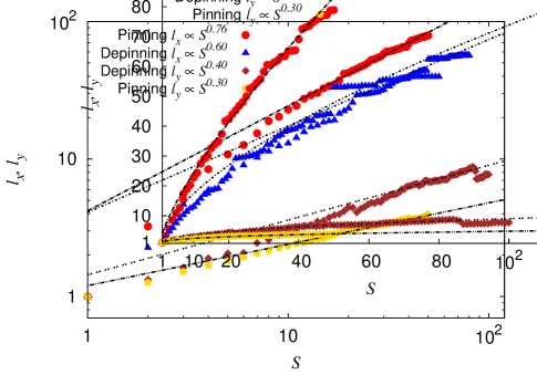
Figure 12: (color online). Linear size of both pinning and depinning clusters as a function of cluster size. The simulation parameters are the same as for Fig. 11.

VI Discussion

In our model, $e$ and $g$ are the most important input parameters. $g$ effectively controls the loading conditions. A high value for $g$ amounts to a large angle of contact between the materials, or slow loading conditions, and vice versa. As long as $1/g$ is in a range where it allows the front to develop but not extend out of the system, we see no change in any scaling exponents we have investigated. This behavior is supported by the experimental results where no dependence on the loading conditions was found and the average propagation velocity of the front spanned more than four and a half orders of magnitude ttssm11 .

The parameter $e$ controls the material behavior. A small value for $e$ can amount to model a system of low modulus of elasticity or a long length scale, and vice versa. Based on the behavior alluded to in our model, we may propose the following scenario. For low values of $e$, the fracture process is due to stress concentration leading to damage forming on the fracture front. This regime is classified by a roughness exponent of $\zeta_{\textrm{large}}=0.39$ and an underlying burst process of same exponent $H=\zeta_{\textrm{large}}$. As $e$ increases, the burst process changes behavior to $H=\zeta_{\textrm{small}}=0.67$, while the front is still characterized by $\zeta_{\textrm{large}}$. As $e$ is increased further, the effect of the burst exponent begins to show on the scale of the front and damage begins to form ahead of the front. At this point, the roughness exponent changes from 0.39 and grows into 0.67. At higher $e$, both the burst process and the roughness of the front is now characterized by the larger exponent $H=\zeta_{\textrm{small}}=0.67$.

VII Conclusion

We have developed a minimal model which we have previously shown to contain two different fracture growth processes which reproduce results from experiments with fracture fronts of roughness $\zeta_{\textrm{small}}=0.67$ on small length scales and $\zeta_{\textrm{large}}=0.39$ on larger length scales gsh13 . In this paper we have shown that this quasistatic model also produces data consistent with the experimental analysis of the dynamics of the fracture front. Most notably we recover the existence and behavior of a depinning and a pinning regime. In the pinning regime we recover the same 0.39-scaling exponent of the front in the bursts. In the depinning regime we can see traces of this behavior, but more importantly, we recover the 0.67-scaling exponent of the front seen on shorter length scales. From this, we conjecture that the collective behavior of the underlying bond breaking process is first and most visible in the damage bursts. The global front roughness changes according to the change in burst process when one process suppresses the other, i.e., on a different scale.

References

- [1] B. r. Lawn, Fracture of Brittle Solids, 2nd Ed. (Cambridge Univ. Press, Cambridge, 1993).
- [2] J. Schmittbuhl, S. Roux, J.-P. Vilotte and K. J. Måløy, Phys. Rev. Lett. 74 1787 (1995).
- [3] J. Schmittbuhl and K. J. Måløy, Phys. Rev. Lett. 78 3888 (1997).
- [4] S. Ramanathan, D. Ertas and D. S. Fisher, Phys. Rev. Lett. 79, 873 (1997).
- [5] A. Delaplace, J. Schmittbuhl and K. J. Måløy, Phys. Rev. E. 60 1337 (1999).
- [6] A. Rosso and W. Krauth, Phys. Rev. E. 65 R025101 (2002).
- [7] J. Schmittbuhl, A. Hansen and G. G. Batrouni, Phys. Rev. Lett. 90 045505 (2003).
- [8] S. Santucci, M. Grob, R. Toussaint, J. Schmittbuhl, A. Hansen and K. J. Måløy, Europhys. Lett. 92 44001 (2010).
- [9] D. Bonamy, J. Appl. Phys. D, 42, 214014 (2009).
- [10] D. Bonamy and E. Bouchaud, Phys. Rep. 498 1 (2011).
- [11] K. J. Måløy and J. Schmittbuhl, Phys. Rev. Lett. 87, 105502 (2001).
- [12] K. J. Måløy, S. Santucci, J. Schmittbuhl and R. Toussaint, Phys. Rev. Lett. 96, 045501 (2006).
- [13] K. T. Tallakstad, R. Toussaint, S. Santucci, J. Schmittbuhl and K. J. Måløy, Phys. Rev. E, 83, 046108 (2011).
- [14] O. Lengliné, R. Toussaint, J. Schmittbuhl, J. E. Elkhoury, J. P. Ampuero, K. T. Tallakstad, S. Santucci and K. J. Måløy, Phys. Rev. E, 84, 036104 (2011).
- [15] J. P. Bouchaud, E. Bouchaud, G. Lapasset and J. Planès, Phys. Rev. Lett. 71 2240 (1993).
- [16] L. Laurson, S. Santucci and S. Zapperi, Phys. Rev. E, 81, 046116 (2010).
- [17] E. Bouchaud, J. P. Bouchaud, D. S. Fisher, S. Ramanathan and J. R. Rice, J. Mech. Phys. Sol. 50, 1703 (2002).
- [18] G. G. Batrouni, A. Hansen and J. Schmittbuhl, Phys. Rev. E. 65 036126 (2002).
- [19] K. S. Gjerden, A. Stormo and A. Hansen, J. Phys: Conf. Series, 402, 012039 (2012).
- [20] K. S. Gjerden, A. Stormo and A. Hansen, arXiv:1301.2174 (2013).
- [21] A. Hansen, G. G. Batrouni, T. Ramstad and J. Schmittbuhl, Phys. Rev. E. 75 030102 (2007).
- [22] D. Bonamy, S. Santucci and L. Ponson, Phys. Rev. Lett. 101, 045501 (2008).
- [23] J. Sethna, K. Dahmen and C. Myers, Nature, 410, 242 (2001).
- [24] A. R. Mehrabi, H. Rassamdana, and M. Sahimi, Phys. Rev. E 56 712 (1997).
- [25] I. Simonsen, A. Hansen and O. M. Nes, Phys. Rev. E 58 2779 (1998).
- [26] S. Pradhan, A. Hansen and B. K. Chakrabarti, Rev. Mod. Phys. 82, 499 (2010).
- [27] K. L. Johnson, Contact Mechanics (Cambridge University Press, Cambridge, 1985).
- [28] G. G. Batrouni, A. Hansen and M. Nelkin, Phys. Rev. Lett. 57, 1336 (1986).
- [29] G. G. Batrouni and A. Hansen, J. Stat. Phys. 52, 747 (1988).
- [30] A. Stormo, K. S. Gjerden and A. Hansen, Phys. Rev. E, 86, R025101 (2012).
- [31] A. Hansen, Comp. Sci. Engn. 7, (5), 90 (2005).
- [32] B. Sapoval, M. Rosso and J. -F. Gouyet, J. Phys. Lett. 46, L149 (1985).
- [33] J.-F. Gouyet and M. Rosso, Physica A 357 86 (2005).
- [34] A. Delaplace, S. Roux and G. Pijaudier-Cabot, J. Engn. Mech. 127 646 (2001).
- [35] F. Family and T. Vicsek, J. Phys. A 18, L75 (1985).
- [36] D. Stauffer and A. Aharony, Introduction to percolation theory (Francis and Taylor, London, 1992).
- [37] B. B. Mandelbrot, Fractal forms, chance and dimensions (W. H. Freeman, San Francisco, 1977).
- [38] J. Schmittbuhl, A. Delaplace and K. J. Måløy in E. Bouchaud et al. (Eds.) Physical Aspects of Fracture (Kluwer Acad. Publ., Amsterdam, 2001).
- [39] O. Duemmer and W. Krauth, J. Stat. Phys. P01019 (2007).
- [40] A. de Saint-Exupéry, Le Petit Prince (Éditions Gallimard, Paris, 1943).