Constraints on the source of ultra-high energy cosmic rays using anisotropy vs chemical composition

Abstract

The joint analysis of anisotropy signals and chemical composition of ultra-high energy cosmic rays offers strong potential for shedding light on the sources of these particles. Following up on an earlier idea, this paper studies the anisotropies produced by protons of energy $>E/Z$, assuming that anisotropies at energy $>E$ have been produced by nuclei of charge $Z$, which share the same magnetic rigidity. We calculate the number of secondary protons produced through photodisintegration of the primary heavy nuclei. Making the extreme assumption that the source does not inject any proton, we find that the source(s) responsible for anisotropies such as reported by the Pierre Auger Observatory should lie closer than $\sim$20-30, 80-100 and 180-200 Mpc if the anisotropy signal is mainly composed of oxygen, silicon and iron nuclei respectively. A violation of this constraint would otherwise result in the secondary protons forming a more significant anisotropy signal at lower energies. Even if the source were located closer than this distance, it would require an extraordinary metallicity $\gtrsim 120,1600,1100$ times solar metallicity in the acceleration zone of the source, for oxygen, silicon and iron respectively, to ensure that the concomitantly injected protons not to produce a more significant low energy anisotropy. This offers interesting prospects for constraining the nature and the source of ultra-high energy cosmic rays with the increase in statistics expected from next generation detectors.

1 Introduction

The origin of ultra–high energy cosmic rays (UHECRs) is a long–standing puzzle of high energy astrophysics and astroparticle physics. It is commonly believed that the source of these particles with energy $\gtrsim 10^{19}\,$eV are powerful extragalactic astrophysical objects. The candidates include active galactic nuclei (AGN, e.g, Biermann & Strittmatter 1987; Takahara 1990; Rachen & Biermann 1993; Berezinsky et al. 2006; Dermer et al. 2009), gamma–ray bursts (GRBs, e.g., Waxman 1995; Vietri 1995; Dermer & Atoyan 2006; Murase & Nagataki 2006), semi–relativistic hypernova (e.g. Wang et al., 2007; Budnik et al., 2008; Chakraborti et al., 2011; Liu & Wang, 2012) and extragalactic rotation-powered young pulsars (Arons, 2003; Fang et al., 2012).

On their way to the detector, UHECRs suffer inevitable interactions with the cosmic microwave background (CMB) and the extragalactic background light (EBL) that permeate extragalactic space, in particular Bethe–Heitler pair production, photo-pion production and photodisintegration. Photo-hadronic interactions inevitably introduce a high energy cut–off in the UHECR spectrum beyond $\sim 5\times 10^{19}$eV(Greisen, 1966; Zatsepin & Kuz’min, 1966; Puget et al., 1976) [GZK], due to the rapid decrease of the attenuation length of UHECRs with increasing energy. Above these GZK energies, the typical horizon to which sources can be detected shrinks to values of the order of $\sim 100-200\,$Mpc. This cut–off/suppression feature has now been observed by different experiments at a statistically significant level (Abbasi et al., 2008; The Pierre AUGER Collaboration et al., 2008; Abraham et al., 2010), implying notably that the sources of the highest energy cosmic rays must be nearby luminous objects (e.g. Waxman, 1995, 2005; Farrar & Gruzinov, 2009; Piran, 2010; Taylor et al., 2011).

The Pierre Auger Observatory (PAO), presently the largest UHECR observatory, has reported the detection 69 events within the energy range 55–142 EeV between January 2004 and December 2009 (The Pierre AUGER Collaboration et al., 2010). A detailed analysis has shown that the fraction of these events correlating with nearby AGN ($<75\,$Mpc) in the Véron-Cetty and Véron (VCV) catalog is ($38^{+7}_{-6}$)%, above the isotropic expectation of 21%. Most of this excess is found around the direction of Centaurus A (Cen A) within a surrounding 18^∘ window, in which 13 events in the energy range 55–84 EeV are observed while only 3.2 are expected (The Pierre AUGER Collaboration et al., 2010). However, both the intergalactic and the Galactic magnetic field deflect the trajectories of cosmic rays, resulting in apparent correlations with objects which are not necessarily their true birth places. Furthermore, measurements on the maximum air shower elongations $\langle X_{\rm max}\rangle$ and their rms ($\sigma_{X_{\rm max}}$) by the PAO suggest that the chemical composition of UHECRs are progressively dominated by heavier nuclei at energies above 4 EeV (Abraham et al., 2010). If the cosmic rays are indeed intermediate–mass or heavy nuclei, the deviation of their arrival directions due to propagation in the intervening magnetic fields must be significant, hence the observation of anisotropies appears slightly surprising. From a theoretical point of view, it may appear more favorable to accelerate heavy nuclei, as their higher charge, comparatively to protons, reduce the energetic constraints placed on the source candidates, e.g. Lemoine & Waxman (2009). However, it also requires the acceleration site to be abundant in intermediate–mass or heavy elements, well beyond a typical galactic composition (Pierre Auger Collaboration et al., 2011; Liu et al., 2012). Finally, other experiments, such as HiRes or the Telescope Array, find that the composition at $\gtrsim 10^{19}\,$eV remains dominated by light nuclei (Abbasi et al., 2010; Tsunesada et al., 2011).

One way to make progress is to use the pattern of anisotropies as a function of energy. This idea was first proposed in Lemoine & Waxman (2009): if a source produces an anisotropy signal at energy $E$ with cosmic ray nuclei of charge $Z$, it should also produce a similar anisotropy pattern at energies $E/Z$ via the proton component that is emitted along with the nuclei, given that the trajectory of cosmic rays within a magnetic field is only rigidity–dependent. It is easy to show that the low energy anisotropy should appear stronger, possibly much stronger than the high energy anisotropy (assuming a chemical composition similar to that inferred at the source of Galactic cosmic rays), offering means to constrain the chemical composition of the source. This test has been applied on the Pierre Auger Observatory dataset and no significant anisotropy has been found at energies $E/Z$, with $E=55\,$EeV and $Z=6,14,26$ (Pierre Auger Collaboration et al., 2011).

In the present work, we push further and generalize this idea by considering the amount of secondary protons produced through photodisintegration interactions of the primary nuclei. We provide detailed analytical and numerical estimates of the ratio of significance of the anisotropy at $E/Z$ vs $E$, and derive the maximal distance to the source $D_{\rm max}$ in order to avoid the formation of a stronger anisotropy pattern produced by the secondary protons at energy $E/Z$. This bound does not depend on the amount of protons produced by the source. We also discuss how the comparison of the anisotropy ratio constrains the metal abundance in the source, independently of the injection spectral index, and emphasize how large this metal abundance must be, if the anisotropies persist at high energies, but not at low energies. Finally, we briefly discuss the prospects for the detection of anisotropies at higher energies than $E$, with next generation experiments, based on current reports of anisotropies at $E$.

The layout of this paper is arranged as follows. In § 2, we discuss how the absence of a low–energy anisotropy signal could constrain the source distance and its metal abundance. In §3, we discuss the low energy proton fraction and the possible anisotropy signal at higher energies, as well as their implication for the source. We draw some conclusions in §4.

2 Anisotropies at constant rigidity

2.1 Low energy anisotropy signal

We assume that some anisotropy is detected within a solid angle $\Delta\Omega$ in the energy range from $E_{1}$ to $E_{2}$. Following up on Lemoine & Waxman (2009), we quantify the significance of the anisotropy through its signal–to–noise ratio. Before doing so, we define the injected spectrum of an element with nuclear charge number $Z$ as

$$q_{Z,\rm inj}=k_{Z}E^{-s}\ ,$$ (1)

with $s$ the power law index and $k_{Z}$ the relative abundance of this element at a given energy. Provided that the maximum energy $E_{Z,\rm max}$ and the minimum energy $E_{Z,\rm min}$ of the accelerated spectrum are proportional to $Z$, i.e. scale with rigidity, the total mass of the element of charge $Z$ and mass $A_{Z}$ scales as

$$M_{Z}\propto A_{Z}\int q_{Z,\rm inj}dE\propto k_{Z}A_{Z}Z^{1-s}\ .$$ (2)

Note that the above result does not depend on the magnitude of $s$, and the missing prefactor does not depend on $Z$. This implies in particular that the ratio of the relative abundance of a species at a given energy to that of hydrogen takes the form

$$\frac{k_{Z}}{k_{p}}\,=\,Z^{s-1}A_{Z}^{-1}\frac{M_{Z}}{M_{\rm H}}.$$ (3)

We then denote respectively the number of injected and propagated primary cosmic rays with nuclear charge $Z$ in the energy range $[E_{1},E_{2}]$ by $N_{Z,\rm inj}(E_{1};E_{2})$ and $N_{Z,\rm prop}(E_{1};E_{2})$. These two quantities are related through

$$N_{Z,\rm prop}(E_{1};E_{2})=f_{Z,\rm surv}(E_{1};E_{2})N_{Z,\rm inj}(E_{1};E_{2}),$$ (4)

where

$$f_{Z,\rm surv}(E_{1};E_{2})\,\equiv\,\frac{\int_{E_{1}}^{E_{2}}q_{Z,\rm prop}(E)\,{\rm d}E}{\int_{E_{1}}^{E_{2}}q_{Z,\rm inj}(E)\,{\rm d}E}$$ (5)

is the surviving fraction of primaries after propagation.

As we do not know the precise composition of cosmic ray events constituting the anisotropy signal, in a first scenario (A) we regard the fragments with less than $Z/4$ lost nucleons as primaries ( i.e., $q_{Z,\rm prop}=\sum\limits_{i=3/4Z}^{Z}q_{i,\rm prop}$). This ad-hoc choice guarantees that all arriving nuclei in the energy range $[E_{1},E_{2}]$ which have suffered at most $Z/4$ photodisintegration interactions retain a similar rigidity, and thus follow a similar path in the intervening magnetic fields. Lighter nuclei, i.e. those that have suffered more than $Z/4$ interactions and arrive in $[E_{1},E_{2}]$ carry higher rigidity. Depending on the intervening magnetic fields, such cosmic rays may or may not contribute to the anisotropies, since the magnetic fields may form a blurred image centered on the source (with higher rigidity cosmic rays clustering closer to the source direction), or impart a systematic shift in the arrival directions, in which case the higher rigidity particles might lie outside $\Delta\Omega$, e.g. Waxman & Miralda-Escudé (1996); Kotera & Lemoine (2008). To account for this uncertainty, we will consider in the following an alternative scenario (B), in which $E_{2}\rightarrow+\infty$ and as many photodisintegration interactions are allowed ( i.e., $q_{Z,\rm prop}=\sum\limits_{i=2}^{Z}q_{i,\rm prop}$), provided the nucleus arrives with energy $>E_{1}$. In this scenario (B), we thus sum up over all rigidities in excess of $E_{1}/Z$.

We adopt the premise that anisotropy in the arrival distribution of UHECR nuclei has been detected at high energies between $E_{1}$ and $E_{2}$, ie. at energies of the order of the GZK energy. Since protons with the same rigidity have energies between $E_{1}/Z$ to $E_{2}/Z$, one may safely neglect their subsequent energy losses given that their loss lengths at these energies are of the order of $\sim 1\,$Gpc, considerably larger than the source distance considered here ($\lesssim 100\,$Mpc). Photodisintegration interactions of nuclei with energy in the range $(A_{Z}/Z)[E_{1},E_{2}]\,\approx\,[2E_{1},2E_{2}]$ produce secondary protons with energy in the range $[E_{1}/Z,E_{2}/Z]$, with number

$$N_{p,\rm dis}(E_{1}/Z;E_{2}/Z)\,=\,A_{Z}f_{Z,\rm loss}(2E_{1};2E_{2})N_{Z,\rm inj}(2E_{1};2E_{2})\,=\,2^{1-s}A_{Z}f_{Z,\rm loss}(2E_{1};2E_{2})N_{Z,\rm inj}(E_{1};E_{2})\ ,$$ (6)

where

$$f_{Z,\rm loss}(2E_{1};2E_{2})\,\equiv\,\frac{\int_{E_{1}/Z}^{E_{2}/Z}\,q_{p,\rm dis}\,{\rm d}E}{A_{Z}\int_{2E_{1}}^{2E_{2}}q_{Z,\rm inj}\,{\rm d}E}\ .$$ (7)

In this expression, $q_{p,\rm dis}$ represents the spectrum of secondary protons produced during propagation.

At low energies, the primary protons also contribute to the anisotropy, with

$$N_{p,\rm prop}(E_{1}/Z;E_{2}/Z)\,\simeq\,N_{p,\rm inj}(E_{1}/Z;E_{2}/Z)\,=\,\frac{M_{\rm H}}{M_{Z}}A_{Z}N_{Z,\rm inj}(E_{1};E_{2})\ .$$ (8)

Note that the last equality is of particular interest. It shows that $N_{p,\rm prop}(E_{1}/Z;E_{2}/Z)/N_{Z,\rm inj}(E_{1};E_{2})=(M_{H}/M_{Z})A_{Z}$ controls the scaling of the signal-to-noise ratio of the low energy to high energy anisotropy signals. This scaling factor does not depend on the injection spectrum index, but does depend on the metal abundance at the source. It remains valid for general injection spectra, provided this spectrum is shaped by rigidity, i.e. $q_{Z,\rm inj}(E)\propto\phi(E/Z)$, with $\phi$ an arbitrary function.

The noise is given by the square root of number of events expected from the averaged all-sky spectrum of UHECRs in the same solid angle $\Delta\Omega$. The observed spectrum of the isotropic background can be approximately described by a broken power law beyond $\sim 10^{18}$ eV (The Pierre AUGER Collaboration et al., 2010), i.e.,

$$\frac{{\rm d}N_{\rm iso}}{{\rm d}E}\bigg{|}_{\rm iso}=N_{0}\times\left\{\begin{array}[]{ll}\left(E/E_{b}\right)^{-p_{1}}&E<E_{\rm b},\\ \left(E/E_{b}\right)^{-p_{2}}&E\geq E_{\rm b}\end{array}\right.$$ (9)

where $p_{1}=2.6$, $p_{2}=4.3$ and $E_{\rm b}=10^{19.46}$eV. $N_{0}$ represents the overall amplitude, which cancels out in the following calculation. The noise counts in the energy range $[E_{1},E_{2}]$ then reads

$$N_{\rm iso}(E_{1};E_{2})\,=\,\Delta\Omega\int_{E_{1}}^{E_{2}}\frac{{\rm d}N_{\rm iso}}{{\rm d}E}\,{\rm d}E$$ (10)

and for the low energy noise we have

$$N_{\rm iso}(E_{1}/Z;E_{2}/Z)\,=\,\Delta\Omega\int_{E_{1}/Z}^{E_{2}/Z}\frac{{\rm d}N_{\rm iso}}{{\rm d}E}\,{\rm d}E=\eta Z^{p_{1}-1}N_{\rm iso}(E_{1};E_{2})\ ,$$ (11)

with $\eta\equiv(1-p_{2})(1-p_{1})^{-1}\left(E_{2}^{1-p_{1}}-E_{1}^{1-p_{1}}\right)\left(E_{2}^{1-p_{2}}-E_{1}^{1-p_{2}}\right)^{-1}E_{\rm b}^{p_{1}-p_{2}}$. The above equation is valid for $E_{1}>E_{b}$ and $E_{2}/Z<E_{b}$, which is the case of the ”Cen A excess”. If $E_{2}<E_{b}$ or $E_{1}/Z>E_{b}$, Eq. (11) will read $Z^{p_{1}-1}N_{\rm iso}(E_{1};E_{2})$ or $Z^{p_{2}-1}N_{\rm iso}(E_{1};E_{2})$ respectively.

Assuming the anisotropy is mainly caused by cosmic ray nuclei with charge $Z$, the signal-to-noise ratio in the energy range $[E_{1},E_{2}]$ can then be expressed as

$$\Sigma_{Z}(E_{1};E_{2})\,=\,\frac{N_{Z,\rm prop}(E_{1};E_{2})}{\sqrt{N_{\rm iso}(E_{1};E_{2})}}=\frac{f_{Z,\rm surv}(E_{1};E_{2})N_{Z,\rm inj}(E_{1};E_{2})}{\sqrt{N_{\rm iso}(E_{1};E_{2})}},$$ (12)

while the S/N of the low energy anisotropy produced by protons with the same rigidity is

$$\Sigma_{p}(E_{1}/Z;E_{2}/Z)\,=\,\frac{N_{p,\rm prop}(E_{1}/Z;E_{2}/Z)+N_{p,\rm dis}(E_{1}/Z;E_{2}/Z)}{\sqrt{N_{\rm iso}(E_{1}/Z;E_{2}/Z)}}\,=\,\frac{A_{Z}\left[M_{\rm H}/M_{Z}\,+\,2^{1-s}f_{Z,\rm loss}(2E_{1};2E_{2})\right]N_{Z,\rm inj}(E_{1};E_{2})}{\sqrt{\eta Z^{p_{1}-1}N_{\rm iso}(E_{1};E_{2})}}\ .$$ (13)

Consequently, the ratio of the signal-to-noise ratios at low to high energy reads

$$\frac{\Sigma_{p}}{\Sigma_{Z}}=\frac{2M_{H}/M_{Z}\,+\,2^{2-s}f_{Z,\rm loss}(2E_{1};2E_{2})}{f_{Z,\rm surv}(E_{1};E_{2})\sqrt{\eta Z^{p_{1}-3}}}\ ,$$ (14)

and if no anisotropy is recorded at low energies, one requires $\Sigma_{p}/\Sigma_{Z}<1$. For reference, the Pierre Auger Observatory data indicate that, for the Cen A excess, $\Sigma_{p}/\Sigma_{Z}\,\lesssim\,(2.,1.8,0.8)$ at the 95% c.l., for $Z=6,14,26$ corresponding to carbon, silicon and iron Pierre Auger Collaboration et al. (2011). The exact number depends on the statistics (which of course have increased since this analysis was carried out), and on the elements adopted in the analysis. In the following, we use the constraint $\Sigma_{p}/\Sigma_{Z}<1$ to impose a limit on the maximum source distance.

In terms of the (inverse) metal abundance, this constraint can be rewritten

$$\frac{M_{\rm H}}{M_{Z}}<\frac{1}{2}\left[\sqrt{\eta Z^{p_{1}-3}}f_{Z,\rm surv}(E_{1};E_{2})-2^{2-s}f_{Z,\rm loss}(2E_{1};2E_{2})\right]\ .$$ (15)

Again, if secondary protons are ignored, meaning $f_{Z,\rm loss}(2E_{1};2E_{2})\rightarrow 0$ in the above, then the non-detection of anisotropy at low energies imposes a lower limit of $M_{Z}/M_{\rm H}$ which does not depend on the spectral index. Note that this statement is not in contradiction with the statement in the Pierre Auger Collaboration et al. (2011), that the limit on the quantity $f_{p}/f_{Z}$ used in that paper depends on the spectral index. This is due to the fact that $f_{p}/f_{Z}$, which is defined at a given energy, is not the ”proton to heavy fraction in the source” or the ”relative proton abundance”, as it is misleadingly referred to in the Auger paper (in the notation of that paper, the relative proton abundance is $k_{p}/k_{Z}$, which is equivalent to our $M_{p}/M_{Z}$).

The minimum required metallicity of the element responsible for the observed anisotropy thus depends on the value of $f_{Z,\rm surv}$ and $f_{Z,\rm loss}$, which are directly determined by the source distance. A larger source distance will result in a smaller $f_{Z,\rm surv}$ and a larger $f_{Z,\rm loss}$ as more nuclei are photodisintegrated. There exists therefore a critical distance, beyond which the abundance of hydrogen in the source relative to metals becomes negative. This happens when $f_{Z,\rm loss}(2E_{1};2E_{2})/f_{Z,\rm surv.}(E_{1};E_{2})\geq 2^{s-2}\sqrt{\eta Z^{p_{1}-3}}$, meaning that even if the source injects no primary protons, secondary protons produced during propagation cause a stronger anisotropy at low energies. Therefore, the critical distance, which we denote by $D_{\rm max}$ hereafter, is the upper limit of the distance of the source responsible for the anisotropy signal in $[E_{1},E_{2}]$. The value of $D_{\rm max}$ is also related to the primary cosmic ray species adopted and the injection spectrum used. Once these parameters are given, we can uniquely determine $D_{\rm max}$ by finding the distance for which $\Sigma_{p}(E_{1}/Z;E_{2}/Z)/\Sigma_{Z}(E_{1};E_{2})=1$ using the method outlined above.

2.2 Photodisintegration of nuclei

Ultra-high energy cosmic rays interact with the CMB and EBL photons while they propagate through extragalactic space. For nuclei, energy losses due to the photodisintegration process and the Bethe–Heitler process (pair production) by CMB photons are comparable around 55 EeV. As energy increases, the photodisintegration process plays a more and more dominant role in the energy loss process. Photodisintegration does not change the Lorentz factor of the cosmic ray nucleus, but does lead to the nucleus losing one or several nucleons as well as $\alpha$ particles through the giant dipole resonance (GDR) or quasi–deuteron (QD) process. These secondary nuclei can be further disintegrated to protons. On average, the mass number of a nucleus evolves as Stecker (1969)

$$-\frac{{\rm d}A}{{\rm d}x}\,=\,\frac{1}{2\gamma_{A}^{2}}\sum_{i}\Delta A_{i}\int_{\epsilon_{{\rm th},i}}^{\infty}{\rm d}\epsilon\,\sigma_{{\rm dis},i}^{A}(\epsilon)\epsilon\,\int_{\epsilon/2\gamma_{A}}^{2\gamma_{A}\epsilon}{\rm d}\epsilon_{\gamma}\,\frac{n_{\gamma}(\epsilon_{\gamma},z)}{\epsilon_{\gamma}^{2}}$$ (16)

with $\sigma_{{\rm dis},i}^{A}$ the cross-section for photodisintegration through the $i$th channel (e.g., single–nucleon emission, deuterium emission, $\alpha$ particle emission and so on), and $\epsilon_{{\rm th},i}$ the threshold energy of the $i$th channel, which is $\sim 10-20\,$MeV for all species of nuclei for the GDR process and $\sim 30\,$MeV for the QD process. $\Delta A_{i}$ is the number of nucleon lost through the $i$th channel (e.g., $\Delta A=1,2,4$ for single nucleon emission, deuteron and $\alpha$ particle emission and so on). $\epsilon_{\gamma}$ and $n_{\gamma}(\epsilon_{\gamma},z)$ are respectively the photon energy and the number density of the target photon field in the lab frame at redshift $z$ while $\epsilon$ is the photon energy in the rest frame of the nucleus. The physics of UHE nuclei transport through the radiation backgrounds has been discussed by a number of authors, e.g. Puget et al. (1976); Bertone et al. (2002); Khan et al. (2005); Hooper et al. (2008); Aloisio et al. (2012). In this work, we will adopt the tabulated cross-section data generated by the code TALYS and implement them into the Monte–Carlo framework along with other energy loss processes, as described in Hooper et al. (2007), to obtain the propagated spectra.

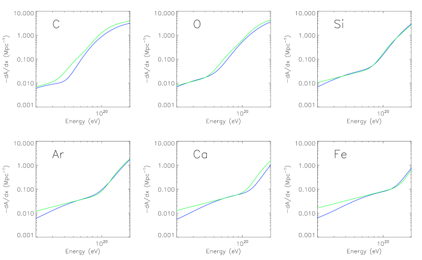
Figure 1: The phenomenological fit of nucleon loss rate for some species of cosmic rays. The blue lines are numerically calculated results while the green ones are plotted based on the analytical expressions (Eq. 17).

As Monte Carlo simulations of nuclei propagation remain somewhat costly in computing, it is useful to have a simple analytical estimate of the photodisintegration process. Detailed treatments are discussed in Hooper et al. (2008); Aloisio et al. (2013a, b). Here, we adopt an even simpler approximation, which provides a sufficiently reliable approximation for the integrations that follow. In this analytical treatment, only the photodisintegration process is taken into account, with all other energy loss processes being neglected. A phenomenological fit of the nucleon loss rate ${\rm d}A/{\rm d}x$ for a nucleus with initial mass number $A_{0}$ and Lorentz factor $\gamma$:

$$-\frac{{\rm d}A}{{\rm d}x}=c_{1}(\gamma_{10})A^{2}+c_{2}(\gamma_{10})A~{}~{}\rm Mpc^{-1}$$ (17)

where $c_{1}(\gamma_{10})$ and $c_{2}(\gamma_{10})$ are functions of the Lorentz factor of cosmic ray nuclei in unit of $10^{10}$, which can be written in the form of $a_{1}\gamma_{10}+a_{2}{\rm exp}(-a_{3}/\gamma_{10}^{a_{4}})$.

Table 1: The best-fit parameters for nucleon loss rate through a MCMC method.

	$c_{1}$	$c_{2}$
$a_{1}$	$9.99\times 10^{-5}$	$2.11\times 10^{-3}$
$a_{2}$	$7.43\times 10^{-3}$	$0.31$
$a_{3}$	$0.69$	1.15
$a_{4}$	$1.79$	2.80

Table 1 presents the results from a Markov Chain Monte Carlo exploration of the parameter space and Fig. 1 shows the phenomenologically fit and numerical nucleon loss rate respectively for several cosmic ray species. From Eq. (17) we can derive the average mass number of a nucleus of initial mass number $A_{0}$ and Lorentz factor $\gamma_{10}$ after propagation over a distance $x$:

$$A(x,\gamma_{10})=\frac{A_{0}c_{2}e^{-c_{2}x}}{A_{0}c_{1}(1-e^{-c_{2}x})+c_{2}}\ .$$ (18)

For Poisson statistics with mean rate ${\rm d}A/{\rm d}x$, the probability that a nucleus undergoes at most $N$ interactions reads

$$P_{N}(A_{Z},x,E)\,\equiv\,\frac{\Gamma\left[N+1,x\,|{\rm d}A/{\rm d}x|\right]}{\Gamma\left[N+1\right]}.$$ (19)

Strictly speaking, Eq. (17) leads to modified Poisson statistics, because the rate ${\rm d}A/{\rm d}x$ depends on $A$, which evolves as photodisintegration interactions occur. It is possible to derive the generalized probability law for $P_{N}$, at the expense of tedious calculation; however, as we demonstrate in the following, the above form for $P_{N}$ provides a sufficient approximation for our case of interest.

One may then derive the propagated spectra, surviving fractions and secondary proton spectra used in the previous subsection, as follows. Consider first the simpler scenario (B) in which one sums up over all fragments with rigidities in excess of $E_{1}/Z$. Writing $Q_{Z,\rm prop}(E)=E\,q_{Z,\rm prop}(E)$ the number of particles per log interval, and neglecting losses other than photodisintegration, one finds

$$Q_{Z,\rm prop}(E)\,=\,\sum_{i=0}^{i=A_{Z}-1}\,p_{i}\left(A_{Z},x,\frac{E}{1-i/A_{Z}}\right)Q_{Z,\rm inj}\left(\frac{E}{1-i/A_{Z}}\right)\ ,$$ (20)

with $p_{i}(A_{Z},x,E)\,\equiv\,\left(x\,|{\rm d}A/{\rm d}x|\right)^{i}\exp\left(-x\,|{\rm d}A/{\rm d}x|\right)/i!$ the probability to undergo $i$ photodisintegration interactions over a distance $x$, thereby decreasing the injection energy from $E/(1-i/A_{Z})$ down to $E$.

Then, the fraction of surviving fragments with rigidity $>E_{1}/Z$ can be obtained as

$$f_{Z,\rm surv}(>E_{1})\,=\,\frac{1}{\int_{E_{1}}^{+\infty}\,q_{Z,\rm inj}(E)dE}\,\int_{\ln E_{1}}^{+\infty}{\rm d}\ln E\,Q_{Z,\rm prop}(E)\,=\,\frac{1}{\int_{E_{1}}^{+\infty}\,q_{Z,\rm inj}(E)dE}\,\int_{E_{1}}^{+\infty}{\rm d}E\,q_{Z,\rm inj}(E)\,P_{j}(A_{Z},x,E)\ ,$$ (21)

with $j\,\equiv\,{\rm min}\left\{A_{Z}-1,{\rm Int}[A_{Z}\left(1-E_{1}/E\right)]\right\}$. The latter equality is obtained by inverting the summation interval between the integral and the discrete sum, changing variables in the integration from $E\rightarrow E/(1-i/A)$, then permuting the order of integration. Note that $P_{j}(A_{Z},x,E)=\sum_{i=0}^{j}p_{i}(A_{Z},x,E)$.

The fraction of photodisintegrated nuclei with energy more than $2E$ is given by $f_{Z,\rm loss}(>2E)=1-f_{Z,\rm surv}(>2E)$, and the number of secondary protons is easily evaluated using Eq. (6).

In Scenario (A), one considers only the fragments with energy in the range $[E_{1},E_{2}]$, which have suffered at most $Z/4$ photodisintegration interactions, so as to study a group of nuclei with similar rigidities. Eq. (20) remains valid, if the sum over $i$ runs from $i=0$ to $i=Z/4$, therefore one finds

$$f_{Z,\rm surv}(E_{1};E_{2})\,=\,\frac{1}{\int_{E_{1}}^{E_{2}}\,q_{Z,\rm inj}(E)\,{\rm d}E}\left\{\int_{E_{1}}^{+\infty}dEq_{Z,\rm inj}(E)\,P_{j_{1}}(A_{Z},x,E)-\int_{E_{2}}^{+\infty}dEq_{Z,\rm inj}(E)\,P_{j_{2}}(A_{Z},x,E)\right\}\ ,$$ (22)

with $j_{1}={\rm min}\left\{Z/4,{\rm int}[A\left(1-E_{1}/E\right)]\right\}$, $j_{2}={\rm min}\left\{Z/4,{\rm int}[A\left(1-E_{2}/E\right)]\right\}$. Here as well, one defines $f_{Z,\rm loss}(>2E)=1-f_{Z,\rm surv}(>2E)$, and the number of secondary protons is easily evaluated using Eq. (6).

2.3 Results

So far, our treatment has remained quite general. Here, we apply it to the specific case of the ”Cen A excess” reported by the Pierre Auger collaboration. We thus use $E_{1}=55\,$EeV, $E_{2}=84\,$EeV and assume for simplicity that the source injects a pure oxygen, silicon or iron composition. In Fig. 2 we show both the analytical and the numerical results of the ratio of anisotropy significance at low to high energies as a function of the distance to the source that is responsible for the anisotropy. In this figure, we do not assume any proton component in the source composition, so that $N_{p,\rm prop}\rightarrow 0$, $M_{\rm H}/M_{Z}\rightarrow 0$ in Eqs. (13) and (14). We adopt an exponential cut–off power law spectrum, as generally expected, with a cut–off energy $E_{\rm max}\propto Z$. The four panels correspond to different injection spectral indices and maximal energies. As can be seen, these results share the following common features.

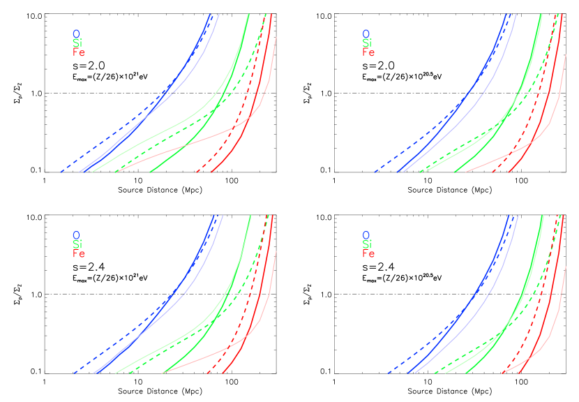
Figure 2: Ratio of anisotropy significance at low to high energies as a function of the distance to the sources responsible for the anisotropy. Solid lines represent the numerical results while dashed lines represent the analytical results; thick solid line: scenario (A), in which one sums up over fragments of similar rigidity, in interval $[E_{1},E_{2}]$, with at most $Z/4$ photodisintegration interactions; thin solid lines: scenario (B), in which one sums up over all fragments with rigidities in excess of $E_{1}/Z$. The source is assumed to inject pure O, Si or Fe composition as indicated.

At small source distances, the anisotropy signal produced by secondary protons is less prominent than the high energy one, because only a few primary nuclei photodisintegrate on this short path length. As more and more secondary protons are produced with increasing source distance, this ratio grows and eventually exceeds unity. In the case $s=2,E_{\rm max}=(Z/26)\times 10^{21}\,$eV, both the analytical treatment and the numerical treatment result in a maximum source distance of $\sim 15$ Mpc, $\sim 60$ Mpc and $\sim 180\,$Mpc for oxygen nuclei, silicon nuclei and iron nuclei respectively. Note that for $E_{\rm max}=(Z/26)\times 10^{21}\,$eV, the source produces protons of energy $\gtrsim 40\,$EeV: such protons would presumably produce a strong anisotropy, though its magnitude would depend strongly on the distribution and characteristics of intervening magnetic fields. We show therefore the case with a high $E_{\rm max}$ for the sake of generality in order to illustrate the dependence of the results on the maximal energy.

From lighter to heavier nuclei, the constraint on the source distance becomes weaker, since at a given energy lighter nuclei carry a comparatively larger Lorentz factor, and as a consequence, their energy lies further beyond the photodisintegration interaction threshold (see also Fig. 1). The small differences of $D_{\rm max}$ for the same species among the four panels can be interpreted as follows: protons at $E/Z$ all come from primary nuclei at $2E$, so a smaller cut–off energy or a steeper power-law slope will decrease the amount of primary nuclei at $2E$, leading to less secondary protons produced at $E/Z$, so that the values of maximum source distances in these cases are larger.

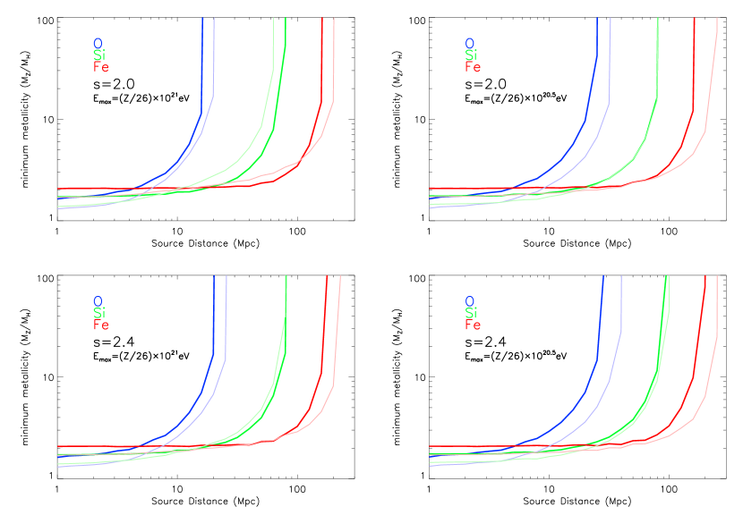
Figure 3: The minimum metal mass relative to hydrogen in the source, assuming pure O, Si or Fe compositions are injected. Thick solid lines and thin solid lines respectively represent results in scenario (A) and (B), which are the same as in Fig. 2.

Another way to plot these results is to consider the minimum metal abundance $M_{Z}/M_{\rm H}$ that is required at the source in order to satisfy the bound $\Sigma_{p}/\Sigma_{Z}<1$. The results are shown in Fig. 3 as a function of the distance to the source. All four panels indicate that the mass ratio of nuclei to proton $\gtrsim 1:1$ is needed. Of course, as the distance increases, so does the minimum $M_{Z}/M_{\rm H}$, in order to compensate for the greater number of secondary protons produced during propagation. The distance where $M_{Z}/M_{H}\rightarrow+\infty$ corresponds to $D_{\rm max}$. Conversely, the asymptote as $D\rightarrow 0$ indicate the minimum $M_{Z}/M_{\rm H}$ amount when secondary protons can be safely neglected.

3 Discussion

We emphasize the method that we have presented remains quite general and could be applied to datasets of next generation experiments. Nevertheless, the results obtained in Figs. 2,3 assume tacitly that the heavy chemical composition and the anisotropy signal reported by the PAO are not artifacts. It is fair to say that these two results remain disputed. The significance level of the anisotropy, for instance, is not comfortably high, and deserves to be improved with extended datasets. The measurements of the chemical composition by the High Resolution Fly’s Eye Experiment (HiRes) and Telescope Array (TA) differ appreciably from that of the PAO. In particular, their data of $\langle X_{\rm max}\rangle$ and rms $\sigma_{X_{\rm max}}$ show a proton dominated spectrum at all energies $>10^{18}\,$eV(Abbasi et al., 2010; Tsunesada et al., 2011). One should not expect to detect anisotropies at low energies if the composition were pure proton, as the low energy protons have a much smaller rigidity than the high energy ones. On the other hand, the analysis of the chemical composition depends on the details of the hadronic interaction model, such as the cross sections, multiplicities and so on. The fact that these parameters are poorly constrained at present prevents one from drawing firm conclusions. As for the apparent anisotropy, Clay et al. (2010) has shown that there is no significant difference between the energy distribution of the events inside and outside the $25^{\circ}$ window of Cen A using a K-S test, implying events around Cen A do not have any special origin; such an analysis cannot provide however a conclusive answer, given the limited event statistics presently available. Additionally, two recent papers suggest that at most 5–6 of events around Cen A can originate from it by backtracing the events’ trajectories in the intervening magnetic field (Farrar et al., 2012; Sushchov et al., 2012). We should, however, be cautious with such strong conclusions given that they depend on the magnetic field model adopted, which still carries a large degree of uncertainty.

3.1 Source metallicity

With the above caveats in mind, it is interesting to discuss where the previous results lead us. The constraints derived from Fig. 3 are indeed quite strong. For reference, the solar composition (Lodders & Palme, 2009) corresponds to $M_{\rm H}/M_{\rm CNO}\,\sim\,70$, $M_{\rm H}/M_{\rm Si}\,\sim\,900$ and $M_{\rm H}/M_{\rm Fe}\,\sim\,550$. Consequently, the minimum metallicities required to match $\Sigma_{p}/\Sigma_{Z}<1$, notwithstanding the secondary protons, are $\sim 120Z_{\odot}$ for CNO, $\sim 1600Z_{\odot}$ for Si and $\sim 1100Z_{\odot}$ for iron like nuclei. The comparison to $Z_{\odot}$ is less severe for oxygen, but this nucleus is also more fragile and the minimum metallicity diverges rapidly beyond some $20-30\,$Mpc. Conversely, the production of secondary protons is less severe for iron nuclei, but for such nuclei, the minimum requirements on the source metallicity are already quite extraordinary.

The observables $\langle X_{\rm max}\rangle$ and $\sigma_{X_{\rm max}}$, as reported by the Pierre Auger Observatory, suggest that the all-sky-averaged composition of arriving UHECRs may be oxygen–like (Hooper & Taylor, 2010). If the anisotropy signal observed by the PAO mainly consists of oxygen–like nuclei, our calculations indicate that the source responsible for the anisotropy should lie within $20-30\,$Mpc. There are only a limited number of known powerful radio-galaxies within this distance, such as Cen A, M87. Such radio-galaxies are relatively weak, in terms of jet power and magnetic luminosity, which implies that they cannot accelerate particles beyond $E_{\rm max}\,\sim Z\times 10^{18}-10^{19}\,$eV, see the discussion in Lemoine & Waxman (2009). Even assuming that these sources accelerate oxygen nuclei to the highest energies, the minimum metallicity required by the above arguments lies well above what is measured in the central parts of such radio-galaxies (Hamann & Ferland, 1999). The situation becomes even worse if one considers silicon or heavier nuclei. Consequently, and as already emphasized in Lemoine & Waxman (2009), the current dataset of the Pierre Auger Observatory, in particular the clustering towards Cen A, does not provide support for acceleration of UHECRs in this object.

If future datasets confirm the existence of anisotropies at high energies, and the absence of anisotropies at low energies, then the present work provides strong constraints on the nature and the source of ultra-high energy cosmic rays: either protons exist at ultra-high energies, and some of them are responsible for the observed anisotropies (in which case no anisotropy is indeed expected at lower energies); or, a close-by source with rather extraordinarily high metallicity produces these anisotropies. The only physically motivated scenario for such a source so far is acceleration at the external shock of a semi-relativistic hypernovae inside the wind of the progenitor (Wang et al., 2007; Budnik et al., 2008; Chakraborti et al., 2011; Liu & Wang, 2012).

3.2 Composition close to the ankle

Provided the same source population produces both UHECRs with energy $>E_{1}$ and $>E_{1}/Z$, the proton fraction at $E_{1}/Z$ becomes an interesting aspect of the problem. The key point indeed is that if $M_{Z}\,\gtrsim\,M_{\rm H}$ inside the sources, as suggested by the above discussion, and all sources are alike, then the chemical composition at $E_{1}/Z$ must contain a significant heavy component. More specifically, the fraction of protons at low energies is given by

$$x_{p}(E_{1}/Z;E_{2}/Z)=\frac{\tilde{N}_{p}(E_{1}/Z;E_{2}/Z)}{\tilde{N}_{Z,\rm prop}(E_{1}/Z;E_{2}/Z)+\tilde{N}_{p}(E_{1}/Z;E_{2}/Z)}$$ (23)

where $\tilde{N}_{p}=\tilde{N}_{p,\rm prop}+\tilde{N}_{p,\rm dis}$ is the total proton number, including the contribution from secondary protons and primary protons, as integrated over all sources, and similarly for $\tilde{N}_{Z,\rm prop}$. Here we neglect the partially disintegrated fragments. Assuming every source has equal emissivity and the same injection spectrum, we have

$$\tilde{N}_{Z,\rm prop}(E_{1};E_{2})\,\simeq\,\int_{(1+z)E_{1}/Z}^{(1+z)E_{2}/Z}q_{Z,\rm inj}(E)\,{\rm d}E\,\int_{0}^{l_{Z,\rm loss}(E)}n(z)f_{Z,\rm surv}(E)\,{\rm d}D_{\rm c}(z)$$ (24)

and

$$\tilde{N}_{p,\rm dis}(E_{1};E_{2})\,\simeq\,A_{Z}\int_{2(1+z)E_{1}}^{2(1+z)E_{2}}q_{Z,\rm inj}(E)\,{\rm d}E\int_{0}^{l_{p,\rm loss}(E/A_{Z})}n(z)f_{Z,\rm loss}(E)\,{\rm d}D_{\rm c}(z).$$ (25)

Here $n(z)$ is the source density as a function of redshift $z$ and $D_{\rm c}(z)$ is the comoving distance to the light cone at redshift $z$; $l_{Z,\rm loss}$ and $l_{p,\rm loss}$ represent the energy loss lengths $\left|E/(dE/dx)\right|$ for nuclei and protons respectively. The second equation assumes that photodisintegration takes place on short distance scales compared to $l_{p,\rm loss}(E/A_{Z})$, which is a very good approximation. The energy losses to be considered here includes all processes besides photodisintegration, such as pair production, adiabatic cooling etc. Since the energy loss distance of protons with energy $(1+z)E/Z$ is much larger than the energy loss distance of nuclei at energy $2(1+z)E$, $f_{Z,\rm loss}\left[2(1+z)E\right]\rightarrow 1$ for most sources. On the other hand, $f_{Z,\rm surv.}\left[(1+z)E/Z\right]\,\approx\,\exp\left\{-D_{\rm c}/l_{Z,\rm loss}\left[(1+z)E/Z)\right]\right\}$ and given that $l_{Z,\rm loss}\left[(1+z)E/Z\right]$ is the upper limit of integration, we have $e^{-1}\lesssim f_{Z,\rm surv.}\lesssim 1$. As an estimation here we take $f_{Z,\rm surv.}=1$. Then, the above two equations can be written as

$$\tilde{N}_{Z,\rm prop}(E_{1};E_{2})\,\approx\,k_{Z}Z^{s-1}\bar{E}^{1-s}\int_{0}^{l_{Z,\rm loss}(\bar{E}/Z)}(1+z)^{1-s}n(z)\,{\rm d}D_{\rm c}$$ (26)

$$\tilde{N}_{p,\rm dis}(E_{1};E_{2})\,\approx\,k_{Z}2^{1-s}\bar{E}^{1-s}A_{Z}\int_{0}^{l_{p,\rm loss}(\bar{E}/Z)}(1+z)^{1-s}n(z)\,{\rm d}D_{\rm c}.$$ (27)

Since $[E_{1},E_{2}]$ is a narrow energy range, we denote the average energy in this range by $\bar{E}$. Considering that $n(z)$ usually evolves with redshift $z$, we make here a further approximation that the term $(1+z)^{1-s}$ cancels the evolution in $n(z)$ to some extent and the integrand is reduced to a constant. Then one can find that

$$x_{p}(E_{1};E_{2})\,\approx\,\frac{1+2^{s-1}M_{H}/M_{Z}}{1+2^{s-1}M_{H}/M_{Z}\,+\,A_{Z}^{s-2}l_{Z,\rm loss}(\bar{E}/Z)/l_{p,\rm loss}(\bar{E}_{\rm thr}/Z)}\ .$$ (28)

In the local Universe, for oxygen nuclei, $[E_{1}/Z,E_{2}/Z]\,\sim\,[7,10]\,$EeV, hence the energy loss in this energy range is comparably caused by photodisintegration on EBL photons and pair production on CMB photons, leading to an energy loss length of $\sim 2-3\,$Gpc. For silicon and iron nuclei, $[E_{1}/Z,E_{2}/Z]\,\sim[4,6]\,$EeV and $[2,3]\,$EeV respectively, in which energy range the dominant cooling process is adiabatic cooling with an energy loss length $\sim 4\,$Gpc. For protons, however, the dominant energy loss process in the corresponding energy range is caused by pair production on CMB photons with an energy loss length $\sim 1-2\,$Gpc. Therefore typically, the energy loss length for nuclei is larger than that for protons by a factor of 2-3. If $2^{s-1}\,M_{\rm H}/M_{Z}\,\lesssim\,1$, as suggested by the previous discussion, this implies in turn that the composition in $[E_{1}/Z,E_{2}/Z]$ should comprise less than $\sim 50\,$% protons, in potential conflict with the claims of a light composition close to the ankle of the cosmic ray spectrum.

Looking at this argument the other way round, the data from the Pierre Auger Observatory shows evidence for the UHECR mass composition becoming progressively heavier at energies $\gtrsim\,$ 4 EeV, while below this energy the same data suggests a proton-like composition. Thus, we should expect $M_{\rm H}/M_{Z}\gtrsim 1$ if the heavy elements at $E_{1}$ are mostly silicon or iron nuclei. In this case, Fig. 3 indicates that one should have detected a secondary anisotropy at the ankle. For oxygen, however, $E_{1}/Z$ already lies in an energy range where the composition apparently departs from proton-like, and the above argument is severely weakened.

3.3 Trans-GZK anisotropies

Another interesting aspect is the possible anisotropy signal that one may expect at higher energies, given the reported anisotropies at $>55\,$EeV. The detection of such anisotropies provides a strong motivation for next generation experiments such as JEM-EUSO (Casolino et al., 2011), which will provide a substantially larger amount of statistics.

Here we start by assuming that the currently observed anisotropy mainly consists of nuclei with charge number $Z$ and that their source also accelerates heavier nuclei with nuclear charge number $Z^{{}^{\prime}}$. These heavier nuclei will produce a similar anisotropy pattern at higher energies $>Z^{\prime}E_{1}/Z$; we define $E_{1}^{\prime}=Z^{\prime}E_{1}/Z$ for clarity. The ratio of significance between these two anisotropy signals then reads

$$\frac{\Sigma_{Z^{\prime}}(>E_{1}^{\prime})}{\Sigma_{Z}(>E_{1})}=\frac{M_{Z^{\prime}}}{M_{Z}}\frac{f_{Z^{\prime},\rm surv.}(>E_{1}^{\prime})}{f_{Z,\rm surv.}(>E_{1})}\left(\frac{Z^{{}^{\prime}}}{Z}\right)^{(p_{2}-3)/2}\ ,$$ (29)

where $f_{Z,\rm surv.}\approx\exp\left(-x/l_{Z,\rm loss}\right)$. With the approximation $A_{Z}\simeq 2Z$, the two species of nuclei with the same rigidity share approximately the same Lorentz factor. At the same Lorentz factor, heavier nuclei lose energy faster than lighter nuclei, but the differences between the energy loss lengths of different species such as O, Si, Fe with rigidity $E/Z$ are at most a factor of a few; furthermore, the energy loss lengths are larger than the maximum source distance $D_{\rm max}$ that we have obtained in Section 3. So we expect $0.1\,\lesssim\,f_{Z^{\prime},\rm surv}(>E_{1}^{\prime})/f_{Z,\rm surv}(>E_{1})\,\lesssim\,1$. Also, $p_{2}=4.3$, hence $\left(Z^{\prime}/Z\right)^{(p_{2}-3)/2}\,\gtrsim\,1$. Therefore, a stronger anisotropy signal is expected at higher energies if the source is more abundant in nuclei $Z^{\prime}$ than nuclei $Z$. In this case, however, some accompanying effects will occur and one should also check whether these effects already cause violations against current measurements or lead to self-contradiction. We consider here the following three aspects.

• secondary protons produced by nuclei $Z^{\prime}$ above energy $E_{1}/Z$. Since nuclei $Z^{\prime}$ at $E_{1}^{\prime}$ have the same rigidity as the nuclei $Z$ at $E_{1}$, the secondary protons emitted by nuclei $Z^{\prime}$ will fall well within the energy range of interest. According to Eq. (6), we can write the secondary protons above $E_{1}/Z$ as $N_{p,\rm dis}(>E_{1}/Z)=A_{Z}f_{Z,\rm loss}(>2E_{1})N_{Z,\rm inj}(>2E_{1})$. As such, we obtain the ratio between the number of secondary protons produced by nuclei $Z^{{}^{\prime}}$ and $Z$ above $E_{1}/Z$

  $$\frac{N_{p^{\prime},\rm dis}}{N_{p,\rm dis}}=\frac{M_{Z^{\prime}}}{M_{Z}}\frac{f_{Z^{\prime},\rm loss}(>2E_{1}^{\prime})}{f_{Z,\rm loss}(>2E_{1})}$$ (30)

  As was discussed above, the energy loss length of nuclei $Z^{\prime}$ is a bit larger than that of nuclei $Z$ with the same Lorentz factor, so $f_{Z^{\prime},\rm loss}(>2E_{1}^{\prime})\,\gtrsim\,f_{Z,\rm loss}(>2E_{1})$. If the source is more abundant in nuclei $Z^{\prime}$ than nuclei $Z$, i.e, $M_{Z^{\prime}}>M_{Z}$, nuclei $Z^{\prime}$ will actually produce more secondary protons than nuclei $Z$, above energy $E_{1}/Z$. As such, when we calculate the low energy proton anisotropy significance, we should also consider the contribution from nuclei $Z^{\prime}$ and add a non–trivial term to the numerator of Eq. (13). Consequently, the maximum source distance derived previously would be further reduced.

• the chemical composition of UHECRs at energy $E_{1}^{\prime}$: as the UHECR background decreases rapidly with increasing energy, the composition of cosmic rays emitted by the source can strongly influence the composition measurement at higher energies, provided the source accelerates a larger fraction of nuclei $Z^{\prime}$ than nuclei $Z$. Although it is difficult to find a quantitative relation between the composition of the source and that of the all–sky averaged composition, one might naively expect that the all–sky averaged composition above a given energy $E$ (denoted as $\xi_{Z}(>E)$) to be positively related to $A_{Z}\frac{N_{Z,\rm prop}(>E)}{N_{\rm iso}(>E)}$, and we find

  $$\frac{\xi_{Z^{\prime}}(>E_{1}^{\prime})}{\xi_{Z}(>E_{1})}=\frac{M_{Z^{\prime}}}{M_{Z}}\frac{f_{Z^{\prime},\rm surv.}(>E_{1}^{\prime})}{f_{Z,\rm surv.}(>E_{1})}\left(\frac{Z^{\prime}}{Z}\right)^{p_{2}-1}=\left(\frac{Z^{\prime}}{Z}\right)^{\frac{p_{2}+1}{2}}\frac{\Sigma_{Z^{\prime}}}{\Sigma_{Z}}$$ (31)

  As one can see, since $Z^{\prime}>Z$, if stronger anisotropy signal is detected at higher energies ($\Sigma_{Z^{\prime}}>\Sigma_{Z}$), the UHECRs composition is expected to be heavier.

• the surviving nuclei $Z^{{}^{\prime}}$ in the energy range between $E_{1}$ and $E_{2}$. Assuming that the source is more abundant in nuclei $Z^{\prime}$ than nuclei $Z$, the source should emit a larger amount of nuclei $Z^{\prime}$ in the energy range $E_{1}$ and $E_{2}$. So after propagation, the number of surviving nuclei in a fixed energy range is $\propto f_{Z,\rm surv.}\int k_{Z}E^{-s}dE\propto f_{Z,\rm surv.}M_{Z}Z^{s-2}$. With the fact that heavier nuclei lose nucleons slower than lighter nuclei at the same energy (not the same Lorentz factor), we expect the ratio of nuclei $Z^{\prime}$ and nuclei $Z$ emitted by the source in the energy range to be

  $$\frac{N_{Z^{\prime},\rm prop}(E_{1};E_{2})}{N_{Z,\rm prop}(E_{1};E_{2})}=\frac{M_{Z^{\prime}}}{M_{Z}}\frac{f_{Z^{\prime},\rm surv.}(E_{1};E_{2})}{f_{Z,\rm surv.}(E_{1};E_{2})}\left(\frac{Z^{\prime}}{Z}\right)^{s-2}>1$$ (32)

  It does not mean however that these $Z^{\prime}$ nuclei would contribute to the anisotropy pattern seen in the range $[E_{1},E_{2}]$, because they have smaller rigidity than the $Z$ nuclei.

If the source does not accelerate nuclei beyond charge $Z$, then the anisotropy at higher energies is produced by nuclei of charge $Z$. To derive the corresponding ratio of significances, make the substitution $M_{Z^{\prime}}/M_{Z}\rightarrow 1$, $Z^{\prime}/Z\rightarrow E_{1}^{\prime}/E_{1}$ in Eq. (29). Then, with $(p_{2}-3)/2\simeq 0.65$, one expects the ratio to increase slightly up to the energy at which the distance to the source matches the energy loss distances, then to drop sharply beyond this distance. The detection of such a feature would provide useful constraints on $Z$ and $D$.

4 Conclusion

In this work, we have generalized a test of the chemical composition of UHECRs, which proposes to use the anisotropy pattern measured as a function of energy. The basic principle is that if anisotropies are observed at high energies $E\sim 6\times 10^{19}\,$eV, and if one assumes that these anisotropies are caused by heavy nuclei of charge $Z$, then one should observe a strong anisotropy signal at energies $E/Z$ close to the ankle, due to the proton component (Lemoine & Waxman, 2009). In the present paper, we have accounted for the production of secondary protons through the photodisintegration interactions of nuclei. Assuming that no anisotropy signal is detected at low energies, we derive an upper bound on the distance to the source.

Our numerical estimates are based on the report of the Pierre Auger Observatory of an excess in the direction to Cen A. At present, the significance of this detection is not well established and one must await future data to confirm or invalidate it. Nevertheless, the method presented here remains general and might well be applied to future more extended datasets. Taking the results of the Pierre Auger Observatory at face value, we derive a maximal distance to the source of order $20-30\,$Mpc, $80-100\,$Mpc, $180-200\,$Mpc if the nuclei responsible for the anisotropies are oxygen, silicon or iron respectively. The differences between these estimates of the maximal distance are directly related to the energy loss lengths of these nuclei at GZK energies. Our results are summarized in Fig. 3, which shows the minimum mass of metals relatively to hydrogen required in the source, in order to produce a weaker anisotropy at $E/Z$ than at $E$. At distances exceeding the above estimates, this amount diverges, meaning that even if the source does not accelerate any protons, the amount of secondary protons produced during propagation is sufficient to cause a secondary anisotropy at $E/Z$ larger than that observed at $E$. At small source distances, where photodisintegration effects are negligible, one nevertheless finds a minimum mass $M_{Z}/M_{\rm H}\,\gtrsim\,1$. When measured relatively to the solar composition, this indicates that the metallicity inside the source should exceed $\sim 120Z_{\odot}$, $\sim 1600Z_{\odot}$, or $\sim 1100Z_{\odot}$ if oxygen, silicon or iron nuclei are responsible for the high energy anisotropy. This result does not depend on the spectral index, or on the details of the injection spectrum, as long as the latter is shaped by rigidity. When combined, these bounds on the distance and metallicity bring in quite stringent constraints on the source of these particles. Additionally, these constraints imply that if the heavy nuclei at GZK energies are silicon or iron, the proton fraction in the all-sky composition at ankle energies should be less than $\sim 50\,$%, in potential conflict with measured data.

References

- Abbasi et al. (2008) Abbasi, R. U., Abu-Zayyad, T., Allen, M., et al. 2008, Physical Review Letters, 100, 101101
- Abbasi et al. (2010) Abbasi, R. U., Abu-Zayyad, T., Al-Seady, M., et al. 2010, Physical Review Letters, 104, 161101
- Abraham et al. (2010) Abraham, J., Abreu, P., Aglietta, M., et al. 2010, Physical Review Letters, 104, 091101
- Abraham et al. (2010) Abraham, J., Abreu, P., Aglietta, M., et al. 2010, Physics Letters B, 685, 239
- Aloisio et al. (2012) Aloisio, R., Boncioli, D., Grillo, A. F., Petrera, S., Salamida, F. 2012, JCAP, 10, 007
- Aloisio et al. (2013a) Aloisio, R., Berezinsky, V., Grigorieva, S. 2013, Astropart. Phys., 41, 73
- Aloisio et al. (2013b) Aloisio, R., Berezinsky, V., Grigorieva, S. 2013, Astropart. Phys., 41, 94
- Arons (2003) Arons, J. 2003, ApJ, 589, 871
- Berezinsky et al. (2006) Berezinsky, V., Gazizov, A., & Grigorieva, S. 2006, Phys. Rev. D, 74, 043005
- Bertone et al. (2002) Bertone, G., Isola, C., Lemoine, M., Sigl, G. 2002, PRD, 66, 103003
- Biermann & Strittmatter (1987) Biermann, P. L., & Strittmatter, P. A. 1987, ApJ, 322, 643
- Budnik et al. (2008) Budnik, R., Katz, B., MacFadyen, A., Waxman E. 2008, ApJ 673, 928
- Casolino et al. (2011) Casolino, M., Adams, J. H., Bertaina, M. E., et al. 2011, Astrophysics and Space Sciences Transactions, 7, 477
- Chakraborti et al. (2011) Chakraborti, S., Ray, A., Soderberg, A. M., Loeb, A., & Chandra, P. 2011, Nature Communications, 2,
- Clay et al. (2010) Clay, R. W., Whelan, B. J., & Edwards, P. G. 2010, Pub. Astron. Soc. Aus., 27, 439
- Dermer & Atoyan (2006) Dermer, C. D., & Atoyan, A. 2006, New Journal of Physics, 8, 122
- Dermer et al. (2009) Dermer, C. D., Razzaque, S., Finke, J. D., & Atoyan, A. 2009, New Journal of Physics, 11, 065016
- Fang et al. (2012) Fang, K., Kotera, K., & Olinto, A. V. 2012, ApJ, 750, 118
- Farrar & Gruzinov (2009) Farrar, G. R., & Gruzinov, A. 2009, ApJ, 693, 329
- Farrar et al. (2012) Farrar, G. R., Jansson, R., Feain, I. J., & Gaensler, B. M. 2012, arXiv:1211.7086
- Greisen (1966) Greisen, K. 1966, Physical Review Letters, 16, 748
- Hamann & Ferland (1999) Hamann, F., & Ferland, G. 1999, ARA&A, 37, 487
- Hooper et al. (2007) Hooper, D., Sarkar, S., & Taylor, A. M. 2007, Astroparticle Physics, 27, 199
- Hooper et al. (2008) Hooper, D., Sarkar, S., & Taylor, A. M. 2008, Phys. Rev. D, 77, 103007
- Hooper & Taylor (2010) Hooper, D., & Taylor, A. M. 2010, Astroparticle Physics, 33, 151
- Khan et al. (2005) Khan, E., Goriely, S., Allard, D., Parizot, E., Suomijärvi, T., Koning, A., Hilaire, S., Duijvestijn, M. C. 2005, Astropart. Phys. 23, 191
- Kotera & Lemoine (2008) Kotera, K., Lemoine, M. 2008, PRD. 77, 123003
- Lemoine & Waxman (2009) Lemoine, M., & Waxman, E. 2009, JCAP, 11, 9
- Liu & Wang (2012) Liu, R.-Y., & Wang, X.-Y. 2012, ApJ, 746, 40
- Liu et al. (2012) Liu, R.-Y., Wang, X.-Y., Wang, W., & Taylor, A. M. 2012, ApJ, 755, 139
- Lodders & Palme (2009) Lodders, K., & Palme, H. 2009, Meteoritics and Planetary Science Supplement, 72, 5154
- Murase & Nagataki (2006) Murase, K., & Nagataki, S. 2006, Phys. Rev. D, 73, 063002
- Puget et al. (1976) Puget, J. L., Stecker, F. W., & Bredekamp, J. H. 1976, ApJ, 205, 638
- Rachen & Biermann (1993) Rachen, J. P., Biermann, P. L. 1993, AA, 272, 161
- Stecker (1969) Stecker, F. W. 1969, Physical Review, 180, 1264
- Sushchov et al. (2012) Sushchov, O., Kobzar, O., Hnatyk, B., & Marchenko, V. 2012, arXiv:1212.1402
- Taylor et al. (2011) Taylor, A. M., Ahlers, M., & Aharonian, F. A. 2011, Phys. Rev. D, 84, 105007
- The Pierre AUGER Collaboration et al. (2008) The Pierre AUGER Collaboration, et al. 2008, Astroparticle Physics, 29, 188
- The Pierre AUGER Collaboration et al. (2010) The Pierre AUGER Collaboration, et al. 2010, Astroparticle Physics, 34, 314
- Pierre Auger Collaboration et al. (2011) Pierre Auger Collaboration, Abreu, P., Aglietta, M., et al. 2011, JCAP, 6, 22
- Piran (2010) Piran, T. 2010, arXiv:1005.3311
- Takahara (1990) Takahara, F. 1990, Prog. Theor. Phys., 83, 1071
- Tsunesada et al. (2011) Tsunesada, Y. for the Telescope Array Collaboration 2011, arXiv:1111.2507
- Vietri (1995) Vietri, M. 1995, ApJ, 453, 883
- Wang et al. (2007) Wang, X.-Y., Razzaque, S., Mészáros, P., & Dai, Z.-G. 2007, Phys. Rev. D, 76, 083009
- Waxman (1995) Waxman, E. 1995, Physical Review Letters, 75, 386
- Waxman & Miralda-Escudé (1996) Waxman, E., Miralda-Escudé 1996, J., Ap, 472, L89
- Waxman (2005) Waxman, E. 2005, Physica Scripta Volume T, 121, 147
- Zatsepin & Kuz’min (1966) Zatsepin, G. T., & Kuz’min, V. A. 1966, Soviet Journal of Experimental and Theoretical Physics Letters, 4, 78