Charge-symmetry breaking forces and isospin mixing in $\bm{{}^{8}{\rm Be}}$

Abstract

We report Green’s function Monte Carlo calculations of isospin-mixing (IM) matrix elements for the $2^{+}$, $1^{+}$, and $3^{+}$ $T$=0,1 pairs of states at 16-19 MeV excitation in ⁸Be. The realistic Argonne $v_{18}$ (AV18) two-nucleon and Illinois-7 three-nucleon potentials are used to generate the nuclear wave functions. Contributions from the full electromagnetic interaction and strong class III charge-symmetry-breaking (CSB) components of the AV18 potential are evaluated. We also examine two theoretically more complete CSB potentials based on rho-omega mixing, tuned to give the same neutron-neutron scattering length as AV18. The contribution of these different CSB potentials to the ³H-³He, ⁷Li-⁷Be, and ⁸Li-⁸B isovector energy differences is evaluated and reasonable agreement with experiment is obtained. Finally, for the ⁸Be IM calculation we add the small class IV CSB terms coming from one-photon, one-pion, and one-rho exchange, as well as rho-omega mixing. The expectation values of the three CSB models vary by up to 20% in the isovector energy differences, but only by 10% or less in the IM matrix element. The total matrix element gives 85–90% of the experimental IM value of -145 keV for the $2^{+}$ doublet, with about two thirds coming from the Coulomb interaction. We also report the IM matrix element to the first $2^{+}$ state at 3 MeV excitation, which is the final state for various tests of the Standard Model for $\beta$-decay.

I Introduction

The ⁸Be nucleus has a unique excitation spectrum among the light nuclei, exhibiting a low-lying rotational band topped by a set of three isospin-mixed doublets. The experimental spectrum exp8-10 for low-lying states in ⁸Be and its isobaric neighbors ⁸Li and ⁸B is shown in Fig. 1. The structure of these nuclei is well understood on the basis of the allowed spatial symmetries and spin-isospin combinations. Realistic nucleon-nucleon forces are strongly attractive in relative $S$ waves, hence the most spatially symmetric states will be the most tightly bound because they maximize the number of $S$-wave pairs W06 . For ⁸Be, the most symmetric states are total isospin $T$=0 with the Young diagram spatial symmetry [44]. In $LS$ coupling the allowed combinations within the $p$-shell are the ${}^{2S+1}L_{J}$ combinations ${}^{1}S_{0}$, ${}^{1}D_{2}$, and ${}^{1}G_{4}$. These are the dominant pieces of the $J^{\pi}$=$0^{+}$ ground-state and the first $2^{+}$ and $4^{+}$ excitations, respectively, as shown in Fig. 1. The ground state is unstable against breakup into two $\alpha$ particles by 0.1 MeV, but is a very narrow (6 eV) resonance, while the two excited states, which have the structure of two $\alpha$ particles rotating about each other, have much larger widths of about 1.5 and 3.5 MeV, respectively.

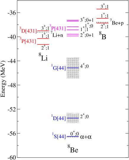
Figure 1: (Color online) Experimental spectrum of $A$=8 nuclei: blue lines are $T$=0 states, red lines are $T$=1 states, and magenta lines are mixed $T$=0+1 states. Dotted lines indicate the thresholds for breakup and shaded areas denote the large widths of the ⁸Be rotational states.

The next highest spatial symmetry states are [431] in character and come in both total isospin $T$=0 and 1 combinations. The $T$=0 states are the spin triplets ${}^{3}P_{0,1,2}$, ${}^{3}D_{1,2,3}$, and ${}^{3}F_{2,3,4}$, while the $T$=1 states come both as these spin triplets and as spin singlets ${}^{1}P_{1}$, ${}^{1}D_{2}$, and ${}^{1}F_{3}$. When diagonalized with a realistic Hamiltonian containing nucleon-nucleon ($N\!N$) and three-nucleon ($3N$) potentials in a microscopic quantum Monte Carlo (QMC) calculation, the first three [431] $T$=0 states are ordered $2^{+}$, $1^{+}$, and $3^{+}$, with about 1 MeV separation, and their dominant components are ${}^{3}P_{2}$, ${}^{3}P_{1}$, and ${}^{3}D_{3}$, respectively WPCP00 . The first three [431] $T$=1 states have the same ordering, and about the same spacing, with the only difference being that there is a moderate amount of ${}^{1}P_{1}$ mixed into the $1^{+}$ state. These $T$=1 states are the isobaric analogs seen in ⁸Li and ⁸B, giving their $2^{+}$ ground states and low-lying $1^{+}$ and $3^{+}$ excited states. The number of $S$-wave $N\!N$ pairs in the [431] symmetry states is the same in both $T$=0 and 1 combinations, so it is reasonable to expect that these states could appear very close to each other in the spectrum of ⁸Be. Experimentally there are two $2^{+}$ states at 16.626 and 16.922 MeV excitation, two $1^{+}$ states at 17.64 and 18.15 MeV, and two $3^{+}$ states at 19.07 and 19.235 MeV, and there is strong experimental evidence for these states being isospin-mixed.

An early detailed analysis of this mixing was given by Barker in the course of making intermediate coupling shell-model calculations for light nuclei Barker66 . The eigenfunctions in his study exhibit the same dominant spatial symmetry components found in the later QMC calculations. A clear experimental signal for isospin mixing of the $2^{+}$ states is that both decay by 2$\alpha$ emission, which is the only particle-decay channel that is energetically allowed, and which is available only through a $T$=0 component in the initial state. Following Barker, the eigenfunctions $\Psi_{a}$, $\Psi_{b}$ of the observed states may be written as linear combinations of the $T$=0 and 1 wave functions:

$$\Psi_{a} = \alpha_{J}\Psi_{0}+\beta_{J}\Psi_{1}\ ,$$

$$\Psi_{b} = \beta_{J}\Psi_{0}-\alpha_{J}\Psi_{1}\ ,$$ (1)

with $\alpha_{J}^{2}+\beta_{J}^{2}=1$. The mixing parameters are related to the ratio of $\alpha$-decay widths:

$$\frac{\Gamma_{a}}{\Gamma_{b}}=\frac{\alpha_{J}^{2}}{\beta_{J}^{2}}\ .$$ (2)

The current experimental values for the widths are $\Gamma_{a}=108.1(5)$ keV and $\Gamma_{b}=74.0(4)$ keV for the 16.626 and 16.922 MeV states, respectively exp8-10 . This implies $\alpha_{2}=0.7705(15)$ and $\beta_{2}=0.6375(19)$.

The eigenenergies $E_{a}$, $E_{b}$ (with $E_{a}<E_{b}$) are given by

$$E_{a,b}=\frac{H_{00}+H_{11}}{2}\pm\sqrt{\left(\frac{H_{00}-H_{11}}{2}\right)^{2}+(H_{01})^{2}}$$ (3)

where $H_{00}$ is the diagonal energy expectation in the pure $T$=0 state, $H_{11}$ is the expectation value in the $T$=1 state, and $H_{01}$ is the off-diagonal isospin-mixing (IM) matrix element that connects $T$=0 and 1. The experimental eigenvalues and eigenenergies, imply that these matrix elements are $H_{00}=16.746(2)$ MeV, $H_{11}=16.802(2)$ MeV, and $H_{01}=-145(3)$ keV. These values are very close to those deduced originally by Barker, and the values of the mixing parameters for the $2^{+}$ states are supported by a variety of other experimental data.

The analysis for the $1^{+}$ and $3^{+}$ doublets is somewhat less direct because multiple decay channels are available. For the $1^{+}$ doublet, Barker used the ratio of $M1$ $\gamma$ transitions from the 17.64 MeV state to the 16.626 and 16.922 MeV $2^{+}$ states, which at the time were in the ratio 1:0.07, to deduce mixing parameters of $\alpha_{1}=0.24$ and $\beta_{1}=0.97$. More recent experiments and analyses by Oothoudt and Garvey OG77 produce slightly less mixing, with $\alpha_{1}=0.21(3)$ corresponding to $H_{01}=-103(14)$ keV. For the $3^{+}$ doublet, Barker examined the ratio of neutron to proton widths for the 19.235 MeV state, and deduced mixing parameters $\alpha_{3}=0.41$, $\beta_{3}=0.91$, and $H_{01}=-63$ keV. However, according to Oothoudt and Garvey, the data is consistent with $0.31<\alpha_{3}<0.52$, corresponding to an IM matrix element ranging from $-47$ to $-71$ keV, and we use this as the empirical value. But Oothoudt and Garvey also find, on the basis of newer experimental data, an even broader range of possible mixing, so the experimental situation for the $3^{+}$ doublet is quite unclear.

The energies of the isospin-unmixed states inferred by using these IM parameters are given in Table 1, along with the experimental energies and the GFMC energies for the AV18+IL7 Hamiltonian discussed below.

Table 1: GFMC ground state energy and excitations in MeV for the AV18+IL7 Hamiltonian compared to the empirical energies of the isospin-unmixed states and the experimental (isospin-mixed) energies of the ⁸Be spectrum; also given are the GFMC point proton (= neutron) radii in fm. Theoretical or experimental errors $\geq 1$ in the last digit are shown in parentheses.

$J^{\pi};T$	GFMC	Empirical	Experiment	$r_{p}$
$0^{+}$	$-56.3(1)$		$-56.50$	$2.40$
$2^{+}$	$+3.2(2)$		$+3.03(1)$	$2.45(1)$
$4^{+}$	$+11.2(3)$		$+11.35(15)$	$2.48(2)$
$2^{+};0$	$+16.8(2)$	$+16.746(3)$	$+16.626(3)$	$2.28$
$2^{+};1$	$+16.8(2)$	$+16.802(3)$	$+16.922(3)$	$2.33$
$1^{+};1$	$+17.5(2)$	$+17.66(1)$	$+17.640(1)$	$2.39$
$1^{+};0$	$+18.0(2)$	$+18.13(1)$	$+18.150(4)$	$2.36$
$3^{+};1$	$+19.4(2)$	$+19.10(3)$	$+19.07(3)$	$2.31$
$3^{+};0$	$+19.9(2)$	$+19.21(2)$	$+19.235(10)$	$2.35$

Barker evaluated the Coulomb contribution to the IM matrix element $H^{C}_{01}$ in all three cases and found it to have the correct negative sign, but only about half the required magnitude Barker66 . A variational Monte Carlo (VMC) evaluation of the mixing using the microscopic Argonne v₁₈ (AV18) nucleon-nucleon interaction, which has additional electromagnetic terms and strong charge-independence breaking, found significant additional contributions to $H_{01}$ WPCP00 . In this paper we carry out more accurate Green’s function Monte Carlo (GFMC) evaluations of these terms, and consider extensions of the charge-independence breaking of the original AV18 model. We also evaluate the mixing matrix element with the first $2^{+}$ state of ⁸Be, which is the final state for the beta-decay of both ⁸Li and ⁸B and a testing ground for weak decay terms beyond the Standard Model.

II Hamiltonian

Charge symmetry implies the invariance of a system under a rotational transformation which reverses the sign of the third component of isospin for all its components, e.g., in nuclei $p\rightarrow n$ and $n\rightarrow p$. The classification of $N\!N$ forces according to their dependence on isospin or charge has been given by Henley and Miller HM79 . The dominant $N\!N$ forces are class I or charge-independent (CI) forces, which may depend on the total isospin of a pair, but not on the charges of the individual nucleons. Thus in a $T$=1 state, a CI force between $pp$, $np$, and $nn$ pairs is identical, while the force for a $T$=0 $np$ pair can be different. A class II force is charge-dependent (CD) but maintains charge symmetry, so in $T$=1 states, a CD force for $pp$ and $nn$ pairs is identical, but different for $np$ pairs. Both class III and class IV potentials violate charge independence and charge symmetry, with a class III charge-symmetry-breaking (CSB) force differentiating between $pp$ and $nn$ pairs, while a class IV force can mix $T$=0 and 1 $np$ pairs. The Coulomb force between two protons can be written as a linear combination of class I, II, and III terms, while the interaction between nucleon magnetic moments involves all four classes. The relative magnitude of these $N\!N$ forces is in the order class I $>$ II $>$ III $>$ IV vKFG96 .

The Hamiltonian used in this work has the form

$$H=\sum_{i}K_{i}+{\sum_{i<j}}v_{ij}+\sum_{i<j<k}V_{ijk}\ ,$$ (4)

where $K_{i}$ is the nonrelativistic kinetic energy and $v_{ij}$ and $V_{ijk}$ are respectively the Argonne $v_{18}$ (AV18) WSS95 and Illinois-7 (IL7) PPWC01 ; P08b potentials. The kinetic energy includes both CI and CSB contributions, the latter coming from the neutron-proton mass difference:

$$K_{i} = K^{\rm CI}_{i}+K^{\rm CSB}_{i}$$

$$= -\frac{\hbar^{2}}{4}(\frac{1}{m_{p}}+\frac{1}{m_{n}})\nabla^{2}_{i}-\frac{\hbar^{2}}{4}(\frac{1}{m_{p}}-\frac{1}{m_{n}})\tau_{iz}\nabla^{2}_{i}\ ,$$

where $\tau_{iz}$ is the third component of isospin for nucleon $i$. The AV18 potential has the structure:

$$v_{ij}=v_{\gamma}(r_{ij})+\sum_{p=1,18}[v^{p}_{\pi}(r_{ij})+v^{p}_{I}(r_{ij})+v^{p}_{S}(r_{ij})]O^{p}_{ij}\ .$$ (6)

Here $v_{\gamma}$ is a complete electromagnetic interaction, including Coulomb, magnetic moment, vacuum polarization, and other terms. The nuclear part of the potential has long-range one-pion-exchange (OPE) $v_{\pi}$, and intermediate $v_{I}$ and short-range $v_{S}$ phenomenological parts. The operators $O^{p}_{ij}$ include fourteen CI terms:

$$O^{p=1,14}_{ij} = [1,\sigma_{i}\cdot\sigma_{j},S_{ij},{\bf L\cdot S},{\bf L}^{2},{\bf L}^{2}(\sigma_{i}\cdot\sigma_{j}),({\bf L\cdot S})^{2}]$$ (7)

$$\otimes [1,\tau_{i}\cdot\tau_{j}]\ ,$$

plus three CD terms and one class III CSB term:

$$O^{p=15,18}_{ij}=[1,\sigma_{i}\cdot\sigma_{j},S_{ij}]\otimes T_{ij}\ ,\ (\tau_{i}+\tau_{j})_{z}\ .$$ (8)

Here $\sigma_{i}$ is the Pauli spin operator for nucleon $i$, $S_{ij}=3(\sigma_{i}\cdot{\hat{r}}_{ij})(\sigma_{j}\cdot{\hat{r}}_{ij})-\sigma_{i}\cdot\sigma_{j}$ is the tensor operator, ${\bf S}=(\sigma_{i}+\sigma_{j})/2$ is the total pair spin, ${\bf L}$ is the pair orbital momentum operator, and $T_{ij}=3\tau_{iz}\tau_{jz}-\tau_{i}\cdot\tau_{j}$ is the isotensor operator.

The long-ranged OPE yields a significant CD term arising from the difference between neutral and charged-pion masses. The intermediate and short-range contributions to the force are constrained by the differences between the considerable amount of $pp$ and $np$ scattering data in the ${}^{1}S_{0}$ channel. Additional charge dependence, such as that arising from a spin-orbit term, might be expected. Extracting such a term would require an independent analysis of $np$ data in ${}^{3}P_{J}$ channels, which has not yet been made available.

The CSB term was determined by a slight alteration of the ${}^{1}S_{0}(pp)$ potential to fit the only available piece of $nn$ scattering data, the singlet scattering length ${}^{1}a_{nn}$. When AV18 was constructed, the best data for ${}^{1}a_{nn}$ came from $\pi^{-}d\rightarrow nn\gamma$ experiments, with a deduced value of $-18.5(4)$ fm TG87 ; subsequent experiments and analyses have not changed this significantly, with a current best value of $-18.6(4)$ fm MS01 . The difference between the strong $pp$ and $nn$ scattering lengths in AV18, i.e., after removal of the electromagnetic contributions, is 1.65 fm, so the experimental error bar suggests an uncertainty in the strong CSB term of order 25%.

A major source for the nuclear CSB term is expected to be mixed $\pi$-$\eta$-$\eta^{\prime}$ and $\rho$-$\omega$ meson exchanges, with the latter heavy-meson term dominant HM79 . Consequently only the short-range $v_{S}$ part of AV18 was altered, with the added assumption of spin-independence. Again, one might well expect there to be additional CSB terms, of spin-spin, tensor, and spin-orbit character, but additional $nn$ scattering data would be required to identify them empirically.

A more complete model for $\rho$-$\omega$ exchange has been discussed by Friar and Gibson FG78 (hereafter FG) and we will use a slightly simplified version as an alternative to the single CSB term from AV18 above. FG describe their model as a supplement to earlier work by McNamee, Scadron, and Coon MSC75 . We wish to have a local potential for our many-body calculations, so we neglect terms quadratic in momentum and reduce Eq.(9) in FG to the following form:

$$v_{\rho\-\omega}=\big{\{}v + \frac{1}{4M^{2}}(\mu_{V}+\mu_{S})\nabla^{2}v$$

$$+ \frac{1}{4M^{2}}\frac{2\mu_{V}\mu_{S}}{3}\nabla^{2}v~{}\sigma_{i}\cdot\sigma_{j}$$

$$- \frac{1}{4M^{2}}\frac{\mu_{V}\mu_{S}}{3}[\nabla^{2}v-\frac{3v^{\prime}}{r}]S_{ij}$$

$$+ \frac{1}{4M^{2}}~{}4(\mu_{V}+\mu_{S})~{}\frac{v^{\prime}}{r}~{}{\bf L\cdot S}\big{\}}~{}(\tau_{i}+\tau_{j})_{z}$$

$$+ \frac{1}{4M^{2}}~{}4(\mu_{V}-\mu_{S})~{}\frac{v^{\prime}}{r}~{}{\bf L\cdot A}~{}(\tau_{i}-\tau_{j})_{z}\ .$$

Here $\mu_{S}=1+\kappa_{S}$ and $\mu_{V}=1+\kappa_{V}$, where $\kappa$ is the ratio of tensor to vector couplings of the isoscalar $\omega$ and isovector $\rho$ mesons and $M=938.9$ MeV is the average nucleon mass. The first four lines are class III CSB terms, while the last line is an antisymmetric spin-orbit term with ${\bf A}=(\sigma_{i}-\sigma_{j})/2$ that is a class IV CSB contribution.

We emphasize here that our object is to explore the consequences of having a more complete operator structure for CSB than AV18, one that acts differently in different partial waves. However, we would like to use a form consistent with AV18 for these new terms, so instead of using an explicit heavy-meson exchange, we adopt the same short-range behavior for $v$, i.e., a modified Woods-Saxon potential with zero slope at the origin:

$$v(r)=C(1+Fr)W(r)\ ,$$ (10)

where $C$ is an overall strength factor adjusted to reproduce ${}^{1}a_{nn}$, and

$$W(r) = 1/\{1+{\rm exp}[(r-R)/a]\}\ ,$$ (11)

$$F = \frac{{\rm exp}(-R/a)}{a[1+{\rm exp}(-R/a)]}\ .$$ (12)

We set $R$ = 0.5 fm and $a$ = 0.2 fm as in the original AV18. This choice of radial form for $v$ has the useful feature that both $(v^{\prime}/r)$ and $\nabla^{2}v$ in Eq.(II) remain finite and well-behaved at the origin.

The form above gives a specific estimate for the relative strengths of the central, spin-spin, tensor, and spin-orbit CSB terms, once values for $\kappa_{S}$ and $\kappa_{V}$ are specified. We will consider two variations of this model, with “small” and “large” values of the constants, designated AV18(s) and AV18(L), as suggested by FG and Williams, Thomas, and Miller WTM87 (hereafter WTM), respectively. The values for $C$, $\kappa_{S}$, and $\kappa_{V}$ are given in Table 2 along with the $nn$ scattering lengths. The $pp$ and $np$ scattering lengths of AV18 are unchanged with these model variations.

Table 2: Values of constants for different $v_{\rho\-\omega}$ models and the resultant $nn$ scattering length.

Model	$C$ (MeV)	$\kappa_{V}$	$\kappa_{S}$	${}^{1}a_{nn}$
AV18	$0.98025$	$0.$	$0.$	$-18.487$
AV18(s)	$1.11160$	$3.7$	$-0.12$	$-18.488$
AV18(L)	$1.50875$	$6.1$	$0.14$	$-18.494$

The $v^{\rm CSB}$ in the ¹S₀ channel for the three different models are shown in Fig. 2 where they are compared with the static Coulomb potential $V_{C1}(pp)$ with the form factor used in AV18.

For the class IV CSB forces, we use the work of WTM who studied CSB in neutron-proton elastic scattering, where these forces can produce a difference in $n$ and $p$ analyzing powers. The parameters used by WTM lead to values of CSB analyzing power differences that are consistent with the TRIUMF TRIUMF and IUCF IUCF measurements. WTM identify one-photon-, one-pion-, and one-rho-exchange (ORE) contributions to class IV CSB terms, in addition to the rho-omega mixing term above. The one-photon-exchange term acts only between $np$ pairs and can be written as:

$$v^{\rm IV}_{\gamma}=\alpha~{}\frac{\mu_{n}}{2M^{2}}~{}\frac{F_{ls}(r)}{r^{3}}~{}{\bf L\cdot A}~{}(\tau_{i}-\tau_{j})_{z}\ ,$$ (13)

where $\mu_{n}=-1.91$ n.m. is the neutron magnetic moment and $F_{ls}(r)$ is a form factor for the finite size of the nucleon. This is just the antisymmetric spin-orbit part of $V_{MM}(np)$ of AV18, Eq.(15) of WSS95 , with the form factor given in Eq.(10); it is also equivalent to Eq.(3.3) of WTM. The OPE and ORE terms are of the form:

$$v^{\rm IV}_{\pi+\rho} = v_{\rho}(r)~{}{\bf L}\cdot{\bf A}~{}(\tau_{i}-\tau_{j})_{z}$$

$$+ \big{\{}w_{\pi}(r)+w_{\rho}(r)\big{\}}{\bf L}\cdot(\sigma_{i}\times\sigma_{j})~{}(\tau_{i}\times\tau_{j})_{z}\ .$$

The OPE radial function is given by:

$$w_{\pi}(r)=\frac{g^{2}_{\pi}}{4\pi}~{}\frac{m^{2}_{\pi}}{2M^{2}}~{}\frac{(m_{n}-m_{p})}{2M}~{}m_{\pi}~{}Z_{\pi}(r)\ ,$$ (15)

where $m_{\pi}=139.6$ MeV is the charged pion mass and

$$Z_{x}(r)=[\frac{1}{\mu r}+\frac{1}{(\mu r)^{2}}]\frac{e^{-\mu r}}{\mu r}(1-e^{-c_{x}r^{2}})^{3/2}\ ,$$ (16)

with $\mu=m_{x}/\hbar c$. This is equivalent to Eq.(3.10) of WTM, with a form factor chosen so that $Z_{x}(r)$ goes to a constant as $r\rightarrow 0$. To be consistent with the OPE part of AV18, we take $c_{\pi}=2.1$ fm^-2 and $g^{2}_{\pi}/4\pi=(2Mf/m_{\pi})^{2}$ with $f^{2}=0.075$. For rho-meson exchange there are both scalar and tensor terms:

$$v_{\rho}(r) = \frac{g_{\rho}^{2}}{4\pi}~{}\frac{m^{2}_{\rho}}{2M^{2}}~{}\frac{(m_{n}-m_{p})}{2M}~{}m_{\rho}~{}Z_{\rho}(r)\ ,$$ (17)

$$w_{\rho}(r) = (1+\kappa_{V})^{2}~{}v_{\rho}(r)\ .$$ (18)

We use $m_{\rho}=770$ MeV, the coupling constant $g_{\rho}^{2}/4\pi=0.55$, and the form factor cutoff $c_{\rho}=2.44$ fm^-2.

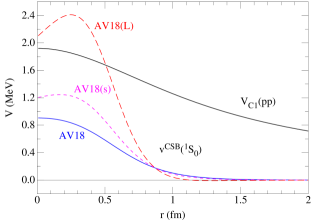
Figure 2: (Color online) Radial shapes of $v^{\rm CSB}$ in the ¹S₀ channel for the three different models AV18 (solid blue line), AV18(s) (short-dash magenta line), and AV18(L) (long-dash red line), compared to the proton-proton Coulomb interaction with form factor (solid black line).

III Quantum Monte Carlo method

We seek accurate solutions of the many-nucleon Schrödinger equation

$$H\Psi(J^{\pi};T,T_{z})=E\Psi(J^{\pi};T,T_{z})\ ,$$ (19)

where $\Psi(J^{\pi};T,T_{z})$ is a nuclear wave function with specific spin-parity $J^{\pi}$, isospin $T$, and charge state $T_{z}$. We begin with a variational Monte Carlo (VMC) calculation, constructing a variational function $\Psi_{V}(J^{\pi};T,T_{z})$ from products of two- and three-body correlation operators acting on an antisymmetric single-particle state of the appropriate quantum numbers. The correlation operators are designed to reflect the influence of the interactions at short distances, while appropriate boundary conditions are imposed at long range W91 ; PPCPW97 . The $\Psi_{V}(J^{\pi};T)$ has embedded variational parameters that are adjusted to minimize the expectation value

$$E_{V}=\frac{\langle\Psi_{V}|H|\Psi_{V}\rangle}{\langle\Psi_{V}|\Psi_{V}\rangle}\geq E_{0}\ ,$$ (20)

which is evaluated by Metropolis Monte Carlo integration MR2T2 . Here $E_{0}$ is the exact lowest eigenvalue of $H$ for the specified quantum numbers. A good variational trial function has the form

$$|\Psi_{V}\rangle={\cal S}\prod_{i<j}^{A}\left[1+U_{ij}+\sum_{k\neq i,j}^{A}\tilde{U}^{TNI}_{ijk}\right]|\Psi_{J}\rangle\ ,$$ (21)

where the ${\cal S}$ is a symmetrization operator. The Jastrow wave function $\Psi_{J}$ is fully antisymmetric and has the $(J^{\pi};T,T_{z})$ quantum numbers of the state of interest, while $U_{ij}$ and $\tilde{U}^{TNI}_{ijk}$ are the two- and three-body correlation operators. Although we construct the $\Psi_{V}(J^{\pi};T,T_{z})$ to be an eigenstate of the isospin $T$, we allow isobaric analog states with different $T_{z}$ to have different wave functions, reflecting primarily the difference in Coulomb contributions.

The GFMC method C87 ; C88 improves on the VMC wave functions by acting on $\Psi_{V}$ with the operator $\exp\left[-\left(H-E_{0}\right)\tau\right]$. In practice, a simplified version $H^{\prime}$ of the Hamiltonian $H$ is used in the operator, which includes the isoscalar part of the kinetic energy, a charge-independent eight-operator projection of AV18 called AV8^′, a strength-adjusted version of the three-nucleon potential IL7^′ (adjusted so that $\langle H^{\prime}\rangle\sim\langle H\rangle$), and an isoscalar Coulomb term that integrates to the total charge of the given nucleus KNBSK99 . The difference between $H$ and $H^{\prime}$ is calculated using perturbation theory. More detail can be found in Refs. PPCPW97 ; WPCP00 .

The operator is applied in small slices of imaginary time $\tau$ to produce a propagated wave function:

$$\Psi(\tau)=e^{-({H^{\prime}}-E_{0})\tau}\Psi_{V}=\left[e^{-({H^{\prime}}-E_{0})\triangle\tau}\right]^{n}\Psi_{V}\ .$$ (22)

Obviously $\Psi(\tau=0)=\Psi_{V}$ and $\Psi(\tau\rightarrow\infty)=\Psi_{0}$. The algorithm for propagation produces samples of the wave function $\Psi(\tau)$ but does not provide gradient information. Quantities of interest are evaluated in terms of a “mixed” expectation value between $\Psi_{V}$ and $\Psi(\tau)$:

$$\langle O(\tau)\rangle_{M} = \frac{\langle\Psi(\tau)|O|\Psi_{V}\rangle}{\langle\Psi(\tau)|\Psi_{V}\rangle},$$ (23)

where the operator $O$ acts on the trial function $\Psi_{V}$. The desired expectation values, of course, have $\Psi(\tau)$ on both sides; by writing $\Psi(\tau)=\Psi_{V}+\delta\Psi(\tau)$ and neglecting terms of order $[\delta\Psi(\tau)]^{2}$, we obtain the approximate expression

$$\langle O(\tau)\rangle = \frac{\langle\Psi(\tau)|O|\Psi(\tau)\rangle}{\langle\Psi(\tau)|\Psi(\tau)\rangle}$$ (24)

$$\approx \langle O(\tau)\rangle_{M}+[\langle O(\tau)\rangle_{M}-\langle O\rangle_{V}]~{},$$

where $\langle O\rangle_{\rm V}$ is the variational expectation value.

For off-diagonal matrix elements relevant to this work the generalized mixed estimate is given by the expression

$$\frac{\langle\Psi^{f}(\tau)|O|\Psi^{i}(\tau)\rangle}{\sqrt{\langle\Psi^{f}(\tau)|\Psi^{f}(\tau)\rangle}\sqrt{\langle\Psi^{i}(\tau)|\Psi^{i}(\tau)\rangle}}$$ (25)

$$\approx \langle O(\tau)\rangle_{M_{i}}+\langle O(\tau)\rangle_{M_{f}}-\langle O\rangle_{V}\ ,$$

where

$$\langle O(\tau)\rangle_{M_{f}} = \frac{\langle\Psi^{f}(\tau)|O|\Psi^{i}_{V}\rangle}{\langle\Psi^{f}(\tau)|\Psi^{f}_{V}\rangle}\sqrt{\frac{\langle\Psi^{f}_{V}|\Psi^{f}_{V}\rangle}{\langle\Psi^{i}_{V}|\Psi^{i}_{V}\rangle}}\ ,$$ (26)

and $\langle O(\tau)\rangle_{M_{i}}$ is defined similarly. For more details see Eqs. (19-24) and the accompanying discussions in Ref. PPW07 .

Table 3: Contributions to the isovector energy difference $E(^{3}{\rm He})-E(^{3}{\rm H})$ in keV from different interaction models; Monte Carlo statistical errors are shown in parentheses.

	AV18	AV18(s)	AV18(L)
$K^{\rm CSB}$	14(0)	14(0)	14(0)
$V_{C1}(pp)$	642(1)	642(1)	642(1)
$V_{C+}$	9(0)	9(0)	9(0)
$V_{MM}$	17(0)	17(0)	17(0)
$v^{\rm CSB}$	65(0)	71(0)	79(0)
$\delta H^{\rm CI}$	8(1)	8(1)	8(1)
$H^{\rm CSB}$	755(1)	761(1)	769(1)
Experiment			764

IV Results

IV.1 Energies of Ground and Excited States in ⁸Be

The GFMC energy for the ground state and the excitation energies for the first eight positive-parity excited states of ⁸Be are given in Table 1; these have been calculated for pure isospin states of either $T$=0 or $T$=1. The experimentally observed energies and the empirical energies for the unmixed states (derived as discussed in Sec. I) are also shown, along with the GFMC rms point proton radii. As discussed in Datar13 , the physically wide $2^{+}$ and $4^{+}$ states present a challenge for GFMC calculations because they tend to break up into separate $\alpha$ particles as the propagation in imaginary time $\tau$ proceeds. The energy drifts lower and the radii increase with $\tau$, so care is necessary to extract these quantities from the calculations. However, no such problem occurs for the physically much narrower $2^{+}$, $1^{+}$ and $3^{+}$ doublets; their GFMC energies and radii are quite stable as $\tau$ increases.

The AV18+IL7 Hamiltonian reproduces both the 2$\alpha$-like $0^{+}$, $2^{+}$, $4^{+}$ rotational band and the mixed $2^{+}$ and $1^{+}$ doublets exceptionally well Only the $3^{+}$ doublet is about 0.5 MeV too high in excitation energy, and with perhaps too big an energy difference between the states. The radii of the mixed doublets are all slightly smaller than the 2$\alpha$-like states. The energies and other properties of the isobaric analog states in ⁸Li and ⁸B are also in good agreement with experiment for this Hamiltonian PPSW13 .

IV.2 Isovector Energy Differences of Mirror Nuclei

We next examine the effect of our different interaction models on the isovector energy differences in $A$=3, $A$=7,$T$=$\frac{1}{2}$, and $A$=8,$T$=1 mirror nuclei. The energy difference $E(^{3}{\rm He})-E(^{3}{\rm H})$ for two correlated GFMC propagations BPW11 is given in Table 3. The starting variational wave functions were separately optimized for the two different charge states with the proper experimental charge radii. As stated above, the propagation is made with AV8^′+IL7^′ plus an isoscalar Coulomb term that integrates to the proper total charge for each nucleus, and the difference with AV18+IL7 or the variants of AV18 is evaluated using perturbation theory.

Table 4: Contributions to the isovector energy difference $E(^{7}{\rm Be})-E(^{7}{\rm Li})$ in keV from different interaction models; Monte Carlo statistical errors are shown in parentheses.

	AV18	AV18(s)	AV18(L)
$K^{\rm CSB}$	23(0)	23(0)	23(0)
$V_{C1}(pp)$	1442(2)	1442(2)	1442(2)
$V_{C+}$	18(0)	18(0)	18(0)
$V_{MM}$	18(0)	18(0)	18(0)
$v^{\rm CSB}$	83(1)	90(1)	105(1)
$\delta H^{\rm CI}$	27(10)	27(10)	27(10)
$H^{\rm CSB}$	1611(10)	1618(10)	1633(10)
Experiment			1645

The different contributions include 1) the kinetic energy $K^{\rm CSB}$, 2) the static Coulomb term between two protons (with finite-range form factor) $V_{C1}(pp)$, 3) all additional charge contributions to the electromagnetic interaction $V_{C+}$ (like Darwin-Foldy and vacuum polarization), 4) the magnetic moment term $V_{MM}$, and 5) the strong class III CSB term $v^{\rm CSB}$, which is the single term from AV18 or the sum of the first four rows of Eq.(II) for AV18(s) and AV18(L). The net change in the energy arising from the CI part of the Hamiltonian $\delta H^{\rm CI}$ is an additional second-order perturbation correction due to differences in the two GFMC propagations. This term is small for the $A$=3 case, although the changes in separate kinetic and potential parts are much larger.

(We note that the original $V_{C1}(pp)$ from Eq.(4) of Ref. WSS95 uses an $\alpha^{\prime}$ that has a small relativistic energy-dependence; we drop this from the many-body calculations and just use $\alpha$, which is what we mean by the term “static” Coulomb. However, we add a momentum-dependent orbit-orbit term to the $V_{C+}$, which is typically $\sim$1% of the static term, to approximate this term.)

The dominant contribution to the isovector energy difference is of course the static Coulomb interaction between protons, which is in agreement with model-independent estimates based on the experimental form factors BCS78 . Comparing the three different models for $v^{\rm CSB}$, the smallest is AV18, with AV18(s) being about 10% larger and AV18(L) about 20% larger, as might be expected from the larger size of $v^{CSB}$ in the ¹S₀ channel shown in Fig. 2. All the models give reasonable agreement with the experimental difference of 764 keV.

The isovector energy differences for the $A$=7,$T$=$\frac{1}{2}$ mirror nuclei are shown in Table 4. Again we show the difference of two correlated GFMC propagations BPW11 that have been started from separately optimized variational trial functions. The change in the CI part of the Hamiltonian $\delta H^{\rm CI}$ is larger than for $A$=3 and has a larger error bar, which now dominates the total error in $H^{\rm CSB}$. The net GFMC results are a little smaller than the experimental energy difference of 1645 keV. The $v^{\rm CSB}$ again increases about 20% going from AV18 to AV18(s) to AV18(L) as in the $A$=3 case, because the CSB force is being probed primarily in $S$=0, $T$=1 pairs embedded in the $p$-shell W06 .

Finally, the $A$=8,$T$=1 isovector energy difference $[E(^{8}{\rm B})-E(^{8}{\rm Li})]/2$ is shown in Table 5. The static Coulomb contribution is similar to the $A$=7 case, while the magnetic moment contribution almost vanishes. Notably, the variation between the AV18, AV18(s), and AV18(L) models is different, probably because there are now equal numbers of $S$=0 and 1, $T$=1 pairs embedded in the $p$-shell W06 and the spin-dependence of Eq.(II) comes into play. The change in the CI Hamiltonian $\delta H^{\rm CI}$ is similar to that in $A$=7 and the total $H^{\rm CSB}$ is somewhat over-predicted compared to the experimental value of 1770 keV.

Table 5: Contributions to the isovector energy difference $[E(^{8}{\rm B})-E(^{8}{\rm Li})]/2$ in keV from different interaction models; Monte Carlo statistical errors are shown in parentheses.

	AV18	AV18(s)	AV18(L)
$K^{\rm CSB}$	25(0)	25(0)	25(0)
$V_{C1}(pp)$	1652(3)	1652(3)	1652(3)
$V_{C+}$	17(0)	17(0)	17(0)
$V_{MM}$	1(0)	1(0)	1(0)
$v^{\rm CSB}$	77(1)	75(2)	84(3)
$\delta H^{\rm CI}$	33(11)	33(11)	33(11)
$H^{\rm CSB}$	1813(11)	1811(11)	1820(11)
Experiment			1770

In all three pairs of mirror nuclei, the static Coulomb interaction between protons is the dominant source of the energy difference, providing about 85-90% of the total, increasing as $A$ increases. The kinetic and remaining electromagnetic terms provide another few percent, leaving the remaining amount due to strong CSB terms. However, these terms are of shorter range than Coulomb, and their total contributions do not grow as rapidly with $A$, so they become relatively less important in larger nuclei.

IV.3 Isospin-Mixing Matrix Elements in ⁸Be

The GFMC evaluation for the IM matrix element $H_{01}$ between the $2^{+}$ states at 16.6–16.9 MeV excitation in ⁸Be is given in Table 6. The first five lines give the contributions for the same terms as in the energy differences for mirror nuclei of Tables 3–5. In addition there are rows for the additional class IV CSB terms: $v^{\rm IV}_{\gamma}$ of Eq.(13), $v^{\rm IV}_{\pi+\rho}$ of Eq.(II), and the antisymmetric spin-orbit term $v^{\rm IV}_{\rho\omega}$ that is the last line of Eq.(II).

We note that our Coulomb term of $-89$ keV is about 30% larger than Barker’s original estimate of $-67$ keV Barker66 . The additional electromagnetic and kinetic terms that we include give $-15$ keV, while the strong CSB terms add another $-24$ to $-28$ keV to the total. Thus, the strong CSB terms are relatively more important here than in the isovector energy differences between mirror nuclei, making this system one of the best for constraining such forces. The variation between AV18 and the alternative models AV18(s) and AV18(L) is proportionately the same as in the energy differences. Our total of $-127$ to $-131$ keV is about 90% of the empirical matrix element of $-145$ keV.

Table 6: Contributions to the isospin-mixing matrix element between ⁸Be($2^{+}$) states at 16.6–16.9 MeV excitation for different interaction models in keV; Monte Carlo statistical errors are shown in parentheses.

	AV18	AV18(s)	AV18(L)
$K^{\rm CSB}$	$-3.6(1)$	$-3.6(1)$	$-3.6(1)$
$V_{C1}(pp)$	$-89.3(11)$	$-89.3(11)$	$-89.3(11)$
$V_{C+}$	$0.0(0)$	$0.0(0)$	$0.0(0)$
$V_{MM}$	$-10.2(2)$	$-10.2(2)$	$-10.2(2)$
$v^{\rm CSB}$	$-23.4(4)$	$-24.7(6)$	$-25.7(10)$
$v^{\rm IV}_{\gamma}$	$-0.8(1)$	$-0.8(1)$	$-0.8(1)$
$v^{\rm IV}_{\pi+\rho}$		$-0.8(1)$	$-0.8(1)$
$v^{\rm IV}_{\rho\omega}$		$-0.3(1)$	$-0.8(3)$
$H_{01}$	$-127.(2)$	$-130.(2)$	$-131.(2)$
Experiment			$-145.(3)$

Table 7: Contributions to the isospin-mixing matrix element between ⁸Be($1^{+}$) states at 17.6–18.1 MeV excitation for different interaction models in keV; Monte Carlo statistical errors are shown in parentheses.

	AV18	AV18(s)	AV18(L)
$K^{\rm CSB}$	$-2.8(1)$	$-2.8(1)$	$-2.8(1)$
$V_{C1}(pp)$	$-73.4(11)$	$-73.4(11)$	$-73.4(11)$
$V_{C+}$	$0.0(0)$	$0.0(0)$	$0.0(0)$
$V_{MM}$	$-1.1(1)$	$-1.1(1)$	$-1.1(1)$
$v^{\rm CSB}$	$-18.5(4)$	$-18.7(6)$	$-19.9(10)$
$v^{\rm IV}_{\gamma}$	$2.1(1)$	$2.1(1)$	$2.1(1)$
$v^{\rm IV}_{\pi+\rho}$		$0.2(0)$	$0.2(0)$
$v^{\rm IV}_{\rho\omega}$		$0.5(1)$	$1.1(2)$
$H_{01}$	$-94.(1)$	$-93.(2)$	$-94.(2)$
Experiment			$-103.(14)$

The GFMC evaluation for the IM matrix element $H_{01}$ between the $1^{+}$ states at 17.6–18.2 MeV excitation in ⁸Be is given in Table 7. In this case, our $pp$ Coulomb term of $-73$ keV is 35% larger than Barker’s estimate of $-54$ keV. The strong class III CSB term is a little bit smaller than in the $2^{+}$ case. The magnetic moment term almost vanishes, and the class IV CSB terms reduce the magnitude of the mixing matrix element. This change of sign of the ${\bf L}\cdot{\bf A}$ terms relative to the $2^{+}$ (and $3^{+}$) doublets is probably due to the significant admixture of ¹P₁[431] symmetry components in the $T$=1 state. In the end, the three interaction models again give a very narrow spread of $-93$ to $-94$ keV, or about 90% of the empirical value of $-103$ keV.

The GFMC evaluation for the IM matrix element $H_{01}$ between the $3^{+}$ states at 19.0–19.2 MeV excitation in ⁸Be is given in Table 8. The Coulomb term at $-75$ keV is comparable to the previous cases, but now more than double Barker’s estimate of $-32$ keV. The strong class III CSB terms are similar to the previous cases. The regular magnetic moment contribution is like that in the $2^{+}$ doublet, but the class IV magnetic moment term is larger. Overall, there is again very little spread between our models, at $-111$ to $-115$ keV, but these are now much larger than the poorly determined value of $-59$ keV for the empirical matrix element. Further, the maximum possible IM matrix element is one half the spacing between the two physical states, which in this case is 165(32) keV. The experimental energy difference would have to be about two standard deviations greater than given in the compilation exp8-10 to admit an IM matrix element as large as that predicted by our Hamiltonian. The GFMC calculations do hint at a bigger energy difference between the isospin-pure states as shown in Table 1.

Table 8: Contributions to the isospin-mixing matrix element between ⁸Be($3^{+}$) states at 19.0–19.2 MeV excitation for different interaction models in keV; Monte Carlo statistical errors are shown in parentheses.

	AV18	AV18(s)	AV18(L)
$K^{\rm CSB}$	$-3.0(1)$	$-3.0(1)$	$-3.0(1)$
$V_{C1}(pp)$	$-74.6(12)$	$-74.6(12)$	$-74.6(12)$
$V_{C+}$	$0.0(0)$	$0.0(0)$	$0.0(0)$
$V_{MM}$	$-12.3(2)$	$-12.3(2)$	$-12.3(2)$
$v^{\rm CSB}$	$-16.6(4)$	$-16.9(6)$	$-17.5(10)$
$v^{\rm IV}_{\gamma}$	$-4.5(1)$	$-4.5(1)$	$-4.5(1)$
$v^{\rm IV}_{\pi+\rho}$		$-0.3(0)$	$-0.3(0)$
$v^{\rm IV}_{\rho\omega}$		$-1.3(1)$	$-2.5(0)$
$H_{01}$	$-111.(2)$	$-112.(2)$	$-115.(2)$
Experiment			$-59.(12)$

Finally we report the IM matrix element between the first $2^{+}$ $T$=0 state in ⁸Be at 3.0 MeV excitation and the $2^{+}$ $T$=1 state at 16.8 MeV. The former is the final state for $\beta$-decay from both ⁸Li and ⁸B ground states, while the latter is the isobaric analog of the initial states. These transitions have been used to search for tensor components in nuclear $\beta$-decay bdecay13 and may be used in future experiments to search for second-class currents or other violations of the conserved vector-current hypothesis. The analysis of such experiments relies on the final state being a $T$=0 state with a negligible $T$=1 component. Without giving the detailed breakdown, we get an IM matrix element of $-7(2)$ keV which, combined with the large separation in energy, implies an amplitude admixture of the first $2^{+}$ $T$=1 state into the first $2^{+}$ $T$=0 state of $5.0(1.5)\times 10^{-4}$. This is sufficiently small to not interfere with the goal stated in Ref. bdecay13 of improving the limit on tensor components by an order of magnitude.

V Conclusions

In summary, we have reported GFMC results for IM matrix elements in the $2^{+}$, $1^{+}$, and $3^{+}$ doublets at 16–19 MeV excitation in the spectrum of ⁸Be. We have made these calculations for the AV18+IL7 Hamiltonian and two variants of AV18 with an expanded CSB operator structure, all constrained to give the same $nn$ scattering length. The AV18+IL7 model gives an excellent reproduction of the ⁸Be spectrum and a good description of the energy differences in $A$=3, 7 and 8 mirror nuclei. For the isospin-mixing matrix element, we add the class IV CSB terms that come from one-photon, one-pion, one-rho, and rho-omega mixing. We have not considered possible three-nucleon CSB forces, which have been estimated to contribute $\sim 5$ keV to the ³He–³H energy difference FPvK05 . We obtain about 90% of the empirical IM matrix elements for the $2^{+}$ and $1^{+}$ doublets, but we overpredict the less well-measured $3^{+}$ doublet. New experiments for these latter states would be useful.

Our main conclusion is that, while the static Coulomb interaction between protons is the dominant contributor to CSB in nuclei, the additional electromagnetic, kinetic, and strong CSB terms are important, and the IM matrix elements in ⁸Be are a particularly valuable place to look for their effect.

- (1) D. R. Tilley, J. H. Kelley, J. L. Godwin, D. J. Millener, J. Purcell, C. G. Sheu, and H. R. Weller, Nucl. Phys. A745, 155 (2004).
- (2) R. B. Wiringa, Phys. Rev. C 73, 034317 (2006).
- (3) R. B. Wiringa, S. C. Pieper, J. Carlson, and V. R. Pandharipande, Phys. Rev. C 62, 014001 (2000).
- (4) F. C. Barker, Nucl. Phys. 83, 418 (1966).
- (5) M. A. Oothoudt and G. T. Garvey, Nucl. Phys. A284, 41 (1977).
- (6) E. M. Henley and G. A. Miller, in Mesons in Nuclei, edited by M. Rho and D. H. Wilkinson (North-Holland, Amsterdam, 1979), p. 405; G. A. Miller, B. M. K. Nefkens and I. Slaus, Phys. Rept. 194, 1 (1990).
- (7) U. van Kolck, J. L. Friar, and T. Goldman, Phys. Lett. B 371, 169 (1996).
- (8) R. B. Wiringa, V. G. J. Stoks, and R. Schiavilla, Phys. Rev. C 51, 38 (1995).
- (9) S. C. Pieper, V. R. Pandharipande, R. B. Wiringa, and J. Carlson, Phys. Rev. C 64, 014001 (2001).
- (10) S. C. Pieper, AIP Conf. Proc. 1011, 143 (2008).
- (11) G. F. de Téramond and B. Gabioud, Phys. Rev. C 36, 691 (1987).
- (12) R. Machleidt and I. Slaus, J. Phys. G 27, R69 (2001).
- (13) J. L. Friar and B. F. Gibson, Phys. Rev. C 17, 1752 (1978).
- (14) P. C. McNamee, M. D. Scadron, and S. A. Coon, Nucl. Phys. A249, 483 (1975); S. A. Coon, M. D. Scadron, and P. C. McNamee, Nucl. Phys. A287, 381 (1997).
- (15) A. G. Williams, A. W. Thomas, and G. A. Miller, Phys. Rev. C 36, 1956 (1987); G. A. Miller, A. W. Thomas and A. G. Williams, Phys. Rev. Lett. 56, 2567 (1986).
- (16) R. Abegg, et al., Phys. Rev. Lett. 56, 2571 (1986); R. Abegg, et al., Phys. Rev. D 39, 2464 (1989); R. Abegg, et al., Phys. Rev. Lett. 75, 1711 (1995); J. Zhao, et al., Phys. Rev. C 57, 2126 (1998).
- (17) L. D. Knutson, S. E. Vigdor, W. W. Jacobs, J. Sowinski, P. L. Jolivette, S. W. Wissink, C. Bloch, C. Whiddon, and R. C. Byrd, Phys. Rev. Lett. 66, 1410 (1991); S. E. Vigdor, W. W. Jacobs, L. D. Knutson, J. Sowinski, C. Bloch, P. L. Jolivette, S. W. Wissink, R. C. Byrd, and C. Whiddon, Phys. Rev. C 46, 410 (1992).
- (18) R. B. Wiringa, Phys. Rev. C 43, 1585 (1991).
- (19) B. S. Pudliner, V. R. Pandharipande, J. Carlson, S. C. Pieper, and R. B. Wiringa, Phys. Rev. C 56, 1720 (1997).
- (20) N. Metropolis, A. W. Rosenbluth, M. N. Rosenbluth, A. H. Teller, and E. Teller, J. Chem. Phys. 21, 1087 (1953).
- (21) J. Carlson, Phys. Rev. C 36, 2026 (1987).
- (22) J. Carlson, Phys. Rev. C 38, 1879 (1988).
- (23) G. P. Kamuntavičius, P. Navrátil, B. R. Barrett, G. Sapragonaite, and R. K. Kalinauskas, Phys. Rev. C 60, 044304 (1999).
- (24) M. Pervin, S. C. Pieper, and R. B. Wiringa, Phys. Rev. C 76, 064319 (2007).
- (25) I. Brida, S. C. Pieper, and R. B. Wiringa, Phys. Rev. C 84, 024319 (2011).
- (26) R. A. Brandenburg, S. A. Coon, and P. U. Sauer, Nucl. Phys. A 294, 305 (1978).
- (27) V. M. Datar, et al., Phys. Rev. Lett. 111, 062502 (2013).
- (28) S. Pastore, S. C. Pieper, R. Schiavilla, and R. B. Wiringa, Phys. Rev. C 87, 035503 (2013).
- (29) G. Li, et al., Phys. Rev. Lett. 110, 092502 (2013).
- (30) J. L. Friar, G. L. Payne, and U. van Kolck, Phys. Rev. C 71, 024003 (2005).