Following a Trend with an Exponential Moving Average: Analytical Results for a Gaussian Model

Abstract

We investigate how price variations of a stock are transformed into profits and losses (P&Ls) of a trend following strategy. In the frame of a Gaussian model, we derive the probability distribution of P&Ls and analyze its moments (mean, variance, skewness and kurtosis) and asymptotic behavior (quantiles). We show that the asymmetry of the distribution (with often small losses and less frequent but significant profits) is reminiscent to trend following strategies and less dependent on peculiarities of price variations. At short times, trend following strategies admit larger losses than one may anticipate from standard Gaussian estimates, while smaller losses are ensured at longer times. Simple explicit formulas characterizing the distribution of P&Ls illustrate the basic mechanisms of momentum trading, while general matrix representations can be applied to arbitrary Gaussian models. We also compute explicitly annualized risk adjusted P&L and strategy turnover to account for transaction costs. We deduce the trend following optimal timescale and its dependence on both auto-correlation level and transaction costs. Theoretical results are illustrated on the Dow Jones index.

1 Introduction

Systematic trading has grown as an industry in finance, allowing to take rapid trading decisions for multiple stocks [1, 2, 3, 5, 4, 6, 7]. A strategy relies on price time series in the past in order to forecast price variations in near future and update accordingly its positions. Although the market complexity, variability and stochasticity damn such forecasting to fail in nearly half cases, even a tiny excess of successful forecasts is enhanced by a very large number of trades into statistically relevant profits. Many trading strategies attempt to detect an eventual trend in price series, i.e., a sequence of positively auto-correlated price variations which may be caused, e.g., by a news release or common activity of multiple traders. From a practical point of view, a strategy transforms the known past information into a signal for buying or selling a number of shares. From a mathematical point of view, systematic trading can be seen as a transformation of price time series into profit-and-loss (P&L) time series of the strategy, as illustrated on Fig. 1. For instance, the passive (long) strategy of buying and holding a stock corresponds to the identity transformation. The choice for the optimal strategy depends on the imposed risk-reward criteria.

In this paper, we study the transformation of price variations into P&Ls of a trend following strategy based on an exponential moving average (EMA). This archetypical strategy turns out to be the basis for many systematic trading platforms [1, 2, 3, 5, 4, 6, 7], while other methods such as the detrending moving average analysis or higher-order moving averages can also be employed [8, 9, 10, 11]. A trend following strategy is known to skew the probability distribution of P&Ls [12, 13], as we illustrate on Fig. 2. This figure shows how empirically computed quantiles of price variations are transformed into quantiles of P&Ls for the Dow Jones index (1900-2012). Even for such a long sample with 30733 daily returns, accurate estimation of quantiles remains problematic. Moreover, the basic mechanisms of this transformation remain poorly understood. For these reasons, we will study a simple model in which standardized logarithmic returns are Gaussian random variables [14] whose auto-correlations reflect random trends. Even though heavy tailed asymptotic distribution of returns and some other stylized facts are ignored [15, 16, 17, 18, 19, 20, 21, 22, 23, 24], the Gaussian hypothesis will allow us to derive analytical results that can be later confronted to empirical market data. We will compute the probability distribution of P&Ls of a trend following strategy in order to understand how the Gaussian distribution of price variations is transformed by systematic trading. The respective roles of the market (positive auto-correlations) and of the strategy itself, onto profits and losses, will therefore be disentangled.

The paper is organized as follows. In Sec. 2, we introduce matrix notations, a market model and a trend following strategy. Main results about the probability distribution and moments of P&Ls are presented in Sec. 3. Discussion, conclusion and perspectives are summarized in Sec. 4.

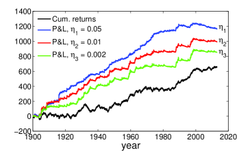
Figure 1: Cumulative standardized logarithmic returns (normalized by realized volatility) of the Dow Jones index, from 1900 to 2012 (black curve), and cumulative P&Ls of trend following strategies (defined in Sec. 2) with timescales $\eta_{1}=0.05$ (blue), $\eta_{2}=0.01$ (red), and $\eta_{3}=0.002$ (green), applied to this index.

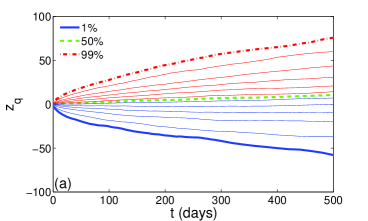
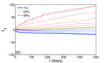
Figure 2: Comparison between quantiles of buy-and-hold strategy and trend following strategy. (a) Quantiles of cumulative standardized logarithmic returns (normalized by realized volatility) of the Dow Jones index (1900-2012) as functions of lag time $t$ (in days). Lines from the bottom to the top show quantiles with $1\%$, $5\%$, $15\%$, $25\%$, $35\%$, $45\%$ (blue color), $50\%$ (green color), $55\%$, $65\%$, $75\%$, $85\%$, $95\%$, and $99\%$ (red color), respectively. Thick lines highlight $1\%$, $50\%$ and $99\%$ quantiles. (b) Quantiles of cumulative P&Ls of a trend following strategy with the timescale $\eta=0.01$, applied to the Dow Jones index (same notations).

2 Market model and trading strategy

2.1 Exponential moving average

The exponential moving average (EMA) is broadly employed in signal processing and data analysis [25, 26, 27, 28]. The EMA can be defined as a linear transformation of a time series $\{x_{t}\}$ to a smoother time series $\{\tilde{x}_{t}\}$ according to

$$\tilde{x}_{t}=\lambda\sum\limits_{k=0}^{\infty}(1-\lambda)^{k}x_{t-k},$$ (1)

where $0<\lambda\leq 1$ is the (inverse of) timescale. When $\lambda=1$, the EMA is the identity transformation: $\tilde{x}_{t}=x_{t}$; in contrast, many terms $x_{t-k}$ effectively contribute to $\tilde{x}_{t}$ when $\lambda\ll 1$. The EMA is often preferred to simple moving average over a window of fixed length because it yields smoother results. In practice, it can be computed in real time according to a recurrent formula:

$$\tilde{x}_{t}=(1-\lambda)\tilde{x}_{t-1}+\lambda x_{t}.$$

When a time series starts from $t=1$, the non-existing elements $x_{0}$, $x_{-1}$, $x_{-2}$, … are set to $0$. This is equivalent to setting the upper limit in Eq. (1) to $t-1$. In the analysis of a finite sample of length $T$, the EMA can be written in a matrix form as

$$\left(\begin{array}[]{c}\tilde{x}_{1}\\ ...\\ \tilde{x}_{T}\\ \end{array}\right)=\lambda{\bf E}_{1-\lambda}\left(\begin{array}[]{c}x_{1}\\ ...\\ x_{T}\\ \end{array}\right),$$

where ${\bf E}_{q}$ is the matrix of size $T\times T$, whose elements are

$$({\bf E}_{q})_{jk}=\begin{cases}q^{j-k-1}\quad(j>k),\cr 0\hskip 36.98857pt(j\leq k).\end{cases}$$ (2)

2.2 Gaussian market models

The first Gaussian market model was introduced by Bachelier in 1900 and since that time, numerous models have been developed. For instance, the class of ARMA (Auto-Regressive Moving Average) models and their extensions were thoroughly employed in finance [25]. During decades, these models were getting more and more elaborate in order to account for various empirical features of markets. Our purpose is the opposite: we aim at understanding the basic mechanisms of trend following strategies, and we expect that qualitatively, these mechanisms weakly depend on market peculiarities. In turn, the quantitative behavior of P&Ls may of course be sensitive to particular features. For this reason, we choose a simple model exhibiting random trends, in order to be able to derive analytical results. At the same time, general matrix formulas used in this paper (see the beginning of Sec. 3) can be applied to arbitrary Gaussian market model. In this light, our methodology can be used for studying more elaborate models, though results will be less explicit.

In this paper, we consider a simple model of daily price variations, or returns, $r_{t}$, in which random trends are induced by a discrete Ornstein-Uhlenbeck process, while short-time fluctuations are modeled by iid Gaussian variables $\varepsilon_{k}\in{\mathcal{N}}(0,1)$ with zero mean and unit variance:

$$r_{t}=\varepsilon_{t}+\beta\sum\limits_{k=1}^{t-1}(1-\lambda)^{t-1-k}\xi_{k},$$ (3)

where $\lambda$ and $\beta$ are two parameters of the market model describing the characteristic timescale and the strength of the trend contribution, and $\xi_{k}\in{\mathcal{N}}(0,1)$ are iid Gaussian variables (independent of $\varepsilon_{k}$). This is a model of stochastic trends which are induced by a persistent process generated by exogeneous random variables $\xi_{k}$ which are independent from the short-time fluctuations $\varepsilon_{k}$. In a matrix form, one writes

$${\bf r}=\varepsilon+\beta{\bf E}_{1-\lambda}\xi,$$ (4)

where ${\bf r}=(r_{1},...,r_{T})^{\dagger}$ is the vector of returns (the superscript ${\dagger}$ denoting the transpose), and $\varepsilon$ and $\xi$ are two vectors of iid Gaussian variables. As a consequence, ${\bf r}$ is a Gaussian vector with zero mean, $\langle r_{j}\rangle=0$, and the covariance matrix ${\bf C}_{j,k}=\langle r_{j}r_{k}\rangle$, for which

$${\bf C}={\bf I}+\beta^{2}{\bf E}_{1-\lambda}{\bf E}_{1-\lambda}^{\dagger},$$ (5)

where ${\bf I}$ stands for the identity matrix. The elements of this matrix are

$${\bf C}_{j,k}=\delta_{j,k}+\frac{\beta^{2}}{\lambda(2-\lambda)}\biggl{[}(1-\lambda)^{|j-k|}-(1-\lambda)^{j+k-2}\biggr{]}.$$ (6)

The second term is the covariance of a discrete Ornstein-Uhlenbeck process. The diagonal elements ${\bf C}_{t,t}$ approach the constant $\sigma_{\infty}^{2}=1+\frac{\beta^{2}}{\lambda(2-\lambda)}$ as $t\to\infty$, i.e., auto-correlations increase the variance of returns. It is convenient to make the limiting variance $\sigma_{\infty}^{2}$ independent of the timescale $\lambda$ by rescaling the parameter $\beta$ as

$$\beta=\beta_{0}\sqrt{\lambda(2-\lambda)},$$ (7)

so that $\sigma_{\infty}^{2}=1+\beta_{0}^{2}$, independently of $\lambda$. In other words, the new parameter $\beta_{0}^{2}$ is the asymptotic excess variance of returns due to their auto-correlations. This parameter can be calibrated from empirical price series. For this purpose, we consider the variogram of returns over the lag time $t$

$$V_{t,t_{0}}\equiv\frac{{\rm var}\{r_{t_{0}+1}+...+r_{t_{0}+t}\}}{{\rm var}\{r_{t_{0}+1}\}+...+{\rm var}\{r_{t_{0}+t}\}},$$ (8)

where an initiation period of duration $t_{0}$ can be ignored to approach the stationary regime. The variogram would be equal to $1$ for iid random variables, while its deviations from $1$ characterize auto-correlations between variables. Expressing the variogram through the covariance matrix in Eq. (5), one gets in the stationary limit $t_{0}\to\infty$:

$$\lim\limits_{t_{0}\to\infty}{\rm var}\{r_{t_{0}+1}+...+r_{t_{0}+t}\}=t\biggl{[}1+\beta_{0}^{2}\frac{2-\lambda}{\lambda}\biggr{]}-\frac{2(1-\lambda)\beta_{0}^{2}}{\lambda^{2}}\bigl{(}1-(1-\lambda)^{t}\bigr{)}$$

and

$$V_{t,\infty}=1+\frac{2(1-\lambda)\beta_{0}^{2}}{\lambda(1+\beta_{0}^{2})}\biggl{(}1-\frac{1-(1-\lambda)^{t}}{\lambda t}\biggr{)}.$$ (9)

Figure 3 shows the empirical variogram of returns obtained from the Dow Jones index (1900-2012), and its fit according to Eq. (9). Although the model fails to reproduce a steep growth of auto-corrections at short times, it captures correctly the behavior of the variogram at longer times and allows us to get realistic values for the parameters $\lambda$ and $\beta_{0}$ of the model: $\lambda=0.011$ and $\beta_{0}=0.08$. At the same time, these values are market dependent and, in general, difficult to calibrate. In what follows, the representative values $\lambda=0.01$ and $\beta_{0}=0.1$ will be used for illustrative purposes.

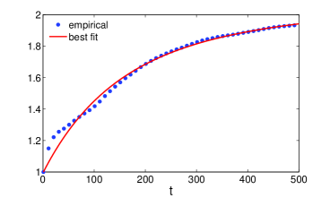
Figure 3: Variogram of standardized logarithmic daily returns (normalized by realized volatility) of the Dow Jones index (full circles) and its best fit to Eq. (9) (red line) with $\lambda=0.011$ and $\beta_{0}=0.08$.

For comparison, we also consider an auto-regressive model with exponential weights,

$$r_{t}=\varepsilon_{t}+\beta\sum\limits_{k=1}^{t-1}(1-\lambda)^{t-1-k}r_{k},$$ (10)

where $\varepsilon_{t}\in{\mathcal{N}}(0,1)$ are iid Gaussian variables. This is a model of autoregressive trends which are induced through auto-correlations with earlier returns. Writing Eq. (10) in a matrix form, ${\bf r}=\varepsilon+\beta{\bf E}_{1-\lambda}{\bf r}$ and inverting this relation yields

$${\bf r}=({\bf I}-\beta{\bf E}_{1-\lambda})^{-1}\varepsilon=({\bf I}+\beta{\bf E}_{1-\lambda+\beta})\varepsilon,$$ (11)

where the explicit matrix inversion was possible due to the specific triangular structure of the matrix ${\bf E}_{q}$. As a consequence, ${\bf r}$ is a Gaussian vector with zero mean and the covariance matrix

$${\bf C}=({\bf I}+\beta{\bf E}_{\tilde{q}})({\bf I}+\beta{\bf E}_{\tilde{q}})^{\dagger}={\bf I}+\beta({\bf E}_{\tilde{q}}+{\bf E}_{\tilde{q}}^{\dagger})+\beta^{2}{\bf E}_{\tilde{q}}{\bf E}_{\tilde{q}}^{\dagger},$$ (12)

where $\tilde{q}=1-\lambda+\beta$. Comparing this relation to Eq. (5), one notes the effective timescale $\lambda-\beta$ (instead of $\lambda$), and an additional term $\beta({\bf E}_{\tilde{q}}+{\bf E}_{\tilde{q}}^{\dagger})$. Although both models exhibit many similar features, they are not identical due to the presence of this term. For the sake of simplicity, we focus on the stochastic trend model (defined by Eq. (3)), while similar results for the auto-regressive trend model are derived and discussed in [30]. Qualitative conclusions of the paper do not depend on this choice.

It is worth noting that we focus on trends that are induced by auto-correlations, while mean returns are zero. While an extension to the case $\langle r_{t}\rangle\neq 0$ is relatively straightforward, the studied situation with $\langle r_{t}\rangle=0$ allows us to easier illustrate the role of trend following strategy because the passive holding strategy is profitless in this case.

2.3 Trading strategy

The trading strategy relies on an EMA of returns in order to detect eventual trends in price time series [25, 26, 27, 28]. We consider the signal $s_{t}$, which is proportional to the EMA of returns:

$$s_{t}=\gamma\sum\limits_{k=1}^{t-1}(1-\eta)^{t-1-k}r_{k},$$ (13)

where $\eta$ and $\gamma$ are two parameters of the strategy (in what follows, we will relate $\gamma$ to $\eta$, the latter remaining the only parameter of the strategy). It is crucial that the signal at time $t$ is determined by earlier returns $r_{t-1}$, $r_{t-2}$, … and does not rely on unavailable information on the present return $r_{t}$. In a matrix form, Eq. (13) reads as

$${\bf s}=\gamma{\bf E}_{1-\eta}{\bf r}.$$ (14)

The cumulative P&L of a trend following strategy after $t$ steps is defined as

$${\mathcal{P}}_{t,t_{0}}\equiv\sum\limits_{k=t_{0}+1}^{t+t_{0}}r_{k}s_{k}=({\bf r}^{\dagger}{\bf O}^{(t,t_{0})}{\bf s})=\gamma({\bf r}^{\dagger}{\bf O}^{(t,t_{0})}{\bf E}_{1-\eta}{\bf r})=\frac{1}{2}({\bf r}^{\dagger}{\bf M}^{(t,t_{0})}_{1-\eta}{\bf r}),$$ (15)

where $t_{0}$ is the duration of an initiation period,

$${\bf M}_{1-\eta}^{(t,t_{0})}\equiv\gamma\bigl{[}{\bf O}^{(t,t_{0})}{\bf E}_{1-\eta}+{\bf E}_{1-\eta}^{\dagger}{\bf O}^{(t,t_{0})}\bigr{]}$$ (16)

is a symmetric matrix, and ${\bf O}^{(t,t_{0})}$ is the matrix which has $1$ in the diagonal positions between $t_{0}+1$ and $t_{0}+t$, and $0$ elsewhere. The cumulative P&L in Eq. (15) is written as a quadratic form of the Gaussian vector ${\bf r}$. Similarly, an incremental P&L reads as

$$\delta{\mathcal{P}}_{\bar{t}}\equiv\delta{\mathcal{P}}_{t,t_{0}}\equiv{\mathcal{P}}_{t,t_{0}}-{\mathcal{P}}_{t-1,t_{0}}=r_{t+t_{0}}s_{t+t_{0}}=\frac{1}{2}({\bf r}^{\dagger}{\bf M}_{1-\eta}^{(1,{\bar{t}}-1)}{\bf r}),$$ (17)

where ${\bar{t}}=t+t_{0}$ is a shortcut notation for $t+t_{0}$.

3 Profit-and-loss of trend following strategy

The representations (15, 17) of cumulative and incremental P&Ls as quadratic forms of Gaussian vectors allow one to investigate their properties. For a discrete Gaussian process ${\bf r}$ with mean zero and covariance matrix ${\bf C}$, the quadratic form $\chi=\frac{1}{2}({\bf r}^{\dagger}{\bf M}{\bf r})$ defined by a symmetric matrix ${\bf M}$ is a random variable whose moments and probability distribution are well known [29]. In fact, a matrix representation of the characteristic function of $\chi$,

$$\phi(k)\equiv\langle\exp(ik\chi)\rangle=\frac{1}{\sqrt{\det({\bf I}-ik{\bf M}{\bf C})}},$$ (18)

yields the probability density $p(z)$ of $\chi$ through the inverse Fourier transform:

$$p(z)=\int\limits_{-\infty}^{\infty}\frac{dk}{2\pi}e^{-ikz}\phi(k).$$ (19)

As described in [29], the determinant $\det({\bf I}-ik{\bf M}{\bf C})$ can be expressed through the eigenvalues of the matrix ${\bf M}{\bf C}$ that speeds up numerical computations. Moreover, the smallest and the largest eigenvalues, $\mu_{-}$ and $\mu_{+}$, essentially determine the asymptotic behavior of the probability density $p(z)$:

$$p(z)\propto A_{\pm}z^{\nu_{\pm}}\exp(-z/\mu_{\pm})\quad(z\to\pm\infty)$$ (20)

(note that $\mu_{-}<0$ to ensure the decay of the density as $z\to-\infty$).

Finally, the cumulant moments $\kappa_{m}$ of the quadratic form $\chi$ are

$$\kappa_{m}=\frac{(m-1)!}{2}~{}{\rm tr}(({\bf M}{\bf C})^{m}),$$ (21)

where ${\rm tr}$ denotes the trace. In particular, $\kappa_{1}$ and $\kappa_{2}$ are the mean and variance of $\chi$, while higher-order cumulant moments determine the skewness ($\kappa_{3}/\kappa_{2}^{3/2}$) and kurtosis ($\kappa_{4}/\kappa_{2}^{2}$).

3.1 Mean incremental P&L

We first consider the incremental P&L, $\delta{\mathcal{P}}_{\bar{t}}$, for which the matrix ${\bf M}_{1-\eta}^{(1,{\bar{t}}-1)}$ from Eq. (16) has a particularly simple structure, with nonzero contributions only at ${\bar{t}}$-th row and column. The product of this matrix with the covariance matrix ${\bf C}$ can be written explicitly, e.g.,

$$\kappa_{1}=\frac{1}{2}{\rm tr}({\bf M}{\bf C})=\gamma\sum\limits_{k=1}^{{\bar{t}}-1}p^{{\bar{t}}-k-1}{\bf C}_{{\bar{t}},k},$$ (22)

where $p=1-\eta$. Substituting Eq. (5) into Eq. (22) yields the mean incremental P&L

$$\langle\delta{\mathcal{P}}_{\bar{t}}\rangle=\gamma\beta_{0}^{2}\biggl{[}q\frac{1-(pq)^{{\bar{t}}-1}}{1-pq}-q^{{\bar{t}}-1}\frac{p^{{\bar{t}}-1}-q^{{\bar{t}}-1}}{p-q}\biggr{]},$$ (23)

where $q=1-\lambda$. In the special case $\eta=\lambda$, this expression reduces to

$$\langle\delta{\mathcal{P}}_{\bar{t}}\rangle=\gamma\beta_{0}^{2}\biggl{[}q\frac{1-q^{2({\bar{t}}-1)}}{1-q^{2}}-({\bar{t}}-1)q^{2{\bar{t}}-3}\biggr{]}.$$ (24)

In the stationary limit $t_{0}\to\infty$ (we recall that ${\bar{t}}=t+t_{0}$), Eq. (23) yields the mean stationary daily P&L:

$$\langle\delta{\mathcal{P}}_{\infty}\rangle=\gamma\beta_{0}^{2}\frac{1-\lambda}{1-(1-\eta)(1-\lambda)}.$$ (25)

The mean cumulative P&L, $\langle{\mathcal{P}}_{t,t_{0}}\rangle$, can be obtained by summing contributions in Eq. (23). In the stationary limit $t_{0}\to\infty$, the mean cumulative P&L is simply proportional to $t$:

$$\langle{\mathcal{P}}_{t,\infty}\rangle=t~{}\langle\delta{\mathcal{P}}_{\infty}\rangle.$$

3.2 Variance of incremental P&L

The variance $v_{\bar{t}}$ of the incremental P&L, $\delta{\mathcal{P}}_{\bar{t}}$, is

$$v_{\bar{t}}\equiv\langle r_{\bar{t}}^{2}s_{\bar{t}}^{2}\rangle-\langle r_{\bar{t}}s_{\bar{t}}\rangle^{2}=\gamma^{2}\sum\limits_{j,k=1}^{{\bar{t}}-1}[{\bf E}_{1-\eta}]_{{\bar{t}},j}[{\bf E}_{1-\eta}]_{{\bar{t}},k}\bigl{[}\langle r_{\bar{t}}^{2}r_{j}r_{k}\rangle-\langle r_{\bar{t}}r_{j}\rangle\langle r_{\bar{t}}r_{k}\rangle\bigr{]}.$$

Since ${\bf r}$ is a Gaussian vector, the Wick’s theorem allows one to express the fourth-order correlation of Gaussian variables through the covariance matrix:

$$\langle r_{\bar{t}}^{2}r_{j}r_{k}\rangle=\langle r_{\bar{t}}^{2}\rangle~{}\langle r_{j}r_{k}\rangle+2\langle r_{\bar{t}}r_{j}\rangle\langle r_{\bar{t}}r_{k}\rangle={\bf C}_{{\bar{t}},{\bar{t}}}{\bf C}_{j,k}+2{\bf C}_{{\bar{t}},j}{\bf C}_{{\bar{t}},k},$$

from which

$$v_{\bar{t}}=\gamma^{2}\biggl{[}{\bf C}_{{\bar{t}},{\bar{t}}}({\bf E}_{1-\eta}{\bf C}{\bf E}_{1-\eta}^{\dagger})_{{\bar{t}},{\bar{t}}}+[({\bf E}_{1-\eta}{\bf C})_{{\bar{t}},{\bar{t}}}]^{2}\biggr{]}.$$ (26)

Substituting Eq. (5) yields

$$\begin{split}&v_{\bar{t}}=\gamma^{2}\biggl{\{}\bigl{(}1+\beta_{0}^{2}(1-q^{2{\bar{t}}-2})\bigr{)}\biggl{(}\frac{1-p^{2{\bar{t}}-2}}{1-p^{2}}+\frac{\beta_{0}^{2}(1-q^{2})}{(1-pq)(p-q)}\biggl{[}\frac{p(1-p^{2{\bar{t}}-2})}{1-p^{2}}-\\ &\frac{q(1-q^{2{\bar{t}}-2})}{1-q^{2}}-\frac{(p^{{\bar{t}}-1}-q^{{\bar{t}}-1})^{2}}{p-q}\biggr{]}\biggr{)}+\frac{\beta_{0}^{4}(1-q^{2})^{2}}{(p-q)^{2}}\biggl{[}\frac{1-(pq)^{{\bar{t}}-1}}{1-pq}-\frac{1-q^{2{\bar{t}}-2}}{1-q^{2}}\biggr{]}^{2}\biggr{\}}.\\ \end{split}$$ (27)

In the special case $\eta=\lambda$, one gets

$$\begin{split}v_{\bar{t}}=\frac{\gamma^{2}}{1-q^{2}}&\biggl{\{}\bigl{(}1+\beta_{0}^{2}(1-q^{2{\bar{t}}-2})\bigr{)}\biggl{(}(1-q^{2{\bar{t}}-2})\\ &+\frac{\beta_{0}^{2}}{1-q^{2}}\biggl{[}1+q^{2}-q^{2({\bar{t}}-1)}\biggl{(}1+q^{2}\bigl{[}1+({\bar{t}}-1)(q^{-2}-1)\bigr{]}^{2}\biggr{)}\biggr{]}\biggr{)}\\ &+\frac{\beta_{0}^{4}q^{2}}{1-q^{2}}\biggl{[}1-q^{2({\bar{t}}-1)}\bigl{[}1+({\bar{t}}-1)(q^{-2}-1)\bigr{]}\biggr{]}^{2}\biggr{\}},\\ \end{split}$$

In the stationary limit $t_{0}\to\infty$, Eq. (27) reduces to

$$v_{\infty}=\frac{\gamma^{2}}{1-p^{2}}\biggl{[}1+\frac{2\beta_{0}^{2}}{1-pq}+\frac{\beta_{0}^{4}(1+q^{2}-2p^{2}q^{2})}{(1-pq)^{2}}\biggr{]}.$$ (28)

Setting the parameter $\gamma$ of the strategy to

$$\gamma^{2}=1-p^{2}=\eta(2-\eta)$$ (29)

ensures the unit variance of the incremental P&L for the case of independent returns (i.e., when $\beta_{0}=0$). The condition allows one to properly compare trend following and passive (long) strategies. When $\lambda\ll 1$, $\eta\ll 1$ and $\beta_{0}^{2}\ll 1$, one gets $v_{\infty}\approx 1+\beta_{0}^{2}\frac{2}{\lambda+\eta}$, while the stationary variance of returns was $\sigma_{\infty}^{2}=1+\beta_{0}^{2}$. In other words, the correction term $\beta_{0}^{2}$ is enhanced by the large factor $\frac{2}{\lambda+\eta}$.

One can also consider the variogram of incremental P&Ls for which we derive in B the exact formula in the stationary limit $t_{0}\to\infty$. Interestingly, the variogram of incremental P&L can be larger or smaller than the variogram of returns, depending on the timescale $\eta$ of the strategy. It is worth noting that the variogram of incremental P&Ls is equal to $1$ for the case of independent returns.

It is instructive to consider the net risk adjusted P&L of the strategy, $\frac{\langle\delta{\mathcal{P}}_{\infty}\rangle-\langle{\mathcal{T}}_{\infty}\rangle}{\sqrt{v_{\infty}}}$, in which the mean turnover $\langle{\mathcal{T}}_{\infty}\rangle$ is included to account for transaction costs. In A, we derive the exact formula for the mean daily turnover $\langle{\mathcal{T}}_{t}\rangle$ and its stationary limit $\langle{\mathcal{T}}_{\infty}\rangle$. For $\lambda\ll 1$, $\eta\ll 1$, and linear transaction costs (i.e., $\alpha=1$ in Eq. (42)), Eq. (48) becomes $\langle{\mathcal{T}}_{\infty}\rangle\approx\frac{2}{\sqrt{\pi}}\theta\sqrt{\eta}$. Using this approximate relation and approximations of Eqs. (25, 28) for $\lambda\ll 1$, $\eta\ll 1$, and $\beta_{0}^{2}\ll 1$, we obtain

$$\frac{\langle\delta{\mathcal{P}}_{\infty}\rangle-\langle{\mathcal{T}}_{\infty}\rangle}{\sqrt{v_{\infty}}}\approx\frac{\beta_{0}^{2}\sqrt{2\eta}-\frac{2}{\sqrt{\pi}}\theta\sqrt{\eta}(\lambda+\eta)}{\sqrt{(\lambda+\eta)^{2}+2\beta_{0}^{2}(\lambda+\eta)}}.$$ (30)

When there is no transaction cost (i.e., $\theta=0$), this function is maximized at $\eta_{\rm opt}=\lambda\sqrt{1+2\beta_{0}^{2}/\lambda}$, as illustrated on Fig. 4 (solid curve). For $\lambda=0.01$ and $\beta_{0}=0.1$, the position of the maximum is around $\lambda\sqrt{3}$, while the maximum level $0.8$ of the annualized risk adjusted P&L (given by Eq. (30) conventionally multiplied by $\sqrt{255}$) is a typical value for systematic trading. Interestingly, the optimal timescale of the strategy is not equal to the timescale $\lambda$ of the market model but it is enhanced by the factor $\sqrt{1+2\beta_{0}^{2}/\lambda}$ due to auto-correlations of returns. When transaction costs are included, an explicit expression for the optimal timescale $\eta_{\rm opt}$ is too lengthy. As expected, an increase of the transaction cost $\theta$ reduces the risk adjusted P&L but also shifts the position of the maximum to smaller $\eta$ in order to get smoother signal and thus reduce transactions. This behavior is illustrated in Fig. 4. Note that general formulas in A are also applicable to nonlinear transaction costs. Interestingly, the optimal timescale depends on $\lambda$ and $\beta_{0}$ through the ratio $\beta_{0}^{2}/\lambda$ which is of the order of unity.

Finally, the strategy is profitable only if the net risk adjusted P&L is positive, i.e., $\langle\delta{\mathcal{P}}_{\infty}\rangle\geq\langle{\mathcal{T}}_{\infty}\rangle$, from which one gets a simple condition on transaction costs

$$\theta\leq\sqrt{\pi/2}~{}\frac{\beta_{0}^{2}}{\lambda+\eta}.$$ (31)

The inequality (31) can be seen as a limitation either on the maximal transaction cost $\theta$, or on the minimal level of auto-correlations $\beta_{0}$, or on the maximal timescale $\eta$ of the strategy.

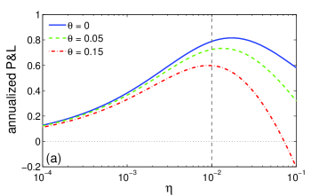
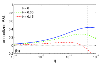
Figure 4: Net annualized risk adjusted P&L, $\sqrt{255}~{}\frac{\langle\delta{\mathcal{P}}_{\infty}\rangle-\langle{\mathcal{T}}_{\infty}\rangle}{\sqrt{v_{\infty}}}$, as a function of the strategy timescale $\eta$, for the market with $\beta_{0}=0.1$, and (a) long-term correlations ($\lambda=0.01$) and (b) short-time correlation ($\lambda=0.05$). Three curves correspond to different transaction costs $\theta$: $0$ (solid blue), $0.05$ (dashed green) and $0.15$ (dash-dotted red). Vertical black line indicates $\lambda$.

3.3 Skewness and kurtosis

In principle, one can compute explicitly the other cumulant moments and access skewness and kurtosis of the cumulative P&L. However, these expressions become too lengthy for practical use. In turn, the general matrix formula (21) allows for rapid numerical computation of these quantities. Figure 5 shows skewness ($\kappa_{3}/\kappa_{2}^{3/2}$) and kurtosis ($\kappa_{4}/\kappa_{2}^{2}$) of the cumulative P&L, ${\mathcal{P}}_{t,t_{0}}$, as functions of the lag time $t$. Both quantities exhibit a maximum at $t\approx 1/\eta$, i.e., the timescale of trend following strategy. In other words, the strategy induces auto-correlations of P&Ls that are significant up to time $1/\eta$ and then slowly decay. In fact, if incremental P&Ls, $\delta{\mathcal{P}}_{t_{0}+1}$, … , $\delta{\mathcal{P}}_{t_{0}+t}$, were independent and identically distributed, the skewness and kurtosis of their sum, ${\mathcal{P}}_{t,t_{0}}$, would decay as $1/\sqrt{t}$ and $1/t$, respectively. We emphasize that this behavior of $\delta{\mathcal{P}}_{t}$ is induced by the trend following strategy itself, irrespectively of auto-correlations of returns. This is confirmed by the fact that both skewness and kurtosis behave similarly for independent and auto-correlated returns.

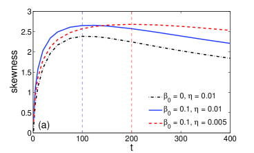
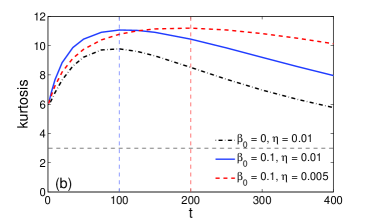
Figure 5: (a) Skewness, $\kappa_{3}/\kappa_{2}^{3/2}$, and (b) kurtosis, $\kappa_{4}/\kappa_{2}^{2}$, of the cumulative P&L, ${\mathcal{P}}_{t,t_{0}}$ (with $t_{0}=200$ and two timescales, $\eta_{1}=0.01$ and $\eta_{2}=0.005$), for auto-correlated returns ($\beta_{0}=0.1$ and $\lambda=0.01$) and independent returns ($\beta_{0}=0$). Two vertical dashed lines indicate $1/\eta_{1}$ and $1/\eta_{2}$, while horizontal dashed line locates the level of kurtosis (equal to $3$) of Gaussian distribution.

3.4 Distribution of incremental P&L

According to Eq. (17), the incremental P&L, $\delta{\mathcal{P}}_{{\bar{t}}}$, is the quadratic form defined by the symmetric matrix ${\bf M}_{1-\eta}^{(1,{\bar{t}}-1)}$ from Eq. (16). The probability distribution of $\delta{\mathcal{P}}_{\bar{t}}$ can therefore be determined through the inverse Fourier transform (19).

3.4.1 Independent returns

We first consider the case of independent returns ($\beta_{0}=0$), for which the covariance matrix is trivial: ${\bf C}={\bf I}$. In that case, there are only two nonzero eigenvalues of the matrix ${\bf M}{\bf C}={\bf M}_{1-\eta}^{(1,{\bar{t}}-1)}$,

$$\mu_{\pm}=\pm\gamma~{}\sqrt{\frac{1-(1-\eta)^{2({\bar{t}}-1)}}{1-(1-\eta)^{2}}}=\pm\sqrt{1-(1-\eta)^{2({\bar{t}}-1)}},$$ (32)

where Eq. (29) was used in the last relation. As a consequence, the characteristic function of the incremental P&L is $\phi(k)=(1+k^{2}\mu_{+}^{2})^{-1/2}$, from which the inverse Fourier transform yields

$$p(z)=\frac{K_{0}(|z|/\mu_{+})}{\pi\mu_{+}},$$ (33)

where $K_{0}(x)$ is the modified Bessel function of the second kind. For large $|z|$, the asymptotic behavior is

$$p(z)\simeq\frac{\exp(-|z|/\mu_{+})}{\sqrt{2\pi\mu_{+}|z|}}\bigl{(}1+O(1/|z|)\bigr{)}\qquad(|z|\to\infty).$$ (34)

Note that $\mu_{+}^{2}$ is the variance of the incremental P&L. The skewness and kurtosis are $0$ and $6$, respectively (see Fig. 5, on which an incremental P&L corresponds to $t=1$). In the stationary limit $t_{0}\to\infty$, one gets $\mu_{+}=1$.

Figure 6 compares the probability density $p(z)$ of the incremental P&L, $\delta{\mathcal{P}}_{\bar{t}}$, with the Gaussian density $(2\pi)^{-1/2}\exp(-z^{2}/2)$ of a single return $r_{\bar{t}}$ (with the unit variance). Although the mean and variance of these two distributions are identical, their overall behaviors are drastically different. The incremental P&L is peaked at $0$ (in fact, $K_{0}(z)$ logarithmically diverges at $0$), while the tail decay is much slower than for returns. This transformation from a Gaussian density to $p(z)$ is the effect of a trend following strategy.

3.4.2 Auto-correlated returns

For auto-correlated returns ($\beta_{0}\neq 0$), the diagonalization of the matrix ${\bf M}{\bf C}$ and computation of the probability density $p(z)$ can be performed numerically. As illustrated on Fig. 6, small auto-correlations of returns ($\beta_{0}=0.1$) slightly modify the probability distribution (33) by shifting the mean $\langle\delta{\mathcal{P}}_{t}\rangle$ from zero to a small positive value and by increasing the probability of extreme values of $\delta{\mathcal{P}}_{t}$ (both positive and negative tails).

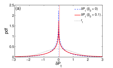
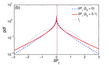
Figure 6: Probability distribution of the incremental P&L, $\delta{\mathcal{P}}_{\bar{t}}$ (${\bar{t}}=200$ and $\eta=0.01$), for independent returns (dashed blue line, $\beta_{0}=0$, Eq. (33)) and for auto-correlated returns (solid red line, $\beta_{0}=0.1$, $\lambda=0.01$): (a) linear scale, (b) semi-logarithmic scale. The Gaussian distribution of returns $r_{\bar{t}}$ is plotted for comparison (dotted black line). Vertical lines indicate the mean value $\langle\delta{\mathcal{P}}_{\bar{t}}\rangle$ for both cases (note that the variance of $\delta{\mathcal{P}}_{\bar{t}}$ is equal to $1$ for independent returns and to $1.01$ for auto-correlated returns).

3.5 Distribution of cumulative P&L

The probability distribution of the cumulative P&L, ${\mathcal{P}}_{t,t_{0}}$, can be obtained numerically through the inverse Fourier transform (19). Figure 7 shows the probability density $p(z)$ of ${\mathcal{P}}_{t,t_{0}}$ for independent returns ($\beta_{0}=0$) and for auto-correlated returns (with $\beta_{0}=0.1$ and $\lambda=0.01$). The initiation period of $t_{0}=200$ points was ignored to achieve stationary properties. In sharp contrast to symmetric (or almost symmetric) distributions of the incremental P&L from Fig. 6, the distribution of the cumulative P&L is strongly skewed and asymmetric, even for independent returns, in agreement with earlier observations [12, 13]. The most probable P&L is negative, while the mean $\langle{\mathcal{P}}_{t,t_{0}}\rangle$ is nonnegative (it is $0$ for $\beta_{0}=0$ and strictly positive for $\beta_{0}\neq 0$). The positive mean P&L for $\beta_{0}\neq 0$ is ensured by relatively large probability for getting large positive profits. This result agrees with earlier observations that trend followers experience often small losses, waiting for a trend that may lead to considerable profits [12]. We emphasize again that skewness of ${\mathcal{P}}_{t,t_{0}}$ emerges due to the trading strategy itself, irrespectively of auto-correlations of returns.

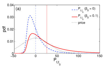
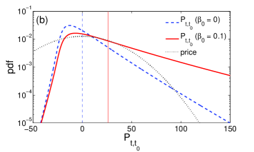
Figure 7: Probability distribution of the cumulative P&L, ${\mathcal{P}}_{t,t_{0}}$ ($t=300$, $t_{0}=200$, and $\eta=0.01$), for independent returns (dashed blue line, $\beta_{0}=0$) and for auto-correlated returns (solid red line, $\beta_{0}=0.1$, $\lambda=0.01$): (a) linear scale, (b) semi-logarithmic scale. The Gaussian distribution of price variation, $r_{t_{0}+1}+...+r_{t_{0}+t}$, is plotted for comparison (dotted black line). Vertical lines indicate the mean value $\langle{\mathcal{P}}_{t,t_{0}}\rangle$ for both cases.

3.6 Quantiles

Inspecting the distribution on Fig. 7, one can clearly observe an exponential decay of both positive and negative tails, in agreement with the expected asymptotic behavior (20). Importantly, the decay of the probability of negative P&Ls is much steeper than that of positive P&Ls. These extreme events can be characterized by quantiles. For this purpose, one first integrates the density $p(z)$ to get the cumulative probability distribution $F(z)$ and then solves the equation $F(z_{q})=q$ with $0<q<1$ that determines the $q$-quantile $z_{q}$ of the distribution. In a first approximation, power law corrections in Eq. (20) can be ignored (by setting $\nu_{\pm}=0$) so that

$$\begin{split}F(z)&\approx A_{-}|\mu_{-}|\exp(-z/\mu_{-})\hskip 15.649pt(z\to-\infty),\\ 1-F(z)&\approx A_{+}\mu_{+}\exp(-z/\mu_{+})\qquad(z\to\infty).\\ \end{split}$$

Extreme negative values of the cumulative P&L correspond to the limit $q\to 0$ for which the equation $F(z_{q})=q$ can be approximately solved as

$$z_{q}\approx-|\mu_{-}|\ln\left(\frac{A_{-}|\mu_{-}|}{q}\right)\qquad(q\to 0).$$ (35)

As expected, the behavior of the small $q$-quantile $z_{q}$ is essentially determined by the smallest eigenvalue $\mu_{-}$ of the matrix ${\bf M}{\bf C}$. In turn, extreme positive values of P&L correspond to the limit $q\to 1$ for which

$$z_{q}\approx\mu_{+}\ln\left(\frac{A_{+}\mu_{+}}{1-q}\right)\qquad(q\to 1).$$ (36)

The large $q$-quantile is therefore mainly determined by the largest eigenvalue $\mu_{+}$ of the matrix ${\bf M}{\bf C}$.

The behavior of the smallest and the largest eigenvalues $\mu_{\pm}$ of the matrix ${\bf M}_{1-\eta}^{(t,t_{0})}{\bf C}$ for the cumulative P&L is illustrated on Fig. 8. The largest eigenvalue $\mu_{+}$ grows with time $t$ and slowly approaches a constant value at long $t$. In turn, the smallest eigenvalue $\mu_{-}$ decreases and approaches a constant value much faster. For independent returns, we compute in C the asymptotic values $\mu_{\pm}^{\infty}$:

$$\mu_{+}^{\infty} = \frac{2\sqrt{\eta(2-\eta)}}{\eta}\approx\frac{\sqrt{8}}{\sqrt{\eta}},$$ (37)

$$\mu_{-}^{\infty} = -\frac{\sqrt{\eta(2-\eta)}}{2\eta(1-\eta)(2-\eta)}\approx-\frac{1}{\sqrt{8\eta}}.$$ (38)

These values are shown on Fig. 8b by horizontal dash-dotted lines. One can see that $\mu_{+}^{\infty}$ is 8 times larger than $|\mu_{-}^{\infty}|$. Most importantly, Eq. (38) turns out to be an accurate approximation for the smallest eigenvalue $\mu_{-}$ even for auto-correlated returns. In other words, extreme negative P&Ls weakly depend on the market features (here, $\beta_{0}$ and $\lambda$) and are mainly determined by the trend following strategy (timescale $\eta$). In turn, the largest eigenvalue $\mu_{+}$ for auto-correlated returns may attain much larger values than $\mu_{+}^{\infty}$ from Eq. (37). In other words, the presence of trends due to auto-correlations of returns increases $\mu_{+}$ and thus enhances the probability of extreme positive P&Ls. In contrast to $\mu_{-}$, the largest eigenvalue $\mu_{+}$ is sensitive to the market features.

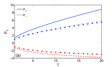
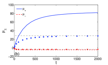
Figure 8: The largest and the smallest eigenvalues of the matrix ${\bf M}_{1-\eta}^{(t,t_{0})}{\bf C}$ (with $t_{0}=200$, $\eta=0.01$), for independent returns (symbols) and for auto-correlated returns (lines, $\beta_{0}=0.1$, $\lambda=0.01$). (a) Short-time behavior. Black dash-dotted lines indicate the asymptotic behavior (39). (b) Long-time behavior. Horizontal black dash-dotted lines indicate the asymptotic values $\mu_{\pm}^{\infty}$ from Eqs. (37, 38).

We also analyzed the behavior of the largest and the smallest eigenvalues $\mu_{\pm}$ in the opposite case of short times $t$. For independent returns, we compute in [30] the eigenvalues of the matrix ${\bf M}_{1-\eta}^{(t,t_{0})}{\bf C}$ for $t=2,3,4$ and $t_{0}\to\infty$. These explicit results suggest the conjectural asymptotic relation

$$\mu_{\pm}\simeq\pm\sqrt{t}+(t-1)\sqrt{\eta/2}+O(\eta),$$ (39)

which is applicable for small $\eta$ and moderate values of $t$ (see Fig. 8a). At short times, the small $q$-quantile can be approximated as

$$z_{q}\approx-\sqrt{t}\biggl{(}1-\frac{t-1}{\sqrt{2t}}\sqrt{\eta}\biggr{)}\ln\left(\frac{A_{-}\sqrt{t}}{q}\right)\qquad(q\to 0).$$ (40)

This behavior can be compared to the quantile of price variation over the time $t$, $r_{t_{0}+1}+...+r_{t_{0}+t}$. For independent returns, this is a Gaussian variable with mean zero and variance $t$, independently of the initiation period duration $t_{0}$. The cumulative probability distribution is $\frac{1}{2}(1+{\rm erf}(z/\sqrt{2t}))$, from which the $q$-quantile is given by the inverse error function:

$$z_{q}^{0}=2\sqrt{t}~{}{\rm erf}^{-1}(2q-1).$$ (41)

One can see that this quantile grows as $\sqrt{t}$, while $z_{q}^{0}/\sqrt{t}$ is constant. In turn, the quantile for the P&L, even after normalization by $\sqrt{t}$, exhibits a power law increase according to Eq. (40).

3.6.1 Auto-correlated returns

For auto-correlated returns ($\beta_{0}\neq 0$), the quantiles were computed numerically by solving the equation $F(z_{q})=q$, in which the cumulative probability distribution $F(z)$ was found by integrating the probability density $p(z)$.

Figure 9 illustrates the behavior of quantiles for the cumulative P&L, ${\mathcal{P}}_{t,t_{0}}$, and for price variation over the same time $t$, $r_{t_{0}+1}+...+r_{t_{0}+t}$. For independent returns ($\beta_{0}=0$), the Gaussian quantile grows as $\sqrt{t}$ according to Eq. (41). In turn, the quantiles for ${\mathcal{P}}_{t,t_{0}}$ exhibit quite different behavior showing a strong asymmetry between positive and negative values. This asymmetry is further enhanced by auto-correlations of returns. The most interesting feature is the behavior of the renormalized quantile $z_{q}/\sqrt{t}$ for small $q=0.01$ illustrated on Fig. 9d. At short time $t$, the negative values of this quantile are smaller for P&L than for price variation. In other words, a trend following strategy may lead to more significant losses than one could naively anticipate from a Gaussian distribution of price variations. At larger times, the situation changes to the opposite: the quantile for the P&L exceeds that for price variation quite significantly. In other words, the trend following strategy ensures smaller losses at longer times, even in the absence of trends (when $\beta_{0}=0$, see Fig. 9a,c).

One can also observe many similarities between Fig. 2a,b (Dow Jones) and Fig. 9a,b (present model). In particular, the $1\%$ quantiles in both cases are close to each other, confirming that quantiles for extreme negative P&Ls weakly depend on market features and may be well approximated even by a simple model. In turn, the $99\%$ quantiles on Fig. 2b and Fig. 9b are not so close, i.e., quantiles for extreme positive P&Ls are sensitive to market features.

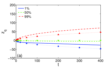
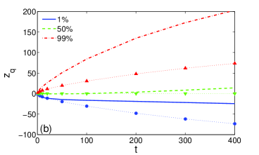
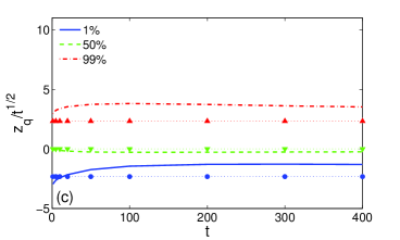
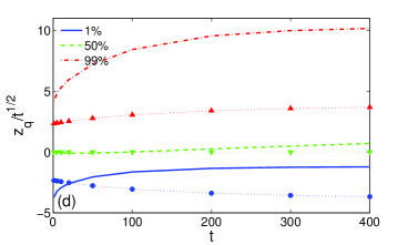
Figure 9: Quantiles $z_{0.01}$, $z_{0.5}$ and $z_{0.99}$ ($1\%$, $50\%$, and $99\%$) of the cumulative P&L, ${\mathcal{P}}_{t,t_{0}}$ as functions of time $t$, with $\eta=0.01$ and $t_{0}=200$: (a) for independent returns ($\beta_{0}=0$), and (b) auto-correlated returns ($\beta_{0}=0.1$, $\lambda=0.01$). The same quantiles of price variation over time $t$, $r_{t_{0}+1}+...+r_{t_{0}+t}$, are shown by symbols. Since Gaussian quantiles grow as $\sqrt{t}$, the ratio $z_{q}/\sqrt{t}$ is also plotted for independent returns (c) and for auto-correlated returns (d), with the same parameters.

4 Conclusion

In this paper, we investigated how price variations of a stock are transformed into profits and losses of a trend following strategy. We started by deriving simple formulas for the mean and variance of the P&L, as well as the mean turnover of the strategy. The explicit expression for the net annualized risk adjusted P&L allowed us to analyze the profitability of trend following strategies in the presence of auto-correlations and transaction costs, and their sensitivity to the choice of parameters. We next proceeded in computing explicitly the probability distribution of P&L and investigating its asymptotic behavior. The theoretical analysis was mainly done for independent returns and confronted to numerical results for auto-correlated returns. Although the model of correlated returns was over-simplified, it allowed us to illustrate the basic features and mechanisms of a trend following strategy. Moreover, the general matrix formulas provided at the beginning of Sec. 3 are applicable to arbitrary Gaussian models.

It is worth emphasizing that quantitative results of this study are model dependent. For instance, we analyzed the asymptotic behavior of the probability density $p(z)$ for extreme losses and showed its exponential decay with the rate $\mu_{-}^{\infty}\approx-1/\sqrt{8\eta}$. An exponential decay is a universal feature for quadratic forms of Gaussian vectors. However, the dependence of the smallest eigenvalue $\mu_{-}$ on the parameter $\eta$ was only derived for the studied trend following strategy. Moreover, the unknown prefactor $A_{-}$ in the asymptotic formula (20) and related quantiles may strongly depend on other parameters, rendering quantitative estimates of quantiles model dependent. Finally, the asymptotic exponential decay of $p(z)$ may settle at extremely large values of $|z|$, at which the probability density is negligible and out of practical interest. At the same time, qualitative conclusions of the study are expected to be general. In fact, a trend following strategy strongly modifies probabilistic properties of price time series, yielding skewed asymmetric distributions, with often small losses and less frequent high profits. The probability of extreme losses decays much faster than the probability of extreme profits. Moreover, the occurence of extreme losses is more influenced by the trend following strategy than by the market itself. In turn, the occurence of extreme profits depends on both the strategy and the market. We showed that the usual Gaussian paradigm may lead to erroneous conclusions about trend following strategies. For instance, at short times, trend following strategies admit larger losses than one may anticipate from standard Gaussian estimates. This is an important message for systematic traders and risk analysts.

The present analysis can be extended to arbitrary Gaussian models of returns and to multiple correlated stocks. The practical advantage of choosing linear equation (13) is that the signal from EMAs of individual stocks is simply the sum of the related signals. As a consequence, the P&L of a portfolio is again a quadratic form of Gaussian vectors for which general matrix formulas at the beginning of Sec. 3 are still applicable. One can therefore study the role of inter-stock correlations which may significantly improve risk control of trend following strategies.

Appendix A Mean turnover of trend following strategy

Accounting for transaction costs is important for a comprehensive analysis of trading strategies. We define the daily turnover of the trend following strategy as

$${\mathcal{T}}_{t}=\theta~{}|s_{t}-s_{t-1}|^{\alpha},$$ (42)

where $\theta$ represents transaction cost, and $\alpha$ is an appropriate exponent (typically $\alpha=1$ or $\alpha=2$). The mean turnover can be evaluated by using the identity

$$\langle f\bigl{(}({\bf r}^{\dagger}{\bf a})\bigr{)}\rangle=\int\limits_{-\infty}^{\infty}dz~{}f(z)~{}\frac{1}{\sqrt{2\pi({\bf a}^{\dagger}{\bf C}{\bf a})}}\exp\left(-\frac{z^{2}}{2({\bf a}^{\dagger}{\bf C}{\bf a})}\right),$$ (43)

where $f(z)$ is a continuous function of the scalar product $({\bf r}^{\dagger}{\bf a})$, ${\bf r}$ is a Gaussian vector with mean zero and covariance matrix ${\bf C}$, and ${\bf a}$ is a fixed vector. Setting $f(z)=|z|^{\alpha}$ and $a_{j}=\gamma\bigl{[}({\bf E}_{1-\eta})_{t,j}-({\bf E}_{1-\eta})_{t-1,j}\bigr{]}$, one gets

$$\begin{split}\langle{\mathcal{T}}_{t}\rangle&=\theta~{}\frac{\Gamma(\frac{1+\alpha}{2})}{\sqrt{\pi}}\bigl{[}2({\bf a}^{\dagger}{\bf C}{\bf a})\bigr{]}^{\alpha/2}=\theta~{}\frac{\Gamma(\frac{1+\alpha}{2})}{\sqrt{\pi}}(2\gamma^{2})^{\alpha/2}\\ &\times\left(\bigl{[}{\bf E}_{p}{\bf C}{\bf E}_{p}^{\dagger}\bigr{]}_{t,t}-2\bigl{[}{\bf E}_{p}{\bf C}{\bf E}_{p}^{\dagger}\bigr{]}_{t,t-1}+\bigl{[}{\bf E}_{p}{\bf C}{\bf E}_{p}^{\dagger}\bigr{]}_{t-1,t-1}\right)^{\alpha/2},\\ \end{split}$$ (44)

where $\Gamma(z)$ is Gamma function. Using Eq. (5), one obtains explicitly

$$\begin{split}&\langle{\mathcal{T}}_{t}\rangle=\theta~{}\frac{\Gamma(\frac{1+\alpha}{2})}{\sqrt{\pi}}(2\gamma^{2})^{\alpha/2}\biggl{(}\frac{2-(1-p)p^{2t-4}}{1+p}+\frac{\beta_{0}^{2}(1-q^{2})}{(1-pq)(p-q)}\biggl{[}\frac{2(p-q)}{(1+p)(1+q)}\\ &-\frac{(1-p)p^{2t-3}}{1+p}+\frac{(1-q)q^{2t-3}}{1+q}-\frac{(p^{t-1}-p^{t-2}-q^{t-1}+q^{t-2})^{2}}{p-q}\biggr{]}\biggr{)}^{\alpha/2}.\\ \end{split}$$ (45)

In the special case $p=q$, one gets

$$\begin{split}\langle{\mathcal{T}}_{t}\rangle&=\theta~{}\frac{\Gamma(\frac{1+\alpha}{2})}{\sqrt{\pi}}(2\gamma^{2})^{\alpha/2}\biggl{(}\frac{2-(1-q)q^{2t-4}}{1+q}\\ &+\frac{\beta_{0}^{2}}{(1+q)^{2}}\biggl{[}2-q^{2t-4}\biggl{(}1+\bigl{[}(q^{-1}-q)(t-2)-1\bigr{]}^{2}\biggr{)}\biggr{]}\biggr{)}^{\alpha/2}.\\ \end{split}$$ (46)

In the stationary limit, one finds

$$\langle{\mathcal{T}}_{\infty}\rangle=\theta~{}\frac{\Gamma(\frac{1+\alpha}{2})}{\sqrt{\pi}}(2\gamma^{2})^{\alpha/2}\biggl{(}\frac{2}{1+p}+\frac{2\beta_{0}^{2}(1-q^{2})}{(1-pq)(1+p)(1+q)}\biggr{)}^{\alpha/2}$$ (47)

that simplifies when $\lambda\ll 1$ and $\eta\ll 1$ to

$$\langle{\mathcal{T}}_{\infty}\rangle\approx\theta~{}\frac{\Gamma(\frac{1+\alpha}{2})2^{\alpha}}{\sqrt{\pi}}\biggl{(}\eta+\frac{\beta_{0}^{2}\lambda\eta}{\lambda+\eta}\biggr{)}^{\alpha/2}\approx\theta~{}\frac{\Gamma(\frac{1+\alpha}{2})2^{\alpha}}{\sqrt{\pi}}~{}\eta^{\alpha/2}.$$ (48)

Appendix B Variogram of incremental P&L

We sketch the derivation of the variogram of incremental P&Ls in the stationary limit $t_{0}\to\infty$. The variogram is defined as

$$V_{t,t_{0}}^{\textrm{P\&L}}=\frac{{\rm var}\{\delta{\mathcal{P}}_{t_{0}+1}+...+\delta{\mathcal{P}}_{t_{0}+t}\}}{{\rm var}\{\delta{\mathcal{P}}_{t_{0}+1}\}+...+{\rm var}\{\delta{\mathcal{P}}_{t_{0}+t}\}}.$$ (49)

The variances ${\rm var}\{\delta{\mathcal{P}}_{k}\}$ in the denominator are given by Eq. (27). One can explicitly compute their sum for $k$ ranging from $t_{0}+1$ to $t_{0}+t$ and then take the limit $t_{0}\to\infty$. As expected, this limit is simply equal $tv_{\infty}$, where the stationary variance $v_{\infty}$ is given by Eq. (28). The major difficulties rely in the computation of the numerator of Eq. (49) which contains correlations between incremental P&Ls.

We start by writing the definition of the variance

$$\begin{split}{\rm var}\{\delta{\mathcal{P}}_{t_{0}+1}+...+\delta{\mathcal{P}}_{t_{0}+t}\}&=\sum\limits_{j,k=t_{0}+1}^{t_{0}+t}\bigl{[}\langle r_{j}s_{j}r_{k}s_{k}\rangle-\langle r_{j}s_{j}\rangle\langle r_{k}s_{k}\rangle\bigr{]}\\ &=\sum\limits_{j,k=t_{0}+1}^{t_{0}+t}\bigl{[}\langle r_{j}r_{k}\rangle\langle s_{j}s_{k}\rangle+\langle r_{j}s_{k}\rangle\langle r_{k}s_{j}\rangle\bigr{]},\\ \end{split}$$ (50)

where the second relation implied by the Wick’s theorem. Lengthy but straightforward computation yields

$$\begin{split}\langle s_{j}s_{k}\rangle&=p^{|j-k|}-p^{j+k-2}+\beta_{0}^{2}\biggl{(}\frac{p(1-q^{2})}{(1-pq)(p-q)}(p^{|j-k|}-p^{j+k-2})\\ &-\frac{q(1-p^{2})}{(1-pq)(p-q)}\bigl{[}p^{j+k-2}+q^{|j-k|}-p^{j-1}q^{k-1}-p^{k-1}q^{j-1}\bigr{]}\\ &-\frac{1-p^{2}}{(p-q)^{2}}(p^{j-1}-q^{j-1})(p^{k-1}-q^{k-1})\biggr{)}\\ \end{split}$$

and

$$\frac{\langle r_{j}s_{k}\rangle}{\gamma\beta_{0}^{2}}=\begin{cases}\frac{p^{k-j-1}}{\beta_{0}^{2}}+p^{k-j-1}\frac{1-(pq)^{j}}{1-pq}+q\frac{p^{k-j-1}-q^{k-j-1}}{p-q}-q^{j-1}\frac{p^{k-1}-q^{k-1}}{p-q}\quad(k>j),\cr q^{j-k+1}\frac{1-(pq)^{k-1}}{1-pq}-q^{j-1}\frac{p^{k-1}-q^{k-1}}{p-q}\hskip 130.88268pt(k\leq j).\end{cases}$$

The numerator of Eq. (49) is then obtained by computing the double sum in Eq. (50). Since we are interested in the stationary limit $t_{0}\to\infty$, it is sufficient to keep only the terms with $j-k$, in which the dependence on $t_{0}$ is canceled. In the stationary limit, one gets the following variance

$$\begin{split}&\lim\limits_{t_{0}\to\infty}{\rm var}\{\delta{\mathcal{P}}_{t_{0}+1}+...+\delta{\mathcal{P}}_{t_{0}+t}\}=\biggl{[}1+2\beta_{0}^{2}\frac{1+q^{2}-2p^{2}q^{2}}{(1-pq)^{2}}+\beta_{0}^{4}c_{2}\biggr{]}t\\ &-2\beta_{0}^{2}q\frac{p+q-2p^{2}q}{(1-pq)^{3}}\biggl{[}1+\beta_{0}^{2}\frac{p(1-q^{2})}{(1-pq)(p-q)}\biggr{]}\bigl{(}1-(pq)^{t}\bigr{)}\\ &+\frac{4\beta_{0}^{4}q^{3}(1-p^{2})}{(1-pq)(p-q)(1-q^{2})^{2}}\bigl{(}1-q^{2t}\bigr{)},\\ \end{split}$$ (51)

where

$$c_{2}=\frac{2p^{3}q^{5}+2p^{3}q^{3}-6p^{2}q^{2}+2q^{4}p^{2}-4q^{3}p-q^{5}p+pq+1-q^{4}+4q^{2}}{(1-q^{2})(1-pq)^{3}}.$$

For the special case $p=q$, one gets

$$\begin{split}&\lim\limits_{t_{0}\to\infty}{\rm var}\{\delta{\mathcal{P}}_{t_{0}+1}+...+\delta{\mathcal{P}}_{t_{0}+t}\}=\biggl{[}1+2\beta_{0}^{2}\frac{1+2q^{2}}{1-q^{2}}+\beta_{0}^{4}\frac{1+7q^{2}+2q^{4}}{(1-q^{2})^{2}}\biggr{]}t\\ &-\frac{4\beta_{0}^{2}q^{2}}{(1-q^{2})^{2}}\biggl{[}1+\beta_{0}^{2}\frac{2q^{2}+3/2}{1-q^{2}}\biggr{]}(1-q^{2t})+\frac{4\beta_{0}^{4}q^{2}}{(1-q^{2})^{2}}~{}q^{2t}~{}t.\\ \end{split}$$

Dividing Eq. (51) by $tv_{\infty}$, one gets the variogram $V_{t,\infty}^{\textrm{P\&L}}$. This expression can be compared to the variogram of returns from Eq. (9). Both variograms behave similarly, exhibiting both rapid exponential decay and slow power law decay. The asymptotic value of the variogram $V_{t,\infty}^{\textrm{P\&L}}$ as $t\to\infty$ is

$$V_{\infty,\infty}^{\textrm{P\&L}}=\frac{1+2\beta_{0}^{2}\frac{1+q^{2}-2p^{2}q^{2}}{(1-pq)^{2}}+\beta_{0}^{4}c_{2}}{1+\frac{2\beta_{0}^{2}}{1-pq}+\frac{\beta_{0}^{4}(1+q^{2}-2p^{2}q^{2})}{(1-pq)^{2}}}.$$ (52)

In the special case $p=q=1-\lambda$, one gets for $\lambda\ll 1$ and $\beta_{0}\ll 1$

$$V_{\infty,\infty}^{\textrm{P\&L}}\approx 1+\frac{2\beta_{0}^{2}}{\lambda}+\frac{(\beta_{0}^{2}/\lambda)^{2}}{2(1+\beta_{0}^{2}/\lambda)}.$$ (53)

For comparison, the variogram of returns from Eq. (9) gets the asymptotic value $1+2\beta_{0}^{2}/\lambda$. It is worth noting that $\beta_{0}^{2}/\lambda$ does not need to be a small parameter.

Appendix C The largest and the smallest eigenvalues at long times

We present explicit formulas for the eigenvalues of the matrix ${\bf M}{\bf C}$ determining the cumulative P&L for independent returns at long times. In that case, ${\bf M}{\bf C}={\bf M}_{1-\eta}^{(t,t_{0})}$. We first consider the simpler case when an initiation period is not ignored (i.e., $t_{0}=0$). In the limit $t\to\infty$, the matrix ${\bf M}_{1-\eta}^{(t,0)}=\gamma[{\bf E}_{1-\eta}+{\bf E}_{1-\eta}^{\dagger}]$ becomes close to a cyclic matrix whose eigenvalues can be computed as

$$\mu_{1-\omega}=\gamma\sum\limits_{j=1}^{\infty}|p|^{j-1}\bigl{[}e^{i\pi j\omega}+e^{i\pi j\omega}\bigr{]}=2\gamma\frac{\cos(\pi\omega)-p}{1-2p\cos(\pi\omega)+p^{2}},$$ (54)

where $\omega\in[0,1]$ is the “index”, and $p=1-\eta$. The largest eigenvalue of the limiting matrix is then

$$\mu_{+}^{\infty}=\mu_{\omega=1}=\frac{2\gamma}{\eta},$$ (55)

while the smallest eigenvalue is $\mu_{\omega=0}=-\frac{\gamma}{1-\eta/2}$.

When $t_{0}>0$, discarding the first $t_{0}$ points corresponds to setting the block of size $t_{0}\times t_{0}$ of the matrix ${\bf M}_{1-\eta}^{(t,0)}$ to zero. This modification introduces $t_{0}$ zero eigenvalues into the spectrum and also changes the smallest eigenvalue $\mu_{-}$ which becomes significantly smaller than $\mu_{\omega=0}$. In what follows, we compute the smallest eigenvalue $\mu_{-}$ in the double limit $t_{0}\to\infty$ and $t\to\infty$. For this purpose, we first guess the corresponding eigenvector ${\bf U}$ and then justify explicitly the correctness of the guess. We take the vector ${\bf U}$ of the form:

$${\bf U}=\bigl{(}\underbrace{p^{t_{0}-1},p^{t_{0}-2},...,p,1}_{t_{0}~{}\textrm{elements}},-a,-a\tilde{p},-a\tilde{p}^{2},...\bigr{)}^{\dagger},$$

where $a$ and $\tilde{p}$ are two parameters to be determined. Applying the matrix ${\bf M}_{1-\eta}^{(t,t_{0})}$ to this vector, one gets

$${\bf M}_{1-\eta}^{(t,t_{0})}{\bf U}=\gamma\left(\begin{array}[]{c}-ap^{t_{0}-1}(1+p\tilde{p}+...)\\ -ap^{t_{0}-2}(1+p\tilde{p}+...)\\ ...\\ -a(1+p\tilde{p}+...)\\ \hline\cr(1+p^{2}+...)-a(\tilde{p}[1+p\tilde{p}+...])\\ p(1+p^{2}+...)-a(1+\tilde{p}^{2}[1+p\tilde{p}+...])\\ ...\\ p^{k+1}(1+...)-a([p^{k}+p^{k-1}\tilde{p}+...+\tilde{p}^{k}]+\tilde{p}^{k+2}[1+...])\\ ...\\ \end{array}\right),$$

where the geometrical series $1+p\tilde{p}+(p\tilde{p})^{2}+...$ and $1+p^{2}+p^{4}+...$ contain infinitely many terms in the limits $t\to\infty$ and $t_{0}\to\infty$, respectively. If ${\bf U}$ is an eigenvector, the right hand side has to be identified with $\mu_{-}^{\infty}{\bf U}$. The first $t_{0}$ identities read $\mu_{-}^{\infty}=\frac{-a\gamma}{1-p\tilde{p}}$. The identity in the $(t_{0}+1)$-th row gives $-a\mu_{-}^{\infty}=\gamma[\frac{1}{1-p^{2}}-\frac{a\tilde{p}}{1-p\tilde{p}}]$, from which

$$\frac{a(a+\tilde{p})}{1-p\tilde{p}}=\frac{1}{1-p^{2}}.$$ (56)

Finally, an identity in the $(t_{0}+k+2)$-th row reads

$$-a\tilde{p}^{k+1}\mu_{-}^{\infty}=\gamma\biggl{[}\frac{p^{k+1}}{1-p^{2}}-a(p^{k}+p^{k-1}\tilde{p}+...+\tilde{p}^{k})-\frac{a\tilde{p}^{k+2}}{1-p\tilde{p}}\biggr{]},$$

from which one expresses $\tilde{p}=p-a(1-p^{2})$. Substituting this relation into Eq. (56), one gets $a=1/p$, from which $\tilde{p}=2p-1/p$ and finally

$$\mu_{-}^{\infty}=-\frac{\gamma}{2p(1-p^{2})}.$$ (57)

In this way, we constructed explicitly an eigenvalue $\mu_{-}^{\infty}$ and the corresponding eigenvector ${\bf U}$ of the limiting matrix ${\bf M}_{1-\eta}^{(\infty,\infty)}$. In turn, we did not show that $\mu_{-}^{\infty}$ is the smallest eigenvalue. Although the related demonstration could in principle be performed, this analysis is beyond the scope of the paper. We checked numerically that $\mu_{-}^{\infty}$ from Eq. (57) accurately approximates the smallest eigenvalue of the matrix ${\bf M}_{1-\eta}^{(t,t_{0})}$ for large enough $t_{0}$ and $t$.

References

• [1] M. W. Covel, Trend Following (Updated Edition): Learn to Make Millions in Up or Down Markets, Pearson Education, New Jersey, 2009.
• [2] A. F. Clenow, Following the Trend: Diversified Managed Futures Trading, Wiley & Sons, Chichester UK, 2013.
• [3] L. K. C. Chan, N. Jegadeesh, J. Lakonishok, J. Finance 51 (1996) 1681.
• [4] N. Jegadeesh, S. Titman, J. Finance 56 (2001) 699.
• [5] L. K. C. Chan, N. Jegadeesh, J. Lakonishok, Finan. Anal. J. 55 (1999) 80.
• [6] T. J. Moskowitz, Y. H. Ooi, L. H. Pedersen, J. Finan. Econ. 104 (2012) 228.
• [7] C. S. Asness, T. J. Moskowitz, L. H. Pedersen, J. Finance 68 (2013) 929.
• [8] N. Vandewalle, M. Ausloos, Phys. Rev. E 58 (1998) 6832.
• [9] N. Vandewalle, A. Ausloos, P. Boveroux, Physica A 269 (1999) 170.
• [10] A. Carbone, G. Castelli, H. E. Stanley, Phys. Rev. E 69 (2004) 026105.
• [11] S. Arianos, A. Carbone, C. Türk, Phys. Rev. E 84 (2011) 046113.
• [12] M. Potters, J.-P. Bouchaud, Wilmott Magazine (Jan 2006); online: ArXiv physics-0508104 (2005).
• [13] R. Martin, D. Zou, Momentum trading: ’skews me, Risk Magazine (2012).
• [14] T. G. Andersen, T. Bollerslev, F. X. Diebold, P. Labys, Multinat. Finance J. 4 (2000) 159.
• [15] J.-P. Bouchaud, M. Potters, Theory of Financial Risk and Derivative Pricing: From Statistical Physics to Risk Management, Cambridge University Press, 2003.
• [16] R. Mantegna, H. E. Stanley, An introduction to Econophysics, Cambridge University Press, Cambridge, 1999.
• [17] R. Mantegna, H. E. Stanley, Nature 376 (1995) 46.
• [18] Gabaix, Gopikrishnan, Plerou, Stanley, Nature 423 (2003) 267.
• [19] J.-P. Bouchaud, M. Potters, Physica A 299 (2001) 60.
• [20] D. Sornette, Phys. Rep. 378 (2003), 1.
• [21] J.-P. Bouchaud, Y. Gefen, M. Potters, M. Wyart, Quant. Finance 4 (2004) 176.
• [22] A. L. Stella, F. Baldovin, Pramana J. Phys. 71 (2008) 341.
• [23] J.-P. Bouchaud, A. Matacz, M. Potters, Phys. Rev. Lett. 87 (2001) 1.
• [24] S. Valeyre, D. S. Grebenkov, S. Aboura, Q. Liu, Quant. Finance (in press).
• [25] G. Box, G. M. Jenkins, G. C. Reinsel, Time Series Analysis: Forecasting and Control, Third ed., Prentice-Hall, 1994.
• [26] C. C. Holt, Office of Naval Research Memorandum 52 (1957); reprinted in Int. J. Forecast. 20 (2004) 5.
• [27] P. R. Winters, Management Science 6 (1960) 324.
• [28] R. G. Brown, Smoothing Forecasting and Prediction of Discrete Time Series, Englewood Cliffs, NJ: Prentice-Hall, 1963.
• [29] D. S. Grebenkov, Phys. Rev. E 84 (2011) 031124.
• [30] Supplementary Materials.