Gravitational Infall onto Molecular Filaments II. Externally Pressurized Cylinders

Abstract

In an extension of Fischera & Martin (2012a) and Heitsch (2013), two aspects of the evolution of externally pressurized, hydrostatic filaments are discussed. (a) The free-fall accretion of gas onto such a filament will lead to filament parameters (specifically, FWHM–column density relations) inconsistent with the observations of Arzoumanian et al. (2011), except for two cases: For low-mass, isothermal filaments, agreement is found as in the analysis by Fischera & Martin (2012b). Magnetized cases, for which the field scales weakly with the density as $B\propto n^{1/2}$, also reproduce observed parameters. (b) Realistically, the filaments will be embedded not only in gas of non-zero pressure, but also of non-zero density. Thus, the appearance of sheet-embedded filaments is explored. Generating a grid of filament models and comparing the resulting column density ratios and profile shapes with observations suggests that the three-dimensional filament profiles are intrinsically flatter than isothermal, beyond projection and evolution effects.

1. Motivation

In a previous study I explored the role of accretion for the evolution of an idealized filamentary molecular cloud (Heitsch, 2013, H13). For consistency with observed filament parameters, specifically with the discussion by Arzoumanian et al. (2011), the radial density profile was explicitly set, via

$$\rho(R)=\rho_{c}\left(1+\left(\frac{R}{R_{0}}\right)\right)^{-p/2},$$ (1)

with the core radius $R_{0}$ and the central density $\rho_{c}$. Herschel studies of filaments (Arzoumanian et al., 2011) determine the value of the exponent $p$ to be clearly less than the isothermal $p=4$ (Ostriker, 1964), though Hacar & Tafalla (2011) find steeper exponents consistent with $p=4$ in some cases for filaments in Taurus. Flatter than isothermal profiles have been ascribed to magnetic fields (Fiege & Pudritz, 2000a), accretion, and non-isothermality (Nakamura & Umemura, 1999). H13 was mainly interested in the effect of accretion on a filament’s evolution, but less in its structure. Yet, a more physical way to set $p$ would be desirable.

Fischera & Martin (2012a, FM12a) study the structure of infinite, externally pressurized cylinders and discuss how the filament profiles depend on the external pressure. They argue that for infinite overpressure (or, for the cylinder in a vacuum), the isothermal solution is recovered, while for finite pressures the profiles flatten, reaching lower $p$. They apply their models to a sample of four filaments (Fischera & Martin, 2012b, FM12b), finding good agreement with their isothermal cylinder model.

My goal here is to elucidate how the evolution of externally pressurized, isothermal cylinders depends on accretion, thus combining the analysis of FM12a and H13 (§2, 3). I will discuss isothermal, turbulent and magnetic cases. It also seems reasonable to explore the effect of ram pressure on the filament structure and evolution, since the infalling gas is expected to exert an additional pressure on the filament. I conclude with a tool to estimate the evolutionary stage of filaments embedded in flattened clouds (or sheets) in §4.

2. Evolution of an accreting, pressurized filament

The filament is modeled as an infinite, externally pressurized, and isothermal cylinder, accreting gas at free-fall velocities. Though free-fall accretion is certainly an extreme assumption (e.g. Miettinen, 2012), I intend it as a counter-point to the more classical equilibrium consideration.

2.1. Basic equations

The goal is to calculate the time evolution of the line mass $m$ due to accretion. For hydrostatic isothermal cylinders, radially stable solutions can only be found for

$$m<m_{cr}\equiv\frac{2c_{s}^{2}}{G}=16.3\left(\frac{T}{10\mbox{K}}\right)\,\mbox{M}_{\odot}\mbox{ pc}^{-1}$$ (2)

(e.g. Ostriker, 1964). Following FM12a, the line mass is given in terms of a criticality parameter,

$$f\equiv\frac{m}{m_{cr}}=\frac{mG}{2c_{s}^{2}}<1,$$ (3)

where $c_{s}$ is the isothermal sound speed. The core radius $R_{0}$ of equation 1 is set to the isothermal value,

$$R_{0}^{2}=\frac{m_{cr}}{\pi\rho_{c}}.$$ (4)

The mass accretion onto the filament can be described by

$$\frac{dm}{dt} = 2\pi R_{f}\rho_{ext}v_{R}$$ (5)

$$= 4\pi\rho_{ext}R_{f}\left(Gm(t)\,\ln\left(\frac{R_{ref}}{R_{f}}\right)\right)^{1/2},$$

where the steady-state, free-fall velocity around an infinite cylinder is given by

$$v_{R}=2\left(Gm\,\ln\frac{R_{ref}}{R}\right)^{1/2}.$$ (6)

(see Heitsch et al., 2009). In equation 5, $R_{f}$ is the filament radius, and $R_{ref}$ is a reference radius (actually, the integration constant), from which the fluid parcels start their travel to the filament (see discussion in H13, and §3.1.2). Thus, the accretion rate will depend on the evolutionary stage of the filament via the line mass $m(t)$, and on the filament radius $R_{f}$. The ambient density $\rho_{ext}$ is also a free parameter (see §2.2).

2.2. Boundary Conditions and Profiles

To determine $R_{f}$ and associated quantities, boundary conditions for the filament are needed. As do FM12a, I assume that the filament is embedded in a background medium of pressure $p_{ext}$, with the filament in pressure balance such that $p(R_{f})=p_{ext}$. To simplify the discussion, isothermality is assumed beyond the cylinder, and hence $\rho_{ext}=\rho(R_{f})$.

A brief summary of the results of FM12a can be found in Appendix A, including the expression for the filament radius

$$R_{f}=\sigma^{2}\left(\frac{2f(1-f)}{\pi Gp_{ext}}\right)^{1/2}$$ (7)

needed to evaluate equation 5. Here, $\sigma$ is a proxy for the effective sound speed. The goal is to consider a wider variety of physical environments, exploring their effect on the accretion and on observable filament parameters. Figure 1 summarizes the relevant physical quantities for all cases considered.

Before discussing each case in turn, this is as good a moment as any to point out differences in some of the diagnostic quantities with respect to H13. There, I compared the timescales for accretion and gravitational fragmentation with the result that accretion occurs on similar timescales as fragmentation, and thus should not be neglected when discussing the evolution of filaments. The expressions for the gravitational fragmentation time scale $\tau_{f}$ and maximum growth length scale $\lambda_{max}$ were taken from Tomisaka (1995), who in turn used the expressions of Nagasawa (1987),

$$\tau_{f} = \frac{2.95}{\sqrt{4\pi G\rho_{c}}}$$ (8)

$$\lambda_{max} = \frac{22.1c_{s}}{\sqrt{4\pi G\rho_{c}}}.$$ (9)

Yet, these expressions assume that the ambient pressure is zero. This assumption is no longer valid. FM12a calculated polynomial fits for $\tau_{f}$ and $\lambda_{max}$ (see their appendix E, equation E.1 and table E.1.). Note that I will use the same expressions for the magnetic cases, based on the argument that for axial magnetic fields, the longitudinal gravitational instability will be nearly unaffected, while the growth rates for varicose instabilities are substantially higher, and thus not of interest in our case (FM12a).

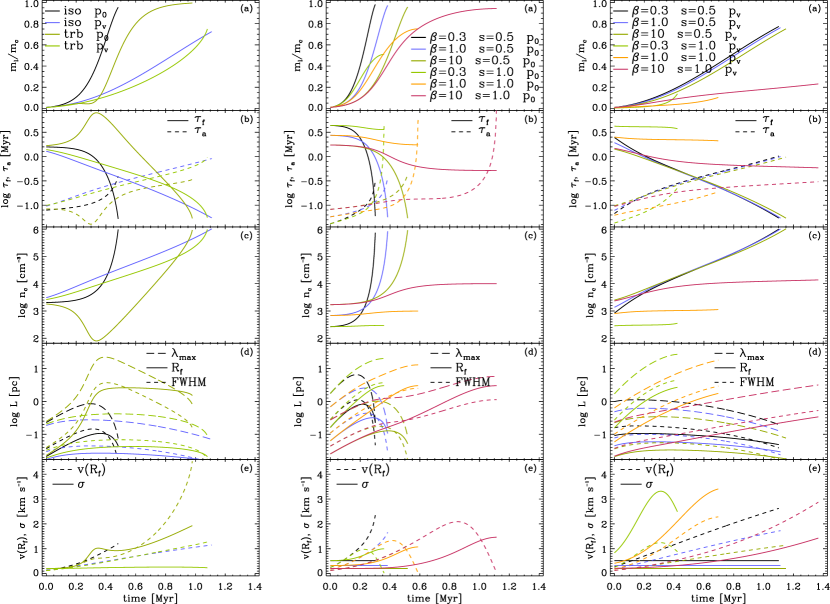
Figure 1.— Time evolution of filament parameters, for all cases considered (see text). From left to right: All isothermal and turbulent cases with constant and varying external pressure, all magnetic cases at constant pressure, all magnetic cases with varying external pressure. Each column has the following panels: (a) Line mass over critical value (eq. 2). (b) Fragmentation timescale $\tau_{f}$ (solid line) and accretion timescale $\tau_{a}$ (dashed line). (c) Central filament (atomic) density $n_{c}$ (eq. A3). (d) The filament radius $R_{f}$ (eq. 7) and the FWHM in parsec, and the wavelength of the most unstable mode (see text). (e) Accretion velocity $v(R_{f})$ (dashed line) and modified sound speed (solid line) $\sigma$ driven by accretion or magnetic fields.

2.2.1 The Isothermal Case

Equations 3, 5, and 7 result in an ordinary differential equation that can be integrated with a 4th order Runge-Kutta method. The RHS only depends on the line mass $m$. The left column of Figure 1 shows the results (black lines). For consistency with FM12a, I use $p_{ext}=2\times 10^{4}$ K cm^-3, and $T=10$ K, yielding identical results. Specifically, the FWHM peaks at $0.14$ pc. The FWHM is calculated numerically for the position $x=R_{FWHM}/R_{f}$ in the column density profile $N(0)/2=N(x)$, combining equations 15 and 18 of FM12a, with FWHM$=2R_{FWHM}$.

2.2.2 Effects of Ram Pressure

Since the filament is accreting mass, the infall could be thought to exert a ram pressure

$$p_{ram}=\rho_{ext}v_{R}^{2}=4\rho_{ext}\,G\,m\,\ln(R_{ref}/R_{f})$$ (10)

on the filament surface. Thus, the total external pressure is

$$p_{ext}=p_{ram}+p_{ext,0}$$ (11)

where $p_{ext,0}$ is the external thermal pressure. The accretion velocity $v_{R}$ for the isothermal case (left column, black lines) already suggests that the ram pressure could get substantially larger than the thermal pressure. Thus, the filament is “squeezed”, or, equivalently, truncated at smaller $R_{f}$, leading to an effective flattening of the profile, since $R_{f}<R_{0}$, see also Fig. 3 of FM12a. The radius $R_{f}$ now depends on the accretion velocity, and hence, in a non-trivial manner on itself. The numerical procedure is explained in Appendix B.1.

Blue lines in the left column of Figure 1 summarize the results. For the isothermal case with constant external pressure (§2.2.1), the accretion rate (eq. 5) increases with increasing filament radius $R_{f}$ and line mass $m$. Increasing the pressure (in our case by tracking the ram pressure $\rho_{ext}v_{R}^{2}$) reduces the filament radius, and thus the accretion rate. Thus, once $p_{ram}\approx p_{ext,0}$, the accretion rate drops below that of the constant pressure model, and thus the filament growth slows down. This can be seen in Figure 1(a), left column. The central densities end up growing faster initially, due to the overall compression, but eventually, the increasing overpressure leads to a flattening of the profile (Fig. 3 of FM12a), and thus to lower central densities compared to the constant pressure case. Comparing the fragmentation and accretion timescales (Fig. 1(b), left column), we notice that the increasing external pressure is driving the filament to fragmentation at earlier times.

2.2.3 Accretion-Driven Turbulence

Klessen & Hennebelle (2010) argue that in many astrophysical objects turbulence is driven by accretion. For molecular clouds, this point has been made based on simulations of flow-driven cloud formation (Vázquez-Semadeni et al., 2007; Heitsch et al., 2008, see also Field et al. (2008) for a more systematic approach). In this scenario, turbulence is a consequence of the formation process initially, while at later stages, global gravitational accelerations drive “turbulent” motions.

Klessen & Hennebelle (2010) estimate the level of turbulence driven by accretion (their eqs. 2, 3, and 23). For the purposes here, the characteristic length scale is $2R_{f}$, the accretion velocity $v(R_{f})$, and the driving efficiency $\epsilon=0.1$ (see their eq. (23)). Then, the total ”sound speed” is given by

$$\sigma^{2}=\left(2\epsilon R_{f}v^{2}(R_{f})\frac{dm/dt}{m(t)}\right)^{2/3}+c_{s}^{2}.$$ (12)

The choice of $\epsilon=0.1$ errs on the generous side – Klessen & Hennebelle (2010) quote values of a few percent. Replacing the sound speed with the velocity dispersion renders the filament radius dependent on $\sigma$ and thus on itself, hence, the solution needs to be found numerically (see Appendices B.2 and B.3).

The results are summarized by the dark and light green lines in the left column of Figure 1. The internal motions driven by accretion increase the filament radius drastically – for the case with constant external pressure by nearly a factor of $10$ with respect to the isothermal case, consistent with the ratio $\sigma^{2}/c_{s}^{2}$. This case also shows a peculiar drop in the central density: Due to the higher internal pressure, the core radius $R_{0}$ increases, thus reducing the central density. Once sufficient mass has been accreted, the filament contracts further, and the central density increases. If the external pressure increases, the filament is being compressed again, and the evolution is similar to that of the isothermal case including accretion pressure, albeit the radii are larger due to the higher internal pressure.

Summarizing, accretion-driven turbulence reduces the growth rates in all quantities, but it does not eventually stabilize the filament: the fragmentation timescale eventually wins over the accretion timescale, consistent with the results of H13. Replacing the sound speed by the turbulent velocity $\sigma$ in $\lambda_{max}$ would increase the fragmentation time scale at a given time, but this seems an improper thing to do.

2.2.4 Accretion of Magnetic Fields

Fiege & Pudritz (2000a, b) discussed in great detail equilibrium configurations of cylinders with a variety of magnetic field geometries. Here, we are interested less in stable configurations, but to what extent magnetic fields affect the growth of the filament.

The effect of magnetic fields can be approximated by modifying the sound speed $c_{s}$ in equation 7 to

$$\sigma^{2}\equiv c_{s}^{2}\left(1+\frac{2}{\beta_{0}}\left(\frac{n_{c}}{n_{c0}}\right)^{2s-1}\right),$$ (13)

with the initial plasma parameter

$$\beta_{0}\equiv\frac{2c_{s}^{2}}{c_{A}^{2}}=\frac{8\pi c_{s}^{2}\rho_{c0}}{B_{0}^{2}}.$$ (14)

Here, $n_{c}$ is the filament’s central density, with the initial condition $\rho_{c0}=\mu m_{H}n_{c0}$ at $t=0$. Appendices B.4–B.6 provide more details on how to solve the equations. Because of flux-freezing, a scaling of the magnetic field strength with density is assumed,

$$B\propto n^{s},$$ (15)

which will depend on the field geometry through the exponent $s$. For fields along the axis of the filament and for toroidal fields, $s=1$, and for a uniform field perpendicular to the filament axis, $s=1/2$ under mass and flux conservation. In the latter case, the magnetic pressure will stay constant, at its initial level.

The results are summarized in the center and right column of Figure 1. The same quantities are shown as for the hydrodynamical case (left column), for three magnetization strengths, $\beta_{0}=0.3,1.0,10.0$, and for $s=0.5,1.0$ (eq. 15). Two points are noteworthy: (1) For constant external pressure, a strong scaling of the field with density ($s=1$, i.e. toroidal or poloidal fields) effectively shuts down accretion. Both the line mass and the central density converge to a saturation value set by magnetostatic equilibrium. In these cases, the accretion velocity drops to zero. For the weak magnetic scaling ($s=1/2$), accretion cannot be stopped – the system essentially behaves isothermally, with an increased soundspeed. (2) If the filament is pressurized by ram pressure due to accretion (right column), the line masses grow for all cases except for $\beta_{0}=0.3,s=1$.

As for the turbulent case, the fragmentation timescale depends on the field strength through the central density $n_{c}$. In difference to the turbulent case, the length scale of maximum growth now depends directly on the modified sound speed – consistent with the notion that magnetic fields can suppress gravitational fragmentation.

While magnetic fields can affect mass accretion onto the filament, they do not prevent it (at least not for reasonable choices of magnetization). Fragmentation wins over accretion once the filament becomes critical. I forego the discussion of turbulence in combination with magnetic fields. There is numerical and analytical evidence that turbulence combined with magnetic flux loss mechanisms (ambipolar drift and reconnection) efficiently reduce the dynamical importance of magnetic fields (Lazarian & Vishniac, 1999; Santos-Lima et al., 2010; Kim & Diamond, 2002; Zweibel, 2002; Heitsch et al., 2004).

3. Discussion

Before we discuss the results in terms of observations (§3.2), a closer look at the assumptions made in the models, and their effects, seems in place (§3.1). This will help to rule out unphysical cases.

3.1. Model Assumptions and Consequences

3.1.1 Hydrostatic Equilibrium

Models with filament radii approaching $1$ pc (see Fig. 1) also tend to have large line masses, and thus develop substantial accretion velocities (eq. 6). For example, the case ”trb p₀” shows a dramatic increase in the filament radius around $0.4$ Myr to $\sim 2$ pc, with an increase of the accretion velocity beyond $2$ km s^-1. This violates two assumptions made: the assumption of hydrostatic equilibrium, and, possibly, the assumption of isothermality (§3.1.3).

The filament is modeled as a hydrostatic cylinder, thus, any change of the external pressure needs to be communicated fast enough throughout the cylinder to allow the internal pressure to adjust. In other words, the ratio of the signal crossing time $\tau_{s}$ (which, in the isothermal case, is set by the sound speed, and in the turbulent case is determined by the turbulent rms velocity $\sigma$) and the accretion time scale $\tau_{a}=m/\dot{m}$ should be

$$\tau_{s}/\tau_{a}<1$$ (16)

for hydrostatic equilibrium. Figure 2 shows this ratio for all models, in the same color styles as in Figure 1. For the unmagnetized models, only those with varying external pressure (”iso p_v” and ”trb p_v”) turn out to meet condition 16. If $\tau_{s}/\tau_{a}>1$, the internal pressure cannot adjust fast enough to keep hydrostatic equilibrium, and the cylinder will start to collapse radially. In that case, while the derived line masses are still useable, other filament parameters such as radii or central densities will be incorrect.

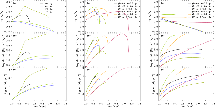
Figure 2.— Top row (a): Logarithm of the ratio between the sound crossing time $\tau_{s}$ and the accretion time scale $\tau_{a}$ against time for all models (from left to right: isothermal and turbulent, magnetic with constant pressure, and magnetic with varying external pressure, as indicated). For $\log\tau_{s}/\tau_{a}>0$, the assumption of hydrostatic equilibrium is invalid. Center row (b): Logarithm of the line mass accretion rates against time for all models, as above, used to highlight the effects of the filament evolution on the accretion rate. Bottom row (c): Logarithm of line mass against time for all models. Note that the critical line masses (eq. 2) depend on the effective sound speed, and are generally larger than the isothermal value.

3.1.2 Reference Radius $R_{ref}$

The reference radius $R_{ref}$ needed to calculate the steady-state, free-fall radial velocity profile (eq. 6) is a free parameter of the model. It has been set to $10$ pc for the current models (compared to $2$ pc in H13). Figure 3 (top panel) demonstrates the effect of the choice of $R_{ref}$ on $v_{R}$, for $R_{ref}=1,3,10$ pc. For realistic filament radii of $\sim 0.1$ pc, $v_{R}$ varies between $0.6$ and $0.85$ km s^-1, resulting in a variation in the accretion timescales of $30$%. These values are consistent with the accretion velocities derived by Kirk et al. (2013) for Serpens South.

Figure 3.— Accretion velocity $v_{R}$ (top, eq. 6) against radius, and corresponding over-density profile (bottom) for three reference radii $R_{ref}=1,3,10$ pc, assuming a line mass of $m=16.3$ M_⊙ pc^-1. The velocities stay below $1$ km s^-1, and the densities increase at most by a factor of $\lesssim 6$.

3.1.3 Isothermality

The assumption of isothermality enters in two places. (1) The filament profiles are derived for hydrostatic, infinite, isothermal cylinders (Ostriker, 1964). Arzoumanian et al. (2011) find radial temperature variations strong enough to susceptibly flatten the radial density profiles of corresponding hydrostatic cylinders, while Fischera & Martin (2012b) rely on dust temperatures derived at longer wavelengths, where temperature variations are less pronounced. Here, I follow the latter authors in assuming a constant temperature, mainly for the purpose to restrict the number of free parameters in the model. A more accurate treatment, also more consistent with observational evidence, will be discussed elsewhere.

(2) Taken at face value, the accretion velocities derived from the integration of eq. 5 would lead to shocks at Mach numbers of $10$ or more in some cases, or of shock velocities of up to a few km s^-1 in extreme cases (Fig. 1). Figure 3 (top panel) shows that the steady-state, free-fall velocity profile (eq. 6) expected for a line mass of $m=16.3$ M_⊙ pc^-1 is generally less than $1$ km s^-1, even for exceedingly large reference radii $R_{ref}$. Assuming $T=10$K, these $v_{R}$ correspond to Mach numbers of up to $5$. It also should be noted that $v_{R}\propto\sqrt{m}$, thus higher line masses do not affect $v_{R}$ strongly. Draine et al. (1983) give peak temperatures of a few hundred Kelvin for shocks in dense molecular gas ($n=10^{4}$ cm^-3) at a shock velocity of $5$ km s^-1, and with a radiative shock width of a $10^{-3}\cdots 10^{-2}$ pc. Due to the high densities (and thus, the high cooling rates), the shocks can be treated as isothermal beyond this length scale, thus justifying the isothermal assumption even for the most strongly accreting filaments in our models. The very assumption of an accretion shock may be unrealistic specifically in the cases with extreme $v_{R}$, since those correspond to models including accretion-driven turbulence. The turbulence itself implies that a well-defined filament boundary does not exist.

3.1.4 Background Density

The choice of the background density $n_{ext}$ plays a crucial role for the timescales discussed in §3.1.1: the accretion timescale depends linearly on $n_{ext}$ (see eq. 5), and our choice of $n_{ext}=P_{ext}/(\mu m_{H}c_{s}^{2})=2\times 10^{3}$ cm^-3 seems rather high for a molecular cloud envelope. Choosing a lower $n_{ext}$ by assuming a higher ambient temperature will extend the timescales by the same factor, thus bringing the isothermal case with constant pressure (”iso p₀”) into the regime $\tau_{s}/\tau_{a}<1$.

The background density $n_{ext}$ is assumed to stay constant over the evolution of the filament. This simplification serves mainly for consistency with previous models (H13), and it is also motivated to some extent by the column density profile shown in Figure 4 of Arzoumanian et al. (2011). Under more general conditions, the background density may change both in space (even at $t=0$) and with time, while the filament is accreting. Since it generally will drop, the evolution timescales derived here are lower limits. Figure 3 (bottom) shows the expected free-fall, steady-state density profile corresponding to the accretion velocities (top panel). The density profiles were found by integrating the continuity equation using eq. 6, and assuming a non-zero inward velocity component $v_{0}=c_{s}$ at $R_{ref}$. For plotting purposes, I set $n_{ext}=1$ cm^-3 in Fig. 3, yet, since a pressure-less accretion flow is assumed, this choice does not affect the density increase. In any case, the densities vary by a factor $\lesssim 6$ at most (for $m=16.3$ M_⊙ pc^-1).

3.1.5 Mass Reservoir

The center and bottom row of Figure 2 highlight the mass history of an accreting filament. The center row shows the mass accretion rates for all models, and the bottom row the actual line masses. Note that the critical line mass changes depending on the model assumptions, since the effective sound speed $\sigma$ may replace the actual sound speed $c_{s}$. Thus, all line masses shown in Figure 2 are subcritical with respect to $\sigma$, but may be supercritical with respect to $c_{s}$.

Kirk et al. (2013) estimate a lower limit for the radial accretion rate on Serpens South (with a line mass of $\sim 60$ M_⊙ pc^-1) of $130$ M_⊙ Myr^-1, corresponding to a line mass accretion rate of $390$ M_⊙ pc^-1 Myr^-1 at a filament length of $0.33$ pc.

Yet, some of the model accretion rates are substantial (e.g., model ”trb p₀”, and most of the magnetized models), to the point of being unrealistically high. For realistic background densities, the volume (strictly speaking, the cross section area) from which the filament would have to draw mass would extend out to a ”radius of influence”,

$$R_{i}=\sqrt{\frac{m}{\pi\rho}},$$ (17)

of several parsecs for $\dot{m}>100$ M_⊙ pc^-1 Myr^-1. Given the spatial scales and the background column densities seen in observations, this seems unrealistic. These high accretion rates are mostly a consequence of the filament’s expansion. The filaments expand most for models with constant external pressures, i.e. for cases where the infalling gas does not exert a corresponding ram pressure. In other words, the unrealistic results for these cases are a consequence of an inconsistency in the model setup – if we assume infall at multiples of the sound speed and non-negliglible densities, this mass flow should be dynamically important and ”squeeze” the filament, reducing the filament radius, and, hence, lowering the mass accretion rate.

3.1.6 Steady-State Accretion

The models rest on the assumption of steady-state, free-fall mass accretion (eq. 6), where the velocity profile $v_{R}$ evolves with the line mass, and thus with time. Any information about a change in the line mass travels over the ”radius of influence” (eq. 17) on time scales much shorter than the flow time scales. While inconsistent with the free-fall assumption (since the flow time scale is the same as the crossing time scale), it serves as a necessary simplification short of solving the fully time-dependent, hydrodynamical problem. This inconsistency will lead to an over-estimate of the mass accretion, and thus render evolutionary timescales as lower limits.

Starting with a fully-developed accretion profile at $t=0$, instead of gas at rest, may seem unrealistic, yet it is motivated by the need to actually form a seed filament by e.g. shock compression (Klessen et al., 2000; Padoan et al., 2001), possibly including thermal and shear effects (Hennebelle, 2013). Such a scenario of filament formation would require inflows, most likely at magnitudes higher than the assumed initial inflow velocities, which range around the value of the isothermal sound speed (Fig. 1).

Given that the ambient medium is pressurized, free-fall can only be assumed for $v(R_{f})\gg c_{s}$. This stage is reached for most models at $f>0.3$. Though this assumption is questionable for earlier stages, the choice of $f$ (as discussed in H13) just sets the initial mass of the filament, and thus depends somewhat on the filament formation scenario. In other words, assuming an instantaneous formation of a free-fall profile (see preceding discussion) allows us to neglect the flow history, and thus choose any value of $0<f<1$ as starting point.

Finally, given the initial conditions of a low-mass filament as “seed”, and with mass in the ambient medium than in the filament, one might argue whether the flows onto the filament would be more appropriately described as “global collapse” rather than “accretion”. I use the term “accretion” here to emphasize a connection to observed filaments, which are usually seen at an evolved stage.

3.2. Filament Evolution and FWHM($N_{c}$)-Correlations

In their Herschel study of dust filaments in Aquila, Polaris and IC5145, Arzoumanian et al. (2011) point out that the filament width does not depend on the central column density $N_{c}$, even for the thermally gravitationally unstable filaments in their sample (i.e. $f>1$ for $T=10$K. These will be referred to as ”nominally unstable”). They argue that a turbulent filament formation mechanism as discussed by Padoan et al. (2001) may explain the similar widths for nominally stable filaments (i.e. $f<1$), and that for nominally unstable ($f>1$) filaments it could be a consequence of continuing accretion, assuming a virialized filament.

H13 explored the role of turbulence on the filament accretion and subsequent evolution, finding that accretion-driven turbulence can in principle lead to a decorrelation of $N_{c}$ and FWHM, as speculated by Arzoumanian et al. (2011). To test whether the models discussed in this study are consistent with the previous results (and with observations), $500$ filament accretion models were run for each case considered (see Table 1).

Table 1Parameter ranges are indicated by $\dots$. For non-constant values, the relevant equation numbers are given.

model	$T_{0}$	$\sigma$	$\epsilon$	$\beta_{0}$	$s$	$p_{ext}$
	[K]					[$10^{4}$ K cm${}^{-3}]$
iso p0	$5\dots 15$	$c_{s}$	–	–	–	$2$
iso pv	$5\dots 15$	$c_{s}$	–	–	–	eq. 11
trb p0	$10$	eq. 12	$5\times 10^{-3}\dots 10^{-1}$	–	–	$2$
trb pv	$10$	eq. 12	$5\times 10^{-3}\dots 10^{-1}$	–	–	eq. 11
m05 p0	$10$	eq. 13	–	$10^{-1}\dots 10^{2}$	$0.5$	$2$
m10 p0	$10$	eq. 13	–	$10^{-1}\dots 10^{2}$	$1.0$	$2$
m05 pv	$10$	eq. 13	–	$10^{-1}\dots 10^{2}$	$0.5$	eq. 11
m10 pv	$10$	eq. 13	–	$10^{-1}\dots 10^{2}$	$1.0$	eq. 11

Figure 4 summarizes the test results. Each panel shows the probability to find a filament at a given position in $(\mbox{FWHM},N_{c})$ space during its evolution. Evolutionary tracks follow the overall envelope shapes, and in some cases, they are visible because of the finite sampling. The eight panels correspond to the eight cases summarized in Table 1. I overplotted the FWHM($N_{c}$) values for selected filaments in IC 5146, drawn from Arzoumanian et al. (2011, their Table 1). Colors indicate whether the filament contains YSOs (red), pre-stellar cores (blue), cores (green), or nothing (black). Overall, only a few of the eight cases allow a wide enough range in FWsHM consistent with the observed decorrelation between FWHM and $N_{c}$. I show the atomic central column density, consistent with FM12b, and in difference to Arzoumanian et al. (2011). Latter authors use the molecular column density, though their mean atomic weight seems to be inconsistent with that choice (see footnote in FM12b).

The isothermal case (“iso p₀”) reproduces Figure 10 of FM12a for a temperature of $T=10$ K (red dashed line). This is expected, yet it serves here as a consistency check. The tracks follow the instability line for large $N_{c}$, but, by construction, only stable filaments are allowed. FM12a discuss the possibility of projection effects (or viewing angles) to shift the evolutionary tracks to higher column densities, and thus break the strong FWHM$(N_{c})$-correlation, although they demonstrate that in this case, the high-column density filaments all would be seen at rather extreme inclination angles. Other possibilities would involve a non-uniform column density along the backbone of the filament (i.e. cores), pushing the average along the filament to higher values, or filaments embedded in a background medium of non-zero column density (Sec. 4). Column densities and FWsHM derived by FM12b for a sample of four filaments are consistent with model ”iso p₀” (dark green symbols in Fig. 4). Note that two of their filaments have also been analyzed by Arzoumanian et al. (2011), and that they arrive at different parameters. This may be just due to the different analysis methods, as discussed by FM12b.

If the external pressure contains a ram-pressure component (case “iso p_V”) due to the varying accretion velocity (eq. 11), the filament gets “squeezed”, and all characteristic scales shrink. The FWsHM now mostly lie below the observed range. The overall distribution is flatter than for the isothermal case with constant pressure, suggesting that varying pressures can lead to a decorrelation between $N_{c}$ and the FWHM. Yet, since free-fall accretion has been assumed, the external ram pressure will be a generous upper limit, suggesting that for lower and more realistic ram pressure estimates, the distribution of filament trajectories could move towards higher FWsHM. This would also reduce the effect of the ram pressure over the external pressure, thus increasing the curvature of the trajectories again, and thus converging to the constant pressure case. Only if the external constant pressure component were reduced substantially (by a factor of $10$), the trajectories could be shifted into the observed FWHM range.

The turbulent case with constant external pressure (“trb p₀”) does not require much discussion: the unconstrained filament is rapidly expanding, even seemingly avoiding the observed parameter ranges (see also §3.1.5). Adding a ram pressure component again pressurizes the filament (“trb p_V”). The FWHM distribution is much narrower than for the isothermal case, because of the lower power with which the filament properties depend on the turbulent driving efficiency (eq. 12). The distribution extends into the nominally (isothermally) unstable regime and has flattened, yet, the values lie again below most of the observed parameters.

Introducing a magnetic field assuming mass and flux conservation (“$s=0.5$ p₀”) results in a trajectory distribution similar to that of the isothermal case, since the magnetic field for $s=0.5$ just contributes a constant addition to the sound speed (eq. 13). A decorrelation of $N_{c}$ and FWHM only would be expected if filaments at low and high central column densities are less magnetized than those at intermediate $N_{c}$ – a not entirely convincing scenario. The situation improves drastically when adding the ram pressure to the external pressure (“$s=0.5$ p_V”). The trajectories are now fairly flat, with the FWHM depending only weakly on $N_{c}$, and they are approximately within the observed range.

A poloidal or toroidal field (“$s=1.0$ p₀” and “$s=1.0$ p_V”) also leads to a decorrelation between FWHM and $N_{c}$, yet, due to the magnetization now increasing with the filament density, the filament scales increase well above the observed range. One could speculate whether such broad filaments could be missed in the observational analysis, since they essentially would appear as background. Yet note that these cases are equivalent to an effective equation of state with $\gamma=2$, since $B\propto n$.

From the above discussion, we conclude the following:

(a)

The isothermal case as discussed by FM12a is unlikely to show a decorrelation of FWHM and $N_{c}$ to the extent observed by Arzoumanian et al. (2011). Especially when approaching the instability line (dashed diagonals in Figure 4), the correlation becomes inevitable just by construction. The column densities and FWsHM derived by FM12b (their Fig. 7) for low-mass filaments are consistent with the isothermal case (dark green symbols, dashed red line).

(b)

The ram-pressurized, isothermal case, and the turbulent cases (while still assuming – in contrast to H13 – $p=4$) cannot break the correlation, unless unrealistically low external constant pressure components are assumed.

(c)

Magnetic fields scaling linearly with density (i.e. an effective $\gamma=2$) lead to a decorrelation, but also to filament widths substantially larger than observed.

(d)

The best agreement is found for magnetic fields scaling weakly with density, especially if the external pressure contains a ram pressure component. Since $s=1/2$ is equivalent with mass and flux conservation, this result is consistent with the filaments embedded in three-dimensional extended structures of more diffuse, magnetized material. Reasonably, one could assume this to be the most realistic case also. Heyer et al. (2008) found striations in the molecular gas to be aligned with magnetic field vectors inferred from polarimetry in Taurus, consistent with kinematic evidence. The same pattern has been observed in much greater detail in dust column density maps (Palmeirim et al., 2013). Such structures are consistent with a radial field component (in the plane of sky) around an accreting filament. From field geometry considerations, the field is probably not perfectly radial for all azimuthal directions around the filament. Yet, if the filament were embedded in a flattend cloud, the observed field directions would be also restricted to the plane of the cloud. This is the situation envisaged for the case $s=0.5$ discussed above.

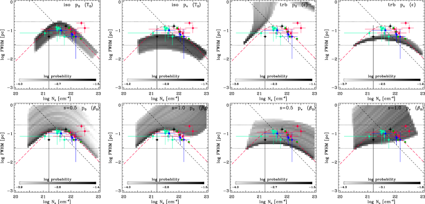
Figure 4.— Probability density map of FWHM against atomic column density for all cases considered in §2. The relevant physical parameters are indicated in each panel, including the parameter that is varied for each set of models (in parentheses), and the sampling ranges are given in Table 1. The plots can be directly compared to Figure 7 of Arzoumanian et al. (2011), or Figure 7 of FM12b. The range of observed FWsHM is given by the dotted lines, and the dashed line indicate the Jeans length, Observed filament values are plotted as diamonds, with colors indicating whether the filament contains YSOs (red), pre-stellar cores (blue), cores (light green), or nothing (black). Dark green diamonds indicate the values derived by FM12b.

4. Filaments within Sheets

Given the observed column density and magnetic field structures around molecular filaments, it is not unreasonable to assume that the filaments are embedded within structures of the next higher dimensions, i.e. within flattened clouds, or sheets. Pon et al. (2011) discuss a sequence of gravitational collapse, from higher to lower dimensions, consistent with filaments embedded in sheets. Flattened structures result also naturally from clouds forming in large-scale flows. In the following, I develop a simple model of a filament embedded in a sheet, with the goal to explain the flattening of observed filament profiles in comparison with the hydrostatic cylinder. This might be considered a logical extension of the discussion by FM12a: not only is it realistic to assume that the filament is embedded within a medium of non-zero pressure, but also of non-zero density. The latter effect will be discussed here, with the goal to develop an observational diagnostic identifying the evolutionary stage of the filament (parameterized by the criticality parameter $f$, eq. 3), and the projection angle between the line-of-sight and the embedding sheet (see Fig. 5).

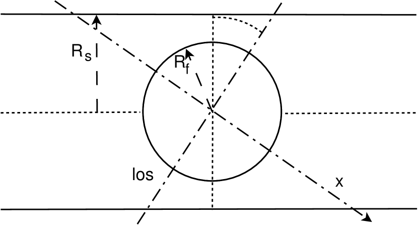
Figure 5.— Sketch of the geometry of a filament of radius $R_{f}$ embedded in a sheet of thickness $2R_{s}$ (case $R_{f}<R_{s}$ shown). The projection angle $\cos\beta$ is measured between the line of sight and the normal onto the filament and plane, as indicated.

4.0.1 Flattening of Profiles

Arzoumanian et al. (2011) conclude that their identified filaments have radial column density profiles generally flatter than those expected for an isothermal, infinite cylinder (see also Palmeirim et al., 2013). FM12a explain the flatness of the profiles with external pressurization: only for zero external pressure, the filament will show a density profile $\propto R^{-4}$ (see their Fig. 3). Here, I explore the effect of a non-vanishing background column density on the derived filament properties, specifically on the steepness of the profile, parameterized by the power law index $p$ (see eq. 1). A vanishing background density would be fully appropriate only if the temperature outside the filament is high enough to render the ambient density (and thus column density) below the observational sensitivity.

For the following analysis, I consider an externally pressurized filament of radius $R_{f}$ embedded in a sheet of thickness $2R_{s}$. Thus, if $R_{s}=R_{f}$, the filament fits snugly into the sheet. We are interested in the total column density profile $N_{tot}(x)$ through the filament and the ambient sheet, depending on the viewing angle $\cos\beta$, with $\cos\beta=1$ indicating a line-of-sight perpendicular to the sheet, and $\cos\beta=0$ parallel to the plane defined by the sheet, and perpendicular to the filament (see Fig. 5). For $\cos\beta=1$, $N_{tot}(0)=N_{c}$. The radius $x$ measures the distance in the plane-of-sky, normalized to the filament radius $R_{f}$. The column density of the filament $N_{f}(x)$ is given by eq. 15 of FM12a, where the constant external pressure $p_{ext,0}$ is replaced by equation 11. The column density of the ambient gas is

$$N_{s}(x) = 2n_{ext}\left(\frac{R_{s}}{\cos\beta}-R_{f}(1-\bar{x}^{2})^{1/2}\right),\mbox{ with}$$ (18)

$$\bar{x} \equiv \min(1,x).$$ (19)

Thus, we can express the total column density $N_{tot}=N_{f}(x)+N_{s}(x)$ for sheets of varying thickness, and viewed under arbitrary angles. Obviously, eq. 18 only holds if the embedding sheet extends at least a distance

$$D_{min}=\frac{R_{s}/R_{f}}{\tan(\pi/2-\beta)}$$ (20)

from the filament center.

The above equations allow us to generate a set of filament models in dependence of $f$ and $\cos\beta$. For each pair $(f,\cos\beta)$, a column density profile results that is fit with the profile given by Arzoumanian et al. (2011, their eq. 1), resulting in a flatness parameter $p$, a core radius $R_{0}$ (their $R_{flat}$), and the ratio of the column density over the background column

$$Q_{N}\equiv N_{tot}(0)/N_{s}(R_{f}).$$ (21)

The fit parameters have errors less than $3$% for $f<0.99$ and $\cos\beta>10^{-2}$, i.e. they are useful for reasonable ranges of $f$ and $\cos\beta$.

If the exponent $p$ and the column density ratio $Q_{N}$ are known from observations, then the projection angle $\cos\beta$ and the criticality parameter $f$ of the pressurized filament can be estimated by minimizing

$$\Delta^{2}_{f,\beta}\equiv\left(\left(\frac{Q_{N}(obs)-Q_{N}(f,\cos\beta)}{Q_{N}(f,\cos\beta)}\right)^{2}+\left(\frac{p(obs)-p(f,\cos\beta)}{p(f,\cos\beta)}\right)^{2}\right)$$ (22)

over a map of $(f,\cos\beta)$. The subscript $obs$ indicates the observed values. The top row of Figure 6 indicates how reliable such estimates might be. It shows contour lines of $p$ (solid lines) and $Q_{N}$ (dashed line), in the $(f,\cos\beta)$-plane, for three values of $R_{s}/R_{f}=1,1.5,2$. The contours are labeled with their respective values. The central column density depends on $f$ through eq. 15 of FM12a, while the total column through filament and sheet depends on the angle $\cos\beta$ via eq. 18. The black symbols plotted over the contour lines are used as a check how reliably eq. 22 can retrieve the parameters. A $100$ randomly chosen points, uniformly distributed in $\cos\beta$ and $f$, were used to calculate the corresponding $Q_{N}$ and $p$ values. For the physically interesting ranges of $f$ and $\cos\beta$ as mentioned above, the values are recovered with less than $3$% error, not surprisingly consistent with the fit accuracies.

The method works best for thin sheets – since the sheet column density does not depend on $f$, angles between contours of $p$ and $Q_{N}$ are larger for larger $f$, and thus degeneracies between $f$ and $\cos\beta$ are less likely to occur. With increasing $R_{s}/R_{f}$, the curves start to align, and thus the estimates of $\cos\beta$ and $p$ will be correspondingly less certain.

Taking the column density values and $p$ values from Table 1 of Arzoumanian et al. (2011) and applying equation 22 generates the red symbols in Figure 6. We note the following issues: (a) With increasing $R_{s}$ (center and right panel), the observed points move towards $\cos\beta=1$. This is just because for increasing sheet thickness, the contrast $Q_{N}$ drops. While we cannot determine $R_{s}$ independently, one could argue from the distribution in $\cos\beta$ that larger $R_{s}$ values may be unrealistic, since they would entail $\cos\beta=1$ for most filaments. (b) Most of the observed points cluster at $0.9<f<1$ and small $\cos\beta$. Taken at face value, this would mean that for most of the filaments, the line-of-sight is nearly parallel to the embedding sheet. This may (or may not) be an unsatifactory conclusion, and could be tested with kinematic data. Yet, it should be pointed out that all those points correspond to fairly high $Q_{N}$ and low $p$, a region of the parameter space where the curves of constant $N$ and $p$ are nearly parallel. Also, the models used to generate the $(p,Q_{N})$-curves assume that the actual density profile corresponds to an isothermal cylinder, with $p=4$ in vacuum.

The clustering of the observed value in a nearly inaccessible parameter region suggests to check the underlying distribution of $(p,Q_{N})$-values for the observations (red symbols in Figure 6, bottom) and test models (black symbols). The difference between both distributions is obvious: randomly choosing values in $\cos\beta$ and $f$ does not lead to a full coverage of $(p,Q_{N})$-space, as already evident from the contour distribution in Figure 6. Yet, these are the values that are “allowed” in this simple model, assuming a hydrostatic cylinder embedded in a sheet. While the modeled values can reach high $Q_{N}$ only for large $p$, the observed values are clustered at lower $p$, with similarly high $Q_{N}$ values. Only the low-$Q_{N}$ regime shows overlap. Increasing $R_{s}$ closes the gap between the two distributions somewhat, yet, it also reduces the $Q_{N}$ values modeled. If the modeled $Q_{N}$ are to be kept at similar levels, larger $f$ are required.

Summarizing, the observed regime of high $Q_{N}$ and low $p$ is not accessible by an isothermal, externally pressurized cylinder embedded in a sheet. Low $p$ would entail a small $\cos\beta$ in the model (and a small $Q_{N}$), since the profiles flatten with decreasing $\cos\beta$ and $f$. To drive up the contrast to observed values, a correspondingly larger value of $f$ would have to be chosen. The reason for the failure lies in the fact that the intrinsic (3D) profile still has $p=4$, and the flattening is solely due to a lower $f$ (and thus larger $R_{0}$) and/or a lower $\cos\beta$ or higher background column density. Thus, low $p$ is interpreted as a low $f$ and hence a low $Q_{N}$, whereas a low $p$ and high $Q_{N}$ would require extremely small $\cos\beta$ or high backgrounds to “hide” the over-density.

While the described method to estimate the evolutionary stage of a filament and its environment fails for the isothermal cylinder, the technique might prove useful for more generalized cylinder models, specifically for models with flatter intrinsic profiles.

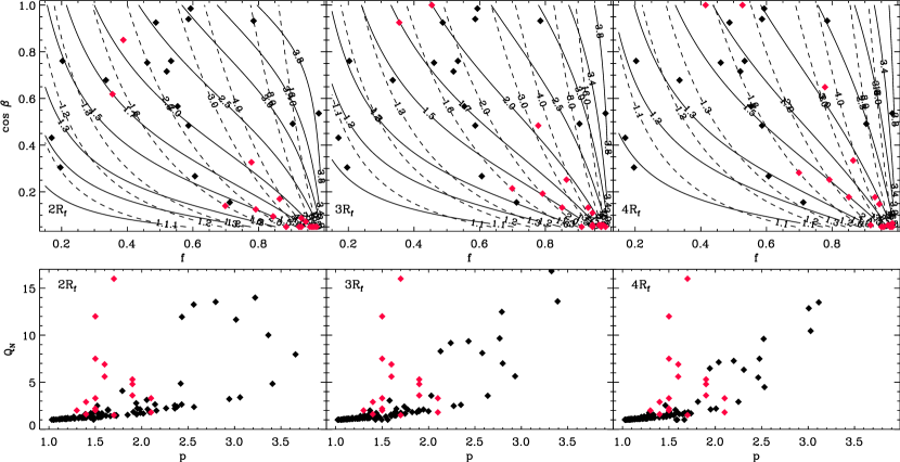
Figure 6.— Top: Contour lines of the profile exponent $p$ (solid lines) and the central to background column density $Q_{N}$ (eq. 21, dashed lines) in terms of the criticality parameter $f$ and the viewing angle $\cos\beta$ (see text). If $p$ and $N_{c}/N_{ext}$ can be determined from observations, the three diagrams provide estimates for the evolutionary stage of the filament in terms of $f$, and the viewing angle $\cos\beta$, for a filament as modeled above embedded in a sheet of thickness $2,3$, and $4R_{f}$ (left to right, indicated in bottom left of each panel). All three diagrams use the same set of contour levels. For $p$, these are given by $p=[1.1,1.2,1.3,1.7,2.0,2.5,3.0,3.4,3.8]$, and $N_{c}/N_{ext}=[1.1,1.2,1.3,1.6,2.0,3.0,4.0,8.0,16.0]$. For increasing embedding sheet thickness, the contours shift to higher $f$. Bottom: Distribution of observed filaments (red symbols; taken from Table 1 of Arzoumanian et al. 2011)

4.0.2 Temperature Profiles

Here, we briefly speculate on the effect of different temperatures in the filament and the embedding sheet on the overall temperature profile of an observed filament in dependence of the viewing angle $\cos\beta$. Two constant temperatures for the sheet, $T_{s}=15$ K, and for the filament, $T_{f}=10$ K, are assumed. The temperature profile is then integrated along the line-of-sight set by $\cos\beta$ as

$$T(x)=\frac{N_{f}(x)T_{f}+N_{s}(x)T_{s}}{N_{tot}(x)},$$ (23)

with the projected distance to the filament center $x$, measured in units of $R_{f}$.

The results for the three values of $R_{s}=1.0,1.5,2.0$ are summarized in Figure 7. Already this simple temperature distribution and geometry can generate temperature profiles consistent with observations. Note that this is not intended to suggest that observed filaments are isothermal. The only point being made here is to show that projection effects can have a substantial effect on the derived temperature, of the same order as intrinsic temperature variations.

Figure 7.— Column density (top) and temperature (bottom) profiles of a pressurized, hydrostatic, isothermal cylinder at $f=0.8$, embedded in a sheet of uniform density $n_{ext}$ and thickness of $2,3$, and $4R_{f}$ (left to right, as indicated in panels). Temperatures in the sheet and filament are assumed to be constant, at $T_{s}=15$ K and $T_{f}=10$ K, respectively. Assuming density-weighted temperatures, already this simple geometry can lead to temperature profiles consistent with observations.

5. Conclusions

In an extension of Fischera & Martin (2012a) and Heitsch (2013), the evolution of a pressurized, hydrostatic cylinder accreting gas at free-fall velocities is studied. FM12a discussed the problem of an externally pressurized, isothermal cylinder, and how such a model would explain Herschel observations of molecular cloud filaments and their stability (FM12b). H13 explored the effect of accretion on a filament described by a central density, a core radius, and a power-law profile with exponent $p$, following the parameterization by Arzoumanian et al. (2011).

Here, the goal is to merge the two models. The main difference to FM12a is that the external pressure is allowed to vary due to the ram pressure exerted by the infalling gas (eq. 11). This additional pressurization leads to a compression of the filament. Unlike H13 (and following FM12a), a physical model for the filament is assumed, namely a hydrostatic isothermal cylinder, thus motivating the choice of $p$.

The accretion models (Fig. 1) reproduce the results by FM12a for the isothermal case. Ram-pressurized, hydrodynamical accretion models lead to filament FWsHM an order of magnitude smaller than observed (Fig. 4), suggesting that (a) the ram pressure is being over-estimated, due to the strong free-fall assumption (see discussion by H13) or (b), that – since H13 could explain the decorrelation between FWHM and $N_{c}$ for filaments flatter than isothermal – the isothermal cylinder is not a fully adequate description for currently observed filaments. Yet, FM12b demonstrate that for their sample of low-filaments (two of which are re-analyzes of filaments discussed by Arzoumanian et al. (2011)), the isothermal cylinder provides a good description for the observed $N(FWHM)$ values. These differences in the interpretation of observational data may well still be due to the specific analysis techniques and selection of filament (sections) used by each of these authors

While magnetized accretion models other than the simplest, magnetosonic case can reproduce a decorrelation, cases with strong magnetic scaling $B\propto n$ result in a FWHM distribution substantially broader than observed. Only the ram-pressurized weak scaling case shows some promise to reproduce observed FWHM$(N_{c})$ values adequately. This seems a reasonable conclusion in face of observed column density striations aligned with magnetic field vectors around Taurus molecular filaments (Heyer et al., 2008; Palmeirim et al., 2013), if a filament-in-sheet geometry is assumed.

This filament-in-sheet geometry is explored to some extent in §4. Extending FM12a’s reasoning and assuming not only a non-zero ambient pressure, but also a non-zero ambient density, suggests that in the simplest case, a pressurized filament would sit in a sheet of some thickness equal to or larger than the filament diameter (Fig. 5). Such a configuration would lead to a natural flattening of the profile, in addition to a flattening introduced by reducing the evolution parameter $f$. Given observed profile parameters $p$ and column density contrasts $Q_{N}$ (eq. 21) between central and ambient column density, the viewing angle $\cos\beta$ and the evolution parameter $f$ can be estimated (Fig. 6). Testing this method with the data from Arzoumanian et al. (2011) demonstrates that the observed parameter regime of high $Q_{N}$ and low $p$ is not accessible by a simple filament-in-sheet geometry, for any kind of ratio $R_{s}/R_{f}$, if the cylinder is isothermal.

Appendix A Summary of Fischera & Martin (2012a)

The relevant expressions of Fischera & Martin (2012a, see their section 2) are briefly summarized. The density profile of an isothermal, hydrostatic, infinite cylinder is given by

$$\rho(R)=\rho_{c}\left(1+\left(\frac{R}{R_{0}}\right)^{2}\right)^{-2}$$ (A1)

(Ostriker, 1964), with the core radius $R_{0}$ given by equation 4. The corresponding line mass in dependence of the filament radius is

$$f(R_{f})=\frac{m}{m_{cr}}=1-\frac{1}{1+R_{f}^{2}/R_{0}^{2}},$$ (A2)

and thus, with $p(R_{f})=\rho(R_{f})c_{s}^{2}=p_{ext}$, the central density in terms of the external pressure is given by

$$\rho_{c}=\frac{p_{ext}}{c_{s}^{2}}(1+R_{f}^{2}/R_{0}^{2})=\frac{p_{ext}}{c_{s}^{2}}\frac{1}{(1-f)^{2}}.$$ (A3)

Using equations 4 and A2 results in the filament radius

$$R_{f}=c_{s}^{2}\left(\frac{2f(1-f)}{\pi Gp_{ext}}\right)^{1/2}.$$ (A4)

As Fischera & Martin (2012a) show in their Figure 3, the overpressure $p_{c}/p_{ext}$ will determine the steepness of the resulting density profile: for large over-pressures (or $R_{f}/R_{0}\gg 1$), the profiles approach the vacuum solution $\propto R^{-4}$. Thus, the overpressure will determine the ”flatness” of the cylinder profile.

Appendix B Pressurized Filaments: Expressions for Root Finders

I summarize the expressions and methods to derive the filament accretion rate, assuming an externally pressurized, hydrostatic filament. To integrate the line mass density (eq. 5), the filament radius $R_{f}$ (eq. 7), the criticality parameter $f$ (eq. 3), and the sound speed $\sigma$ are needed in the RHS of the ODE. For most of the cases, $R_{f}$ depends on itself in a non-trivial way, through the ram pressure or through the sound speed. The approaches to resolve these dependencies are discussed in the following. The full expressions and their implementation can be found at www.physics.unc.edu/$\sim$fheitsch/codesdata.php

B.1. Constant $\sigma$, varying external pressure

This is the case ”iso p${}_{\mbox{v}}$” in Figure 1. The external pressure in eq. 7 is replaced by the combination of ram pressure and constant thermal pressure, eq. 10, resulting in

$$1-\frac{\sigma^{2}}{R_{f}}\left(\frac{2f(1-f)}{\pi G(p_{ext,0}+4Gmq\rho_{ext})}\right)^{1/2}\equiv 0,$$ (B1)

where

$$q\equiv\ln\frac{R_{ref}}{R_{f}}.$$ (B2)

Equation B1 can be solved with a simple root finder.

B.2. Accretion-driven turbulence, constant external pressure

This is the case “trb p₀” in Figure 1. The soundspeed $\sigma=c_{s}$ is replaced by equation 12. It turns out to be advantageous in terms of accuracy and convergence speed to solve the dependencies with a Newton-Raphson method for the scaled filament radius $\bar{R}\equiv R_{f}/R_{pc}$, where $R_{pc}$ is a scaling number. Thus, we get the following expression:

$$y(R) = \frac{\sigma^{2}}{\bar{R}R_{pc}}\left(\frac{2f(1-f)}{\pi Gp_{ext,0}}\right)^{1/2}-1$$

$$= uvw-1\equiv 0$$

with

$$u = \frac{1}{\bar{R}R_{pc}}$$ (B4)

$$v = \sigma^{2}$$ (B5)

$$w = \left(\frac{2f(1-f)}{\pi Gp_{ext,0}}\right)^{1/2}.$$ (B6)

The Newton-Raphson root finder also requires the derivative with respect to $\bar{R}$,

$$y^{\prime}=u^{\prime}\,v\,w+u\,v^{\prime}\,w+u\,v\,w^{\prime},$$ (B7)

with the derivatives

$$u^{\prime} = -\frac{u}{\bar{R}}$$ (B8)

$$v^{\prime} = 2\sigma\sigma^{\prime}=a_{2}\bar{R}^{1/3}\left(\frac{4}{3}q-1\right),$$ (B9)

$$w^{\prime} = \frac{1-2f}{(2\pi Gp_{ext,0}f(1-f))^{1/2}}\,f^{\prime},$$ (B10)

$$f^{\prime} = -\frac{a_{2}mG\bar{R}^{1/3}}{2\sigma^{4}}\left(\frac{4}{3}q-1\right).$$ (B11)

Here, $a_{2}$ is a constant of the value

$$a_{2}\equiv 4\left(4\pi\epsilon(G^{3}m)^{1/2}\rho_{ext}R_{pc}^{2}\right)^{2/3}.$$ (B12)

B.3. Accretion-driven turbulence, varying external pressure

This is the case “trb p_V” in Figure 1. The soundspeed $\sigma=c_{s}$ is replaced by equation 12 again, and the external pressure is given by equation 11. As in the previous case (§B.2), we use a Newton-Raphson method for the scaled filament radius $\bar{R}\equiv R_{f}/R_{pc}$. The expressions for $u$ and $v$ are identical to those in equations B4 and B5, since they do not depend on the external pressure. For $w$ we now get

$$w=\left(\frac{2f(1-f)}{\pi Gp_{ext}}\right)^{1/2},$$ (B13)

and

$$w^{\prime} = \left(\frac{1}{2\pi G}\right)^{1/2}\frac{p_{ext}(1-2f)f^{\prime}-f(1-f)p^{\prime}_{ext}}{wp_{ext}^{2}},$$ (B14)

$$p^{\prime}_{ext} = -4Gm\frac{\rho_{ext}}{\bar{R}}.$$ (B15)

B.4. Accretion of magnetic fields, constant external pressure

The magnetic case with constant external pressure requires replacing the sound speed by equation 13. The expressions are simple enough that we can treat both $s=1/2$ and $s=1$ in one branch (this will change in the next step), thus we get the following expression for the root function (it is numerically more advantageous to solve for $\sigma$ instead of $R_{f}$) and its derivative:

$$y(\sigma)=\frac{\sigma}{c_{s}}-u$$ (B16)

$$y^{\prime}=\frac{1}{c_{s}}-\frac{a_{4}mG(2s-1)w^{-4s+1}}{u^{1/2}\sigma^{3}},$$ (B17)

with the auxilliary functions

$$u = \left(1+a_{4}w^{-2(2s-1)}\right)^{1/2}$$ (B18)

$$w = 1-f=1-\frac{mG}{2\sigma^{2}}.$$ (B19)

The constant $a_{4}$ is given by

$$a_{4}=\frac{2}{\beta_{0}}\left(\frac{p_{ext,0}}{\rho_{c0}c_{s}^{2}}\right)^{2s-1}.$$ (B20)

B.5. Accretion of magnetic fields, varying external pressure, $s=1/2$

In this case, the effective sound speed (eq. 13) simplifies to $\sigma^{2}=c_{s}^{2}(1+2/\beta_{0})$. We use a Newton-Raphson method to find the root for the (scaled) radius equation,

$$y(\bar{R})=1-\frac{a_{5}}{\bar{R}}\,(2b_{5}\,q+p_{ext,0}),$$ (B21)

with the constants

$$a_{5} = \frac{\sigma^{2}}{R_{pc}}\left(\frac{2f(1-f)}{\pi G}\right)^{1/2}$$ (B22)

$$b_{5} = 4\pi G\rho_{ext}m.$$ (B23)

The derivative with respect to $\bar{R}$ is given by

$$y^{\prime}=\frac{a_{5}}{\bar{R}^{2}}\frac{2(b_{5}q+p_{ext,0})+b_{5}}{2(b_{5}q+p_{ext,0})^{3/2}}.$$ (B24)

B.6. Accretion of magnetic fields, varying external pressure, $s=1$

Replacing the central density in equation 13 by equation A3, the effective soundspeed is now given by

$$\sigma=c_{s}\left(1+\frac{2}{\beta_{0}}\frac{p_{ext}}{p_{ext,0}(1-f)^{2}}\right)^{1/2},$$ (B25)

where $p_{ext}$ is defined by equation 11. Equation B25 results in a cubic for $\sigma^{2}$, with the solution

$$\sigma^{2} = \frac{2^{1/3}a_{6}^{2}}{3D^{1/3}}+\frac{D^{1/3}}{32^{1/3}}-\frac{2^{1/3}b_{6}}{D^{1/3}}+\frac{a_{6}}{3}$$ (B26)

$$D = 2a_{6}^{3}+\sqrt{27}\sqrt{4a_{6}^{3}c_{6}-a_{6}^{2}b_{6}^{2}-18a_{6}b_{6}c_{6}+4b_{6}^{3}+27c_{6}^{2}}-9a_{6}b_{6}+27c_{6}$$ (B27)

$$a_{6} = \frac{mG}{2}+c_{s}^{2}\left(1+\frac{2}{\beta_{0}}\frac{p_{ext}}{p_{ext,0}}\right)$$ (B28)

$$b_{6} = mG(mG/4+c_{s}^{2})$$ (B29)

$$c_{6} = (mGc_{s})^{2}/4.$$ (B30)

With $\sigma$ in hand, we can write the root function for the scaled radius,

$$y(\bar{R}) = uvw-1$$ (B31)

$$u = \frac{1}{\bar{R}R_{pc}}$$ (B32)

$$v = \sigma^{2}$$ (B33)

$$w = \left(\frac{2f(1-f)}{\pi Gp_{ext}}\right)^{1/2}.$$ (B34)

The derivative is formally given by equation B7. If we label the four terms of $\sigma^{2}$ in equation B26 as $S_{1},S_{2},S_{3},S_{4}$, the derivative of $\sigma$ is

$$\sigma^{\prime} = \frac{1}{2\sigma}(S^{\prime}_{1}+S^{\prime}_{2}+S^{\prime}_{3}+S^{\prime}_{4})$$ (B35)

$$S^{\prime}_{1} = \frac{2^{1/3}a_{6}}{3D^{1/3}}\left(2a^{\prime}_{6}-\frac{aD^{\prime}}{3D}\right)$$ (B36)

$$S^{\prime}_{2} = \frac{1}{9\cdot 2^{1/3}}D^{-2/3}D^{\prime}$$ (B37)

$$S^{\prime}_{3} = -\frac{2^{1/3}b_{6}}{3}D^{-4/3}D^{\prime}$$ (B38)

$$S^{\prime}_{4} = \frac{1}{3}a^{\prime}_{6}$$ (B39)

$$D^{\prime} = \left(6a_{6}^{2}+\frac{3}{2}\frac{\sqrt{3}(12a_{6}^{2}c_{6}-2a_{6}b_{6}^{2}-18b_{6}c_{6}}{\sqrt{4a_{6}^{3}c_{6}-a_{6}^{2}b_{6}^{2}-18a_{6}b_{6}c_{6}+4b_{6}^{3}+27c_{6}^{2}}}-9b_{6}\right)a^{\prime}_{6}$$ (B40)

$$a^{\prime}_{6} = -8\frac{\rho_{ext}mGc_{s}^{2}}{\beta_{0}p_{ext,0}\bar{R}}.$$ (B41)

The derivative of $w$ is given by equation B14, with $f^{\prime}$ replaced by

$$f^{\prime}=-\frac{2f}{\sigma}\sigma^{\prime}.$$ (B42)

References

- Arzoumanian et al. (2011) Arzoumanian, D., André, P., Didelon, P., 2011, et al. A&A, 529, L6
- Draine et al. (1983) Draine, B. T., Roberge, W. G., & Dalgarno, A. 1983, ApJ, 264, 485
- Fiege & Pudritz (2000a) Fiege, J. D. & Pudritz, R. E. 2000a, MNRAS, 311, 85
- Fiege & Pudritz (2000b) —. 2000b, MNRAS, 311, 105
- Field et al. (2008) Field, G. B., Blackman, E. G., & Keto, E. R. 2008, MNRAS, 385, 181