Approximating spectral densities of large matrices

Abstract

In physics, it is sometimes desirable to compute the so-called Density Of States (DOS), also known as the spectral density, of a real symmetric matrix $A$. The spectral density can be viewed as a probability density distribution that measures the likelihood of finding eigenvalues near some point on the real line. The most straightforward way to obtain this density is to compute all eigenvalues of $A$. But this approach is generally costly and wasteful, especially for matrices of large dimension. There exists alternative methods that allow us to estimate the spectral density function at much lower cost. The major computational cost of these methods is in multiplying $A$ with a number of vectors, which makes them appealing for large-scale problems where products of the matrix $A$ with arbitrary vectors are relatively inexpensive. This paper defines the problem of estimating the spectral density carefully, and discusses how to measure the accuracy of an approximate spectral density. It then surveys a few known methods for estimating the spectral density, and proposes some new variations of existing methods. All methods are discussed from a numerical linear algebra point of view.

1 Introduction

Given an $n\times n$ real symmetric and sparse matrix $A$, scientists in various disciplines often want to compute its Density Of States (DOS), or spectral density. Formally, the DOS is defined as

$$\phi(t)=\frac{1}{n}\sum_{j=1}^{n}\delta(t-\lambda_{j}),$$ (1)

where $\delta$ is the Dirac distribution commonly referred to as the Dirac $\delta$-“function” [37, 4, 35], and the $\lambda_{j}$’s are the eigenvalues of $A$, assumed here to be labeled non-decreasingly. Using the DOS, the number of eigenvalues in an interval $[a,b]$ can be formally expressed as

$$\nu_{[a,b]}=\int_{a}^{b}\sum_{j}\delta(t-\lambda_{j})\ dt\equiv\int_{a}^{b}n\phi(t)dt.$$ (2)

Therefore, one can view $\phi(t)$ as a probability distribution “function”, which gives the probability of finding eigenvalues of $A$ in a given infinitesimal interval near $t$. If one had access to all the eigenvalues of $A$, the task of computing the DOS would become a trivial one. However, in many applications, the dimension of $A$ is large. The computation of its entire spectrum is prohibitively expensive, and this leads to the need to develop efficient alternative methods to estimate $\phi(t)$ without computing eigenvalues of $A$. Since $\phi(t)$ is not a proper function, we need to clarify what we mean by “estimating” $\phi(t)$, and this will be addressed in detail shortly. For now we can use our intuition to argue that $\phi(t)$ can be approximated by dividing the interval containing the spectrum of $A$ into many sub-intervals and use a tool like Sylvester’s law of inertia to count the number of eigenvalues within each of these sub-intervals. This approach yields a histogram of the eigenvalues. Expression (2) will then provide us with an average “value” of $\phi(t)$ in each small subinterval $[a,b]$. As the size of each subinterval decreases, the histogram approaches the spectral density of $A$. However, this is not a practical approach since performing such an inertia count requires us to compute the $LDL^{T}$ factorization [18] of $A-t_{i}I$, where the $t_{i}$’s are the end points of the subintervals. In general, this approach is prohibitively expensive because of the large number of intervals needed and the shear cost of each factorization. Therefore, a procedure that relies entirely on multiplications of $A$ with vectors is the only viable approach.

Because calculating the spectral density is such an important problem in quantum mechanics, there is an abundant literature devoted to this problem and research in this area was extremely active in the 1970s and 1980s, leading to clever and powerful methods developed by physicists and chemists [12, 42, 10, 44] for this purpose.

In this survey paper, we review two classes of methods for approximating the spectral density of a real symmetric matrix from a numerical linear algebra perspective. For simplicity, all methods are presented using real arithmetic operations, i.e. we assume the matrix is real symmetric. The generalization to Hermitian matrices is straightforward. The first class of methods contains the Kernel Polynomial Method (KPM) [39, 43] and its variants. The KPM can be viewed as a formal polynomial expansion of the spectral density. It uses a moment matching method to derive the coefficients for the polynomials. The method, which is widely used in a variety of calculations that require the DOS [13], has continued to receive a tremendous amount of interest in the last few years [13, 6, 25, 38]. We show that a less well known, but rather original, method due to Lanczos and known as the “Lanczos spectroscopic” procedure, which samples the cosine transform of the spectral density, is closely related to KPM. As another variant of KPM, we present a spectral density probing method called Delta-Gauss-Legendre method, that can be viewed as a polynomial expansion of a smoothed spectral density. The second class of methods we consider uses the classical Lanczos procedure to partially diagonalize $A$. The eigenvalues and eigenvectors of tridiagonal matrix are used to construct approximations to the spectral density.

One of the key ingredients used in most of these methods is a well-established artifice for estimating the trace of a matrix. For example, the expansion coefficients in the above-mentioned KPM method can be obtained from the traces of the matrix polynomials $T_{k}(A)$, where $T_{k}$ is the Chebyshev polynomial of degree $k$. Each of these is in turn estimated as the mean of $v^{T}T_{k}(A)v$ over a number of random vectors $v$. This procedure for estimating the trace has been discovered more or less independently by statisticians [21] and physicists and chemists [39, 43].

A natural question one would ask is: among all the methods reviewed here, which is the best method to use? The answer to this question is not simple. Since the methods discussed in this paper are all based on matrix-vector product operations (MATVECs) the criterion for choosing the best method should be based on the quality of the approximation when approximately the same number of MATVECs are used. In order to determine the quality, we must first establish a way to measure the accuracy of the approximation. Because the spectral density is defined in terms of the Dirac $\delta$-“function”s, which are not proper functions but distributions [4, 35], the standard error metrics used for approximating smooth functions are not appropriate. Furthermore, the accuracy measure should depend on the desired resolution. In many applications, it is not necessary to obtain a high resolution spectral density. If fact such a high resolution density would be highly discontinuous, if one thinks of our already mentioned intuitive interpretation in terms of a histogram. For these reasons our proposed metric for measuring the accuracy of spectral density approximation is defined in section 2, so as to allow rigorous quantitative comparisons of the different spectral density approximation methods, instead of relying on a subjective visual measure as is often done in practice.

All approximation methods we consider are presented in section 3. We give some numerical examples in section 4 to compare different numerical methods for approximating spectral densities. We illustrate the effectiveness of our error metric for evaluating the quality of the approximation, and describe some general observations we made about the behavior of different methods.

2 Assessing the quality of spectral density approximation

We will denote the approximate spectral density by $\widetilde{\phi}(t)$ which is a regular function. The types of approximate spectral densities we consider in this paper are all continuous functions. However, since $\phi(t)$ is defined in terms of a number of Dirac $\delta$-functions that are not proper functions but distributions, we cannot use the standard $L^{p}$-norm, with, e.g. $p=1,2$, or $\infty$, to evaluate the approximation error defined in terms of $\phi(t)-\widetilde{\phi}(t)$, where we note that in this difference $\widetilde{\phi}$ is interpreted as a distribution.

We discuss two approaches to get around this difficulty. In the first approach, we use the fact that $\delta(t)$ is a distribution, i.e. it is formally defined through applications to a test function $g$:

$$\langle\delta(\cdot-\lambda),g\rangle\equiv\int_{-\infty}^{\infty}\delta(t-\lambda)g(t)dt\equiv g(\lambda),$$

where we use $\delta(\cdot-\lambda)$ to denote a Dirac $\delta$ centered at $\lambda$, $g\in C^{\infty}(\mathbb{R})$, and for all $p,k\in\mathbb{N}$,

$$\sup_{t\in\mathbb{R}}\lvert t^{p}g^{(k)}(t)\rvert<\infty.$$

Here $g^{(k)}(t)$ is the $k$th derivative of $g(t)$. The test function $g$ is chosen to be a member of the Schwartz space (or Schwartz class) [35], denoted by $\mathcal{S}$. In other words, the test function $g$ should be smooth and decays sufficiently fast towards 0 when $|t|$ approaches infinity. The error is then measured as

$$\epsilon_{1}=\sup_{g\in\mathcal{S}}\lvert\langle\phi,g\rangle-\langle\widetilde{\phi},g\rangle\rvert.$$ (3)

In practice, we restrict $\mathcal{S}$ to be a subspace of the Schwartz space that allows us to compute (3) at a finite resolution. We will elaborate on the choice of $g$ and $\mathcal{S}$ in section 2.1.

In the second approach, we regularize $\delta$-functions and replace them with continuous and smooth functions such as Gaussians with an appropriately chosen standard deviation $\sigma$. The resulting regularized spectral density, which we denote by $\phi_{\sigma}(t)$, is a well defined function. Hence, it is meaningful to compute the approximation error

$$\epsilon_{2}=\|\phi_{\sigma}(t)-\widetilde{\phi}(t)\|_{p},$$ (4)

for $p=1,2$, and $\infty$. There is a close connection between the first and second approach, on which we will elaborate in the next section.

We should note that the notion of regularization, which is rarely discussed in the existing physics and chemistry literature, is important for assessing the accuracy of spectral density approximation. A fully accurate approximation amounts to computing all eigenvalues of $A$. But for most applications, one only needs to know the number of eigenvalues within any small subinterval contained in the spectrum of $A$. The size of the interval represents the “resolution” of the approximation. The accuracy of the approximation is only meaningful up to the desired resolution. When (4) is used to assess the quality of the approximation, the resolution is defined in terms of the regularization parameter $\sigma$. A smaller $\sigma$ corresponds to higher resolution.

The notion of resolution can also be built into the error metric  (3) if the trial function $g$ belongs to a certain class of functions, which we will discuss in the next section.

2.1 Restricting the test function space $\mathcal{S}$

The fact that the spectral density $\phi(t)$ is defined in terms of Dirac $\delta$-functions suggests that no smooth function can converge to the spectral density in the limit of high resolution.

To see this, consider $\nu_{[a,b]}$ defined in Eq. (2) and the associated approximation obtained from a smooth approximation $\widetilde{\phi}(t)$ as

$$\widetilde{\nu}_{[a,b]}=\int_{a}^{b}n\widetilde{\phi}(t)dt.$$

For simplicity, let the spectral density $\phi(t)=\delta(t)$ to be a single $\delta$-function, and the number of eigenvalues $n=1$. Infinite resolution means that $\lvert\nu_{[a,b]}-\widetilde{\nu}_{[a,b]}\rvert$ should be small for any choice of $[a,b]$. Now take $a=-\varepsilon,b=\varepsilon$. It is easy to verify that

$$\lim_{\varepsilon\to 0+}\nu_{[-\varepsilon,\varepsilon]}=1,\quad\lim_{\varepsilon\to 0+}\widetilde{\nu}_{[-\varepsilon,\varepsilon]}=0,$$

In this sense, all smooth approximation of the spectral density results in the same accuracy, i.e. there is no difference between a carefully designed approximation of the spectral density and a constant approximation. Hence, the distribution $\phi(t)$ behaves very much like a highly discontinuous function and cannot be approximated by smooth functions with infinite resolution.

In practice, physical quantities and observables can often be deduced from spectral density at finite resolution, i.e. the eigenvalue count only needs to be approximately correct for an interval of a given finite size. For instance, in condensed matter physics, such information is enough to provide material properties such as the band gap or the Van Hove singularity [1] within given target accuracy. The reduced resolution requirement suggests that we may not need to take the test space $S$ in (3) to be the whole Schwartz space. Instead, we can choose functions that have “limited resolution” as test functions. For example, we may consider using Gaussian functions of the form

$$g_{\sigma}(t)=\frac{1}{(2\pi\sigma^{2})^{1/2}}e^{-\frac{t^{2}}{2\sigma^{2}}},$$ (5)

and restrict $\mathcal{S}$ to the subspace

$$\mathcal{S}(\sigma;[\lambda_{lb},\lambda_{ub}])=\left\{g\Big{|}g(t)\equiv g_{\sigma}(t-\lambda),\quad\lambda\in[\lambda_{lb},\lambda_{ub}]\right\},$$

where $\lambda_{lb}$ and $\lambda_{ub}$ are lower and upper bounds of the eigenvalues of $A$ respectively, and the parameter $\sigma$ defines the target resolution up to which we intend to measure. The use of Gaussian functions in the space $\mathcal{S}(\sigma;[\lambda_{lb},\lambda_{ub}])$ can be understood as a smooth way of counting the number of eigenvalues in an interval whose size is proportional to $\sigma$.

Using this choice of the test space, we can measure the quality of any approximation by the following metric:

$$E[\tilde{\phi};\mathcal{S}(\sigma;[\lambda_{lb},\lambda_{ub}])]=\sup_{g\in\mathcal{S}(\sigma;[\lambda_{lb},\lambda_{ub}])}\lvert\langle\phi,g\rangle-\langle\tilde{\phi},g\rangle\rvert.$$ (6)

We remark that the use of Gaussians is not the only way to restrict the test space. In some applications, the DOS is often used as a measure for integrating certain physical quantities of interest. If the quantity of interest can be expressed as

$$\langle\phi,g\rangle\equiv\int g(\lambda)\phi(\lambda)d\lambda\equiv\frac{1}{n}\sum_{j=1}^{n}g(\lambda_{j})$$

for some smooth function $g$, then $\mathcal{S}$ can be chosen to contain only one function $g$, and the approximation error is naturally defined as

$$E[\tilde{\phi};g]=\lvert\langle\phi(t),g\rangle-\langle\tilde{\phi}(t),g\rangle\rvert,$$ (7)

for that particular function $g$. We give an example of this measure in section 4.3.

2.2 Regularizing the spectral density

The error metric in Eq. (6) can also be understood in the following sense. Let

$$\phi_{\sigma}(t)=\langle\phi(\cdot),g_{\sigma}(\cdot-t)\rangle=\sum_{j=1}^{n}g_{\sigma}(t-\lambda_{j}),$$ (8)

then $\phi_{\sigma}(t)$ is nothing but a blurred or regularized spectral density, and the blurring is given by a Gaussian function with width $\sigma$. Similarly, $\langle\widetilde{\phi}(\cdot),g_{\sigma}(\cdot-t)\rangle$ can be understood as a blurred version of an approximate spectral density. Therefore the error metric in Eq. (6) is equivalent to the $L^{\infty}$ error between two well defined functions $\langle\widetilde{\phi}(\cdot),g_{\sigma}(\cdot-t)\rangle$ against $\phi_{\sigma}(t)$.

This point of view leads to another way to construct and measure the approximation to the spectral density function. Instead of trying to approximate $\phi(t)$ directly, which may be difficult due to the presence of $\delta$-functions in $\phi(t)$, we first construct a smooth representation of the $\delta$-function. The representation we choose should be commensurate with the desired resolution of the spectral density. This regularization process allows us to expand smooth functions in terms of other smooth functions such as orthogonal polynomials, and the approximation error associated with such expansions can be evaluated directly and without introducing additional regularization procedure.

The $\phi_{\sigma}(t)$ function defined in (8) is one way to construct a regularized spectral density. Again, the parameter $\sigma$ controls the resolution. Larger values of $\sigma$ will lead to smooth curves at the expense of accuracy. Smaller values of $\sigma$ will lead to rough curves that have peaks at the eigenvalues and zeros elsewhere. This is illustrated in Figure 1 where $\sigma$ takes 4 different values. We can see that as $\sigma$ increases, $\phi_{\sigma}$ becomes smoother. When $\sigma=0.96$, which corresponds to a very smooth spectral density, we can still see the global profile of the eigenvalue distribution, although local variation of the spectral density is mostly averaged out.

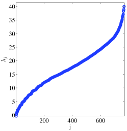
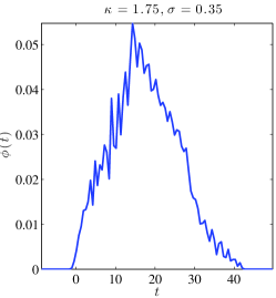
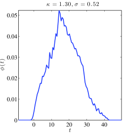
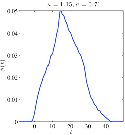
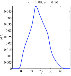
Fig. 1: The eigenvalues, as well as various regularized DOS $\phi_{\sigma}$ obtained by blurring the exact DOS (sum of $\delta$-functions positioned at eigenvalues) of a matrix with Gaussians of the form (5).

We remark that the optimal choice of $\sigma$, and therefore the smoothness of the approximate DOS, is application dependent. On the one hand, $\sigma$ should be chosen to be as large as possible so that the regularized DOS $\phi_{\sigma}$ is easy to approximate numerically. On the other hand, increasing $\sigma$ could cause an undesirable loss of detail and yield an erroneous result. It is up to the user to select a value of $\sigma$ that balances accuracy and efficiency: $\sigma$ should be chosen to be small enough to reach the target accuracy, but not too small which would require a large number of MATVECs to approximate the DOS.

We should also note that  (8) is not the only way to regularize the DOS. Another choice is the Lorentzian function defined as

$$\frac{\eta}{(t-\lambda)^{2}+\eta^{2}}=-\mathrm{Im}\left(\frac{1}{t-\lambda+i\eta}\right),$$ (9)

where $\mathrm{Im}(z)$ denotes the imaginary part of a complex number $z$, and $\eta$ is a small regularization constant that controls the width of the peak centered at $\lambda$. As $\eta$ approaches zero, (9) approaches a Dirac $\delta$-function centered at eigenvalues. This approach is used in Haydock’s method to be discussed in section 3.2.2. We also examine the difference between the regularization procedures in section 4 through numerical experiments.

2.3 Non-negativity condition

Since the DOS can be viewed as a probability distribution function, it satisfies the non-negativity condition in the sense that

$$\langle\phi,g\rangle\geq 0,$$ (10)

for all non-negative function $g(t)\geq 0$ in the Schwartz space. Not all numerical methods described below satisfy the non-negativity condition by construction. We will see in section 4 that the failure of preserving the non-negativity condition can possibly lead to large numerical error.

3 Numerical methods for estimating spectral density

In this section, we review two classes of methods for approximating the DOS of $A$. We begin with the KPM, which can be viewed as a polynomial approximation to the DOS. We show that two other approaches that are derived from different view points are equivalent to KPM. We then describe the second class of methods which are based on the use of the familiar Lanczos partial tridiagonalization procedure [27]. These methods use blurring (or regularization) techniques to construct an approximate DOS from Ritz values. They differ in the type of blurring they utilize. One of them, which we will simply call the Lanczos method uses Gaussian blurring, whereas the other method, which we call the Haydock’s method [20, 3, 31, 5], uses a Lorentzian blurring.

A common characteristic of these methods is that they all use a stochastic sampling and averaging technique to obtain an approximate DOS. The stochastic sampling and averaging technique is based on the following key result [21, 39, 2].

Theorem 1.

Let $A$ be a real symmetric matrix of dimension $n\times n$ with eigen-decomposition $A=\sum_{j=1}^{n}\lambda_{j}u_{j}u_{j}^{T},$ and $u_{i}^{T}u_{j}=\delta_{ij},\quad i,j=1,\cdots,n$. Here $\delta_{ij}$ is the Kronecker $\delta$ symbol. Let $v$ be a vector of dimension $n$, and $v$ can be represented as the linear combination of $\{u_{i}\}_{i=1}^{n}$ as

$$v=\sum_{j=1}^{n}\beta_{j}u_{j}.$$ (11)

If each component of $v$ is obtained independently from a normal distribution with zero mean and unit standard deviation, i.e.

$$\mathbb{E}[v]=0,\quad\mathbb{E}[vv^{T}]=I,$$ (12)

then

$$\mathbb{E}[\beta_{i}\beta_{j}]=\delta_{ij},\quad i,j=1,\cdots,n.$$ (13)

The proof of Theorem 1 is straightforward. The theorem suggest that the trace of a matrix function $f(A)$, which we need to compute in the KPM, for example, can be obtained by simply averaging $v^{T}f(A)v$ for a number of randomly generated vectors $v$ that satisfy the conditions given in (12) because

$$\mathbb{E}[v^{T}f(A)v]=\mathbb{E}[\sum_{j=1}^{n}\beta_{j}^{2}f(\lambda_{j})]=\sum_{j=1}^{n}f(\lambda_{j})=\mbox{Trace}[f(A)].$$ (14)

3.1 The Kernel Polynomial Method

The Kernel Polynomial Method (KPM) was proposed by Silver and Röder [39] and Wang [43] in the mid-1990s to calculate the DOS. See also [40, 41, 11, 33] among others where similar approaches were also used.

3.1.1 Derivation of the origional KPM

The KPM method constructs an approximation to the exact DOS of a matrix $A$ by formally expanding Dirac $\delta$-functions in terms of Chebyshev polynomials $T_{k}(t)=\cos(k\arccos(t))$. For simplicity, we assume that the eigenvalues are in the interval $[-1,1]$. As is the case for all methods which rely on Chebyshev expansions, a change of variables must first be performed to map an interval that contains $[\lambda_{\min},\lambda_{\max}]$ to $[-1,1]$ if this assumption does not hold. Following the Silver-Röder paper [39], we include, for convenience, the inverse of the weight function into the spectral density function,

$$\hat{\phi}(t)=\sqrt{1-t^{2}}\phi(t)=\sqrt{1-t^{2}}\times\frac{1}{n}\sum_{j=1}^{n}\delta(t-\lambda_{j}).$$ (15)

Then we expand the distribution $\hat{\phi}(t)$ as

$$\hat{\phi}(t)=\sum_{k=0}^{\infty}\mu_{k}T_{k}(t).$$ (16)

Eq. (16) should be understood in the sense of distributions, i.e. for any test function $g\in\mathcal{S}$,

$$\int_{-1}^{1}\hat{\phi}(t)g(t)\ dt=\int_{-1}^{1}\sum_{k=0}^{\infty}\mu_{k}T_{k}(t)g(t)\ dt.$$

The same notation applies to the expansion of the DOS using other methods in the following discussion. By means of a formal moment matching procedure, the expansion coefficients $\mu_{k}$ are also defined by

$$\mu_{k} = \frac{2-\delta_{k0}}{\pi}\int_{-1}^{1}\frac{1}{\sqrt{1-t^{2}}}T_{k}(t)\hat{\phi}(t)dt$$ (17)

$$= \frac{2-\delta_{k0}}{\pi}\int_{-1}^{1}\frac{1}{\sqrt{1-t^{2}}}T_{k}(t)\sqrt{1-t^{2}}\phi(t)dt$$

$$= \frac{2-\delta_{k0}}{n\pi}\sum_{j=1}^{n}T_{k}(\lambda_{j}).$$

Here $\delta_{ij}$ is the Kronecker $\delta$ symbol so that $2-\delta_{k0}$ is equal to 1 when $k=0$ and to 2 otherwise.

Thus, apart from the scaling factor $(2-\delta_{k0})/(n\pi)$, $\mu_{k}$ is the trace of $T_{k}(A)$. It follows from Theorem 1 that

$$\zeta_{k}=\frac{1}{n_{\mathrm{vec}}}\sum_{l=1}^{n_{\mathrm{vec}}}\left(v^{(l)}_{0}\right)^{T}T_{k}(A)v^{(l)}_{0}$$ (18)

is a good estimation of the trace of $T_{k}(A)$, for a set of randomly generated vectors $v^{(1)}_{0}$, $v^{(2)}_{0}$, …, $v^{(n_{\mathrm{vec}})}_{0}$ that satisfy the conditions given by  (12). Here the subscript 0 is added to indicate that the vectors have not been multiplied by the matrix $A$. Then $\mu_{k}$ can be estimated by

$$\mu_{k}\approx\frac{2-\delta_{k0}}{n\pi}\zeta_{k},$$ (19)

Now we consider the computation of each term $\left(v^{(l)}_{0}\right)^{T}T_{k}(A)v^{(l)}_{0}$. For simplicity we drop the superscript $l$ and denote by $v_{0}\equiv v^{(l)}_{0}$. The 3-term recurrence of the Chebyshev polynomial is exploited to compute $T_{k}(A)v_{0}$:

$$T_{k+1}(A)v_{0}=2AT_{k}(A)v_{0}-T_{k-1}(A)v_{0}.$$

So if we let $v_{k}\equiv T_{k}(A)v_{0}$, we have

$$v_{k+1}=2Av_{k}-v_{k-1}.$$ (20)

Once the scalars $\{\mu_{k}\}$ are determined, we would in theory get the expansion for $\phi(t)=\frac{1}{\sqrt{1-t^{2}}}\hat{\phi}(t)$. In practice, $\mu_{k}$ decays to $0$ as $k\to\infty$, and the approximate density of states will be limited to Chebyshev polynomials of degree $M$. So $\phi$ is approximated by:

$$\widetilde{\phi}_{M}(t)=\frac{1}{\sqrt{1-t^{2}}}\sum_{k=0}^{M}\mu_{k}T_{k}(t).$$ (21)

For a general matrix $A$ whose eigenvalues are not necessarily in the interval $[-1,1]$, a linear transformation is first applied to $A$ to bring its eigenvalues to the desired interval. Specifically, we will apply the method to the matrix

$$B=\frac{A-cI}{d},$$

where

$$c=\frac{\lambda_{lb}+\lambda_{ub}}{2}\ ,\quad d=\frac{\lambda_{ub}-\lambda_{lb}}{2},$$ (22)

and $\lambda_{lb}$, $\lambda_{ub}$ are lower and upper bounds of the smallest and largest eigenvalues $\lambda_{\min}$ and $\lambda_{\max}$ of $A$ respectively.

It is important to ensure that the eigenvalues of $B$ are within the interval $[-1,1]$. Otherwise the magnitude of the Chebyshev polynomial, hence the product of $T_{k}(B)$ and $v_{0}$ computed through a three-term recurrence, will grow exponentially with $k$.

There are a number of ways [9, 47, 30] to obtain good lower and upper bounds $\lambda_{lb}$ and $\lambda_{ub}$ of the spectrum of $A$. For example, we can set $\lambda_{ub}$ to $\theta_{k}+\|(A-\theta_{k}I)u_{k})\|$, and $\lambda_{lb}$ to $\theta_{1}-\|(A-\theta_{1}I)u_{1})\|$, where $\theta_{1}$ (resp. $\theta_{k}$) is the algebraically smallest (resp. largest) Ritz value obtained from an $k$-step Lanczos iteration and $u_{1}$ (resp. $u_{k}$) is the associated normalized Ritz vector. Note that these residual norms are inexpensive to compute since $\|(A-\theta_{j}I)u_{j}\|$ can be easily expressed from the bottom entry of $z_{j}$, the unit norm eigenvector of the $k\times k$ tridiagonal matrix obtained from the Lanczos process. For details, see Parlett [34, sec. 13.2]. We should point out that $\lambda_{lb}$ and $\lambda_{ub}$ do not have to be very accurate approximations to $\lambda_{\min}$ and $\lambda_{\max}$ respectively. It is demonstrated in [30] that tight bounds can be obtained from a 20-step Lanczos iteration for matrices of dimension larger than 100,000.

Input: Real symmetric matrix $A$ with eigenvalues between $[-1,1]$. A set of points $\{t_{i}\}$ at which DOS is to be evaluated, the degree $M$ of the expansion polynomial. Output: Approximate DOS $\{\widetilde{\phi}_{M}(t_{i})\}$. 1:  Set $\zeta_{k}=0$ for $k=0,\cdots,M$; 2:  for $l=1:n_{\mathrm{vec}}$ do 3:     Select a new random vector $v_{0}^{(l)}$; 4:     for $k=0:M$ do 5:        Compute $\zeta_{k}\leftarrow\zeta_{k}+\left(v_{0}^{(l)}\right)^{T}v_{k}^{(l)}$; 6:        Compute $v_{k+1}^{(l)}$ via the three-term recurrence $v_{k+1}^{(l)}=2Av_{k}^{(l)}-v_{k-1}^{(l)}$  (for $k=0$, $v_{1}^{(l)}=Av_{0}^{(l)}$); 7:     end for 8:  end for 9:  Set $\zeta_{k}\leftarrow\zeta_{k}/n_{\mathrm{vec}},\mu_{k}\leftarrow\frac{2-\delta_{k0}}{n\pi}\zeta_{k}$ for $k=0,1,...,M$; 10:  Evaluate $\{\widetilde{\phi}_{M}(t_{i})\}$ using $\{\mu_{k}\}$ and Eq. (21);

Algorithm 1 The Kernel Polynomial Method.

Because KPM can be viewed as a way to approximate a series of $\delta$-functions which are highly discontinuous, Gibbs oscillation [24] can be observed near the peaks of the spectral density. Fig. 2 shows an approximation to $\delta(t)$ by a Chebyshev polynomial expansion of the form  21 with $M=40$. It can been that the approximation oscillates around 0 away from $t=0$. As a result, it does not preserve the nonnegativity of $\delta(t)$. The Gibbs oscillation can be reduced by a technique called the Jackson damping, which modifies the coefficient of Chebyshev expansion. The details of Jackson damping is given in Appendix A, and Fig. 2 shows that the Jackson damping indeed reduces the amount of Gibbs oscillation significantly. However, Jackson damping tends to oversmooth the approximate DOS and create an approximation to $\delta(t)$ that has a wider spread. We will discuss this again with numerical results in section 4.

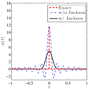
Fig. 2: Chebyshev expansion with and without the Jackson damping for Dirac $\delta$-function $\delta(t)$. The Chebyshev polynomial degree is set to $40$.

We should also point out that it is possible to replace Chebyshev polynomials in KPM by other orthogonal polynomials such as the Legendre polynomials. We will call the variant that uses Legendre polynomials to expand the spectral density by KPML.

We also note that the cost for constructing KPM can be reduced by techniques presented in the Appendix A. Because KPM provides a finite polynomial expansion, the approximate DOS $\widetilde{\phi}$ can be evaluated at any arbitrary point $t$ once the $\mu_{k}^{\prime}s$ have been determined.

3.1.2 The spectroscopic view of KPM

In his 1956 book titled “Applied Analysis” [28], Lanczos described a method for computing spectra of real symmetric matrices, which he termed “spectroscopic”. This approach, which also relies heavily on Chebyshev polynomials, is rather unusual in that it assimilates the spectrum of a matrix to a collection of frequencies and the goal is to detect these frequencies by Fourier analysis. Because it is not competitive with modern methods for computing eigenvalues, this technique has lost its appeal. However, we will show below that the spectroscopic approach is well suited for computing approximate spectral densities, and it is closely connected to the KPM.

Let us assume that the eigenvalues of the matrix $A$ are in [-1,1]. The spectroscopy approach takes samples of a function of the form

$$f(t)=\sum_{j=1}^{n}\beta_{j}^{2}\cos(\theta_{j}t),$$ (23)

where $\theta_{j}$’s are related to eigenvalues of $A$ according to $\theta_{j}=\cos\lambda_{j}$, at $t=0,1,2,...,M$. Then one can take the Fourier transform of $f(t)$ to reveal the spectral density of $A$. If a sufficient number of samples are taken, then the Fourier transform of the sampled function should have peaks near $\cos\lambda_{j}$, $j=1,2,...,n$, and an approximate spectral density can be obtained.

Because $\lambda_{j}$’s are not known, (23) cannot be evaluated directly. However, $M+1$ uniform samples of $f(t)$, i.e. $f(0)$, $f(1)$, …, $f(M)$ can be obtained from the average of

$$v_{0}^{T}v_{0},\>v_{0}^{T}T_{1}(A)v_{0},\>...,\>v_{0}^{T}T_{M}(A)v_{0},$$ (24)

where $T_{k}(t)$ is the same $k$th degree Chebyshev polynomial of the first kind we used in the previous section, and $v_{0}$ is a random starting vector.

Taking a discrete cosine transform of (24) yields

$$F(p)={1\over 2}\left(f(0)+(-1)^{p}f(M)\right)+\sum_{k=1}^{M-1}f(k)\cos\frac{kp\pi}{M},\quad p=0,\cdots,M.$$ (25)

Note that, as is customary, the end values are halved to account for the discontinuity of the data at the interval boundaries. An approximation to the spectral density $\phi(t)$ can be obtained from $F(p)$, $p=0,1,...,M$ through an interpolation procedure.

We now show that the spectroscopic approach is closely connected to KPM. This connection can be seen by noticing that, the coefficient $\zeta_{k}$ in Eq. (18) essentially gives an estimate of the following transform of the spectral density $\phi(t)$

$$f(s)=\int\cos(s\arccos t)\phi(t)dt,$$ (26)

evaluated at an integer $k$.

Since $t\in[-1,1]$, we can rewrite  (26) as the continuous cosine transform of a related function by introducing an auxiliary variable $\xi=\arccos t$, and define

$$\psi(\xi)=\phi(\cos\xi)\sin\xi.$$

It is then easy to verify that  (26) can be written as

$$f(s)=\int_{0}^{\infty}\cos(s\xi)\psi(\xi)\ d\xi.$$

Thus $f(s)$ can indeed by obtained by performing a cosine transform of $\psi(\xi)$.

If $f(s)$ is given, we can obtain $\psi(\xi)$ via the inverse cosine transform

$$\psi(\xi)=\frac{2}{\pi}\int_{0}^{\infty}\cos(s\xi)f(s)\ ds.$$ (27)

Substituting $\xi=\arccos t$ back into (27) yields

$$\phi(t)=\frac{2}{\pi\sqrt{1-t^{2}}}\int_{0}^{\infty}\cos(s\arccos t)f(s)\ ds.$$ (28)

However, since we can only compute $f(s)$ for $s=k,k\in\mathbb{N}$ through estimating the trace of $T_{k}(A)$ by a stochastic averaging technique discussed in section 3.1.1, the integration in (28) can only be performed numerically using, for example, a composite trapezoidal rule:

$$\phi(t)\approx\frac{2}{n\pi\sqrt{1-t^{2}}}\left[\frac{1}{2}f(0)+\sum_{k=1}f(k)T_{k}(t)+\frac{1}{2}f(M)T_{M}(t)\right]$$ (29)

Comparing Eq. (29) with Eq. (16), we find that  (29) is exactly the KPM expansion, except that the coefficient for $T_{M}(t)$ is multiplied by a factor $\frac{1}{2}$. Therefore the spectroscopic method and KPM are essentially equivalent.

3.1.3 The Delta-Gauss-Legendre expansion approach

In some sense, the spectroscopy method discussed in the previous section samples the “reciprocal” space of the spectrum by computing $v_{0}^{T}T_{j}(A)v_{0}$, where $T_{j}(t)$ is the $j$th degree Chebyshev polynomial of the first kind, for a number of different randomly generated vectors $v_{0}$ and $j=0,1,...,M$. It uses the discrete cosine transform to reveal the spectral density. In this section, we examine another way to sample or to probe the spectrum of $A$ at an arbitrary point $t_{i}\in[-1,1]$ directly by computing $\{v_{0}^{T}p_{M_{i}}(A)v_{0}\}$, where $p_{M_{i}}(t)$ is an $M_{i}$th degree polynomial of the form

$$p_{M_{i}}(t)\equiv\sum_{k_{i}=0}^{M_{i}}\mu_{k_{i}}(t_{i})T_{k_{i}}(t).$$ (30)

The expansion coefficient $\mu_{k_{i}}(t_{i})$ in the above expression is chosen, for each $t_{i}$, to be

$$\mu_{k_{i}}(t_{i})=\frac{2-\delta_{k0}}{\pi}\int_{-1}^{1}\frac{1}{\sqrt{1-t^{2}}}T_{k_{i}}(t)\delta(t-t_{i})dt=\frac{2-\delta_{k0}}{\pi}\frac{T_{k_{i}}(t_{i})}{\sqrt{1-t_{i}^{2}}}.$$ (31)

The polynomial $p_{M_{i}}(t)$ defined in (30) can be viewed as a polynomial approximation to the $\delta$-function $\delta(t-t_{i})$, which can be regarded as a spectral probe placed at $t_{i}$.

The reason why $v_{0}^{T}p_{M_{i}}(A)v_{0}$ can be regarded as a sample of the spectral density at $t_{i}$ can be explained as follows. The presence of an eigenvalue at $t_{i}$ can be detected by integrating $\delta(t-t_{i})$ over the entire spectrum of $A$ with respect to a spectral point measure defined at eigenvalues only. The integral returns $+\infty$ if $t_{i}$ is an eigenvalue of $A$ and 0 otherwise. However, in practice, this integration cannot be performed without knowing the eigenvalues of $A$ in advance.

A practical probing scheme can be devised by replacing $\delta(t-t_{i})$ with a polynomial approximation such as the one given in (30), and performing integration, which amounts to evaluating the trace of $p_{M_{i}}(A)$. This trace evaluation can be done by using the same stochastic approach we introduced earlier for the KPM. We call this technique the Delta-Chebyshev method.

If $v_{0}$ is some random vector normalized to have $\|v_{0}\|=1$, whose expansion in the eigenbasis $\{u_{j}\}$ is given by

$$v_{0}=\sum_{j=1}^{n}\beta_{j}u_{j},$$ (32)

then $v_{M_{i}}\equiv p_{M_{i}}(A)v_{0}$ will have the expansion

$$v_{M_{i}}=\sum_{j=1}^{n}\beta_{j}p_{M_{i}}(\lambda_{j})u_{j}.$$ (33)

Taking the inner product between $v_{0}$ and $v_{M_{i}}$ yields

$$(v_{M_{i}})^{T}v_{0}=\sum_{j=1}^{n}\beta_{j}^{2}p_{M_{i}}(\lambda_{j}).$$ (34)

Since $\sum_{j=1}^{n}\beta_{j}^{2}=1$, (34) can be viewed as an integral of $p_{M_{i}}(t)$ associated with a point measure $\{\beta_{j}^{2}\}$ defined at eigenvalues of the matrix $A$. In the case when $\beta_{j}^{2}=1/n$ for all $j$, we can then simply rewrite the integral as $\mbox{Trace}[p_{M_{i}}(A)]/n$. As we have already shown in previous sections, such a trace can be approximated by choosing multiple random vectors $v_{0}$ that satisfy the conditions (12) and averaging $v_{0}^{T}p_{M_{i}}(A)v_{0}$ for all these vectors. The averaged value yields $\widetilde{\phi}(t_{i})$, which is the approximation to the spectral density $\phi(t)$ at an arbitrary sample point $t_{i}$.

As we already indicated in section 2, because $\delta(t-t_{i})$ is not a proper function, constructing a good polynomial approximation directly may be difficult. A more plausible approach is to “regularize” $\delta(t-t_{i})$ first by replacing it with a smooth function that has a peak at $t=t_{i}$, and constructing a polynomial approximation to this smooth function.

We choose the regularized $\delta$-function to be the Gaussian $g_{\sigma}(t-t_{i})$, where $g_{\sigma}$ is defined in (5), and the standard deviation $\sigma$ controls the smoothness or the amount of regularization of the function.

It is possible to expand $g_{\sigma}(t-t_{i})$ in terms of Chebyshev polynomials. However, we found that it is easier to derive an expansion in terms of Legendre polynomials. It can been shown (see Appendix A) that

$$g_{\sigma}(t-t_{i})=\frac{1}{(2\pi\sigma^{2})^{1/2}}\sum_{k=0}^{\infty}\left(k+\frac{1}{2}\right)\gamma_{k}(t_{i})L_{k}(t)\,$$ (35)

where $L_{k}(t)$ is the Legendre polynomial of degree $k$, and the expansion coefficient $\gamma_{k}(t_{i})$ is defined by

$$\gamma_{k}(t_{i})=\ \int_{-1}^{1}L_{k}(s)e^{-{1\over 2}((s-t_{i})/\sigma)^{2}}ds.$$ (36)

It can be also shown (see Appendix A) that $\gamma_{k}(t_{i})$ can be determined by a recursive procedure that does not require explicitly to compute the integral in (36).

If we take an approximation to $g_{\sigma}(t-t_{i})$ to be the first $M_{i}+1$ terms in the expansion (35), i.e.,

$$\tilde{\phi}_{M_{i}}(t)=\frac{1}{(2\pi\sigma^{2})^{1/2}}\sum_{k=0}^{M_{i}}\left(k+\frac{1}{2}\right)\gamma_{k}(t_{i})L_{k}(t),$$ (37)

then a practical scheme for sampling the spectral density of $A$ can be devised by computing $v_{0}^{T}h_{M_{i}}(A)v_{0}$ for randomly generated and normalized $v_{0}$’s and averaging these quantities. Because this scheme is based on regularizing the $\delta$ function with a Gaussian and expanding the Gaussian in Legendre polynomials, we call this scheme a Delta-Gauss-Legendre (DGL) method and summarize this scheme in Algorithm 2.

Input: Real symmetric matrix $A$ with eigenvalues between $[-1,1]$. A set of points $\{t_{i}\}$ at which the DOS is to be evaluated, and $M_{\max}$ is the maximum degree employed for all the points. Output: Approximate DOS $\{\widetilde{\phi}_{M}(t_{i})\}$. 1:  for each $t_{i}$ do 2:     Compute and store the expansion coefficients $\{\gamma_{k}(t_{i})\}_{k=0}^{M_{i}}$ using Eq. (36); 3:  end for 4:  Set $\zeta_{k}=0$ for $k=0,\cdots,M_{\max}$; 5:  for $l=1:n_{\mathrm{vec}}$ do 6:     Select a new random vector $v_{0}^{(l)}$; 7:     for $k=0:M_{\max}$ do 8:        Compute $\zeta_{k}\leftarrow\zeta_{k}+\left(v_{0}^{(l)}\right)^{T}v_{k}^{(l)}$; 9:        Compute $v_{k+1}^{(l)}$ via the three-term recurrence $v_{k+1}^{(l)}=\frac{2k+1}{k+1}Av_{k}^{(l)}-\frac{k}{k+1}v_{k-1}^{(l)}$  (for $k=0$, $v_{1}^{(l)}=Av_{0}^{(l)}$); 10:     end for 11:  end for 12:  Set $\zeta_{k}\leftarrow\zeta_{k}/n_{\mathrm{vec}}$ for all $k=0,1,...,M_{\max}$; 113:  Evaluate $\widetilde{\phi}_{M_{i}}(t_{i})$ using Eq. (37) with $\{\zeta_{k}\}$ and the stored $\{\gamma_{k}(t_{i})\}$;

Algorithm 2 Multi-point Delta-Gauss-Legendre expansion.

Note that both the Delta-Chebyshev and the DGL methods compute $v_{0}^{T}p_{M_{i}}v_{0}$ at sampled point $t_{i}$ within the spectrum of $A$. This would have been an unacceptably expensive procedure if it were not for the fact that the same vector sequence $\{T_{k}(A)v_{0}\}$ and $\{L_{k}(A)v_{0}\}$ for $k=0,1,...$, can be used for all points $t_{i}$ at the same time. They only need to be generated once.

Although the Delta-Chebyshev method and KPM are derived from somewhat different principles, there is a close connection between the two, which may not be entirely obvious. The key to recognizing this connection is to notice that the average value of $v_{0}^{T}p_{M_{i}}(A)v_{0}$ can be viewed as an approximation to $\mbox{Trace}(p_{M_{i}}(A))$, which can be written as

$$\mbox{Trace}(p_{M_{i}}(A)) = \frac{1}{n}\sum_{k_{i}=0}^{M_{i}}\mu_{k_{i}}(t_{i})\sum_{j=1}^{n}T_{k_{i}}(\lambda_{j})$$ (38)

$$= \frac{1}{n}\sum_{k_{i}=0}^{M_{i}}\frac{2-\delta_{k_{i},0}}{\pi}\frac{T_{k_{i}}(t_{i})}{\sqrt{1-t_{i}^{2}}}\mbox{Trace}(T_{k_{i}}(A))$$

$$= \sum_{k_{i}=0}^{M_{i}}\left[\frac{2-\delta_{k_{i},0}}{n\pi}\mbox{Trace}(T_{k_{i}}(A))\right]\frac{T_{k_{i}}(t_{i})}{\sqrt{1-t_{i}^{2}}}.$$

Note that the coefficients within the square bracket in (38) are exactly the same coefficients as in KPM, which appear in the expansion (16) of the function $\hat{\phi}(t)=\sqrt{1-t^{2}}\phi(t)$. Therefore, when $M_{i}=M$ for all $i$, the Delta-Chebyshev expansion method is identical to the KPM. Hence, the cost of this approach is the same as that of KPM if polynomials of the same degree and the same number of sampling vectors are used at each $t_{i}$.

When $M_{i}$ is allowed to vary with respect to $i$, there is a slight advantage of using the Delta-Chebyshev method in terms of flexibility. We can use polynomials of different degrees in different parts of the spectrum to obtain a more accurate approximation. Note that in this situation, if $M_{\max}$ is the maximum degree employed for all the points, the number of MATVECs employed remains the same and equal to $M_{\max}$, since we will need to compute for each random vector $v_{0}$, the vectors $T_{k}(A)v_{0}$ for $k=0,\cdots,M_{\max}$ as these are needed by the points requiring the highest degree. However, some of the other calculations (inner products) required to obtain the spectral density can be avoided, though in most cases applying $T_{k}(A)$ to $v_{0}$ dominate the computational cost in the DOS calculation. The computational cost of DGL is similar to that of the Delta-Chebyshev method. Similarly, one can also show that DGL is closely related to KPML, i.e., it is expansion of a regularized spectral density in terms of Legendre polynomials. However, we will omit the alternative derivation here.

The close connection between the Delta-Chebyshev method and KPM also suggests that Gibbs oscillation can be observed in the approximate DOS produced by Delta-Chebyshev and DGL, especially when $\sigma$ is small. There is no guarantee that the non-negativity of $\phi(t)$ can be preserved by DGL.

3.2 The Lanczos Algorithm

Because finding a highly accurate DOS essentially amounts to computing all eigenvalues of $A$, any method that can provide approximations to the spectrum of $A$ can be used to construct an approximate DOS as well. Since the Lanczos algorithm yields good approximation to extreme eigenvalues, it is a good candidate for computing localized spectral densities at least at both ends of the spectrum. In this section, we show that it is also possible to combine the Lanczos algorithm with multiple randomly generated starting vectors to construct a good approximation to the complete DOS.

It should be noted that the spectral density $\phi$ as a probability distribution is non-negative, i.e. $\langle\phi,g\rangle\geq 0$ if $g\geq 0$ everywhere. This is an important property, but the KPM and its variants as introduced in previous sections do not preserve the non-negativity of the spectral density. In contrast, the methods introduced in this section, including the Lanczos method and the Haydock method do preserve the non-negativity by construction. This will become a clear advantage for certain spectral densities as will be illustrated in section 4 through numerical experiments.

3.2.1 Constructing spectral density approximating from Ritz values and Gaussian blurring

For a given starting vector $v_{0}$, an $M$-step Lanczos procedure for a real symmetric matrix $A$ can be succinctly described by

$$AV_{M}=V_{M}T_{M}+f_{M}e_{M}^{T},\ \ V_{M}^{T}V_{M}=I,\ \ V_{M}^{T}f_{M}=0.$$ (39)

Here $T_{M}$ is an $M\times M$ tridiagonal matrix, $V_{M}$ is an $n\times M$ matrix, and $I_{M}$ is an $M\times M$ identity matrix. It is well known that [18] the $k$-th column of $V_{M}$ can be expressed as

$$V_{M}e_{k}=p_{k-1}(A)v_{0},\quad k=1,\cdots,M.$$

where $\{p_{k}(t)\}$, $k=0,1,2,..,M-1$ is a set of polynomials orthogonal with respect to the weighted spectral distribution $\phi_{v_{0}}(t)$ that takes the form

$$\phi_{v_{0}}(t)=\sum_{j=1}^{n}\beta_{j}^{2}\delta(t-\lambda_{j}),$$ (40)

where $\beta_{j}$’s are the expansion coefficients obtained from expanding $v_{0}$ in the eigenvector basis of $A$ as in Eq. (32).

It is also well known that these orthogonal polynomials can be generated by a three-term recurrence whose coefficients are defined by the matrix elements of $T_{M}$ [15]. If $(\theta_{k},y_{k})$, $k=0,1,2,\ldots,M$ are eigenpairs of the tridiagonal matrix $T_{M}$, and $\tau_{k}$ is the first entry of $y_{k}$, then the following distribution function defined by

$$\sum_{k=0}^{M}\tau_{k}^{2}\delta(t-\theta_{k}),$$ (41)

serves as an approximation to the weighted spectral density function $\phi_{v_{0}}(t)$, in the sense that

$$\sum_{j=1}^{n}\beta_{j}^{2}p_{q}(\lambda_{j})=\sum_{k=0}^{M}\tau_{k}^{2}p_{q}(\theta_{k}),$$ (42)

for all polynomials of degree $0\leq q\leq 2M+1$. The moment matching property described by (42) is well known [17], and is related to the Gaussian quadrature rules [16, 19, 18].

Since in most cases, we are interested in the standard spectral density defined by (1), we would like to choose a starting vector $v_{0}$ such that $\beta_{j}^{2}$ is uniform. However, this is generally not possible without knowing the eigenvectors $\{u_{j}\}$ of $A$ in advance. To address this issue, we resort to the same stochastic approach we used in previous sections.

We repeat the Lanczos process with multiple randomly generated starting vectors $v^{(l)}_{0}$, $l=1,2,\ldots,n_{\mathrm{vec}}$, that satisfy the conditions given by (12). It follows from (14) that

$$\frac{1}{n_{\mathrm{vec}}n}\sum_{l=1}^{n_{\mathrm{vec}}}\left(v^{(l)}_{0}\right)^{T}\delta(tI-A)v^{(l)}_{0}=\frac{1}{n}\sum_{j=1}^{n}\left(\frac{1}{n_{\mathrm{vec}}}\sum_{l=1}^{n_{\mathrm{vec}}}\left(\beta_{j}^{(l)}\right)^{2}\right)\delta(t-\lambda_{j})$$ (43)

is a good approximation to the standard spectral density $\phi(t)$ in Eq. (1). Since each distribution (41) generated by the Lanczos procedure is a good approximation to (40), the average of (41) over $l$, i.e.,

$$\widetilde{\phi}(t)=\frac{1}{n_{\mathrm{vec}}}\sum_{l=1}^{n_{\mathrm{vec}}}\left(\frac{1}{n}\sum_{k=0}^{M}\left(\tau_{k}^{(l)}\right)^{2}\delta(t-\theta_{k}^{(l)})\right)$$ (44)

should yield a good approximation to the standard spectral density (1).

Since (44) has far fewer peaks than $\phi(t)$, when $M$ is small, a direct comparison of (44) with $\phi(t)$ is not very meaningful. However, when $\phi(t)$ is regularized by replacing $\delta(t-\lambda_{i})$ with $g_{\sigma}(t-\lambda_{i})$, we can replace $\delta(t-\theta_{k}^{(l)})$ in (44) with a Gaussian centered at the $\theta_{k}^{(l)}$ to yield a regularized DOS approximation, i.e., we define the approximate DOS as

$$\widetilde{\phi}_{\sigma}(t)=\frac{1}{n_{\mathrm{vec}}}\sum_{l=1}^{n_{\mathrm{vec}}}\left(\frac{1}{n}\sum_{k=0}^{M}\left(\tau_{k}^{(l)}\right)^{2}g_{\sigma}(t-\theta_{k}^{(l)})\right).$$ (45)

This regularization is well justified because in the limit of $M=n$, all Ritz values are the eigenvalues, and $\widetilde{\phi}_{\sigma}(t)$ is exactly the same as the regularized DOS $\phi_{\sigma}(t)$ for the same $\sigma$. We will refer to the method that constructs the DOS approximation from Ritz values obtained from an $M$-step Lanczos iteration as the Lanczos method in the following discussion.

Because $g_{\sigma}(t)\geq 0$, the approximate DOS produced by the Lanczos method is nonnegative. This is a desirable property not shared by KPM, the DGL or the spectroscopic method.

An alternative way to refine the Lanczos based DOS approximation from a $M$-step Lanczos run is to first construct an approximate cumulative spectral density or cumulative density of states (CDOS), which is a monotonically increasing function and then take the derivative of the CDOS through a finite difference procedure or other means. This technique is discussed in Appendix C.

3.2.2 Haydock’s method

As we indicated earlier, the use of Gaussians is not the only way to regularize the spectral density. Another possibility is to replace $\delta(t-\lambda_{i})$ in (2) with a Lorentzian of the form (9) and centered at $\lambda_{i}$. The regularized DOS can be written as

$$\phi_{\eta}(t)=\frac{1}{n\pi}\sum_{j=1}^{n}\frac{\eta}{(t-\lambda_{j})^{2}+\eta^{2}}.$$

Consequently, an alternative approximation to the spectral density can be obtained by simply replacing $\delta(t-\theta_{k}^{(k)})$ in (44) with a Lorentzian centered at $\theta_{k}^{(k)}$, i.e.,

$$\widetilde{\phi}_{\eta}(t)=\frac{1}{n_{\mathrm{vec}}}\sum_{l=1}^{n_{\mathrm{vec}}}\left[\frac{1}{n}\sum_{k=0}^{M}\left(\tau_{k}^{(l)}\right)^{2}\frac{\eta}{(t-\theta_{k}^{(l)})^{2}+\eta^{2}}\right],$$

where $\theta_{k}^{(l)}$ and $\tau_{k}^{(l)}$ are the same Ritz values and weighting factors that appear in (45) and $\eta$ is an appropriately chosen constant that corresponds to the resolution of the spectral density to be approximate. This approximation was first suggested by Haydock, Heine and Kelly [20]. We will refer to this approach as Haydock’s method.

Haydock’s original method does not require computing Ritz values even though computing the eigenvalues of a small tridiagonal matrix is by no means costly nowadays. The method makes use of the fact that

$$\phi_{\eta}(t)=-\frac{1}{n\pi}\mathrm{Im}~{}\sum_{j=1}^{n}\frac{1}{t-\lambda_{j}+i\eta}=\frac{1}{n\pi}\mathrm{Im}~{}\mbox{Trace}\left[(tI-A+i\eta I)^{-1}\right].$$

Hence, once again, the task of approximating $\phi_{\eta}(t)$ reduces to that of approximating the trace of $(tI-A+i\eta I)^{-1}$, which can be obtained by

$$\frac{1}{n_{\mathrm{vec}}}\sum_{l=1}^{n_{\mathrm{vec}}}\left(v_{0}^{(l)}\right)^{T}(tI-A+i\eta I)^{-1}v_{0}^{(l)},$$ (46)

for ${n_{\mathrm{vec}}}$ randomly generated vectors $v_{0}^{(l)}$ that satisfy the conditions (12).

Note that a direct calculation of (46) requires solving linear systems of the form $[A-(t+i\eta)I]z=v_{0}$ repeatedly for any point $t$ at which the spectral density is to be evaluated. This approach can be prohibitively expensive. Haydock’s approach approximates $v_{0}^{T}(tI-A+i\eta I)^{-1}v_{0}$ for multiple $t$’s at the cost of performing a single Lanczos factorization and some additional calculations that are much lower in complexity.

If $v_{0}$ is used as the starting vector of the Lanczos procedure, then it follows from the shift-invariant property of the Lanczos algorithm that

$$[A-(t+i\eta)I]V_{M}=V_{M}[T_{M}-(t+i\eta)I]+fe_{M+1}^{T},$$ (47)

where $V_{M}$ and $T_{M}$ are the same orthonormal and tridiagonal matrices respectively that appear in (39). After multiplying  (47) from the left by $[A-(t+i\eta)I]^{-1}$, from the right by $[T_{M}-(t+i\eta)I]^{-1}$ and rearranging terms, we obtain

$$[A-(t+i\eta)I]^{-1}V_{M}=V_{M}[T_{M}-(t+i\eta)I]^{-1}-[A-(t+i\eta)I]^{-1}fe_{M+1}^{T}[T_{M}-(t+i\eta)I]^{-1}.$$

It follows that

$$v_{0}^{T}\left[A-(t+i\eta)I\right])^{-1}v_{0} = e_{1}^{T}V_{M}^{T}[A-(t+i\eta)I]^{-1}V_{M}e_{1}$$

$$= e_{1}^{T}[T_{M}-(t+i\eta)I]^{-1}e_{1}+\xi,$$

where $\xi=-\left(v_{0}^{T}[A-(t+i\eta)I]^{-1}f\right)\left(e_{M+1}^{T}[T_{M}-(t+i\eta)I]^{-1}e_{1}\right)$. If $\xi$ is sufficiently small, computing $v_{0}^{T}(tI-A+i\eta I)^{-1}v_{0}$ reduces to computing the $(1,1)$-th entry of the inverse of $T_{M}-(t+i\eta)I$. It is not difficult to show that this entry is exactly the same as the expression given in (46) up to a constant scaling factor.

Because $T_{M}$ is tridiagonal with $\alpha_{1},\alpha_{2},...,\alpha_{M}$ on the diagonal and $\beta_{2},\beta_{3},...,\beta_{M}$ on the sub-diagonals and super-diagonals, $e_{1}^{T}(zI-T_{M})^{-1}e_{1}$ can be computed in a recursive fashion using a continued fraction formula

$$e_{1}^{T}(zI-T_{M})^{-1}e_{1}=\frac{1}{z-\alpha_{1}+\frac{\beta_{2}^{2}}{z-\alpha_{2}+\cdots}}.$$ (48)

This formula can be verified from the identity

$$\left(z-T_{M}\right)^{-1}_{1,1}\equiv\frac{\det(zI-T_{M})}{\det(z-\hat{T}_{M})}$$

where $\hat{T}_{M}$ is the trailing submatrix starting from the $(2,2)$ entry of $T_{M}$ (48) and tridiagonal structure of both $T_{M}$ and $\hat{T}_{M}$ matrices.

It is also related to the generation of Sturm sequences which is used in bisection methods for computing eigenvalues of tridiagonal matrices [34]. Although this is an elegant way to compute $e_{1}^{T}(T_{M}-zI)^{-1}e_{1}$, its cost is not much lower than that of solving the linear system $(T_{M}-zI)w=e_{1}$ and taking its first entry. For most problems, the cost for this procedure is small compared to that required to perform the Lanczos procedure to obtain $T_{M}$.

We should point out that the non-negativity of $\phi(t)$ is preserved by the Haydock method. However, the Lorentzian function defined by (9) decreases to 0 at a much slower rate compared to a Gaussian as $t$ moves away from $\lambda$. Hence, when a high resolution approximation is needed, we may need to choose a very small $\eta$ in order to produce an accurate approximation.

4 Numerical results

In this section, we compare all methods discussed above for approximating the spectral density of $A$ through numerical examples. For a given test problem, we first define the target resolution of the DOS to be approximated by setting the parameter $\sigma$ in either (4) or (6) or the parameter $\eta$ in (9). We use the metric defined in Eq. (6) to measure the approximation errors associated with KPM and its variants with the exception of DGL. For DGL, Lanczos and Haydock methods, we simply use the error metric (4) with $p=\infty$. Since the spectroscopic method is equivalent to KPM, we do not show any numerical results for the spectroscopic method.

4.1 Modified Laplacian matrix

The first example is a modified 2D Laplacian operator with zero Dirichlet boundary condition defined on the domain $[0,30]\times[0,30]$. The operator is discretized using a five-point finite difference stencil with $\Delta h=1$. The modification involves adding a diagonal matrix, which can be regarded as a discretized potential function. The diagonal matrix is generated by adding two Gaussians, one centered at the point (4,5) of the domain and the other at the point (25,15). The dimension of the matrix is $750$, which is relatively small. We set the parameter $\sigma$ and $\eta$ to $0.35$. For all calculations shown in this section, we use $n_{\mathrm{vec}}=100$ random vectors whenever stochastic averaging is needed. Each calculation is repeated $10$ times. Each plotted value is the mean value of the computed quantities produced from the $10$ runs, with the error bar indicating the standard deviation of the $10$ runs.

In Fig. 3, we compare all methods presented in the previous section. We observe that the Lanczos method seems to outperform all other methods, especially when $M$ is relatively small. The use of Jackson damping in KPM does not appear to improve the accuracy of the approximation. To some extent, this is not surprising because the true DOS has many sharp peaks (see Fig. 4) even after it is regularized. Hence, using Jackson damping, which tends to over-regularize the KPM approximation, may not be able to capture these sharp peaks. The DGL method, the KPM and KPML behave similarly, as is expected.

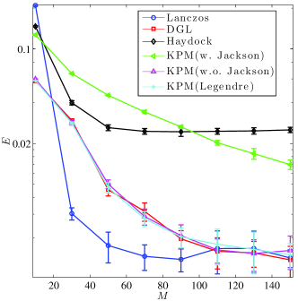
Fig. 3: A comparison of approximation errors of all methods applied to the modified Laplacian matrix for different $M$ values.

In Fig. 4, we compare $\phi_{\sigma}(t)$ and $\widetilde{\phi}(t)$ directly for the Lanczos, Haydock, KPM with and without Jackson damping. To see the accuracy of different methods more clearly, we choose a higher resolution by setting $\sigma$ and $\eta$ to $0.05$. We note that the meaning of $\widetilde{\phi}(t)$ is different for different methods. For Lanczos, $\widetilde{\phi}(t)$ is the approximate DOS obtained using the Gaussian blurring. For Haydock, $\widetilde{\phi}(t)$ is the approximate DOS obtained using the Lorentzian Gaussian blurring. For KPM (with and without Jackson damping), we first evaluate $\widetilde{\phi}(t)$ as in section 3.1, and then plot instead the quantity $\langle\widetilde{\phi}(\cdot),g_{\sigma}(\cdot-t)\rangle$. In this sense, the exact and approximate DOS are regularized on the same footing. The same procedure is adopted for other numerical examples in this section as well.

We use $M=100,n_{\mathrm{vec}}=100$ for all methods. In this case, a visual inspection of the approximate DOS plots in Fig. 4 yields the same conclusion that we reached earlier based on the measured errors shown in Fig. 3. Lanczos appears to be the most accurate among all methods. The DOS curves generated from both the Lanczos and the Haydock methods are above zero. The peaks in the DOS curve produced by the Haydock method are not as sharp as those produced by the Lanczos method. This is because Haydock uses a Lorentzian to regularize the Dirac $\delta$-function, whereas the Lanczos method uses a Gaussian function to blur the Dirac $\delta$-function centered at Ritz values. The KPM method without Jackson damping does not preserve the non-negativity of the approximate DOS, and Gibbs oscillation is clearly observed in Fig. 4 (d). Finally, KPM with Jackson damping preserves the non-negativity of the approximate DOS. However, the use of Jackson damping leads to missing several peaks in the DOS, as is illustrated in Fig. 3. The behavior of DGL and KPML are similar to that of KPM without Jackson damping.

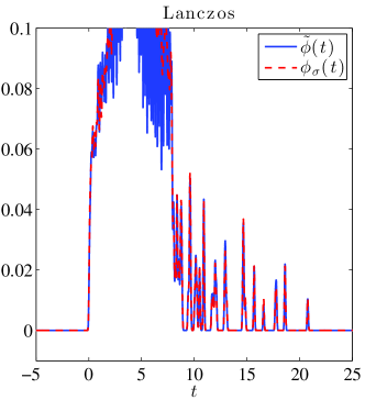
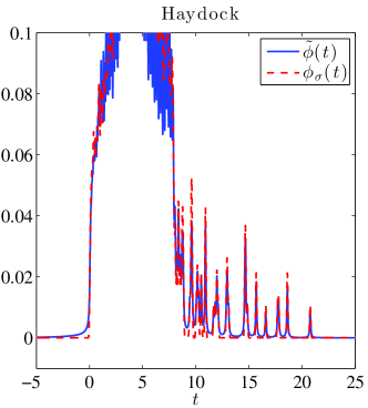
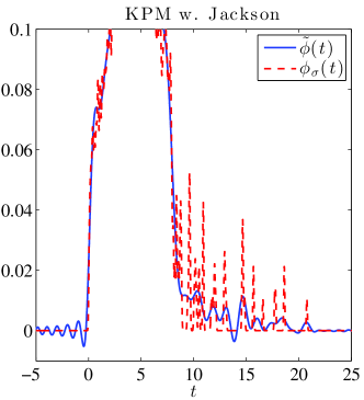
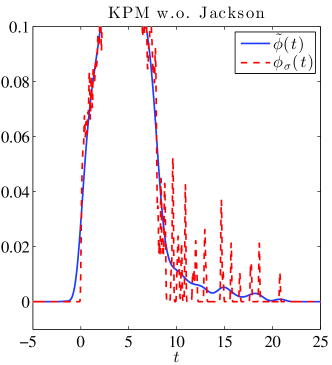
Fig. 4: Comparing the regularized DOS (with $\sigma=0.05$) with the approximate DOS produced by (a) the Lanczos method (b) the Haydock method (c) the KPM with Jackson damping (d) the KPM without Jackson damping for $M=100$.

4.2 Other test matrices

In this section, we compare different DOS approximation methods for two other matrices taken from the Univerisity of Florida Sparse Matrix collection [8]. The pe3k matrix originates from vibrational mode calculation of a polyethylene molecule with 3,000 atoms [46]. The shwater matrix originates from a computational fluid dynamics simulation. The size of the pe3k matrix is 9,000, and the size of shwater matrix is 81,920. These two test matrices have quite different characteristics in their DOS. The spectrum of the pe3k matrix contains a large gap as well as many peaks. The DOS of the shwater matrix is relatively smooth as we will see below.

We set $\sigma$ to $0.3$ in tests presented in this section. We observe that KPM with Jackson damping only becomes accurate when the degree of the expanding polynomials ($M$) is high enough, and the convergence with respect to $M$ is rather slow. The DGL method, KPM without Jackson damping and KPML behave similarly.

For the shwater matrix, which has a relatively smooth spectral density, the Lanczos method is still the most accurate. It only take $M=50$ Lanczos steps to reach $10^{-3}$ accuracy. The KPM (without Jackson damping) and KPML, as well as the DGL method all require $M>110$ terms to reach the same level of accuracy.

Fig. 6 shows that when we set $M=100$, $n_{\mathrm{vec}}=100$, the KPM without Jackson damping yields accurate approximation to the DOS, whereas the Jackson damping introduces slightly larger error near the locations of the peaks and valleys of the DOS curve. This error is due to the use of extra smoothing. The DOS generated by the Haydock method also has larger error near the peaks and valleys of the DOS curves. This is due to the use of Lorentzian regularization.

In Fig. 7, we zoom into the tail of the DOS curves produced by the Lanczos and KPM. It can be seen that Lanczos preserves the non-negativity of the DOS, whereas KPM does not. However, since the DOS is smooth, the Gibbs oscillation is very small, and can only be seen clearly at the tail of the DOS curve.

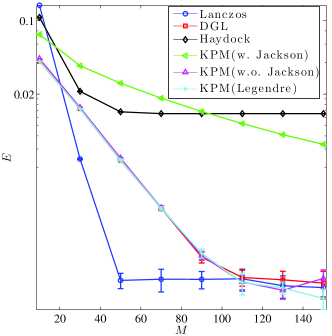
Fig. 5: A comparision of approximation errors of all DOS approximation methods applied to the shwater matrix for different $M$ values. The regularization parameter $\sigma$ is set to 0.3.

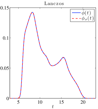
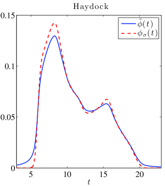
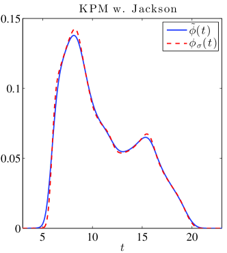
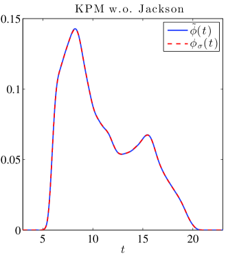
Fig. 6: Comparing the regularized DOS (with $\sigma=0.3$) with the approximate DOS produced by (a) the Lanczos method (b) the Haydock method (c) the KPM with Jackson damping (d) the KPM without Jackson damping for the shwater matrix.

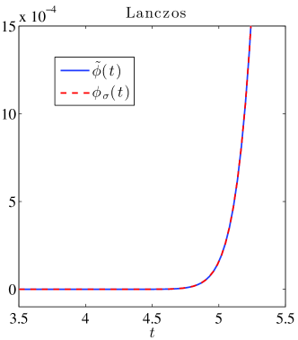
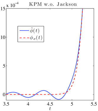
Fig. 7: A comparison of approximation errors of the Lanczos method (a) with that of the KPM without Jackson damping (b) at the higher end of the spectrum of the shwater matrix.

For the pe3k matrix, Fig. 8 shows that the Lanczos method is significantly more accurate than other methods, followed by the Haydock method. This difference in accuracy can be further observed in Fig. 9, which compares the regularized DOS with the approximate DOS for the Lanczos method, the Haydock method, and the KPM with and without Jackson damping. We use $M=100$ and $n_{\mathrm{vec}}=100$. The pe3k matrix has a large gap between the low and high ends of the spectrum. Without the use of Jackson damping, the KPM produces large oscillations over the entire spectrum. We observed similar behavior for DGL and KPML. Adding Jackson damping reduces oscillation in the approximate DOS. However, it leads to an over-regularized DOS approximation and is not accurate.

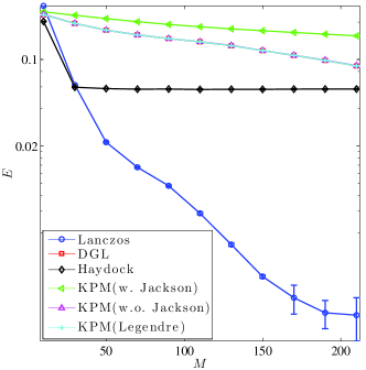
Fig. 8: A comparison of approximation errors of all DOS approximation methods applied to the pe3k matrix for different $M$ values. The regularization parameter $\sigma$ is set to 0.3.

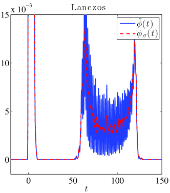
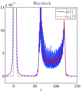
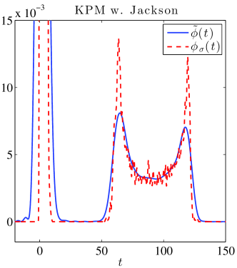
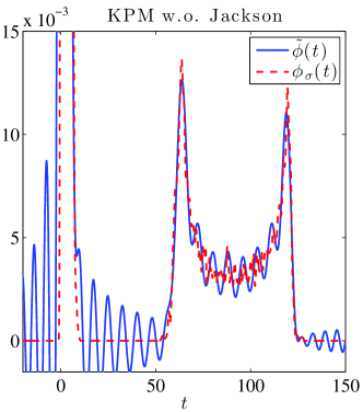
Fig. 9: Comparing the regularized DOS (with $\sigma=0.3$) with the approximate DOS produced by (a) the Lanczos method (b) the Haydock method (c) the KPM with Jackson damping (d) the KPM without Jackson damping for the pe3k matrix.

4.3 Application: Heat capacity calculation

At the end of section 2.1 we discussed that there are different ways for regularizing the DOS depending on the applications. Here we give an example of the calculation of the heat capacity of a molecule. The heat capacity is a thermodynamic property and is defined as [32, 45]

$$C_{v}=\int_{0}^{\infty}k_{B}\frac{(\hbar\omega c/k_{B}T)^{2}e^{-\hbar\omega c/k_{B}T}}{(1-e^{-\hbar\omega c/k_{B}T})^{2}}\phi(\omega)d\omega,$$ (49)

where $k_{B}$ is the Boltzmann constant, $c$ is the speed of light, $\hbar$ is Planck’s constant, $T$ is the temperature and $\omega=\sqrt{\lambda}$ is the vibration frequency.

Here, if we define

$$g(\omega)=k_{B}\frac{(\hbar\omega c/k_{B}T)^{2}e^{-\hbar\omega c/k_{B}T}}{(1-e^{-\hbar\omega c/k_{B}T})^{2}},$$ (50)

and define the DOS $\phi(\omega)$ using the square root of the eigenvalues of the Hessian associated with a molecular potential function with respect to atomic coordinates of the molecule, we have

$$C_{v}=\langle\phi,g\rangle.$$

Therefore the error can be measured directly using Eq. (7).

In the following, we take the Hessian to be the modified Laplacian matrix and the pe3k matrix, and compute the corresponding heat capacity $C_{v}(T)$ for different temperature values $T$. We note that here the computed values of $C_{v}(T)$ do not carry any physical meaning. They merely serve as a proof of principle for assessing the accuracy of the estimated DOS. We compare the KPM and the Lanczos method. All computations are done using $M=40$ MATVECs. Each computed $C_{v}$ is an averaged value over $100$ runs. To facilitate the comparison, we normalize $C_{v}$ so that its maximum value is $1$. The Lanczos method is also fully flexible when the error metric is changed. To this end we regularize the distribution obtained from Ritz values not by Gaussians, but by the function $g$ in this application. In other words, in Eq. (45) we replace $g_{\sigma}$ by the function $g$ in Eq. (50).

Fig. 10 shows that both the KPM and the Lanczos method correctly reproduce the normalized $C_{v}(T)$ for the modified Laplacian matrix. We also plot the error generated in both the KPM and the Lanczos method. We observe that the error associated with the Lanczos method is slightly smaller. This observation agrees with previous results that demonstrate the effectiveness and accuracy of both the KPM and the Lanczos methods for computing a relatively smooth DOS.

Fig. 11 shows that, for the pe3k matrix, the KPM approximation of $C_{v}(T)$ exhibits much larger error than that produced by the Lanczos method. This observation agrees with the results shown in Figure 9, which suggests that the Lanczos method yields a much more accurate DOS estimate, especially when $M$ is relatively small.

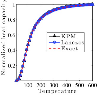
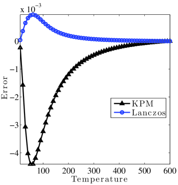
Fig. 10: A comparison of the approximate heat capacity produced by the Lanczos and the KPM with the “exact” heat capacity at different temperatures (left) , and the approximation errors produced by these methods at different temperature values (right) for the modified Laplacian.

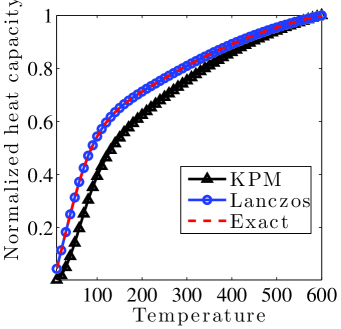
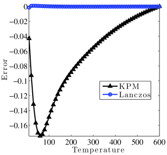
Fig. 11: A comparison of the approximate heat capacity produced by the Lanczos and the KPM with the “exact” heat capacity at different temperatures (left) , and the approximation errors produced by these methods at different temperature values (right) for the pe3k matrix.

5 Conclusion

We surveyed numerical algorithms for estimating the spectral density of a real symmetric matrix $A$ from a numerical linear algebra perspective. The algorithms can be categorized into two classes. The first class contains the KPM method an its variants. The KPM is based on constructing polynomial approximations to Dirac $\delta$-“functions” or regularized $\delta$-“functions”. We showed that the Lanczos spectroscopic method is equivalent to KPM even though it is derived from different view points. The DGL method is slightly different, but can be viewed as a polynomial expansion of a regularized spectral density. It is more flexible because it allows polynomials of different degrees to be used at different spectral locations.

The second class of methods is based on the classical Lanczos procedure for partially tridiagonalizing $A$. Both the Lanczos and the Haydock methods make use of eigenvalues and eigenvectors of the tridiagonal matrix to construct approximations to the DOS. They only differ in the type of regularization they use to interpolate spectral density from Ritz values to other locations in the spectrum. The Lanczos method uses a Gaussian blurring function, whereas the Haydock method uses a Lorentzian. Because a Lorentzian decreases to zero at a much slower rate than a Gaussian away from its peak, it is less effective when a high resolution spectral density is needed.

Regularization through the use of Gaussian blurring of $\delta$-“functions” not only allows us to specify the desired resolution of the approximation, but also allows us to properly define an error metric for measuring the accuracy of the approximation in a rigorous and quantitative manner.

The KPM and its variants require estimating the trace of $A$ or $p(A)$ where $p(t)$ is a polynomial. An important technique for obtaining such an estimate is the stochastic sampling and averaging of the Rayleigh quotient $v_{0}^{T}p(A)v_{0}/v_{0}^{T}v_{0}$. Averaging the tridiagonal matrices produced by the Lanczos procedure started from randomly generated starting vectors ensures that the approximation contains equal contributions from all spectral components of $A$. This is an important requirement of the Lanczos and Haydock algorithms.

Our numerical tests show that the Lanczos method consistently outperforms other methods in term of the accuracy of the approximation, especially when a few MATVECs are used in the computation. Furthermore, both the Lanczos and Haydock algorithms guarantee that the approximate DOS is non-negative. This is a desirable feature of any DOS approximation. Another nice property of the Lanczos and Haydock algorithms is that in the limit of $M=n$, they fully recovered a regularized DOS.

The KPM and its variants appear to work well when the DOS to be approximated is relatively smooth. They are less effective when the DOS contains many peaks or when the spectrum of $A$ contains large gaps. We found the use of Jackson damping can remove the Gibbs oscillation of KPM. However, it tends to over-regularized the approximate DOS and misses important features (peaks) of the DOS.

Appendix A Further discussion on the KPM method

For KPM, a common approach used to damp the Gibbs oscillations is to use the Chebyshev-Jackson approximation [22, 36, 23], which modulates the coefficients $\mu_{k}$ with a damping factor $g_{k}^{M}$ defined by

$$g_{k}^{M}=\frac{\left(1-\frac{k}{M+2}\right)\sin(\alpha_{M})\cos(k\alpha_{M})+\frac{1}{M+2}\cos(\alpha_{M})\sin(k\alpha_{M})}{\sin(\alpha_{M})},$$ (51)

where $\alpha_{M}=\frac{\pi}{M+2}$. Consequently, the damped Chebyshev expansion has the form

$$\widetilde{\phi}_{M}(t)=\sum_{k=0}^{M}\mu_{k}g_{k}^{M}T_{k}(t).$$

The approximation of Jackson damping is demonstrated in Fig. 2.

Another variant can be derived from that Chebyshev polynomials are not the only types of orthogonal polynomials that can be used in the expansion. We can use any other type of orthogonal polynomials. The only practical requirement is that we explicitly know the 3-term recurrence for the polynomials. For example, we can use the Legendre polynomials $L_{k}(t)$ which obey the following 3-term recursion

$$L_{0}(t)=1,\ \ L_{1}(t)=t,\ \ (k+1)L_{k+1}(t)=(2k+1)tL_{k}(t)-kL_{k-1}(t).$$

See, for example [7], for three-term recurrences for a wide class of such polynomials, e.g., all those belonging to the Jacobi class, which include Legendre and Chebyshev polynomials as particular cases.

From a computational point of view, some savings in time can be achieved if we are willing to store more vectors. This is due to the formula:

$$T_{p}(t)T_{q}(t)={1\over 2}\left[T_{p+q}(t)-T_{|p-q|}(t)\right],$$

from which we obtain

$$T_{p+q}(t)=2\ T_{p}(t)T_{q}(t)+T_{|p-q|}(t).$$

For a given $k$ we can use the above formula with $p=\lceil k/2\rceil$ and $q=k-p$. This requires that we compute and store $v_{r}=T_{r}(A)v_{0}$ for $r\leq p$. Then the moments $v^{T}_{0}T_{r}(A)v_{0}$ for $r\leq p$ can be computed in the usual way, and for $r=p+q>p$ we can use the formula:

$$v_{0}^{T}T_{p+q}(A)v_{0}=2\ v_{p}^{T}v_{q}+v^{T}_{0}v_{|p-q|}.$$

This saves 1/2 of the matrix-vector products at the expense of storing all the previous $\{v_{r}\}$, and therefore it is not practical for high degree polynomials.

Appendix B Details on the derivation of the DGL method

We now calculate the $\gamma_{k}$’s starting with $\gamma_{0}$. Since $L_{0}(\lambda)=1$, a change of variable $t\leftarrow(s-t)/\sqrt{2\sigma^{2}}$ yields

$$\gamma_{0}=\sigma\sqrt{\frac{\pi}{2}}\left[\mbox{erf}\left(\frac{1-t}{\sqrt{2}\sigma}\right)-\mbox{erf}\left(\frac{-1-t}{\sqrt{2}\sigma}\right)\right]=\sigma\sqrt{\frac{\pi}{2}}\left[\mbox{erf}\left(\frac{1-t}{\sqrt{2}\sigma}\right)+\mbox{erf}\left(\frac{1+t}{\sqrt{2}\sigma}\right)\right],$$ (52)

where we have used the standard error function:

$$\mbox{erf}(x)=\frac{2}{\sqrt{\pi}}\int_{0}^{x}e^{-t^{2}}dt\ .$$

Now consider a general coefficient $\gamma_{k+1}$ with $k\geq 0$. There does not seem to exist a closed form formula for $\gamma_{k}$ for a general $k$. However, these coefficients can be obtained by a recurrence relation. To this end we will need to determine concurrently the sequence:

$$\psi_{k}=\ \int_{-1}^{1}L_{k}^{\prime}(s)e^{-{1\over 2}((s-t)/\sigma)^{2}}ds.$$ (53)

From the 3-term recurrence of the Legendre polynomials:

$$(k+1)L_{k+1}(\lambda)=(2k+1)\lambda L_{k}(\lambda)-kL_{k-1}(\lambda)$$ (54)

we get by integration:

$$(k+1)\gamma_{k+1}=(2k+1)\int_{-1}^{1}sL_{k}(s)e^{-{1\over 2}((s-t)/\sigma)^{2}}ds-k\gamma_{k-1}.$$ (55)

A useful observation is that the above formula is valid for $k=0$ by setting $\gamma_{-1}\equiv 0$. This comes from (54), which is valid for $k=0$ by setting $L_{-1}(\lambda)\equiv 0$. Next we expand the integral term in the above equality:

$$\ \int_{-1}^{1}se^{-{1\over 2}((s-t)/\sigma)^{2}}L_{k}(s)ds = \sigma^{2}\ \int_{-1}^{1}\frac{s-t}{\sigma^{2}}e^{-{1\over 2}((s-t)/\sigma)^{2}}L_{k}(s)ds+t\gamma_{k}$$ (56)

$$= \sigma^{2}\ \int_{-1}^{1}\frac{d}{ds}[-e^{-{1\over 2}((s-t)/\sigma)^{2}}]L_{k}(s)ds+t\gamma_{k}.$$ (57)

The next step is to proceed with integration by parts for the integral in the above expression:

$$\int_{-1}^{1}\frac{d}{ds}[-e^{-{1\over 2}((s-t)/\sigma)^{2}}]L_{k}(s)ds = -L_{k}(s)e^{-{1\over 2}((s-t)/\sigma)^{2}}\Big{|}_{-1}^{1}$$ (58)

$$+ \int_{-1}^{1}e^{-{1\over 2}((s-t)/\sigma)^{2}}L_{k}^{\prime}(s)ds.$$

Noting that $L_{k}(1)=1$ and $L_{k}(-1)=(-1)^{k}$ for all $k$, we get

$$\int_{-1}^{1}\frac{d}{ds}[-e^{-{1\over 2}((s-t)/\sigma)^{2}}]L_{k}(s)ds = -e^{-{1\over 2}((1-t)/\sigma)^{2}}+(-1)^{k}e^{-{1\over 2}((1+t)/\sigma)^{2}}+\psi_{k}$$ (59)

$$= -e^{-{1\over 2}(1+t^{2})/\sigma^{2}}\left[e^{t/\sigma^{2}}-(-1)^{k}e^{-t/\sigma^{2}}\right]+\psi_{k}$$ (60)

$$\equiv \psi_{k}-\zeta_{k},$$ (61)

where we have defined

$$\begin{split}\psi_{k}&=\int_{-1}^{1}e^{-{1\over 2}((s-t)/\sigma)^{2}}L_{k}^{\prime}(s)ds,\\ \zeta_{k}&=e^{-{1\over 2}((1-t)/\sigma)^{2}}-(-1)^{k}e^{-{1\over 2}((1+t)/\sigma)^{2}}.\end{split}$$ (62)

We note in passing that according to (60), $\zeta_{k}$ can be written as

$$\zeta_{k}=\left\{\begin{array}[]{ll}2e^{-{1\over 2}(1+t^{2})/\sigma^{2}}\mbox{sh}(t/\sigma^{2})&\mbox{for $k$ even}\\ 2e^{-{1\over 2}(1+t^{2})/\sigma^{2}}\mbox{ch}(t/\sigma^{2})&\mbox{for $k$ odd}.\end{array}\right.$$

Substituting (59) into (57) and the result into (55) yields

$$(k+1)\gamma_{k+1}=(2k+1)\left[\sigma^{2}(\psi_{k}-\zeta_{k})+t\gamma_{k}\right]-k\gamma_{k-1}$$ (63)

The only thing that is left to do is to find a recurrence for the $\psi_{k}$’s. Here we use the elegant formula which can be found in, e.g., [29, p. 47]

$$L_{k+1}^{\prime}(\lambda)=(2k+1)L_{k}(\lambda)+L_{k-1}^{\prime}(\lambda).$$ (64)

Integrating in $[-1,1]$ yields the relation:

$$\psi_{k+1}=(2k+1)\gamma_{k}+\psi_{k-1}$$ (65)

Note that initial values of $\psi_{k}$ are $\psi_{0}=0$, $\psi_{1}=\gamma_{0}$. In the end, we obtain the following recurrence relations:

$$\left\{\begin{array}[]{lll}\gamma_{k+1}&=&\frac{2k+1}{k+1}\left[\sigma^{2}(\psi_{k}-\zeta_{k})+t\gamma_{k}\right]-\frac{k}{k+1}\gamma_{k-1}\\ \psi_{k+1}&=&(2k+1)\gamma_{k}+\psi_{k-1}.\end{array}\right.$$ (66)

It can be noted that the above formulas work for $k=0$ by setting $\gamma_{-1}=\psi_{-1}=0$. The recurrence starts with $k=0$, using the initial values $\gamma_{0}$ given by (52), $\psi_{1}=\gamma_{0}$, and $\psi_{0}=0$.

An important remark here is that one has to be careful about the application of the recurrence (66). The perceptive reader may notice that such a recurrence runs the risk of being unstable. In fact we observe the following behavior. For large values of $\sigma$ the Gaussian function can be very smooth and as a result a very small degree of polynomials may be needed, i.e., the value of $\gamma_{k}$ drop to small values quite rapidly as $k$ increases. If we ask for a high degree polynomial and continue the recurrence (66) beyond the point where the expansion has converged (indicated by small value of $\gamma_{k}$) we will essentially iterate with noise. As it turns out, this noise is amplified by the recurrence. This is because the coefficient $\psi_{k}-\zeta_{k}$ becomes just noise and this causes the recurrence to diverge. An easy remedy is to just stop iterating (66) as soon as two consecutive $\gamma_{k}$’s are small. This takes care of two issues at the same time. First, it determines a sort of optimal degree to be used. Second, it avoids the unstable behavior observed by continuing the recurrence. Specifically, a test such as the following is performed:

$$|\gamma_{k-1}|+|\gamma_{k}|\leq k\cdot\text{tol},$$ (67)

where tol is a small tolerance, which can be set to $10^{-6}$ for example.

With this we can now easily develop the Delta-Gauss-Legendre (DGL) expansion algorithm. In the DGL algorithm, we will refer to formula (34). But now $p_{M}$ is the $M$-degree polynomial

$$p_{M}(\lambda)=\frac{1}{(2\pi\sigma^{2})^{1/2}}\sum_{k=0}^{M}\left(k+\frac{1}{2}\right)\gamma_{k}L_{k}(\lambda),$$ (68)

obtained by truncating the sum (35) to $M+1$ terms.

Appendix C Cumulative density of states from the Lanczos method

An alternative way to refine the Lanczos based DOS approximation from a $M$-step Lanczos run is to first construct an approximate cumulative spectral density or cumulative density of states (CDOS), defined as

$$\psi(t)=\int_{\infty}^{t}\phi(s)ds.$$

Without applying regularization, the approximate CDOS can be computed from the Lanczos procedure as

$$\widetilde{\psi}(t)=\sum_{k=0}^{M}\eta_{k}^{2}\delta(t-\theta_{k}),$$ (69)

where $\eta_{k}^{2}=\sum_{i=1}^{k}\tau_{i}^{2}$, and $\theta_{k}$ and $\tau_{k}$ are eigenvalues and the first components of the eigenvectors of the tridiagonal matrix $T_{M}$ defined in (44). This approximation is plotted as a staircase function in Figure 12 for the modified 2D Laplacian.

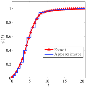
Fig. 12: The approximate cumulative spectral density associated with the modified 2D Laplacian constructed directly from a 20-step Lanczos run (left) and its spline-interpolated and smooth version (right).

Note that both $\psi(t)$ and $\widetilde{\psi}(t)$ are monotonically non-decreasing functions. Furthermore, it can been shown [26, 14] that $\psi(t)-\widetilde{\psi}(t)$ has precisely $2M-1$ sign changes within the spectrum of $A$. A sign change occurs when $\psi(t)$ crosses either a vertical or horizontal step of $\widetilde{\psi}(t)$. These properties allow us to construct an “interpolated” CDOS that matches $\psi(t)$ and $\widetilde{\psi}(t)$ at the points where $\psi(t)$ crosses $\widetilde{\psi}(t)$.

References

- [1] N. Ashcroft and N. Mermin, Solid State Physics, Thomson Learning, Toronto, 1976.
- [2] H. Avron and S. Toledo, Randomized algorithms for estimating the trace of an implicit symmetric positive semi-definite matrix, J. ACM, 58 (2011), p. 8.
- [3] S. R. Broderick and K. Rajan, Eigenvalue decomposition of spectral features in density of states curves, Europhysics Letters, 95 (2011), p. 57005.
- [4] F. W. Byron and R. W. Fuller, Mathematics of classical and quantum physics, Dover, New-York, 1992.
- [5] R. K. Chouhan, A. Alam, S. Ghosh, and A. Mookerjee, Ab initial study of phonon spectrum, entropy and lattice heat capacity of disordered Re-W alloys, Journal of Physics: Condense Matter, 24 (2012), p. 375401.
- [6] L. Covaci, F. M. Peeters, and M. Berciu, Efficient numerical approach to inhomogeneous superconductivity: The Chebyshev-Bogoliubov-de Gennes method, Phys. Rev. Lett., 105 (2010), p. 167006.
- [7] P. J. Davis, Interpolation and Approximation, Blaisdell, Waltham, MA, 1963.
- [8] T. A. Davis and Y. Hu, The University of Florida sparse matrix collection, ACM Trans. Math. Software, 38 (2011), p. 1.
- [9] Jos L. M. Van Dorsselaer, M. E. Hoschstenbach, and H. A. Van der Vorst, Computing probabilistic bounds for extreme eigenvalues of symmetric matrices with the lanczos method, SIAM J. Matrix Anal. Appl., 22 (2000), pp. 837–852.
- [10] David A. Drabold and Otto F. Sankey, Maximum entropy approach for linear scaling in the electronic structure problem, Phys. Rev. Lett., 70 (1993), pp. 3631–3634.
- [11] D. A. Drabold and O. F. Sankey, Maximum entropy approach for linear scaling in the electronic structure problem, Phys. Rev. Lett., 70 (1993), pp. 3631–3634.
- [12] F. Ducastelle and F. Cyrot-Lackmann, Moments developments and their application to the electronic charge distribution of d bands, J. Phys. Chem. Solids, 31 (1970), pp. 1295–1306.
- [13] A. Weiße, G. Wellein, A. Alvermann, and H. Fehske, The kernel polynomial method, Rev. Mod. Phys., 78 (2006), pp. 275–306.
- [14] B. Fischer and R. W. Freund, An inner product-free conjugate gradient-like algorithm for Hermitian positive definite systems, in Proceedings of the Cornelius Lanczos 1993 International Centenary Conference, 1994, pp. 288–290.
- [15] W. Gautschi, Computational aspects of three-term recurrence relations, SIAM Rev., 9 (1967), pp. 24–82.
- [16] , Construction of Gauss-Christoffel quadrature formulas, Math. Comp., 22 (1968), pp. 251–270.
- [17] , A survey of Gauss-Christoffel quadrature formulae, in E. B. Christoffel: The influence of his work in mathematics and the physical sciences, P. Butzer and F. Feher, eds., Basel, 1981, Birkhauser, pp. 72–147.
- [18] G. H. Golub and C. F. Van Loan, Matrix Computations, 4th edition, Johns Hopkins University Press, Baltimore, MD, 3rd ed., 2013.
- [19] G. H. Golub and J. H. Welsch, Calculation of Gauss quadrature rule, Math. Comp., 23 (1969), pp. 221–230.
- [20] R. Haydock, V. Heine, and M. J. Kelly, Electronic structure based on the local atomic environment for tight-binding bands, J. Phys. C: Solid State Phys., 5 (1972), p. 2845.
- [21] M. F. Hutchinson, A stochastic estimator of the trace of the influence matrix for Laplacian smoothing splines, Commun. Stat. Simul. Comput., 18 (1989), pp. 1059–1076.
- [22] D. Jackson, The theory of approximation, American Mathematical Society, New York, 1930.
- [23] L. O. Jay, H. Kim, Y. Saad, and J. R. Chelikowsky, Electronic structure calculations using plane wave codes without diagonlization, Comput. Phys. Comm., 118 (1999), pp. 21–30.
- [24] H. Jeffreys and B. Jeffreys, Methods of mathematical physics, Cambridge Univ. Pr., third ed., 1999.
- [25] D. Jung, G. Czycholl, and S. Kettemann, Finite size scaling of the typical density of states of disordered systems within the kernel polynomial method, Int. J. Mod. Phys. Conf. Ser., 11 (2012), p. 108.
- [26] S. Karlin and L. S. Shapley, Geometry of Moment Spaces, Amer. Math. Soc., 1953.
- [27] C. Lanczos, An iteration method for the solution of the eigenvalue problem of linear differential and integral operators, J. Res. Nat. Bur. Stand., 45 (1950), pp. 255–282.
- [28] , Applied analysis, Dover, New York, 1988.
- [29] N. N. Lebedev, Special functions and their applications, Dover, New York, 1972.
- [30] R. Li and Y. Zhou, Bounding the spectrum of large hermitian matrices, Linear Algebra and its Applications, 435 (2011), pp. 480–493.
- [31] W. Li, H. Sevincili, S. Roche, and G. Cuniberti, Efficient linear scaling method for computing the thermal conductivity of disordered materials, Phys. Rev. B, 83 (2011), p. 155416.
- [32] D. A. McQuarrie, Statistical Mechanics, Harper & Row, New York, NY, 1976.
- [33] G. A. Parker, W. Zhu, Y. Huang, D.K. Hoffman, and D. J. Kouri, Matrix pseudo-spectroscopy: iterative calculation of matrix eigenvalues and eigenvectors of large matrices using a polynomial expansion of the Dirac delta function, Comput. Phys. Commun., 96 (1996), pp. 27–35.
- [34] B. N. Parlett, The Symmetric Eigenvalue Problem, no. 20 in Classics in Applied Mathematics, SIAM, Philadelphia, 1998.
- [35] R. D. Richtmyer, Principles of advanced mathematical physics, vol. 1, Springer-Verlag, New York, 1981.
- [36] T. J. Rivlin, An introduction to the approximation of functions, Dover, New York, 2003.
- [37] L. Schwartz, Mathematics for the physical sciences, Dover, New York, 1966.
- [38] B. Seiser, D. G. Pettifor, and R. Drautz, Analytic bond-order potential expansion of recursion-based methods, Phys. Rev. B, 87 (2013), p. 094105.
- [39] R. N. Silver and H. Röder, Densities of states of mega-dimensional Hamiltonian matrices, Int. J. Mod. Phys. C, 5 (1994), pp. 735–753.
- [40] , Calculation of densities of states and spectral functions by Chebyshev recursion and maximum entropy, Phys. Rev. E, 56 (1997), p. 4822.
- [41] R. N. Silver, H. Röder, A. F. Voter, and J. D. Kress, Kernel polynomial approximations for densities of states and spectral functions, J. Comput. Phys., 124 (1996), pp. 115–130.
- [42] I. Turek, A maximum-entropy approach to the density of states within the recursion method, J. Phys. C, 21 (1988), p. 3251.
- [43] L.-W. Wang, Calculating the density of states and optical-absorption spectra of large quantum systems by the plane-wave moments method, Phys. Rev. B, 49 (1994), p. 10154.
- [44] John C. Wheeler and Carl Blumstein, Modified moments for harmonic solids, Phys. Rev. B, 6 (1972), pp. 4380–4382.
- [45] C. Yang, D. W. Noid, B. G. Sumpter, D. C. Sorensen, and R. E. Tuzun, An efficient algorithm for calculating the heat capacity of a large-scale molecular system, Macromol. Theory Simul., 10 (2001), pp. 756–761.
- [46] C. Yang, B. W. Peyton, D. W. Noid, B. G. Sumpter, and R. E. Tuzun, Large-scale normal coordinate analysis for molecular structures, SIAM J. Sci. Comp., 23 (2001), pp. 563–582.
- [47] Y. Zhou, Y. Saad, M. L. Tiago, and J. R. Chelikowsky, Parallel self-consistent-field calculations via Chebyshev-filtered subspace acceleration, Phy. Rev. E, 74 (2006), p. 066704.