Optical turbulence characterization at the SAAO Sutherland site

Abstract

We present results from the first year of a campaign to characterize and monitor the optical turbulence profile at the SAAO Sutherland observing station in South Africa. A MASS-DIMM (Multi Aperture Scintillation Sensor - Differential Image Motion Monitor) was commissioned in March 2010 to provide continuous monitoring of the seeing conditions. Over the first month of the campaign, a SLODAR (SLOpe Detection And Ranging) from Durham University was also installed allowing an independent verification of the performance of the MASS-DIMM device. After the first year of data collection, the overall median seeing value is found to be 1.32” as measured at ground level. The ground layer which includes all layers below 1 km accounts for 84% of the turbulence, while the free atmosphere above 1 km accounts for 16% with a median value of 0.41”. The median isoplanatic angle value is 1.92”, which is similar to other major astronomical sites. The median coherence time, calculated from corrected MASS measurements, is 2.85 ms. The seeing conditions at the site do show a strong correlation with wind direction with bad seeing conditions being associated with winds from the South-East.

1 Introduction

The degradation of astronomical image quality due to the distortion of light from atmospheric turbulence has been a long-known problem to astronomers (Tatarskii, 1961; Fried, 1966). Temperature and density gradients induce variations in the refractive index. As explained in Roddier (1981), the atmospheric turbulence arises from different layers in the atmosphere and is well describe by a Kolmogorov model. Turbulence is particularly evident in regions associated with wind shear between layers (Tatarskii, 1961). The strength of the turbulence in the different layers is commonly characterized by the index of refraction structure constant ($C_{N}^{2}(h)$), which is dependent on the altitude, $h$. Parameters used to characterize the optical turbulence depend on the cumulative effect from the turbulence from all layers in the atmosphere and can be calculated by integrating the $C_{N}^{2}$ profile along the path. These parameters include the coherence length or Fried Parameter ($r_{0}$), the coherence time ($\tau_{0}$), and the isoplanatic angle ($\theta_{0}$). In terms of image quality, the astronomical seeing ($\epsilon_{0}$), assuming a Kolmogorov turbulence model (ie. an infinite outer scale), is generally defined as the full width at half maximum (FWHM) of a long exposure image point spread function (PSF) and is inversely proportional to the Fried parameter such that FWHM = 0.98$\lambda/r_{0}$(Roddier, 1981).

Over the last 20 years, atmospheric site characterization and seeing monitoring for all major astronomical observatories has come into common usage (Els et al., 2009; Chun et al., 2009; Vernin & Munoz-Tunon, 1994). Indeed, seeing quality is one of the main critical parameter for site selection (IAU Symposium no.19, 1962; Coulman, 1985). In addition, continuous monitoring of the seeing is critical for optimizing observing schedules, especially for queue-scheduled observations (Sarazin, 1997). With the advent of adaptive optics (AO) systems (Babcock, 1953; Rigaut, 1992), one can now compensate for the image distortion due to atmospheric turbulence. Such systems rely on determining the turbulence properties of a site, and extensive characterization of the atmospheric turbulence are necessary.

The Sutherland observing station of the South African Astronomical Observatory (SAAO) was first quantitatively characterized in 1992 from photographic seeing measurements, and then later, these were supplemented by DIMM measurements from 1994 to 2000 (Erasmus, 2000; Gochermann et al., 1999). Since then, very little has been done in terms of optical site quality studies. In 2010, we initiated a comprehensive site characterization campaign to improve the scheduling of the Southern African Large Telescope (SALT) observations and provide the basis for a feasibility study of an AO system for the SALT.

In this paper we present the first year of seeing data. In §2, the main features of the site along with results from previous studies are presented. The Sutherland site monitoring instrument setup, data processing and analysis, and observing periods for the present study are described in §3. We describe the data analysis method and discuss data consistency in §4. The results are presented in §5 and discussed in §6. Finally, we conclude by summarizing the main results and future objectives for the Sutherland site characterization.

2 The SAAO Sutherland site

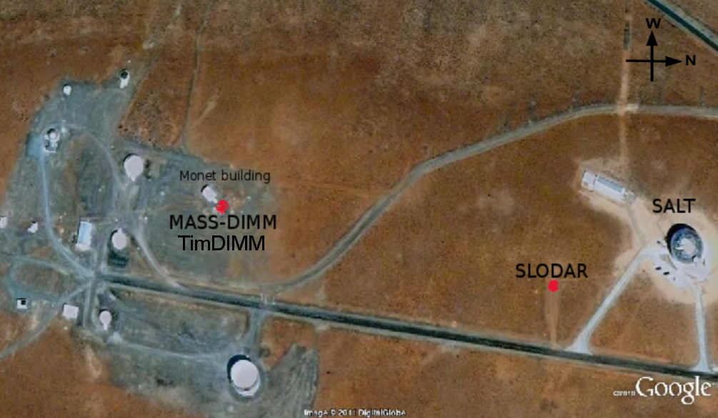
Figure 1: Sutherland site and the seeing monitoring instruments location

2.1 Location

The Sutherland site, located 370 km North-East of Cape Town in the semi-arid Karoo region, was founded in 1972 by merging the Republic Observatory (Johannesburg) and the Radcliffe Observatory (Pretoria) with the Royal Observatory (Cape of Good Hope). It is at 32^o23’ S latitude and 29^o49’ E longitude. The Sutherland plateau, host of 12 optical and infrared telescopes, has an altitude of 1768 m above sea level.

2.2 Historical site characterization results

The first historical report of seeing conditions at Sutherland was made by Harding (1974) and indicated 69% of the nights had seeing better than 0.8” from visual observations. Seeing measurements by Warner (1994), also based on eye measurements made during slit-scanning photometry of double stars observations between 1972 and 1994, reported 53% of the nights had seeing better than 0.8”. Due to the methodology used, it is difficult to evaluate the reliability of these measurements to compare to later quantitative results given by dedicated seeing monitors.

Seeing measurements were carried out using a trailed photographic technique from February 1992 to May 1993 by Gochermann et al. (1999). These results gave a median seeing of 1.23”, but were subject to wind effects.

Differential Image Motion Monitor (DIMM, Sarazin 1986a; Sarazin & Roddier 1990) observations were first obtained from April 1994 to February 1998. The system was based on that of Wood et al. (1995). These results were reported in Erasmus (2000) and indicated that the median seeing value for this period was 0.92” and the first and third quartiles were, respectively, 0.74” and 1.16” (Erasmus, 2000). A site testing campaign, using two DIMM instruments, was carried out to select the final site for SALT, from December 1998 to March 2000, and showed similar statistics with a median value of 0.95”, and first and third quartiles of 0.79” and 1.18” (Erasmus, 2000).

The seeing conditions measured over the period from April 1994 to February 1998 showed significant correlation with the wind speed and direction (Erasmus, 2000). South-Easterly winds brought poorer conditions while the best seeing value were observed for westerly winds. Also, worse seeing values tended to be associated with higher wind speed. The seeing conditions showed a very small dependence on the seasons. Observations during the SALT site testing campaign verified these correlations (Erasmus, 2000).

Considering the topography together with wind speed and directions at different altitudes, the main contributions to the turbulence were expected to be the surface layer up to 1 km, a wind shear layer around 3 km, and one between 10 and 12 km due to the jet stream (Erasmus, 2000). In addition, a 40 min scan from a classical SCIDAR (SCIntillation Detection And Ranging, Vernin & Roddier 1973) and microthermal measurements from a 30 m mast gave more information about the turbulence profile. The SCIDAR scan showed 3 strong layers at the ground level, around 3 km and 12 km. Based on the microthermal data, Erasmus (2000) found that the first 30 m of the ground layer (GL) were contributing only 7.3% of the overall turbulence with a seeing of 0.19”.

3 The Sutherland site monitoring setup

Over the past few decades several different methods have been developed to accurately measure atmospheric turbulence and turbulence profiles (TP). One of the more well-established methods combines a Multi Aperture Scintillation Sensor (MASS) and a Differential Image Motion Monitor (DIMM) into a single MASS-DIMM device (Kornilov et al., 2007). Such a device was installed and commissioned at the SAAO site in Sutherland in March 2010 with the objective of providing fully-automated, continuous seeing and turbulence profile measurements. During the year 2010 a SLOpe Detection And Ranging (SLODAR) instrument (Wilson, 2002) and a secondary DIMM instrument (hereafter referred to as TimDIMM) were also used alongside the MASS-DIMM. Eventually, in February 2011, the secondary DIMM operation stopped and its camera and operating procedure were transferred to the DIMM channel of the MASS-DIMM. The Sutherland instruments’ working principles, setup, operation and data processing are described in this section along with a summary of the observing periods for the different instruments reported in this paper.

The location of the different seeing instruments on the plateau can be seen on Fig. 1. The SLODAR was located in its own enclosure, while the MASS-DIMM and TimDIMM shared the same enclosure hereafter referred to as the DIMM building. Nightly seeing measurements from the MASS-DIMM are reported at http://www.salt.ac.za/$\sim$seeing.

3.1 SLODAR

3.1.1 Working principle

The SLODAR instrument is used to probe the ground layer (GL) profile of the atmospheric turbulence. The method uses a double star target to measure the spatial covariance of the slope of the wavefront phase aberration, seen at ground level, of two different paths through the atmosphere. In order to create two sets of spots, one for each star, the system uses a Shack-Hartmann wavefront sensor, mounted on a small aperture telescope. Using the spatial cross-covariance of the measured centroids, one can infer the turbulence profile (Butterley et al., 2006). The vertical resolution of the profiles depends on both the angular separation of the double star and its zenith distance. Aside from the GL profile, the SLODAR is also using the DIMM technique, described later, to determine the overall seeing value.

3.1.2 Location and general setup

The SLODAR was located approximately 100 m South-East from the SALT building. It uses a Schmidt-Cassegrain Meade telescope with a 40 cm aperture diameter mounted on an equatorial pier at ground level. The system was in a dome enclosure protected by a 2 m high wind screen.

3.1.3 Operation and control

The SLODAR was set up by two of us and operated from the University of Durham. The Sutherland setup uses a 8x8 Shack-Hartmann wavefront sensor with 5 cm size sub-apertures. With the system being fully robotic, it was operated from Durham, for the first 4 hours of the night, on each night when weather conditions allowed. More details on the operation and control are given in Wilson et al. (2009), which describes a similar setup of the instrument at Cerro Paranal. The higher vertical resolution of the Sutherland setup was achieved by using a CCD with a larger area that allowed a wider separation of the double stars. The resolution ranges from 55 to 80 meters, varying with star separation and elevation angle. Due to the wider separation, the maximum sensing altitude is around 500 m instead of 1km on a regular setup.

3.1.4 Data processing

The SLODAR data were processed as extensively detailed in Wilson et al. (2009). However the profile reconstruction model was modified and for the Sutherland data set is done using the ”Mk II” analysis mentioned in Wilson et al. (2011). The ”Mk II” analysis fits an extra turbulence component at the ground with a non-Kolmogorov power spectrum in order to account for dome/tube seeing. This component is also subtracted from the centroid autocovariance prior to fitting for r₀ to give an estimate of the total seeing that has been corrected for dome seeing.

3.2 TimDIMM

From July 2010 to January 2011 the TimDIMM was operated as a secondary DIMM instrument side by side with the MASS-DIMM. In February 2011, the CCD was migrated to the DIMM part of the MASS-DIMM to replace the SBIG-ST5, and the software was upgraded to handle the overall operation of the MASS-DIMM.

3.2.1 DIMM working principle

The DIMM is the most commonly used instrument for measuring the integrated seeing. The method is based on the differential motion of two images of a single star. The system uses a two aperture mask at the entrance pupil of the telescope with one aperture fitted with a thin-wedge prism to create two images of the same star, but with rays that propagate through different paths in the atmosphere. This way the stellar images share a common mount and optical system which greatly suppresses systematic errors due to telescope vibration and wind buffering. The DIMM principle is presented and discussed in Sarazin & Roddier (1990). The variance of the differential image motion is calculated from a series of images and the seeing is directly deduced via its relationship with the variance (Martin, 1987).

3.2.2 Location and general setup

The TimDIMM was located in the DIMM building next to the Monet-South telescope building, some 300 m South-East from the SALT. The system used a standard DIMM configuration (Sarazin & Roddier, 1990) on a 25 cm LX200-GPS Meade telescope mounted on the standard Meade tripod with an Alt-Az fork mount. The entrance aperture of the telescope lied at approximately 1.5 m from the ground. The detector used was a IEEE1394 camera from Point Grey Research (specifically, a Grasshopper GRAS-03K2M) which is capable of frame rates up to 200 Hz (full frame 640x480 pixels with no binning). A frame rate of 330 frames/sec with 2x2 binning is used in normal TimDIMM operations for additional speed and sensitivity.

3.2.3 Operation and control

The system’s pointing and tracking, as well as the real-time data analysis process are fully automated. The observing protocol is set so that the system selects targets with zenith angle less than 45^o and a magnitude less than 3. The system acquires 10000 frames to produce a seeing measurement. This provides a new seeing value every  30 seconds when running at the standard rate of 330 frames/sec and a 1 to 3 ms exposure time.

3.2.4 Data processing

The TimDIMM data are processed as described in detail in Tokovinin et al. (2002). The centroids of the stellar images are calculated via intensity-weighted moments within a 20x20 pixel box with a threshold set to 3$\sigma$ above the measured background noise in the image. Only pixels with signal above the threshold are included in the centroiding calculations. The weighted variance of the longitudinal differential motion is calculated using the signal-to-noise ratios as weights. We are not currently calculating the transverse variance, which is more sensitive to bias from wind smoothing (Kornilov & Safonov, 2011). The formal uncertainties in the centroids are used to determine the variance due to measurement uncertainty. This is then used to determine a corrected variance from which a seeing value is derived. We are also not applying an exposure time correction. With 1–3 ms exposures (depending on the star’s brightness) and a 3 ms cadence we have found it largely unnecessary.

3.3 MASS-DIMM

3.3.1 MASS working principle

The MASS instrument has been developed to provide a measurement of the free atmosphere (FA) seeing as well as a low resolution profile of the turbulence from 500m and above. Based on the well established relationship between scintillation from a single star image and atmospheric seeing (Roddier, 1981), it uses measurements of the scintillation in four concentric pupil apertures via photomultiplier tubes (PMTs) to recover the free atmosphere turbulence profile (Tokovinin et al., 2003b). The resolution and height of the measured C${}_{N}^{2}$ values are set by the diameter of the different apertures acting as spatial filters. Using both scintillation indices (SI) and differential scintillation indices (DSI), the MASS, with its current configuration, gives the C${}_{N}^{2}$ values at 0.5, 1, 2, 4, 8 and 16 km above the telescope. Moreover, the MASS also provides values for the coherence time and the isoplanatic angle. A full description of the device is given by (Kornilov et al., 2007).

3.3.2 MASS-DIMM configuration

The MASS-DIMM combines two instruments in a single device, as described in Kornilov et al. (2007). This requires some modifications to the instrument’s optical setup. Instead of an aperture mask at the telescope’s entrance pupil, an optical plate is positioned in the image pupil plane. This plate consists of two mirrors that form the two apertures of the DIMM channel and a pupil segmentor unit made of four concentric mirrors that feeds the MASS channel. An advantage of the MASS-DIMM is that it allows one to deduce the ground layer (GL) contribution to the turbulence by subtracting the free atmosphere (FA) seeing, given by the MASS channel, from the overall seeing measured by the DIMM channel (Tokovinin & Kornilov, 2007).

3.3.3 Location and general setup

The MASS-DIMM is located in the DIMM building next to the Monet-South telescope building, some 300 m South-East from the SALT. The system uses a 25 cm LX200GPS Meade telescope. From March 2010 to February 2011 it was mounted on the standard Meade tripod with an Alt-Az mount. Later, the mount was replaced by an Astro-Physics 900GTO equatorial mount and bolted directly to a steel pier. In both configurations the entrance aperture of the telescope lies between 1 and 1,5 m from the ground.

3.3.4 Operation and control

The MASS-DIMM in its first configuration (February 2010 to January 2011) was operated manually. The tracking was handled by the standard Meade Autostar II control system. The MASS data were handled by the Turbina 2.06 software (Kornilov et al., 2003). The DIMM imaging was done by an SBIG-ST5 CCD and the data were processed by the RoboDIMM software (Tokovinin et al., 2002). In January 2011, the alt-az mount was replaced by the equatorial one. From February 2011 onwards, the Point Grey IEEE1394 camera was migrated over from TimDIMM and replaced the ST5 on the MASS-DIMM. The TimDIMM software was updated to manage and control the entire MASS-DIMM system, including DIMM data acquisition and processing, handling telescope pointing and tracking, conducting the initialization and remote operation of the Turbina software and archiving of all seeing data.

Apart from roof opening, the MASS-DIMM has been working in fully robotic operation since March 2011. On all clear nights the system was operated by one of the SALT operators.

In summary, the current system is made up of a 25 cm telescope on an equatorial pier at ground level, the entrance aperture of the telescope being at approximately 1 m from the ground. Targets are automatically selected to have a magnitude lower than 3 and a zenith angle less than 45^o. The MASS data are processed by the Turbina 2.06 software , and the DIMM data are managed by the TimDIMM software, which also control the whole system. All of the data, raw and reprocessed, are stored within the SALT Science Archive.

3.3.5 Data processing

Prior to using the TimDIMM setup on the DIMM channel of the MASS-DIMM, the DIMM data were handled by the RoboDIMM software. A description of the latest version is given in Tokovinin et al. (2002), although we used a former version, Robodimmnet 1.4. In this configuration, the DIMM frame rate was set to 2 and 4 ms exposure time, allowing a correction of the finite exposure time to the zero exposure time, as described in Tokovinin (2002). The latest configuration uses the TimDIMM setup described in the previous section.

The MASS data are acquired by the Turbina software and reprocessed by the Atmos algorithm (Kornilov et al., 2002). The Atmos algorithm fits the measured SI and DSI to atmospheric models, assuming Kolmogorov turbulence, in order to restore the fixed and floating layers turbulence profile (Kornilov et al. (2002) 5.1.2.10). In this study we will use results from the fixed layers method which is tuned to give the C${}_{N}^{2}$ value at altitudes 0.5, 1, 2, 4, 8, and 16 km. Concerning the data acquisition, the PMTs have a 1 ms exposure time. Scintillation indices and statistical moments of the photon counts are calculated over a base-time of 1 sec, corresponding to hundred 1 ms samples. Those values are then averaged over a 1 min accumulation time, corresponding to 60 data point. After each accumulation time, atmospheric parameters are calculated from the SI, DSI and their respective errors, and then stored in the output file (Tokovinin et al., 2003b).

Previous studies of MASS and DIMM data quality indicate that data of low quality should be rejected (Kornilov et al., 2007; Wang et al., 2006). For DIMM data, the criteria are the number of frames per integration time (1 min) and the signal-to-noise ratio (SN) of the star images. For MASS data, we consider the flux in channel D, the error on the the flux measurement, the scintillation in channel A, and the $\chi^{2}$ of the restored profiles. A summary of the chosen threshold values is given in Table 1. We chose the threshold levels in agreement with those indicated in Kornilov et al. (2007), except for the flux level in channel D. The flux treshold accounts for clouds and target lost, Kornilov et al. (2007) indicates to choose a treshold of a minimum of 100 counts. However measurements with counts in chanel D as low as 50 are consistent with the rest of the data set from the same run. Hence, we choose to apply a treshold of 50 for the flux. The limit on the $\chi^{2}$ value allows to keep only data for which the reconstruction of the TP is accurate, and the threshold on the SI value suppresses data taken under strong scintillation for which the MASS measurements are not accurate (Tokovinin et al., 2003b). In order to be able to get a reliable value for the ground layer from differential DIMM and MASS measurements, we set the maximum value of $S_{A}^{2}$ to 0.7 as indicated in Kornilov et al. (2007). The percentage of data rejected for each thresholds never exceeds 5%, and the parameters values obtained from the raw data are within $\pm$ 6% of the ones obtained from the ”cleaned” data. For DIMM data, a flux threshold is also applied to each aperture along with a threshold on the number of frames used to calculate the variance of the differential image motion. This avoids biasing due to low signal-to-noise and helps to keep the statistics representative by maintaining a minimum number of samples per measurement.

Table 1: Data reprocessing thresholds

	Threshold parameter	Discrimination value
MASS	Flux in D channel	$>50$
	Flux error	$<0.01$
	$\chi^{2}$	$<100$
	$S_{A}^{2}$	$<0.7$
DIMM	Number of rejected frames	$<50$
	S/N	$>5$

Table 2: Observing periods with the Sutherland seeing monitoring instruments. The telescope diameter and DIMM operating and data processing softwares are given in parenthesis.

	SLODAR		MASS-DIMM						secondary DIMM
	(40 cm)		(25 cm)						(25 cm)
			MASS		DIMM (RoboDIMM)		DIMM (TimDIMM)		(TimDIMM)
Dates	$\#$ of nights	$\#$ of data	$\#$ of nights	$\#$ of data	$\#$ of nights	$\#$ of data	$\#$ of nights	$\#$ of data	$\#$ of nights	$\#$ of data
February 2010	8	1355	–	–	–	–	–	–	–	–
March 2010	16	2534	8	2108	8	2260	–	–	–	–
April 2010	4	646	20	7094	20	7817	–	–	–	–
May 2010	–	–	4	1180	4	1230	–	–	–	–
June 2010	–	–	1	–	1	–	–	–	–	–
July 2010	–	–	10	3983	7	2199	–	–	3	1272
August 2010	–	–	4	980	–	–	–	–	8	3990
September 2010	–	–	–	–	–	–	–	–	18	8436
October 2010	–	–	–	–	–	–	–	–	3	–
November 2010	–	–	1	239	–	–	–	–	14	7980
December 2010	–	–	2	614	–	–	–	–	14	2909
January 2011	–	–	16	4889	–	–	–	–	21	7500
February 2011	–	–	14	4277	–	–	14	7045	–	–
March 2011	–	–	11	3818	–	–	11	6001	–	–

3.4 Observing periods

This first year of seeing monitoring was conducted with several instruments that were operating at different periods, locations, and with different telescopes. Table 2 gives an overview of the different operation schedules for each instrument. Simultaneous operation of the SLODAR and MASS-DIMM were carried out over a period of 10 nights in March 2010. Also, from August 2010 to early January 2011, more DIMM than MASS data have been taken. This is due to the fact that the TimDIMM was set to be remotely controlled, while the MASS-DIMM still required manual operation. Only the TimDIMM was operated for most of the nights through this period. Data from June and October 2010 were included into the statistics for July and November respectively. Only few nights were observed during those months, and these nights were at the beginning or the end of the month.

4 Data analysis and consistancy

4.1 Data analysis method

For the purpose of data analysis, we define the free atmo- sphere (FA) as all layers above 1 km. We re-derive the FA seeing from the CN2 profile measured by the MASS consid- ering only the layers at and above 1 km and excluding the measurements at 500 m from MASS, which are known to be inaccurate (Tokovinin et al., 2005). However, the Atmos soft- ware, which computes the MASS atmospheric profile, uses triangular weighting functions to define the altitudes of the layers (Fig 2. in Tokovinin et al., 2003a). Due to the layer boundaries not being sharply defined, the reported CN2 value at a given altitude will include contributions from a range of heights. For example, the 1 km layer includes contributions from turbulence located between 500 m and 2 km. As such, any turbulence measured by MASS at a specific altitude is a weighted average of turbulence measured over the altitude range of the triangular weighting function. For simplicity in the rest of the paper, we will use 1 km as our boundary for the FA, but keeping in mind that this threshold is only approximate.

Defining the GL-FA boundary at 1 km requires a re-binning (in terms of altitude and time) of the data from the MASS-DIMM. The total integrated turbulence profile is given by:

$$J=\int_{0}^{\infty}C_{N}^{2}(h)dh.$$ (1)

The integrated turbulence profile can be given for different parts of the atmosphere by integrating $C_{N}^{2}(h)$ over different heights. For example, $J^{500}$ is given by integrating between 250 m and 1 km and using the triangular weighting function. $J^{MASS}$ is the sum of all layer contributions, $J^{500}+J^{1}+J^{2}+J^{4}+J^{8}+J^{16}$. The model gives a discrete representation of the turbulence which is in reality continuously distributed. If the real turbulence is at an altitude located in between two of the predefined layers altitude, it will be redistributed between those 2 adjacent layers through the triangular weighting functions (see fig. 6 and 7 in Tokovinin et al. (2003b)). It is shown in section 6.2 of Tokovinin et al. (2003b) that the redistribution induces errors on the individual layers contribution, reaching 20% in the worst cases for the lower 500 m and 1 km layers, but is typically between 5 to 10% for the overall contribution, $J^{MASS}$. The seeing in arcseconds for a given layer is just obtained through the following relation: $\epsilon=J^{3/5}\times 5.307\lambda^{-1/5}\times 206265$, where $\lambda$ is in $m$ and J is in $m^{1/3}$.

To determine the free atmosphere seeing, we must subtract the turbulence contribution of the 500 m layer from the overall MASS turbulence, then calculate the corresponding seeing. Using MASS profiles, the FA seeing ($\epsilon^{FA}$) is given by:

$$\epsilon^{FA}=[J^{MASS}-J^{500}]^{3/5}\times 5.307\lambda^{-1/5}\times 206265.$$ (2)

The GL seeing is then calculated as follow, after the 10 min binning:

$$\epsilon^{GL}=[(\epsilon^{DIMM})^{5/3}-(\epsilon^{FA})^{5/3}]^{3/5}.$$ (3)

In terms of qualitative analysis we will define best seeing conditions to be the first quartile of the seeing distribution, median conditions corresponds to the 25% around the median value, and bad conditions will be the fourth quartile of the seeing distribution.

4.2 Data consistency

4.2.1 MASS vs. DIMM

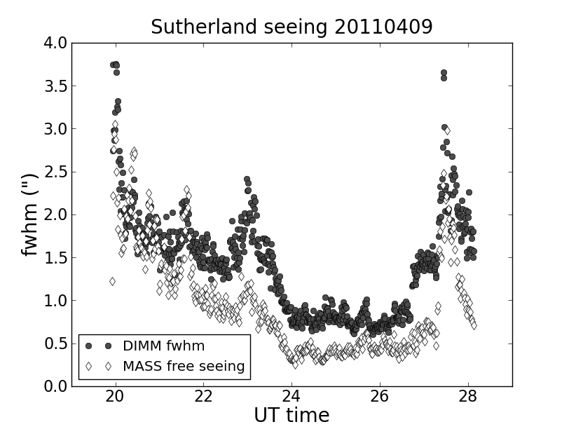
Figure 2: An example of the nightly variation of the overall seeing measured by DIMM (filled circle) and the seeing measured by MASS from layers above 500 m (open diamond).

Despite using two different technologies for measuring the seeing, the DIMM and the MASS show consistent behaviour throughout a typical night. An example of this is given in Fig.  2. As expected, $\epsilon^{DIMM}\geq\epsilon^{MASS}$, since the DIMM is measuring the overall seeing while the MASS is only measuring the FA seeing. However, on nights when the FA is dominant and one would expect $\epsilon^{MASS}\approx\epsilon^{DIMM}$, $\epsilon^{MASS}$ can be $>$ $\epsilon^{DIMM}$ due to the overestimation of the contribution of the lower layers to the MASS seeing (Tokovinin et al., 2005).

4.2.2 DIMM vs. SLODAR

As confirmation of the reliability of the seeing monitors, we compared seeing values as measured by the DIMM and the SLODAR. In order to do so, only data from overlapping observing periods have been considered. In addition, data have been binned and averaged over 10 minute periods to account for non-simultaneity of the measurements. The overall correlation between DIMM and SLODAR seeing values can be seen in Fig. 3. Each night is represented by a different data point and color. Despite a high dispersion on certain nights, the DIMM and SLODAR measurements are reasonably well correlated: the Pearson correlation coefficient, which measures linear relationships, is 0.69. A possible explanation for the differences between the instruments seen on any given night may be due to the different optical paths observed by each instrument as they were separated by 200 m on the plateau and were not always targeting the same star. In addition, the tendency of DIMM to give higher values can be explained by dome/tube seeing which, as mentioned in §3.1.4, has been removed from SLODAR measurements while it could still be affecting DIMM ones.

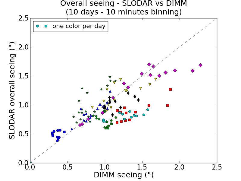
Figure 3: Comparison of the overall seeing value as measured by the DIMM and the SLODAR. Different data points and colors indicate different observing nights.

5 Results

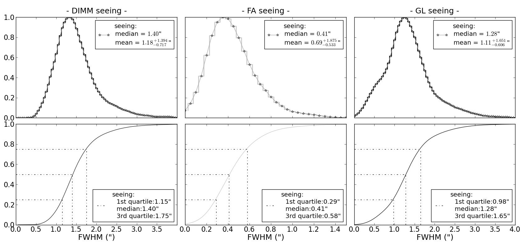
Figure 4: First year statistics of the seeing at the Sutherland site. Data from MASS-DIMM measurements, with the division between GL and FA defined to be at 1 km above ground level. All data have been averaged over 10 min. Left: Overall seeing as measured from DIMM. Center: Free-atmosphere seeing from MASS. Right: Ground-layer seeing derived from the difference between DIMM and MASS (see §4.1).

5.1 General statistics of the seeing

We used all of the DIMM data obtained with both MASS-DIMM (until July 2010) and TimDIMM (afterwards) with no temporal averaging to compute the median seeing for the site. The statistics for this present study are made of 53938 data points taken over a period of one year, from March 2010 to March 2011 and covering 146 nights. The median seeing value is 1.32”.

Using only the measurements for which both MASS and DIMM data are available, we looked at the contribution from the FA and the GL to the overall seeing. Distributions of the seeing values associated with each of these three components are shown in Fig. 4. To compare the MASS and DIMM measurements, we have averaged the data over 10 minute periods as explained in §4.1. Those results consist of 2564 data points observed over 91 days throughout the year, from March 2010 to March 2011. For this data set, the median overall seeing was 1.4” (Fig. 4, left), the median FA seeing was 0.41” (Fig. 4, middle) and the median GL seeing was 1.28” (Fig. 4, right).

5.2 Atmospheric turbulence profiles

5.2.1 Turbulence profiles from MASS-DIMM

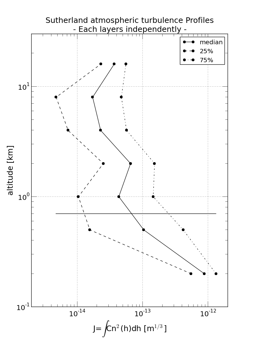
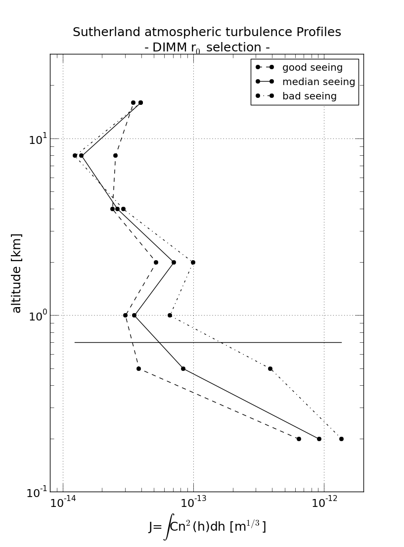
Figure 5: Turbulence profiles from MASS-DIMM: (a) gives the median (solid line), fisrt (dashed line) and third quartile (dotted line) value of the turbulence strength for each layer independantly, (b) represents the typical profiles under ”median” (solid line), ”good” (dashed line) and ”bad” (doted line) seeing conditions. ”Good”, ”median” and ”bad” are defined as the 20-30%, 45-55% and 70-80% ranges of the respective cumulative distribution of $\epsilon_{0}$.

Table 3: Contribution of the different layers for the median profile (solid line in Fig. 5-b)

	layer	layer contribution		seeing
	altitude	to the turbulence
	16 km	3.3%
	8 km	1.2%
FA	4 km	2.2%	15.7%	0.41”
	2 km	6%
	1 km	3%
	500 m	7%
GL			84.3%	1.28”
	200 m	77.3%
Overall				1.4”

In addition to the integrated parameters, the MASS-DIMM gives low resolution profiles of the turbulence. Fig.  5 shows the typical turbulence profiles at the Sutherland site. Fig. 5 (a) gives the median, first and third quartile value of the cumulative distribution of each layer independently. In Fig. 5 (b) we represent the profiles as selected by their associated $r_{0}$ value. ”Good” correspond to profiles for which the associated $r_{0}$ is within the 20-30% interval of its cumulative distribution. ”Median” correspond to the 45-55% interval and ”bad” is the 70-80% interval. The choice of interval was based on similar studies in the litterature (Els et al., 2009; Egner et al., 2007). The contribution of each layers in terms of $J$ value is represented for layers at different altitude. The FA layers are those given by the 1,2,4,8 and 16 km by the MASS. The GL has been divided into two layers: a 500 m layer also given by MASS and a 200m layer that includes all lower layers. The 200 m altitude was determined by taking the average altitude ($h_{eq}$) of the turbulence weighted by the turbulence strength at each altitude from SLODAR ground layer data, $h_{eq}=\frac{\sum h_{i}.J_{i}}{\sum J_{i}}$, which gives a value of 227 m.

Fig. 5 (a) only gives the median profile and the range of turbulence strength for each layer with the first and 3rd quartile values. While less representative of realistic profiles, due to the fact that it is unlikely to be in a configuration where all layers will be in their best condition or worse condition simultaneously, this representation is relevant for site comparison purpose.

Fig. 5 (b) is a more relevant plot in terms of site characterization as it gives the typical profiles corresponding to ”good”, ”bad”, and ”median” seeing conditions. One can see that, as the seeing degrades, the 200 m, 500 m, 1, and 2 km layers become more turbulent. While having a weaker contribution to the overall turbulence, the higher layers from 4 km and above remain, overall, fairly similar under all seeing conditions. However, the 8 km layer appears to be more turbulent under good seeing than for median and bad seeing. The overall contribution of the GL increases as the seeing degrades, being 80% under good seeing conditions (dashed line), 84% under median seeing (solid line) and nearly 88% under bad seeing (dotted line). Also, while the distribution between the two GL layers at 200 and 500 m does not change much between good and median seeing, it varies significantly under bad seeing conditions with 68% of the overall turbulence in the 200 m layer and 20% in the 500 m as compare to 77% and 7%, respectively, under median seeing. As the seeing degrades the 500 m layer contributes more to the GL turbulence. We will discuss this point further in the following section with the results of the GL profiles from SLODAR.

Overlall, based on the comparison of three typical profiles under good, median and bad seeing, one can conclude that the seeing value is mainly driven by the ground layer turbulence and to a weaker extent by the wind shear layer in the free atmosphere located around 2 km. The contribution from the different layers under median seeing conditions is summarized in Table 3.

5.2.2 Ground layer turbulence profiles from SLODAR

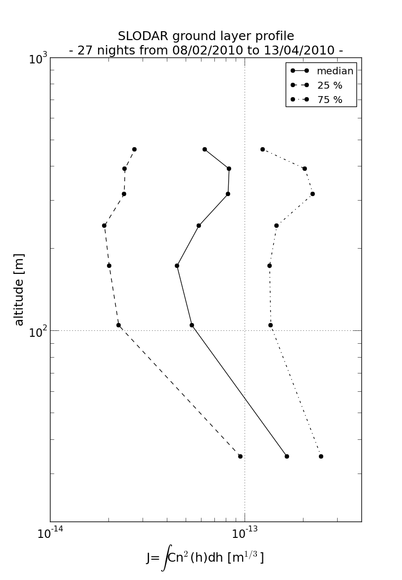
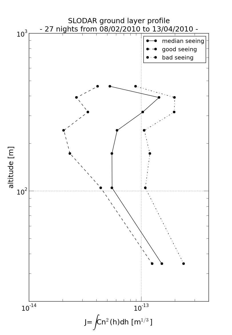
Figure 6: GL turbulence profiles from SLODAR, based on 27 nights of data between February and April 2010. (a) gives the median (solid line), fisrt (dashed line) and third quartile (dotted line) value of the turbulence strength for each layer independantly. (b) are the typical profiles under ”median” (solid line), ”good” (dashed line) and ”bad” (doted line) GL seeing conditions. ”median”, ”good” and ”bad” are defined as the 45-55%, 20-30% and 70-80% ranges of the cumulative distribution of $\epsilon_{0}^{GL}$.

Table 4: Contribution of the different layers for the GL median profile from SLODAR (solid line in Fig. 6-b)

layer altitude	layer contribution
35 m	24.5%
105 m	8.8%
173 m	8.8%
243 m	9.8%
318 m	16.6%
393 m	23.1%
462 m	8.4%

From the 27 nights of SLODAR measurements, we extracted the typical GL profiles. SLODAR profiles provide the turbulence strength for 7 layers whose altitudes vary slightly with both the separation and zenith angle of the target double star. For our typical profiles we determined each layer altitude by taking a weighted average, $h^{layer}=\frac{\sum h^{layer}_{i}.J^{layer}_{i}}{\sum J^{layer}_{i}}$, over all observations. Similarly to the profiles from MASS-DIMM we have represented the median, first and third quartiles for each layers independently on Fig. 6 (a), similar as to the measurements for Mauna Kea by Chun et al. (2009). Fig. 6 (b) shows the profiles correponding to ”good”, ”median” and ”bad” seeing condition with the same intervals as used for the MASS-DIMM profiles, but here using only the GL seeing value rather than the overall seeing. This method is similar to the measurements of Mount Graham by Masciadri et al. (2010).

Looking at the contribution from each layer for the profiles associated to the median seeing conditions (solid line in Fig. 6 (b) and summarized in Table  4), the first layer at 35 m contributes nearly 25% of the GL seeing while approximately 50% is contributed by layers above 300 m. On the other hand, under good seeing conditions nearly 40% of the turbulence is within the first 30 m while the upper layers are much weaker, particularly the 400 m that is now less than 10% of the turbulence. Under bad seeing the contribution of the lower 30 m goes down to 20% and the 300 to 500 m contribute around 45%, while the contribution from the intermediate layers, 100 to 300 m, increases to 30%. The degradation in the GL seeing corresponds to the increasing turbulence in the upper layers. This is in good agreement with our earlier observations from MASS-DIMM profiles which show an increase of the 500 m contribution as the seeing degrades.

In Section 6.2, we compare the profile of the GL at Sutherland with that measured at other sites.

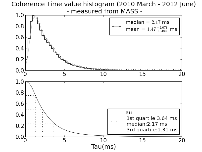
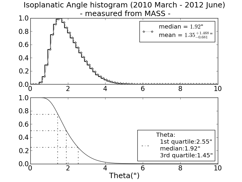
Figure 7: First year statistics of the seeing at the Sutherland site. MASS data. (a) Coherence time of the turbulence. (b) Isoplanatic angle.

5.3 Isoplanatic angle and coherence time

Table 5: Coherence time at Sutherland. Value given by the MASS instrument ($\tau_{0}^{MASS}$) and corrected value ($\tau_{0}^{corr}$). The correction uses $C=1.73$ and the GL contribution via $J_{GL}$ in equation (4). The wind speed was obtain from the weather mast data 30 m probe ($5.1m.s^{-1}$).

	median	25%	75%	$\epsilon_{0}$
				best 5%	best 20%
$\tau_{0}^{MASS}$ [ms]	2.17	3.64	1.31	8.87	4.33
$J_{GL}$ [$10^{-13}$ $m^{1/3}$]	8.99	5.88	14.02	0.32	4.92
(DIMM-MASS)
$\tau_{0}^{corr}$ [ms]	2.85	4.28	1.86	13.65	4.93
(MASS${}_{corr}+$GL)

In addition to the seeing value, the MASS also provides a measurement of both the coherence time ($\tau_{0}$) and the isoplanatic angle ($\theta_{0}$). Statistics of those two parameters are presented in fig.  7.

The median value of the coherence time ($\tau_{0}$) at Sutherland, as given from the MASS instrument, is 2.17 ms, the first and third quartile are respectively 3.64 and 1.31 ms. However it has been shown that the MASS measurement underestimates the coherence time (Tokovinin, 2006), but a correction can be applied. We will use equation (5) given in Tokovinin (2006):

$$\tau_{0}^{-5/3}=(C.\tau_{MASS})^{-5/3}+0.057^{-5/3}\lambda_{0}^{-2}V_{GL}^{5/3}J_{GL},$$ (4)

where $\tau_{MASS}$ is the value given by the MASS, $\lambda_{0}$ is the wavelength (500 nm), $V_{GL}$ is the ground layer wind speed obtained from the 30 m high probe on the weather mast ($5.1m.s^{-1}$ ) and $J_{GL}$ is the strength of the turbulence in the ground layer, derived from ${}^{\prime}DIMM-MASS^{\prime}$. $C$ is a correction coefficient, whose value is determined empirically with fairly low accuracy. Tokovinin found a value of 1.27, however he also mentioned a value of 1.7 and 1.73 found by Kornilov (2011) and Travouillon et al. (2009) as well as values varying between 2 and 2.5 found with comparative data at Cerro Tololo and Paranal. For the present study we will use $C=1.73$, given in Travouillon et al. (2009), as it is the most commonly used, and in particular for the TMT site testing. This gives us a consistent comparison between the Sutherland site and other sites around the world, keeping in mind that the accuracy of the method is $\pm$ 20%.

Results before and after applying the correction are presented in Table  5. After correction, the median value, first and third quartiles of the coherence time at Sutherland are respectively 2.85, 4.28 and 1.86 ms. We also looked at the coherence time value under good seeing conditions, for the $\epsilon_{0}$ best 5% and 20% values. We found, respectively, a 13.65 ms and 4.93 ms coherence time. Comparison values from 12 other sites are given in Table 6.

The isoplanatic angle median value at Sutherland is 1.92”. The values for 12 comparison sites are listed in Table 6. The first and third quartile values are respectively 2.55” and 1.45”, which gives a range of 1.1” between the best 25% and 75%. This is similar to all sites apart from Mauna Kea and Mount Graham spanning over a 2” range with best 25% of respectively 3.61” and 3.6” (TMT site selection team, 2008; Vázquez-Ramió et al., 2012).

5.4 Correlation of seeing with the weather conditions

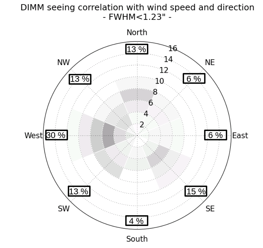
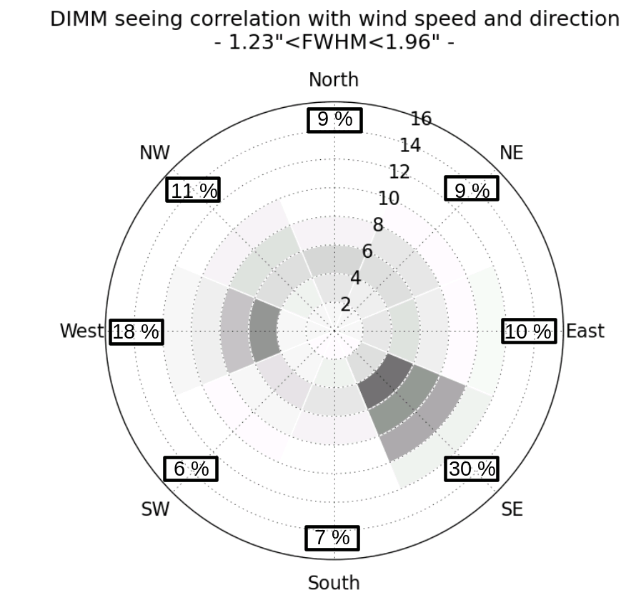
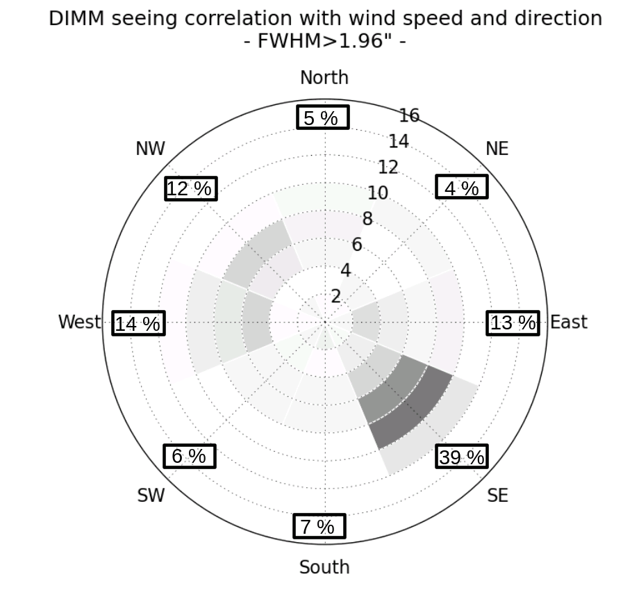
Figure 8: Correlation of seeing with wind direction and speed. In all three figures, the angle corresponds to the wind direction, the radius gives the wind speed in m/s, and the color gradient gives the density of data points. a) Good seeing conditions: $\epsilon_{0}\leq 1.23"$, corresponding to the first quartile. b) Median seeing conditions: $1.23"\leq\epsilon_{0}\leq 1.96"$. c) bad seeing conditions: $\epsilon_{0}\geq 1.96"$, corresponding to the third quartile. The percentages indicate the contribution of each wind directions in each wind rose.

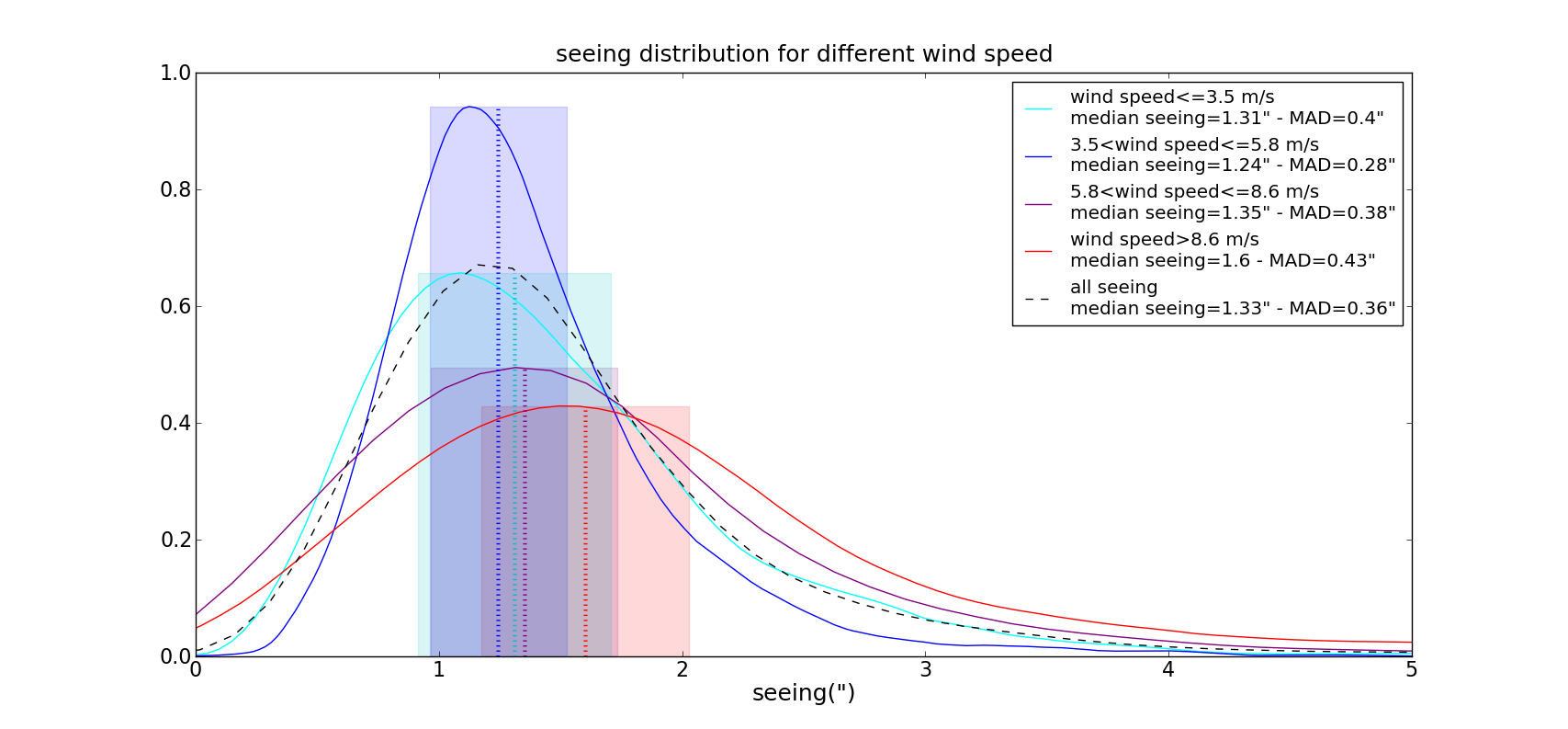
Figure 9: Relation between wind speed and seeing values. Dark blue: seeing distribution for lowest wind speed ($\leq$ 3.5 m/s). Light blue: seeing distribution for wind speed between 3.5 m/s and 5.8 m/s. Purple: seeing distribution for wind speed between 5.8 m/s and 8.6 m/s. Red: seeing distribution for highest wind speed ($\geq$8.6 m/s). The dashed line is plotted as an indicator and is the seeing distribution for all data. For all curves, the dotted line shows the median value and the shaded area corresponds to the median average deviation (MAD).

To see how the weather conditions influence the seeing, we compare our seeing measurements with data from the SALT weather station, which provided wind speed and direction at 10 and 30 m above ground, relative humidity level, and temperatures at 2,5,10,15,20,25,30 m above ground. Previous studies (Erasmus, 2000) showed that the wind was the main weather component influencing the seeing conditions. In examining the current weather data, we do find a strong correlation with wind direction, a weak correlation with wind speed, and we find no correlation with the temperature or relative humidity.

5.4.1 Influence of the wind direction

Fig. 8 presents the correlation of the seeing with wind speed and direction. We have plotted different cases corresponding to good seeing conditions (a), median seeing conditions (b), and bad seeing conditions (c). On the wind roses the angles indicate the wind direction and the radii the wind speed in m/s. After splitting the data according to their seeing value in the 3 different seeing conditions, we binned them within wind speed range of 2 m/s and wind directions range of 45^o. The color of each bin indicates the number of data within each bin, darker color indicating a higher number density of events. In addition, for each wind rose, we indicate the overall contribution of each wind direction in percentages of all data within each seeing range. Looking at Fig. 8 (a), one can see that good seeing occurred predominantly under westerly winds, while Fig. 8 (c) shows that bad seeing happened when winds were coming from the South-East. Apart from the North-West and North-East directions, having a fairly similar contribution under all seeing conditions, we could split the roses in two: the South-West to North half and the North-East to South half. If we look at the South-West to North half, the contribution from those wind directions gets weaker as the seeing degrades. On the other hand the North-East to South half direction contribute more and more with degrading seeing. It is clear here that as the wind turns West to South-East, the 2 predominant wind directions, the seeing degrades. Moreover, in the case of South-Easterly winds one can notice, by comparing the second and third roses, that the seeing tend to get worse with higher wind speed. However as we will see in the next section this is a behavior that is only visible in the case of South-Easterly winds.

5.4.2 Influence of the wind speed

The median seeing for 4 different wind speed ranges, corresponding to $<$3.5 m/s, 3.5 to 5.8 m/s, 5.8 to 8.6 m/s, and $>$8.6 m/s are presented in Fig. 9. The wind speed does not appear to have a very significant influence on the seeing, except at the highest wind speeds. However, the shift towards worse seeing for high wind speeds is not very pronounced, and may be due to telescope shake or higher dome seeing rather than higher atmospheric turbulence.

One could also suspect a wind speed bias due to the fact that the seeing monitors cannot operate at wind speed higher than 16 m/s. However winds above this speed were only recorded 2% of the time over the last three years. Moreover, the seeing value is only relevant within the conditions for which the telescopes are operational. Since the operation limit at Sutherland for the small telescopes and for normal operations of SALT is a wind speed limit of 16 m/s, we can neglect the effect of wind bias.

6 Discussion

6.1 Degradation in the Site Conditions

The value for the median seeing reported here is worse than those that were reported in earlier studies. Due to the methodology used in Warner (1994), we do not have a reliable way to compare their results with our study as discussed in §2.2. Concerning the site testing results from Erasmus (2000), a more reliable comparison is possible as those measurements were made using the same type of instrumentation. This previous campaign reported a median seeing of 0.92”, which is much lower than the 1.32” obtained from our entire set of DIMM data. That can be explained, to some extent, by the longer exposure time used in the previous study.

The bias in DIMM measurements due to long exposure times has been previously investigated by Tokovinin (2002). We can repeat that analysis for the specific observing setups used for DIMM measurements in Sutherland studies by stacking our exposures of 3.3 ms taken with TimDIMM. We estimate the bias in the DIMM measurements from Erasmus (2000) by replicating their 10 ms exposure time. The variance of the differential motion in the stacked image with a 9.9 ms exposure time was 0.62 times the variance of the differential motion in the individual 3.3 ms exposures. Applying this correction to the 0.92” seeing reported by Erasmus (2000) results in a seeing value of 1.25” for a 3.3 ms exposure time, which is not significantly different to our measured value of 1.32”. Although this result is similar to the analytic model of Tokovinin (2002) for the degradation of the seeing measurement, our estimate of the correction may be inaccurate due to difference in the conditions when the original observations were made. Regular, long-term monitoring with the same instrument is required to determine how the site might be changing and whether those changes could be related to climatic change in Sutherland as has been seen at other sites (Sarazin, 2010).

6.2 Site Comparison

Table 6: Comparison of Sutherland with other sites.

	altitude [m]	median seeing			$\theta_{0}$	$\tau_{0}$	# nights / # data
Site		overall	GL	FA		(MASScorr+GL)
Sutherland	1768	1.4”	1.28”	0.41”	1.92”	2.9 ms	91 / 29,182
March 2010 - March 2011
Cerro Tololo (Els et al., 2009)	2207	0.88”	0.44”	0.50”	1.56”	2.9 ms	NA / 433,162
2004-2008
Mauna Kea (Chun et al., 2009)	4050	0.71”	0.51”	0.42”	2.69”	5.1 ms	124 / NA
2006-2007
Paranal (Sarazin et al., 2008)	2635	1.1”	0.86”	0.56”	2.6”	3.6 ms	NA / NA
2007
Mount Graham (Masciadri et al., 2010)	3221	0.95”	0.81”	0.39”	2.5”	4.8 ms	43 / 16,659
2007
Cerro Las Campanas (Thomas-Osip et al., 2012)	2551	0.8”	0.58”†	0.47”	1.84”	2.46 ms‡	46 / 3,412
2010
E-ELT (Vázquez-Ramió et al., 2012)
2008-2009 ($\sim 1$ year per site)
Aklim (Morocco)	2350	1.0”	0.77”	0.52”	1.29”	3.5 ms	NA / 10,992
Cerro Maón (Argentina)	4653	0.87”	0.51”	0.66”	1.37”	3.4 ms	NA / 29,723
Roque de los Muchachos (Canary Island)	2346	0.8”	0.65”	0.32”	1.93”	5.6 ms	NA / 47,328
Cerro Ventarrones (Chile)	2837	0.91”	0.6”	0.55”	1.96”	4.9 ms	NA / 56,547
TMT (TMT site selection team, 2008)
2003-2008 ($>2.5$ years per site)
Cerro Tolar (Argentina)	2290	0,63”	0.34”	0.44”	1.93”	5.2 ms	NA / 196,812
Cerro Armazones (Chile)	3064	0.64”	0.35”	0.43”	2.04”	4.6 ms	NA / 212,367
Cerro Tolonchar (Chile)	4480	0.64”	0.32”	0.48”	1.83”	5.6 ms	NA / 89,958
San Pedro Mártir (Mexico)	2830	0.79”	0.58”	0.37”	2.03”	4.2 ms	NA / 139,359
$\dagger$GL seeing is not given in arcseconds in the reference paper, hence we calculated it from the MASS and DMM seeing values using the
following formulae: $see_{GL}=(see_{DIMM}^{5/3}-see_{MASS}^{5/3})^{3/5}$
$\ddagger$MASS time constant - not corrected

As reported in §5.1, the median integrated seeing conditions as measured for when both MASS and DIMM were operational and after a 10 minute binning was 1.4”. We use this value to provide a uniform comparison to other sites, in terms of overall, FA and GL seeing. This median seeing is worse than that reported at other major astronomical observatories (Table 6), including Paranal (Sarazin et al., 2008), Cerro Tololo (Els et al., 2009), Mauna Kea (Chun et al., 2009), Mount Graham (Masciadri et al., 2010), Las Campanas (Thomas-Osip et al., 2012) and both the sites tested for the E-ELT (Vázquez-Ramió et al., 2012) and TMT (TMT site selection team, 2008). However, the FA seeing is comparable to the best astronomical sites (Table 6), which confirms the fact that turbulence at Sutherland is dominated by the ground layer. In terms of the other atmospheric parameters, the median isoplanatic angle at Sutherland, 1.92”, is very similar to most sites. Five of the sites have a smaller isoplanatic angle, between 1.29” and 1.84”, 3 have comparable values between 1.93” and 1.96” and 5 have larger values between 2.03” and 2.69” (see §5.3 for details). Despite long coherence time under good seeing conditions, 13.7 ms for the best 5% and 4.9 ms for the best 10%, the median coherence time of 2.7 ms for Sutherland is significantly shorter than at other sites that have values between 3.4 ms and 5.6 ms. As seen in equation (4) the GL component of the coherence time is larger under weak turbulence (represented by $J_{GL}$). The overall coherence time combines both the FA and GL coherence time, but we have seen that the FA turbulence component is very similar between sites, hence the coherence time is highly influenced by the strong turbulence of the ground layer at Sutherland compare to other sites. However this dependence is also due the method used to derive the coherence time from MASS-DIMM data. The accuracy of the coefficient $C$ in equation (4) is questionable. Comparing $\tau_{0}$ results from MASS and DIMM measurements also shows discrepancies. Previous results from M. Sarazin at Paranal , reported in Tokovinin (2006), show that $\tau_{0}^{DIMM}$, calculated from equation (3) in Sarazin et al. (2008), gives values 2.5 larger than $\tau_{0}^{MASS}$. Here the correction we applied gives $\tau_{0}\sim 1.31\tau_{0}^{MASS}$, which might still be underestimating the actual value. Considering the discrepancy between measurements from MASS and other instruments, as well as the low reliability of the correction applied due to the wide range of value for the coefficient $C$ found in the literature, more investigation on the $\tau_{0}$ value is needed.

The observed overall worse seeing conditions at Sutherland compared to other sites can be partly explained due to several discrepancies between our data set and those from other sites results. First, many of these sites have only fully published results from earlier periods and we are not comparing results over the same time period. Recent results from Paranal indicated the seeing conditions have degraded over the last decade and that this may be due to longer term climatic changes (Sarazin, 2010).

Another important caveat is that the DIMMs at the comparison sites are typically located on 5 m high towers, while the Sutherland DIMM is located at ground level. Hence, our results may be strongly affected by convective turbulence from the ground. Using the results from MASS-DIMM, SLODAR profiles, and previous studies, we can estimate the effect due to the lower 5 m surface layer. From MASS-DIMM, we found that 84% of the turbulence is located in the GL, and the SLODAR results tell us that the lowest 30 m contributed 25% of the GL. In Erasmus (2000), it is reported that the first 5 m have a seeing of 0.15”, which correspond to 66.3% of the turbulence associated to the 0.19” seeing of the first 30 m for that period. Using the same proportion we can reasonably consider that the first 5 m contributes roughly 14% of the overall turbulence. From this, we would expect that the integrated median seeing measured from a 5 m platform would be 1.28”. Following the same procedure, the expected seeing at the dome entrance for SALT, which is located at approximately 30 m, would be 1.22”. In addition, when fitting the dome/tube seeing for profile reconstruction in SLODAR, part of the turbulence outside the dome belonging to the ground layer might be subtracted resulting in an underestimation of both the ground layer and the overall turbulence. As a result the first 30 m may be contributing more than 25% of the turbulence.
However, despite the facts considered above, the altitude of the Sutherland site (1768 m) is much lower than all the other sites whith altitudes ranging from 2290 m to 4653 m, so we do not expect the seeing at Sutherland to be as good as these other sites.

In terms of GL, both Chun et al. (2009) and Masciadri et al. (2010), respectively for Mauna Kea and Mount Graham, presented high vertical resolution turbulence profiles. The Sutherland site differs signifcantly from those two sites due to its strong upper ground layer located at 300 to 500 m. The Sutherland upper GL contributes nearly 50% of the GL turbulence while it is only 2% and 12% for Mauna Kea and Mount Graham, respectively. Most of the turbulence at those sites is located in the lower layers, 90% in the first 40 m for Mauna Kea and 70% in the first 100 m for Mount Graham, compare to 30% in the first 100 m at Sutherland.

6.3 Weather conditions bias

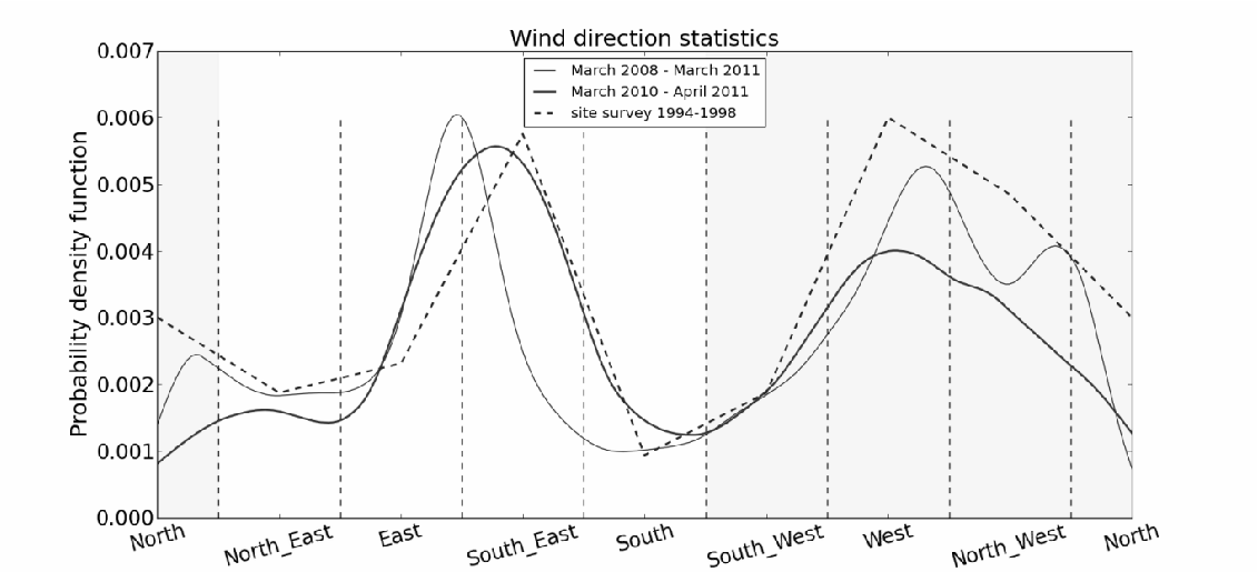
Figure 10: Wind direction and seeing. Wind direction frequencies during our seeing measurements (thick line) compare to those of the past 3 years (thin line) and those of the site testing campaign (Erasmus, 2000) (dashed line). The x axis indicates the wind directions. The shaded area correspond to wind directions associated with good seeing.

In order to comment on potential bias of our data set due to weather conditions during our observing period, we used weather data from the SALT weather station taken between April 2008 and April 2011 and consisting of 966 nights and 729663 data points. A comparison between the wind directions during this period and our site monitoring campaign indicates that the typical seeing at Sutherland is expected to be lower than the results presented here. For the following discussion we will use all DIMM measurements without any averaging.

Comparing the occurrence of the wind directions during our site survey campaign with three years of weather data (presented in Fig.  10), one would expect the seeing to be slightly better over this three year period as conditions associated with good seeing (winds from the westerly direction) are more prevalent than during our site monitoring campaign. Indeed, during our campaign, winds associated with bad seeing correspond to 39.4% of our data while those associated with good seeing correspond to 49.2%. In comparison, the long term weather data indicate winds associated to bad seeing occur only 28.3% of the time, while those associated to good seeing represent 58.4% of the data. Moreover, the wind pattern for the past three years is in very good agreement with that reported in Erasmus (2000) (dashed line in Fig. 10), which showed good seeing conditions 57% of the time and bad seeing conditions 29.4% of the time.

If we use the past three years as representing the typical wind pattern, we can estimate the median seeing conditions for Sutherland based on the distribution of wind direction and the correlation between the seeing and wind direction presented in §5.4.1. Using these values and the three year wind direction data, we expect the median seeing to be around 1.2” as compared to that measured for the year 2010-2011, including all DIMM data without any averaging, of 1.32”.

7 Conclusions

While previous studies of the Sutherland site provided a good general overview of the observing conditions, they were lacking the turbulence profile and did not reflect the current conditions. Hence the present study provides an up-to-date view of the Sutherland site seeing conditions. In addition, it also provides a detailed monitoring of the atmospheric turbulent profile, albeit only over one year.

This first year of seeing monitoring resulted in the successful installation of a fully automated MASS-DIMM providing continuous seeing monitoring for all observers on the plateau at Sutherland. With a year of seeing measurements consisting of 27 days of SLODAR operations, 91 days of MASS-DIMM data, and 55 additional days of TimDIMM measurements, we obtained the first atmospheric turbulence measurements at the Sutherland site.

The median seeing for the Sutherland site from these data is 1.4”. Like most astronomical sites, Sutherland has 3 main layers contributing to the turbulence: the GL below 1 km, a layer in which turbulence is driven by the wind shear whose altitude varies between 2 and 5 km, and finally the upper layers above 12 km where turbulence are associated to the jet-stream. Under median conditions, the GL contributes 84% of the turbulence of the integrated seeing. Moreover, we know from SLODAR profiles that the GL is dominated by the first 30 m and the higher 300 to 500 m.

With this instrumentation in place and a future upgrade with a 5 m tower, long-term monitoring of the site will allow further investigation of any seasonal bias to atmospheric conditions, as well as longer timescale climatic effect, e.g. associated with El Niño/La Niña. The availability of real-time seeing data, along with the behaviour of the atmospheric conditions, will allow for improved observing planning efficiencies, especially at SALT, which is a queue scheduled telescope. The preponderance of the GL turbulence is promising for the development of a ground layer adaptive optics systems for the Sutherland telescopes, and future campaigns with additional site testing equipment will refine the turbulence profile measured here, as well as the coherence time value.

8 Acknowledgements

This work is based upon research supported by the National Research Foundation (NRF) and the UK Science & Technology Facilities Council.
The authors are thankful to the referee for the valuable and constructive comments and suggestions given. We also wish to thank the SALT Foundation, who funded and own the seeing instruments, as well as the SAAO and SALT operations staff for the logistical support in this study.

References

- Babcock (1953) Babcock, 1953, PASP, 65, 229
- Butterley et al. (2006) Butterley T., Wilson R., Sarazin M., 2006, MNRAS, 369, 835
- Chun et al. (2009) Chun M. et al., 2009, MNRAS, 394, 1121
- Coulman (1985) Coulman C.E., 1985, ARA&A, 23, 19
- Egner et al. (2007) Egner S.E. et al., 2007, PASP, 119, 669
- Els et al. (2009) Els S.G. et al., 2009, PASP, 121, 922
- Erasmus (2000) Erasmus A., 2000, Sth. Af. J. Sci., 96, 475
- Fried (1966) Fried D.L., 1966, PASP, 56, 1372
- Gochermann et al. (1999) Gochermann J. et al., 1999, Exp. Ast., 9, 1
- Harding (1974) Harding G. A., 1974, SAAOC, Vol. 1 - P. 31
- Kornilov et al. (2002) Kornilov V., Potanin S., Shatsky N., Voziakova O., Zaitsev A. 2002, MASS Software Reference Manual - Part II - data processing
- Kornilov et al. (2003) Kornilov V., Shatsky N., Vaziakova O., 2003, MASS Software Version 2.04 User Guide
- Kornilov et al. (2007) Kornilov V., Tokovinin A., Shatsky N.,Voziakova O., Potanin S. F., Safonov B., 2007, MNRAS, 382, 1268
- Kornilov & Safonov (2011) Kornilov V. and Safonov B., 2011, MNRAS, 418, 1878
- Kornilov (2011) Kornilov V., 2011, A&A, 530, A56
- Masciadri et al. (2010) Masciadri E., Stoesz J., Hagelin S., Lascaux F., 2010, MNRAS, 404, 144
- Martin (1987) Martin H. M., 1987, PASP, 99:1360-1370
- Rigaut (1992) Rigaut F., 1992, Univ. de Paris, Rigaut F.
- Roddier (1981) Roddier F., 1981, Prog. Optics, 19, 281
- IAU Symposium no.19 (1962) Rosch J., 1962, IAU Symposium no.19, Gauthier-Villars, Paris
- Sarazin (1986a) Sarazin M., 1986a, SPIE Conf. S., 628, 138
- Sarazin & Roddier (1990) Sarazin M., Roddier F., 1990, A&A, 227, 294
- Sarazin (1997) Sarazin M., 1997, Proc. SPIE, 3125, 366
- Sarazin & Tokovinin (2002) Sarazin M., Tokovinin A., 2002, ESO Con. and Work. proc., 58, 231
- Sarazin et al. (2008) Sarazin M., Melnick J., Navarrete J., Lombardi G., 2008, The Messenger, 132, 11
-
Sarazin (2010)
Sarazin M., 2010 - http:www.eso.org/gen-fac/pubs/astclim
/papers/review00/seeing3.html - Tatarskii (1961) Tatarski V. I., 1961, Dover Publications, Inc., New York
- TMT site selection team (2008) TMT site selection team, 2008, TMT site testing final report, TMT.SIT.TEC.08.2003.REL01
- Tokovinin et al. (2002) Tokovinin A., Bustos E., Schwarz H., 2002, CTIO RoboDIMM v2.3 software description
- Tokovinin (2002) Tokovinin A., 2002, PASP, 114, 1156
- Tokovinin et al. (2003a) Tokovinin A., Baumont S, Vasquez J., 2003a, MNRAS, 340, 52
- Tokovinin et al. (2003b) Tokovinin A., Kornilov V., Shatsky N.,Voziakova O., 2003b, MNRAS, 343, 891
- Tokovinin et al. (2005) Tokovinin A., Vernin J., Ziad A., Chun M., 2005, PASP, 117:395-400
- Tokovinin (2006) Tokovinin A., 2006, ”Calibration of the MASS time constant measurements”. Internal report - http://www.ctio.noao.edu/ atokovin/profiler/timeconst.pdf
- Tokovinin & Kornilov (2007) Tokovinin A., Kornilov V., 2007, MNRAS, 381, 1179
- Thomas-Osip et al. (2012) Thomas-Osip J. E. et al., 2012, PASP, 124, 84
- Vázquez-Ramió et al. (2012) Vázquez-Ramió et al., 2012, PASP, 124, 868
- Travouillon et al. (2009) Travouillon T., Els S., Riddle R. L., Schöck M., Skidmore W., 2009, PASP, 121, 787
- Vernin & Roddier (1973) Vernin J., Roddier F., 1973, JOSA, 63, 270
- Vernin & Munoz-Tunon (1994) Vernin J., Munoz-Tunon C., 1994, A&A, 284, 311
- Wang et al. (2006) Wang et al., 2006, SPIE, 6267, 62671S
- Warner (1994) Warner B., 1994, MNSSA, 53, 46
- Wilson (2002) Wilson R., 2002, MNRAS, 337, 103
- Wilson et al. (2009) Wilson R., Butterley T., Sarazin M., 2009, MNRAS, 399, 2129-2138
- Wilson et al. (2011) Wilson R., Butterley T., Osborn J. and Shepherd H., 2011, ”Optical turbulence profiling and applications for astronomy,” in Signal Recovery and Synthesis, OSA Technical Digest (CD) (Optical Society of America, 2011), paper JTuA1.
- Wood et al. (1995) Wood P.R., Rodgers A.W. and Russell K.S. , 1995, PASA, 12, 97-105