Differentiating the production mechanisms of the Higgs-like resonance using inclusive observables at hadron colliders

Abstract

We present a study on differentiating direct production mechanisms of the newly discovered Higgs-like boson at the LHC based on several inclusive observables. The ratios introduced reveal the parton constituents or initial state radiations involved in the production mechanisms, and are directly sensitive to fractions of contributions from different channels. We select three benchmark models, including the SM Higgs boson, to illustrate how the theoretical predictions of the above ratios are different for the $gg$, $b\bar{b}(c\bar{c})$, and $q\bar{q}$ (flavor universal) initial states in the direct production. We study implications of current Tevatron and LHC measurements. We also show expectations from further LHC measurements with high luminosities.

Keywrords: Higgs Physics, Beyond Standard Model

I Introduction

Recently, a new resonance with a mass around 126 GeV has been discovered by the ATLAS Aad:2012tfa and CMS Chatrchyan:2012ufa . It is considered to be a highly Standard Model (SM) Higgs-like particle with measured production rate consistent with the SM Higgs boson through $\gamma\gamma$, $ZZ^{*}$, $WW^{*}$, and $\tau\tau$ channels Aad:2012tfa ; Chatrchyan:2012ufa . Although further efforts are required in order to determine the features of the new resonance, like the spin, couplings with SM particles, and self-couplings. The spin-1 hypothesis is excluded by the observation of the $\gamma\gamma$ decay mode according to the Landau-Yang theorem Landau:1948kw ; Yang:1950rg . Many proposals have been suggested to distinguish between the spin-0 and spin-2 hypotheses mainly focusing on the kinematic distributions, e.g, angular distributions Choi:2002jk ; Gao:2010qx ; DeRujula:2010ys ; Englert:2010ud ; Ellis:2012wg ; Bolognesi:2012mm ; Choi:2012yg ; Ellis:2012jv ; Englert:2012xt ; Banerjee:2012ez ; Modak:2013sb ; Boer:2013fca ; Frank:2013gca , event shapes Englert:2013opa and other observables Boughezal:2012tz ; Ellis:2012xd ; Alves:2012fb ; Geng:2012hy ; Djouadi:2013yb . Recent measurements ATLAS:2013xla ; ATLAS:2013mla ; Aad:2013xqa ; CMS:xwa show a favor of spin-0 over specific spin-2 scenarios. As for the couplings, the current direct information or constraints are for the relative strength between different observed channels, i.e., $\gamma\gamma$, $ZZ^{*}$, $WW^{*}$, and $\tau\tau$ Aad:2012tfa ; Chatrchyan:2012ufa . Without knowing the total decay width and rates from other unobserved channels it is difficult to determine the absolute strength of the couplings of the new resonance at the LHC. Or later we can further measure the couplings through a combined analysis after the observation of the associated production modes with the SM $W$ and $Z$ bosons or the vector-boson fusion (VBF) production mode Plehn:2001nj ; Giardino:2012ww ; Rauch:2012wa ; Azatov:2012rd ; Low:2012rj ; Carmi:2012in ; Plehn:2012iz ; Djouadi:2012rh .

Among all the couplings of the new resonance, the ones with gluons or quarks are important but difficult to be measured at the LHC since the corresponding decay modes consist of two jets, which suffer from huge QCD backgrounds at the LHC even for the heavy-quark (charm or bottom quark) jets. Moreover, it is extremely hard to discriminate the couplings with gluons and light-quarks from the resonance decay. This relates to the answer to a more essential question, i.e., the direct production of the new resonance is dominated by the gluon fusion or quark annihilation. In the SM, the loop-induced gluon fusion is dominant while the heavy-quark annihilation only contributes at a percent level. As for other hypotheses, like in the two Higgs doublet models, the heavy-quark contributions can be largely enhanced Djouadi:2005gj ; Meng:2012uj , or in the graviton-like cases ArkaniHamed:1998rs ; Randall:1999ee , the light-quark contributions are important as well.

Similar as in the determination of the spin of the new resonance, we can use the angular distributions of the observed decay products, like $\gamma\gamma$, $ZZ^{*}$, and $WW^{*}$, to differentiate the $gg$ and $q\bar{q}$ production mechanisms as in ATLAS:2013xla ; ATLAS:2013mla ; Aad:2013xqa ; CMS:xwa . But the analyses are highly model-dependent, i.e., the angular distributions are sensitive to the spin of the resonance as well as the structures of the couplings with the decay products Gao:2010qx . On another hand, since these two production mechanisms depend on different flavor constituents of the parton distribution functions (PDFs), they may show distinguishable behaviors by looking at the ratios of the event rate at different colliders or center-of-mass energies as previously shown in Mangano:2012mh for various SM processes at the LHC including for the SM Higgs boson, or the rapidity distribution of the resonance. Even more ambitious, we may look at the production of the resonance in association with an additional photon or jet from initial state radiations which are presumably to be different for the gluon and quark initial states. Unlike the case of the angular distributions, all these observables are insensitive to details of couplings with the decay products. Thus they may serve as good discriminators of the direct production mechanisms of the new resonance.

Based on the above ideas we present a study of using inclusive observables to discriminate the mechanisms of the direct production of the new resonance, including both the theoretical predictions and the experimental feasibilities. In Section II, we describe the benchmark models of the production mechanisms studied in this paper, and introduce several inclusive observables that are used in our study. Section III compares the theoretical predictions of the observables from different models. In Section IV we discuss the applications on current experimental data from the Tevatron and LHC, and also future measurements at the LHC. Section V is a brief conclusion.

II Model setups and inclusive observables

We select three benchmark models in the study, including the pure SM case, an alternative spin-0 resonance with enhanced couplings to the charm and bottom quarks, and a spin-2 resonance with universal couplings to all the quarks. As explained in the introduction, our analyses mainly rely on the fractions of the $gg$ and $q\bar{q}$ contributions in the production mechanism and are insensitive to details of couplings with the decay products. More precisely, the relevant effective couplings for the spin-0 cases are given by

$${\mathcal{L}}_{spin-0}={g_{1}^{(0)}\over v}HG^{\mu\nu}G_{\mu\nu}+{g_{2}^{(0)}\over v}(m_{c}H\bar{\Psi}_{c}\Psi_{c}+m_{b}H\bar{\Psi}_{b}\Psi_{b}),$$ (1)

and for the spin-2 case by Englert:2012xt

$${\mathcal{L}}_{spin-2}=g_{1}^{(2)}Y_{\mu\nu}T_{G}^{\mu\nu}+g_{2}^{(2)}Y_{\mu\nu}T_{q}^{\mu\nu},$$ (2)

with $H$ being the scalar particle, $Y_{\mu\nu}$ the general spin-2 fields spin2a ; spin2b , $G_{\mu\nu}$ the field strength of QCD, and $\Psi_{c,b}$ the charm and bottom quarks. We choose graviton-inspired couplings for the spin-2 case with $T_{G}^{\mu\nu}$ and $T_{q}^{\mu\nu}$ being the energy-momentum tensors of the gluon and quarks (flavor universal) as can be found in Hagiwara:2008jb . Here we suppress all other couplings of the resonance with the $W$, $Z$ bosons, photon, and $\tau$ lepton, which are adjusted to satisfy the corresponding decay branching ratios observed Aad:2012tfa ; Chatrchyan:2012ufa , especially the couplings with photons should be suppressed in order to be consistent with the experimental measurements. We work under an effective Lagrangian approach and will not discuss about the possible UV completion of the theory.

For model A, the pure SM, we have

$$v=246\,{\rm GeV},\,\,g_{1}^{(0)}={\alpha_{s}\over 12\pi},\,\,g_{2}^{(0)}=1,\,\,m_{c(b)}=0.634(2.79)\,{\rm GeV},$$ (3)

where $g_{1}^{(0)}$ are evaluated at the LO in the infinite top quark mass limit, and the heavy-quark masses are $\overline{\rm MS}$ running mass at the resonance mass $m_{X}=126\,{\rm GeV}$ Beringer:1900zz ; Chetyrkin:2000yt . From a phenomenological point of view, we introduce model B, the heavy-quark dominant case with $g_{1}^{(0)}=0$. Note that $g_{1}^{(0)}$ always receives non-zero contributions from the heavy-quark loops proportional to $g_{2}^{(0)}$. However, in global analyses of the Higgs couplings Carmi:2012in ; Djouadi:2012rh , it is always treated as another free parameter that could in principle vanish, since its actual value depends on details of the underlying new physics. Thus model B is a phenomenological simplification of models with heavy-quark annihilation dominant in the production, e.g., supersymmetric models with large $\tan\beta$ Djouadi:2005gj . The absolute value of $g_{2}^{(0)}$ is irrelevant for the study here. Similar for model C, the spin-2 case, we set $g_{1}^{(2)}=0$ with the production dominated by the light quarks. It is shown that a spin-2 model with minimal couplings Gao:2010qx to the vector bosons has been ruled out by both the ATLAS and CMS despite of the production mechanism Aad:2013xqa ; CMS:xwa . The measurements utilize angular distributions of final states from decay vector bosons. As shown in Gao:2010qx , these angular distributions are sensitive to detailed structures of the couplings to the vector bosons. Thus the exclusion could not be applied to a general spin-2 model involving much more free parameters in the vector boson couplings Gao:2010qx . In contrast the observables introduced below are independent of the couplings to the decay vector bosons.

The inclusive observables we studied can be divided into three categories. First one is the ratio of the inclusive cross sections of the direct production, $R^{1}$, including the cross sections at the Tevatron, and at the LHC with different center-of-mass energies. The second one is the ratio of the direct production cross sections in the inner and full rapidity region of the produced resonance, $R^{2}$. These two observables probe the production mechanisms through the differences of the relevant PDFs. The third observable, $R^{3}$, is the ratio of the production cross section of the resonance in association with a photon to the one of the direct production. It differentiates the production channels by measuring the initial state radiations. For the calculation of $R^{3}$ we neglect the small explicit couplings of the new resonance with photons in the production. Other observables that might be sensitive to the production mechanisms are related to the initial state QCD radiations, like the $p_{T}$ spectrum or jet-bin cross sections Dittmaier:2012vm ; Wiesemann:2012ij of the resonance, which are again different for the $gg$ and $q\bar{q}$ initial states. But that will be even more challenging in both the theory predictions and experimental measurements.

III Benchmark comparisons

III.1 Ratios of the total cross section

Here we calculate the total cross sections of the direct production of the new resonance at the Tevatron and LHC with $\sqrt{s}=7$, 8, and 14 TeV. At the leading order (LO), they are related to the following parton-parton luminosities,

$$L_{gg}(\tau)=\int_{\tau}^{1}\frac{dx_{1}}{x_{1}}\int_{\tau/x_{1}}^{1}\frac{dx_{2}}{x_{2}}\tau^{2}f_{g/h_{1}}(x_{1},\mu_{f})f_{g/h_{2}}(x_{2},\mu_{f})\delta(x_{1}x_{2}-\tau),$$

$$L_{c\bar{c}(b\bar{b})}(\tau)=\int_{\tau}^{1}\frac{dx_{1}}{x_{1}}\int_{\tau/x_{1}}^{1}\frac{dx_{2}}{x_{2}}\tau^{2}[f_{c(b)/h_{1}}(x_{1},\mu_{f})f_{\bar{c}(\bar{b})/h_{2}}(x_{2},\mu_{f})+h_{1}\leftrightarrow h_{2}]\delta(x_{1}x_{2}-\tau),$$

$$L_{q\bar{q}}(\tau)=\sum_{q}\int^{1}_{\tau}\frac{dx_{1}}{x_{1}}\int^{1}_{\tau/x_{1}}\frac{dx_{2}}{x_{2}}\tau^{2}[f_{q/h_{1}}(x_{1},\mu_{f})f_{\bar{q}/h_{2}}(x_{2},\mu_{f})+h_{1}\leftrightarrow h_{2}]\delta(x_{1}x_{2}-\tau),$$ (4)

where $\tau=m_{X}^{2}/s$, $x_{1,2}$ are the momentum fractions. $\mu_{f}$ is the factorization scale and set to $m_{X}$ in our calculations. $f_{i/h}(x)$ are the PDFs, and the sum in $L_{q\bar{q}}$ runs over all the 5 active quark flavors. Thus the typical Bjorken $x\sim m_{X}/\sqrt{s}$ are about 0.06, 0.018, 0.016, and 0.009 at the Tevatron, LHC 7, 8, and 14 TeV. While beyond LO, there are also contributions from other flavor combinations subject to different $x_{1}-x_{2}$ constraints. We select 5 ratios from all the cross sections, $R^{1}_{L7/T}=\sigma({\rm LHC}\,7\,{\rm TeV})/\sigma({\rm Tevatron})$, similar for $R^{1}_{L8/T}$, $R^{1}_{L14/T}$, $R^{1}_{L14/L7}$, and $R^{1}_{L14/L8}$. The cross sections for models A and B can be calculated up to next-to-next-to-leading order (NNLO) in QCD using the numerical code iHixs1.3 Anastasiou:2011pi . While it is only calculated at the LO for the model C. Note that the ratios $R^{1}$ at the LO are totally determined by the behaviors of the parton-parton luminosities in Eq. (III.1) and are independent of the detailed structures of the couplings, while at higher orders they may show slight dependence on the couplings. We set the renormalization scale to $m_{X}=126\,{\rm GeV}$ as well, and use the most recent NNLO PDFs including CT10 Gao:2013xoa , MSTW 2008 Martin:2009iq , and NNPDF2.3 Ball:2012cx . The PDF and $\alpha_{s}$ uncertainties are calculated and combined using the prescription in Ball:2012wy .

In Table. 1 we show the predicted ratios $R^{1}$ for the SM Higgs boson from different PDF groups. It can be seen that the current uptodate NNLO PDFs give pretty close results for the ratios. The combined PDF+$\alpha_{s}$ uncertainties are about 7% for the ratios of the NNLO cross sections at the LHC over Tevatron due to the relatively large uncertainties of the gluon PDF at the large $x$ region. While the uncertainties are reduced to a level of about 2% for the ratios at the LHC. Theoretical uncertainties due to the missing higher order QCD corrections can be estimated by looking at the differences of the results at different orders, which are smaller compared to the combined PDF+$\alpha_{s}$ uncertainties and are not considered in our analysis. Tables. 2 and 3 show similar results for the model B and C. The heavy quark PDFs are mostly generated through the evolution of the gluon PDF. Thus the results of the model B are close to the SM case. The model C predicts very different results compared to the SM or model B, for the ratios of the NNLO cross sections at the LHC over Tevatron, and also shows smaller uncertainties, since the cross sections are dominated by the light quark scattering.

model A	CT10			MSTW08			NNPDF2.3			Combined
	LO	NLO	NNLO	LO	NLO	NNLO	LO	NLO	NNLO	NNLO
$R^{1}_{L7/T}$	$17.9^{+0.8}_{-1.0}$	$17.5^{+0.8}_{-0.9}$	$17.0^{+0.7}_{-0.9}$	$18.1^{+0.5}_{-0.5}$	$17.7^{+0.5}_{-0.5}$	$17.2^{+0.5}_{-0.5}$	$18.6^{+0.6}_{-0.6}$	$18.1^{+0.6}_{-0.5}$	$17.5^{+0.5}_{-0.5}$	$17.1^{+1.1}_{-1.1}$
$R^{1}_{L8/T}$	$22.9^{+1.1}_{-1.3}$	$22.4^{+1.0}_{-1.2}$	$21.7^{+1.0}_{-1.2}$	$23.2^{+0.7}_{-0.7}$	$22.6^{+0.7}_{-0.7}$	$21.9^{+0.7}_{-0.7}$	$23.9^{+0.8}_{-0.8}$	$23.2^{+0.7}_{-0.7}$	$22.4^{+0.7}_{-0.7}$	$21.8^{+1.5}_{-1.5}$
$R^{1}_{L14/T}$	$59.9^{+3.4}_{-4.1}$	$58.5^{+3.1}_{-3.8}$	$56.3^{+3.0}_{-3.6}$	$60.7^{+2.3}_{-2.2}$	$59.3^{+2.2}_{-2.1}$	$57.0^{+2.1}_{-2.0}$	$62.2^{+2.4}_{-2.3}$	$60.6^{+2.2}_{-2.1}$	$58.1^{+2.1}_{-2.0}$	$56.6^{+4.3}_{-4.3}$
$R^{1}_{L14/L7}$	$3.34^{+0.04}_{-0.05}$	$3.35^{+0.04}_{-0.05}$	$3.32^{+0.04}_{-0.05}$	$3.35^{+0.03}_{-0.03}$	$3.35^{+0.03}_{-0.03}$	$3.32^{+0.03}_{-0.03}$	$3.34^{+0.03}_{-0.03}$	$3.34^{+0.03}_{-0.02}$	$3.31^{+0.02}_{-0.02}$	$3.31^{+0.05}_{-0.05}$
$R^{1}_{L14/L8}$	$2.61^{+0.02}_{-0.03}$	$2.62^{+0.02}_{-0.03}$	$2.60^{+0.02}_{-0.03}$	$2.62^{+0.02}_{-0.02}$	$2.62^{+0.02}_{-0.02}$	$2.60^{+0.02}_{-0.02}$	$2.61^{+0.02}_{-0.02}$	$2.61^{+0.02}_{-0.01}$	$2.59^{+0.01}_{-0.01}$	$2.59^{+0.03}_{-0.03}$

Table 1: Predicted ratios $R^{1}$ at different orders from various PDFs with the PDF+$\alpha_{s}$ uncertainties at 68% C.L. for the case of pure SM.

model B	CT10			MSTW08			NNPDF2.3			Combined
	LO	NLO	NNLO	LO	NLO	NNLO	LO	NLO	NNLO	NNLO
$R^{1}_{L7/T}$	$23.0^{+1.5}_{-1.8}$	$22.7^{+1.6}_{-1.9}$	$23.4^{+1.7}_{-2.0}$	$23.5^{+1.0}_{-1.0}$	$23.2^{+1.1}_{-1.1}$	$24.0^{+1.2}_{-1.2}$	$24.6^{+1.2}_{-1.2}$	$24.4^{+1.3}_{-1.2}$	$25.3^{+1.5}_{-1.4}$	$24.2^{+3.2}_{-3.2}$
$R^{1}_{L8/T}$	$29.8^{+2.1}_{-2.5}$	$29.4^{+2.2}_{-2.6}$	$30.4^{+2.4}_{-2.8}$	$30.5^{+1.4}_{-1.4}$	$30.0^{+1.5}_{-1.5}$	$31.2^{+1.7}_{-1.7}$	$32.0^{+1.7}_{-1.6}$	$31.6^{+1.8}_{-1.7}$	$33.0^{+2.0}_{-1.9}$	$31.4^{+4.3}_{-4.3}$
$R^{1}_{L14/T}$	$81.2^{+6.6}_{-7.8}$	$79.4^{+6.8}_{-7.9}$	$82.8^{+7.5}_{-8.6}$	$83.1^{+4.7}_{-4.6}$	$81.6^{+5.0}_{-4.8}$	$85.3^{+5.6}_{-5.4}$	$87.4^{+5.2}_{-4.9}$	$85.8^{+5.5}_{-5.1}$	$90.0^{+6.2}_{-5.7}$	$85.6^{+13.1}_{-13.1}$
$R^{1}_{L14/L7}$	$3.53^{+0.06}_{-0.07}$	$3.50^{+0.06}_{-0.07}$	$3.54^{+0.06}_{-0.08}$	$3.54^{+0.04}_{-0.04}$	$3.52^{+0.04}_{-0.04}$	$3.55^{+0.05}_{-0.04}$	$3.54^{+0.04}_{-0.04}$	$3.52^{+0.04}_{-0.04}$	$3.55^{+0.04}_{-0.04}$	$3.53^{+0.09}_{-0.09}$
$R^{1}_{L14/L8}$	$2.72^{+0.03}_{-0.04}$	$2.70^{+0.04}_{-0.04}$	$2.72^{+0.04}_{-0.04}$	$2.73^{+0.02}_{-0.02}$	$2.71^{+0.03}_{-0.02}$	$2.73^{+0.03}_{-0.03}$	$2.73^{+0.02}_{-0.02}$	$2.71^{+0.02}_{-0.02}$	$2.73^{+0.02}_{-0.02}$	$2.72^{+0.05}_{-0.05}$

Table 2: Predicted ratios $R^{1}$ at different orders from various PDFs with the PDF+$\alpha_{s}$ uncertainties at 68% C.L. for model B.

model C	CT10	MSTW08	NNPDF2.3	Combined
	LO	LO	LO	LO
$R^{1}_{L7/T}$	$3.96^{+0.07}_{-0.06}$	$4.00^{+0.04}_{-0.06}$	$3.95^{+0.06}_{-0.05}$	$3.98^{+0.10}_{-0.10}$
$R^{1}_{L8/T}$	$4.68^{+0.08}_{-0.08}$	$4.72^{+0.05}_{-0.07}$	$4.67^{+0.07}_{-0.06}$	$4.70^{+0.12}_{-0.12}$
$R^{1}_{L14/T}$	$9.17^{+0.20}_{-0.20}$	$9.19^{+0.13}_{-0.16}$	$9.10^{+0.14}_{-0.12}$	$9.18^{+0.25}_{-0.25}$
$R^{1}_{L14/L7}$	$2.32^{+0.02}_{-0.02}$	$2.30^{+0.01}_{-0.01}$	$2.30^{+0.01}_{-0.01}$	$2.31^{+0.02}_{-0.02}$
$R^{1}_{L14/L8}$	$1.96^{+0.01}_{-0.01}$	$1.94^{+0.01}_{-0.01}$	$1.95^{+0.01}_{-0.01}$	$1.96^{+0.02}_{-0.02}$

Table 3: Predicted ratios $R^{1}$ at the LO from various PDFs with the PDF+$\alpha_{s}$ uncertainties at 68% C.L. for model C.

III.2 Centrality ratio

At the LO, the rapidity of the produced resonance in the lab frame is given by, $y=\ln(x_{1}/x_{2})/2$, or equivalently $y=\ln((1+\beta)/(1-\beta))/2$, where $\beta$ is the boost of the resonance. We define the centrality $R^{2}$ as the ratio of the production cross section in the central region (with $|y|<1$) to the one in the full rapidity region, which are related to the corresponding ratio of the parton-parton luminosities at the LO, $L(\tau,|y|<1)/L(\tau)$. For illustration purpose, we show the above luminosity ratio as functions of the rapidity cutoff in Fig. 1 for different parton combinations shown in Eq. (III.1).

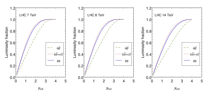
Figure 1: Luminosity fractions as a function of the rapidity cutoff at the LHC with different center-of-mass energies.

The calculated centrality ratios for the models A, B, and C are listed in Tables. 4-6 for different PDFs at the LHC. Again for the pure SM case, the predictions are at the NNLO in QCD from HNNLO1.3 code Catani:2007vq . Others are only calculated at the LO. Here we simply choose the central region of $|y|<1$ for the definition of $R^{2}$. In principle one can find the optimized value that gives largest distinctions of the three models. Similar to the case of $R^{1}$, the models A and B give close results of $R^{2}$ but with larger uncertainties compared to $R^{1}$. The differences of the predictions from the model C with the ones from the model A or B are still significant.

model A	CT10			MSTW08			NNPDF2.3			Combined
	LO	NLO	NNLO	LO	NLO	NNLO	LO	NLO	NNLO	NNLO
$R^{2}_{L7}$	$0.536^{+0.009}_{-0.013}$	$0.536^{+0.009}_{-0.013}$	$0.533^{+0.009}_{-0.013}$	$0.538^{+0.005}_{-0.007}$	$0.537^{+0.005}_{-0.007}$	$0.538^{+0.005}_{-0.007}$	$0.548^{+0.008}_{-0.008}$	$0.546^{+0.008}_{-0.008}$	$0.547^{+0.008}_{-0.008}$	$0.539^{+0.018}_{-0.018}$
$R^{2}_{L8}$	$0.518^{+0.009}_{-0.012}$	$0.519^{+0.009}_{-0.012}$	$0.526^{+0.009}_{-0.012}$	$0.518^{+0.009}_{-0.003}$	$0.522^{+0.009}_{-0.003}$	$0.532^{+0.009}_{-0.003}$	$0.529^{+0.008}_{-0.008}$	$0.530^{+0.008}_{-0.008}$	$0.538^{+0.008}_{-0.008}$	$0.531^{+0.017}_{-0.017}$
$R^{2}_{L14}$	$0.453^{+0.007}_{-0.008}$	$0.453^{+0.007}_{-0.008}$	$0.450^{+0.007}_{-0.008}$	$0.454^{+0.004}_{-0.004}$	$0.454^{+0.004}_{-0.004}$	$0.452^{+0.004}_{-0.004}$	$0.461^{+0.005}_{-0.005}$	$0.460^{+0.005}_{-0.005}$	$0.458^{+0.005}_{-0.005}$	$0.453^{+0.012}_{-0.012}$

Table 4: Predicted ratios $R^{2}$ at different orders from various PDFs with the PDF+$\alpha_{s}$ uncertainties at 68% C.L. for the case of pure SM.

model B	CT10	MSTW08	NNPDF2.3	Combined
	LO	LO	LO	LO
$R^{2}_{L7}$	$0.575^{+0.012}_{-0.017}$	$0.578^{+0.006}_{-0.008}$	$0.592^{+0.010}_{-0.010}$	$0.580^{+0.023}_{-0.023}$
$R^{2}_{L8}$	$0.555^{+0.012}_{-0.015}$	$0.556^{+0.014}_{-0.004}$	$0.571^{+0.010}_{-0.010}$	$0.561^{+0.022}_{-0.022}$
$R^{2}_{L14}$	$0.487^{+0.009}_{-0.011}$	$0.489^{+0.005}_{-0.006}$	$0.498^{+0.007}_{-0.007}$	$0.490^{+0.016}_{-0.016}$

Table 5: Predicted ratios $R^{2}$ at the LO from various PDFs with the PDF+$\alpha_{s}$ uncertainties at 68% C.L. for model B.

model C	CT10	MSTW08	NNPDF2.3	Combined
	LO	LO	LO	LO
$R^{2}_{L7}$	$0.364^{+0.004}_{-0.005}$	$0.358^{+0.005}_{-0.002}$	$0.361^{+0.002}_{-0.002}$	$0.362^{+0.007}_{-0.007}$
$R^{2}_{L8}$	$0.351^{+0.004}_{-0.005}$	$0.345^{+0.002}_{-0.003}$	$0.348^{+0.002}_{-0.002}$	$0.349^{+0.008}_{-0.008}$
$R^{2}_{L14}$	$0.309^{+0.004}_{-0.005}$	$0.303^{+0.002}_{-0.003}$	$0.309^{+0.002}_{-0.002}$	$0.306^{+0.007}_{-0.007}$

Table 6: Predicted ratios $R^{2}$ at the LO from various PDFs with the PDF+$\alpha_{s}$ uncertainties at 68% C.L. for model C.

III.3 Associated production

Here we consider the ratios of the cross sections for the resonance production in association with a photon to the ones of the direct production, $R^{3}\equiv\sigma_{X+\gamma}/\sigma_{X}$. The advantage is that for the case of the SM, this associated production mode is largely suppressed with main contributions from the $b\bar{b}$ annihilation at the LHC Abbasabadi:1997zr . While for models B and C, the associated production is only suppressed by the QED couplings even though the statistics are low at the LHC. The calculations for the associated production are performed at the LO. Thus, for consistency we use the LO cross sections of the direct production as well. Moreover, for the model C, we apply a form factor Frank:2013gca

$$F=\left(\frac{\Lambda^{2}}{\hat{s}+\Lambda^{2}}\right)^{5},$$ (5)

to the associated production by multiplying it with the squared amplitudes since the effective operator there violates unitarity above a certain energy scale. Here $\hat{s}$ is the square of the partonic center-of-mass energy, and we choose the cutoff scale $\Lambda$ to be $800\,{\rm GeV}$. We select the events from the associated production with a rapidity cut of $|y_{\gamma}|<2$ and a transverse momentum cut $p_{T,\gamma}>15\,{\rm GeV}$ on the photon. Here we adopt a relatively lower $p_{T}$ cut on the photon in order to maximize the statistics of the associated production. Fig. 2 shows ratios of the cross sections of associated production to the ones of the direct production as functions of the $p_{T}$ cut of the photon at the LHC with different center-of-mass energies. It can be seen that for the SM case, the cross sections of the associated production are negligible, less then $10^{-4}$ times the cross sections of the direct production. While for models B and C the ratios are larger by an order of magnitude comparing to the SM, and the associated production may be observable at the LHC. For lower $p_{T}$ cutoff the ratios from models B and C are close. At moderate or high $p_{T}$ cutoff the ratios from model C are larger due to the power enhancement from high dimension operators, and are sensitive to the form factor applied and the UV completion of the theory. The central values and the PDF+$\alpha_{s}$ uncertainties of $R^{3}$ predicted in different models are listed in Tables. 7-9.

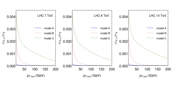
Figure 2: Ratios of the cross sections of the associated production to the ones of the direct production as functions of the $p_{T}$ cut of the photon, at the LHC with different center-of-mass energies.

We may also utilize production of the resonance in association with a jet, and study the effects on observables like jet-bin (jet-veto) fractions, $p_{T}$ distribution of the resonance as recently measured in TheATLAScollaboration:2013eia . The cross sections of associated production with a jet are much larger compared to the case of a photon due to the strong couplings as well as opening of new partonic channels. Especially for the SM case, $gg$ channel now contributes and dominates over all others. Similarly, we consider a ratio of the one-jet inclusive cross sections to the total inclusive ones, $\sigma_{X+jet}/\sigma_{X}$. For example, using both LO cross sections, we obtain the ratio as 0.355 (0.128) for model A (B) at the LHC 8 TeV. Here we require a jet to have $|y|<2$ and $p_{T}>30\,{\rm GeV}$. We can see the ratio is larger for the SM case, in contrary with the case of a photon, because of the stronger radiations from gluon initial states and the high dimension effective operators. Thus this ratio may have some discrimination powers on different production mechanisms. At the same time it also has larger theoretical and experimental uncertainties associated with the jet. The resummed $p_{T}$ spectrums of the resonance produced through $gg$ and $b\bar{b}$ initial states have been predicted in Glosser:2002gm ; Bozzi:2003jy ; Field:2004tt and Field:2004nc ; Belyaev:2005bs respectively. Shapes of the two distributions are very similar with both peak located around $10\sim 20$ GeV at the LHC for a resonance mass of about 120 GeV. Note that experimentally the jet may fake a photon with a rate depending on both the kinematics and photon isolation criteria. For the SM case, this may induce non-negligible contributions to the photon associated production. We will not discuss these possibilities in the analysis since they are highly dependent on details of the experiments.

model A	CT10	MSTW08	NNPDF2.3	Combined
$\times 10^{-3}$	LO	LO	LO	LO
$R^{3}_{L7}$	$0.077^{+0.003}_{-0.003}$	$0.075^{+0.002}_{-0.002}$	$0.077^{+0.002}_{-0.002}$	$0.077^{+0.004}_{-0.004}$
$R^{3}_{L8}$	$0.079^{+0.003}_{-0.002}$	$0.077^{+0.002}_{-0.002}$	$0.080^{+0.002}_{-0.002}$	$0.079^{+0.004}_{-0.004}$
$R^{3}_{L14}$	$0.085^{+0.002}_{-0.002}$	$0.083^{+0.002}_{-0.002}$	$0.086^{+0.002}_{-0.002}$	$0.085^{+0.004}_{-0.004}$

Table 7: Predicted ratios $R^{3}$ at the LO from various PDFs with the PDF+$\alpha_{s}$ uncertainties at 68% C.L. for the case of pure SM.

model B	CT10	MSTW08	NNPDF2.3	Combined
$\times 10^{-3}$	LO	LO	LO	LO
$R^{3}_{L7}$	$1.407^{+0.014}_{-0.014}$	$1.398^{+0.008}_{-0.006}$	$1.405^{+0.007}_{-0.007}$	$1.408^{+0.017}_{-0.017}$
$R^{3}_{L8}$	$1.424^{+0.014}_{-0.013}$	$1.417^{+0.007}_{-0.006}$	$1.426^{+0.007}_{-0.008}$	$1.425^{+0.016}_{-0.016}$
$R^{3}_{L14}$	$1.467^{+0.013}_{-0.015}$	$1.464^{+0.003}_{-0.007}$	$1.478^{+0.008}_{-0.008}$	$1.470^{+0.017}_{-0.017}$

Table 8: Predicted ratios $R^{3}$ at the LO from various PDFs with the PDF+$\alpha_{s}$ uncertainties at 68% C.L. for model B.

model C	CT10	MSTW08	NNPDF2.3	Combined
$\times 10^{-3}$	LO	LO	LO	LO
$R^{3}_{L7}$	$3.291^{+0.057}_{-0.066}$	$3.365^{+0.030}_{-0.019}$	$3.344^{+0.034}_{-0.036}$	$3.302^{+0.089}_{-0.084}$
$R^{3}_{L8}$	$3.364^{+0.058}_{-0.066}$	$3.438^{+0.025}_{-0.023}$	$3.420^{+0.035}_{-0.037}$	$3.376^{+0.085}_{-0.085}$
$R^{3}_{L14}$	$3.458^{+0.057}_{-0.061}$	$3.523^{+0.026}_{-0.022}$	$3.521^{+0.037}_{-0.039}$	$3.474^{+0.084}_{-0.084}$

Table 9: Predicted ratios $R^{3}$ at the LO from various PDFs with the PDF+$\alpha_{s}$ uncertainties at 68% C.L. for model C.

IV Experimental Implications

IV.1 Total cross section measurement at the Tevatron and LHC

The ratios $R^{1}$, especially the ratios of the total cross sections from the LHC to Tevatron, show a large distinction between gluon or heavy-quark initiated cases (model A or B) and the light-quark case (model C). For example, the central predictions for $R^{1}_{L7/T}$ are 17.1, 24.2, and 4.0 for the three models respectively according to Tables. 1-3. With the full data sample, the combined Tevatron measurements of the inclusive cross sections of the new resonance are summarized in Ref. Aaltonen:2013kxa . Corresponding measurements from the LHC at 7 and 8 TeV can be found in Aad:2012tfa ; Chatrchyan:2012ufa . We show all the measured cross sections from different decay channels in Table. 10, which are normalized to the predictions of the SM Higgs boson. Note that for the $\tau\tau$ channel we show the recent updated results instead atau ; ctau . The ATLAS and CMS results are combined here by taking a weighted average with weights of one over square of the corresponding experimental errors. Thus correlations of systematic uncertainties in the two experiments are simply neglected, resulting in optimistic estimations of the combined uncertainties. Most of the results shown are for the inclusive productions, which also receive contributions from the Higgs-strahlung or VBF final states. Presumably they are only a small fraction compared to the ones from the direct production in the experimental analyses. It can be seen that the experimental errors, especially the ones from the Tevatron are far above the theoretical ones shown in Tables. 1-3. Thus from Tables. 1-3 and neglecting the theoretical errors, we obtain the theoretical predictions for $R^{1}_{L7(8)/T}$ as 1(1), 1.42(1.44), and 0.23(0.22) for models A, B, and C respectively, using the relative strength (all cross sections normalized to the corresponding predictions of the SM Higgs boson). Without knowing the precise probability distribution of the experimental measurements we simply assume they are Gaussian distributed with the errors symmetrized. Based on the two data points ($\gamma\gamma$ and $WW^{*}$ channels) we calculate the $\chi^{2}$ values as 1.9, 2.4 and 3.3 for the models A, B, and C, respectively. Thus all three models agree well with the current data. The predictive power of $R^{1}_{L7(8)/T}$ is mostly limited by the large experimental errors from Tevatron. However, further precise measurements from the LHC may show improvements on discriminations of the three models. For example, assuming the central measurements to be exactly the same as the SM predictions and the fractional errors reduced to 20% for both the $\gamma\gamma$ and $WW^{*}$ channels, the $\chi^{2}$ for model C would be 8.4, corresponding to an exclusion at 98.5% C.L.

We can also look at the ratios $R^{1}$ at the LHC with different energies. But they are not so distinguishable among different initial states since the light quarks there are mostly sea-like for the corresponding energies. For the model C, using the relative strength the predictions for $R^{1}_{L14/L7(8)}$ are 0.70(0.76), which require a high experimental precision in order to distinguish them with the SM predictions with values 1(1).

	$\gamma\gamma$	$ZZ^{*}$	$WW^{*}$	$\tau\tau$	combined
Tevatron	$6.0^{+3.4}_{-3.1}$	–	$0.94^{+0.85}_{-0.83}$	–	–
ATLAS	$1.8^{+0.5}_{-0.5}$	$1.2^{+0.6}_{-0.6}$	$1.3^{+0.5}_{-0.5}$	$1.4^{+0.5}_{-0.4}$	$1.4^{+0.3}_{-0.3}$
CMS	$1.4^{+0.6}_{-0.6}$	$0.7^{+0.5}_{-0.4}$	$0.7^{+0.5}_{-0.5}$	$1.1^{+0.4}_{-0.4}$	$0.87^{+0.23}_{-0.23}$
ATLAS+CMS	$1.6^{+0.4}_{-0.4}$	$0.9^{+0.4}_{-0.4}$	$1.0^{+0.4}_{-0.4}$	$1.2^{+0.3}_{-0.3}$	$1.1^{+0.2}_{-0.2}$

Table 10: Measured production cross sections of the new resonance through different decay channels at the Tevatron and LHC (7 and 8 TeV combined). All values are normalized to the corresponding cross sections of the SM Higgs boson production. The ATLAS and CMS results are combined by taking a weighted average neglecting correlations.

IV.2 Expectations from the centrality ratios

The centrality ratios $R^{2}$ at the LHC also display moderate differences between the model A or B and the model C. To measure the rapidity of the resonance we need to fully reconstruct the final state kinematics. Thus the most promising decay channels for measuring $R^{2}$ are $\gamma\gamma$ and $ZZ^{*}$. As shown in Tables. 4-6, the theoretical errors for the predictions of $R^{2}$ are a few percents and are rather small compared to the experimental ones. The central predictions for $R^{2}_{L14}$ are 0.45 and 0.31 for the SM and model C. For both of the two decay channels the experimental errors of $R^{2}$ are expected to be dominated by the statistical errors whether due to the low event rate or large backgrounds. At the LHC 7 TeV (5.1 $fb^{-1}$), for the diphoton channel after all the selection cuts, the CMS measurement expects about 77 signal events and 311 events per GeV (invariant mass window) from the backgrounds for the case of the SM Higgs boson Chatrchyan:2012ufa . If we assume a 100 $fb^{-1}$ data sample at 14 TeV from each of the CMS and ATLAS experiments, and assume the same event selection efficiencies, the expected event numbers within a mass window of 4 GeV will be about $1.0\times 10^{4}$ for the SM Higgs boson and $1.1\times 10^{5}$ for the backgrounds. Then the expected measurement of $R^{2}_{L14}$ is about $0.45\pm 0.024$ including only the statistical error. Thus for this case we may exclude the model C (with $R^{2}_{L14}$=0.31) at $5\sigma$ C.L.. The $ZZ^{*}\rightarrow 4l$ channel is almost background free and the observed event number at the CMS is 9 for 7 and 8 TeV combined Chatrchyan:2012ufa . With the same assumptions as the $\gamma\gamma$ channel, the expected event rate is about 513, and the measurement of $R^{2}_{L14}$ is $0.45\pm 0.036$ for $ZZ^{*}$ channel. The statistical error is larger than the one of the diphoton channel but the measurement is free of the systematic errors from the background estimations. A more comprehensive study on $R^{2}$ should be done by the experimentalist to further examine the backgrounds and all the systematic errors, which may change the conclusions here.

IV.3 Observability of the associated production

The associated production of the SM Higgs boson with photon is almost unobservable at the LHC with a rate of less than $10^{-4}$ of the direct production rate. While for models B and C the rates are an order of magnitude higher. Even though they may be still difficult to be observed. In order to suppress the backgrounds and obtain sufficient statistics, the diphoton decay channel is the only realistic solution. Thus we need to look at the tri-photon final state. As a quick estimation for the background, we can calculate the ratios of the cross sections of the SM direct tri-photon production (intrinsic backgrounds) to the ones of diphoton production. The selection cuts for the two or three photon events ($p_{T}$ ordered) are as below

$$|\eta_{\gamma}|<2,\,\Delta R_{\gamma\gamma}>0.4,\,p_{T,1}>30\,{\rm GeV},\,p_{T,2}>20\,{\rm GeV},\,$$

$$p_{T,3}>15\,{\rm GeV},\,124<m_{12}<128\,{\rm GeV}.$$ (6)

Here both the cross sections of the diphoton and tri-photon productions are calculated at the LO using Madgraph 4 Alwall:2007st . Contributions from quark fragmentations and gluon-initiated loop diagrams are not included. We plot the cross section $\sigma_{3\gamma}$ as well as the ratio $\sigma_{3\gamma}/\sigma_{2\gamma}$ as functions of the $p_{T}$ threshold of the softest photon in the tri-photon production in Fig. 3. The ratios are similar to the results of the models B and C shown in Fig. 2, with $\sigma_{3\gamma}/\sigma_{2\gamma}\sim 0.0022$ for $p_{T,3}>15\,{\rm GeV}$.

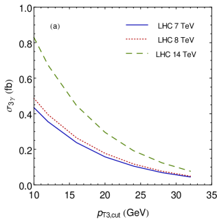
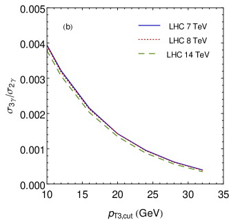
Figure 3: (a), Cross sections of the SM tri-photon production at the LHC; (b), ratios of the cross sections of the SM tri-photon production to the ones of diphoton production. The selection cuts are applied to both the tri-photon and diphoton events.

By the same assumptions as in Section IV.2, the expected background event rate is about $1.1\times 10^{5}$ for the diphoton channel at the LHC of 14 TeV and $\mathcal{L}=100\,fb^{-1}$. Simply multiplying it with the ratio $\sigma_{3\gamma}/\sigma_{2\gamma}$, we estimate a background rate of about 242 for the tri-photon final state. Similarly, using the numbers in Tables. 7-9, the expected signal event rates are about $0.8$, $16$ and $24$ for the SM, models B and C respectively. We can see that the signal rates of the models B and C are of the similar size as the $1\sigma$ statistical fluctuation of the background. Thus although the associated production mode shows a large distinction between the SM and the alternative models, i.e., models B and C, but it requires a high luminosity for the experimental measurements, e.g., around 900 (400) $fb^{-1}$ in order to discriminate the SM with the model B (C) at $3\sigma$ C.L. Also note that for a variation of the model B where the charm quark coupling is dominant instead of the bottom quark, the associated production rate can be further enhanced by about a factor of 4 from the electric charge.

V Conclusions

We performed a study on differentiating the direct production mechanisms of the newly discovered Higgs-like boson at the LHC based on several inclusive observables introduced, including the ratios of the production rates at different colliders and energies, the centrality ratios of the resonance, and the ratios of the rates of associated production with a photon to the ones of direct production. Above ratios reveal neither the parton constituents nor initial state radiations involved in the production mechanisms, and are independent of the couplings to the decay products. We select three benchmark models, including the SM Higgs boson, to illustrate how the theoretical predictions of the above ratios are different for the $gg$, $b\bar{b}(c\bar{c})$, and $q\bar{q}$ (flavor universal) initial states in the direct production. The theoretical uncertainties of the predictions are also discussed. All three models are found to be in good agreement with inclusive rate ratios from current measurements at the Tevatron and LHC. Moreover, we show expectations from further LHC measurements with high luminosities. The centrality ratio measurements are supposed to be able to separate the $gg$ or $b\bar{b}(c\bar{c})$ initial states with $q\bar{q}$. The tri-photon signal from the associated production may even differentiate the $gg$ initial states with $b\bar{b}(c\bar{c})$ or $q\bar{q}$ in the direct production.

- (1) G. Aad et al. [ATLAS Collaboration], Phys. Lett. B 716 (2012) 1 [arXiv:1207.7214 [hep-ex]].
- (2) S. Chatrchyan et al. [CMS Collaboration], Phys. Lett. B 716 (2012) 30 [arXiv:1207.7235 [hep-ex]].
- (3) L. D. Landau, Dokl. Akad. Nauk Ser. Fiz. 60 (1948) 207.
- (4) C. -N. Yang, Phys. Rev. 77, 242 (1950).
- (5) S. Y. Choi, D. J. Miller, 2, M. M. Muhlleitner and P. M. Zerwas, Phys. Lett. B 553 (2003) 61 [hep-ph/0210077].
- (6) Y. Gao, A. V. Gritsan, Z. Guo, K. Melnikov, M. Schulze and N. V. Tran, Phys. Rev. D 81 (2010) 075022 [arXiv:1001.3396 [hep-ph]].
- (7) A. De Rujula, J. Lykken, M. Pierini, C. Rogan and M. Spiropulu, Phys. Rev. D 82 (2010) 013003 [arXiv:1001.5300 [hep-ph]].
- (8) C. Englert, C. Hackstein and M. Spannowsky, Phys. Rev. D 82 (2010) 114024 [arXiv:1010.0676 [hep-ph]].
- (9) J. Ellis and D. S. Hwang, JHEP 1209 (2012) 071 [arXiv:1202.6660 [hep-ph]].
- (10) S. Bolognesi, Y. Gao, A. V. Gritsan, K. Melnikov, M. Schulze, N. V. Tran and A. Whitbeck, Phys. Rev. D 86 (2012) 095031 [arXiv:1208.4018 [hep-ph]].
- (11) S. Y. Choi, M. M. Muhlleitner and P. M. Zerwas, Phys. Lett. B 718 (2013) 1031 [arXiv:1209.5268 [hep-ph]].
- (12) J. Ellis, R. Fok, D. S. Hwang, V. Sanz and T. You, Eur. Phys. J. C 73 (2013) 2488 [arXiv:1210.5229 [hep-ph]].
- (13) C. Englert, D. Goncalves-Netto, K. Mawatari and T. Plehn, JHEP 1301 (2013) 148 [arXiv:1212.0843 [hep-ph]].
- (14) S. Banerjee, J. Kalinowski, W. Kotlarski, T. Przedzinski and Z. Was, Eur. Phys. J. C 73 (2013) 2313 [arXiv:1212.2873 [hep-ph]].
- (15) T. Modak, D. Sahoo, R. Sinha and H. -Y. Cheng, arXiv:1301.5404 [hep-ph].
- (16) D. Boer, W. J. d. Dunnen, C. Pisano and M. Schlegel, Phys. Rev. Lett. 111 (2013) 032002 [arXiv:1304.2654 [hep-ph]].
- (17) J. Frank, M. Rauch and D. Zeppenfeld, arXiv:1305.1883 [hep-ph].
- (18) C. Englert, D. Goncalves, G. Nail and M. Spannowsky, Phys. Rev. D 88 (2013) 013016 [arXiv:1304.0033 [hep-ph]].
- (19) R. Boughezal, T. J. LeCompte and F. Petriello, arXiv:1208.4311 [hep-ph].
- (20) J. Ellis, D. S. Hwang, V. Sanz and T. You, JHEP 1211 (2012) 134 [arXiv:1208.6002 [hep-ph]].
- (21) A. Alves, Phys. Rev. D 86 (2012) 113010 [arXiv:1209.1037 [hep-ph]].
- (22) C. -Q. Geng, D. Huang, Y. Tang and Y. -L. Wu, Phys. Lett. B 719 (2013) 164 [arXiv:1210.5103 [hep-ph]].
- (23) A. Djouadi, R. M. Godbole, B. Mellado and K. Mohan, Phys. Lett. B 723 (2013) 307 [arXiv:1301.4965 [hep-ph]].
- (24) [ATLAS Collaboration], ATLAS-CONF-2013-029.
- (25) [ATLAS Collaboration], ATLAS-CONF-2013-040.
- (26) G. Aad et al. [ATLAS Collaboration], Phys. Lett. B 726, 120 (2013) [arXiv:1307.1432 [hep-ex]].
- (27) [CMS Collaboration], CMS-PAS-HIG-13-002.
- (28) T. Plehn, D. L. Rainwater and D. Zeppenfeld, Phys. Rev. Lett. 88 (2002) 051801 [hep-ph/0105325].
- (29) P. P. Giardino, K. Kannike, M. Raidal and A. Strumia, JHEP 1206 (2012) 117 [arXiv:1203.4254 [hep-ph]].
- (30) M. Rauch, arXiv:1203.6826 [hep-ph].
- (31) A. Azatov, R. Contino, D. Del Re, J. Galloway, M. Grassi and S. Rahatlou, JHEP 1206 (2012) 134 [arXiv:1204.4817 [hep-ph]].
- (32) I. Low, J. Lykken and G. Shaughnessy, Phys. Rev. D 86 (2012) 093012 [arXiv:1207.1093 [hep-ph]].
- (33) D. Carmi, A. Falkowski, E. Kuflik, T. Volansky and J. Zupan, JHEP 1210 (2012) 196 [arXiv:1207.1718 [hep-ph]].
- (34) T. Plehn and M. Rauch, Europhys. Lett. 100 (2012) 11002 [arXiv:1207.6108 [hep-ph]].
- (35) A. Djouadi, Eur. Phys. J. C 73 (2013) 2498 [arXiv:1208.3436 [hep-ph]].
- (36) A. Djouadi, Phys. Rept. 459 (2008) 1 [hep-ph/0503173].
- (37) Y. Meng, Z. ’e. Surujon, A. Rajaraman and T. M. P. Tait, JHEP 1302 (2013) 138 [arXiv:1210.3373 [hep-ph]].
- (38) N. Arkani-Hamed, S. Dimopoulos and G. R. Dvali, Phys. Lett. B 429 (1998) 263 [hep-ph/9803315].
- (39) L. Randall and R. Sundrum, Phys. Rev. Lett. 83 (1999) 3370 [hep-ph/9905221].
- (40) M. L. Mangano and J. Rojo, JHEP 1208, 010 (2012) [arXiv:1206.3557 [hep-ph]].
- (41) M. Fierz, Helv. Phys. Acta 12, 3 (1939).
- (42) H. van Dam and M. J. G. Veltman, Nucl. Phys. B 22, 397 (1970).
- (43) K. Hagiwara, J. Kanzaki, Q. Li and K. Mawatari, Eur. Phys. J. C 56, 435 (2008) [arXiv:0805.2554 [hep-ph]].
- (44) J. Beringer et al. [Particle Data Group Collaboration], Phys. Rev. D 86 (2012) 010001.
- (45) K. G. Chetyrkin, J. H. Kuhn and M. Steinhauser, Comput. Phys. Commun. 133 (2000) 43 [hep-ph/0004189].
- (46) S. Dittmaier, S. Dittmaier, C. Mariotti, G. Passarino, R. Tanaka, S. Alekhin, J. Alwall and E. A. Bagnaschi et al., arXiv:1201.3084 [hep-ph].
- (47) M. Wiesemann, Nucl. Phys. Proc. Suppl. 234 (2013) 25 [arXiv:1211.0977 [hep-ph]].
- (48) C. Anastasiou, S. Buehler, F. Herzog and A. Lazopoulos, JHEP 1112 (2011) 058 [arXiv:1107.0683 [hep-ph]].
- (49) J. Gao, M. Guzzi, J. Huston, H. -L. Lai, Z. Li, P. Nadolsky, J. Pumplin and D. Stump et al., arXiv:1302.6246 [hep-ph].
- (50) A. D. Martin, W. J. Stirling, R. S. Thorne and G. Watt, Eur. Phys. J. C 63 (2009) 189 [arXiv:0901.0002 [hep-ph]].
- (51) R. D. Ball, V. Bertone, S. Carrazza, C. S. Deans, L. Del Debbio, S. Forte, A. Guffanti and N. P. Hartland et al., Nucl. Phys. B 867 (2013) 244 [arXiv:1207.1303 [hep-ph]].
- (52) R. D. Ball, S. Carrazza, L. Del Debbio, S. Forte, J. Gao, N. Hartland, J. Huston and P. Nadolsky et al., JHEP 1304 (2013) 125 [arXiv:1211.5142 [hep-ph]].
- (53) S. Catani and M. Grazzini, Phys. Rev. Lett. 98 (2007) 222002 [hep-ph/0703012].
- (54) A. Abbasabadi, D. Bowser-Chao, D. A. Dicus and W. W. Repko, Phys. Rev. D 58 (1998) 057301 [hep-ph/9706335].
- (55) The ATLAS collaboration, ATLAS-CONF-2013-072.
- (56) C. J. Glosser and C. R. Schmidt, JHEP 0212, 016 (2002) [hep-ph/0209248].
- (57) G. Bozzi, S. Catani, D. de Florian and M. Grazzini, Phys. Lett. B 564, 65 (2003) [hep-ph/0302104].
- (58) B. Field, Phys. Rev. D 70, 054008 (2004) [hep-ph/0405219].
- (59) B. Field, hep-ph/0407254.
- (60) A. Belyaev, P. M. Nadolsky and C. -P. Yuan, JHEP 0604, 004 (2006) [hep-ph/0509100].
- (61) T. Aaltonen et al. [CDF and D0 Collaborations], Phys. Rev. D 88, 052014 (2013) [arXiv:1303.6346 [hep-ex]].
- (62) The ATLAS collaboration, ATLAS-CONF-2013-108.
- (63) [CMS Collaboration], CMS-PAS-HIG-13-004.
- (64) J. Alwall, P. Demin, S. de Visscher, R. Frederix, M. Herquet, F. Maltoni, T. Plehn and D. L. Rainwater et al., JHEP 0709 (2007) 028 [arXiv:0706.2334 [hep-ph]].