Distributed computation of equilibria in misspecified convex stochastic Nash games

Abstract

The distributed computation of Nash equilibria is assuming growing relevance in engineering where such problems emerge in the context of distributed control. Accordingly, we present schemes for computing equilibria of two classes of static stochastic convex games complicated by a parametric misspecification, a natural concern in the control of large-scale networked engineered system. In both schemes, players learn the equilibrium strategy while resolving the misspecification: (1) Monotone stochastic Nash games: We present a set of coupled stochastic approximation schemes distributed across agents in which the first scheme updates each agent’s strategy via a projected (stochastic) gradient step while the second scheme updates every agent’s belief regarding its misspecified parameter using an independently specified learning problem. We proceed to show that the produced sequences converge in an almost-sure sense to the true equilibrium strategy and the true parameter , respectively. Surprisingly, convergence in the equilibrium strategy achieves the optimal rate of convergence in a mean-squared sense with a quantifiable degradation in the rate constant; (2) Stochastic Nash-Cournot games with unobservable aggregate output: We refine (1) to a Cournot setting where we assume that the tuple of strategies is unobservable while payoff functions and strategy sets are public knowledge through a common knowledge assumption. By utilizing observations of noise-corrupted prices, iterative fixed-point schemes are developed, allowing for simultaneously learning the equilibrium strategies and the misspecified parameter in an almost-sure sense.

I Introduction

In networked engineered systems, a common challenge lies in designing distributed control architectures that ensure the satisfaction of a system-wide criterion in environments complicated by nonlinearity, uncertainty, and dynamics. Such control-theoretic problems take on a variety of forms and arise in a variety of networked settings, including networks of unmanned aerial vehicles (UAVs), traffic networks, wireline and wireless communication networks, and energy systems, amongst others. These systems are often characterized by the absence of a designated central entity that either has system-wide control or has access to global information. Consequently, control is effected through distributed decision-making and local interactions that rely on limited information. Game-theoretic approaches represent an avenue for designing such protocols. Game theory has seen wide applicability in the social, economic, and engineered sciences in a largely descriptive role. There has been immense recent interest in a prescriptive role [2] that considers designing a game whose equilibria represent the solutions to the control problem of interest [3, 4]; consequently, the distributed learning of Nash equilibria assumes immediate relevance in the management of networked systems. Learning in Nash games has seen much study in the last several decades [5, 6, 7, 8]. In continuous strategy regimes, convex static games find significance in engineered systems such as communication networks  [9, 10, 11, 12] and signal processing [13, 14].

An oft-used assumption in game-theoretic models requires that player payoffs are public knowledge, allowing every player to correctly forecast the choices of his adversaries. As noted by Kirman [15], a firm’s view of the game may be corrupted or misspecified in at least two distinct ways in a Cournot setting where firms decide production levels given a price function: (i) a firm might have a correct description of the price function but an incorrect estimate of its parameters; and (ii) it may have an incorrect structure of the price function and incorrectly conclude that prediction errors are a consequence of misspecified parameters. Kirman [15] considered such a learning process, and showed that by observing true demand, the suggested learning process guarantees that the firm strategies converge to the noncooperative Nash equilibrium. Further inspiration may be drawn from studies by Bischi [16, 17], Szidarovsky [18, 19], amongst others [20], where firms competing in a deterministic Nash-Cournot game learn a parameter of the demand function while playing the game repeatedly. Note that an inherent assumption of a low discount rate is imposed that discounts the future effect of any player’s strategies. Analogous questions of optimization and estimation have also been studied by Cooper et al. [21] who consider a joint process of forecasting and optimization in a regime where the underlying model may be erroneous, demonstrating that the resulting revenues can systematically reduce over time.

When designing protocols for practical engineered systems, particularly in the absence of a centralized controller, the associated parameters of the utility functions may often be misspecified. For instance, in power market models that enlist Nash-Cournot models [22, 23], the precise nature of the price function is assumed to be given. Similarly, the expected capacity or availability of renewable generation assets is rarely known a priori. Similarly, when developing distributed protocols for networked UAVs, the prescribed utility functions may rely on agent-specific information that can only be learnt through observations. Faced by such challenges, our goal lies in the development and analysis of general purpose algorithms that combine computation of Nash equilibria with a learning phase to correct misspecification.

Motivation: This research is motivated by the absence of general-purpose distributed schemes with asymptotic convergence and rate guarantees for learning equilibria in the face of imperfect information. Such problems emerge from stochastic generalizations of problems arising in communication networks [10, 24, 11, 12], signal processing [13, 14], and power markets [22]. Accordingly, we present two distributed learning schemes in which agents learn their Nash strategy while correcting the misspecification in their payoffs:
(1) Stochastic gradient schemes for stochastic Nash games: In Section II, we present a distributed stochastic approximation framework in which every agent makes two projected gradient updates: Every agent first updates its belief regarding the equilibrium strategy by using the sampled gradient of its payoff function and subsequently updates its belief regarding the misspecified parameter through a similar gradient update. The resulting sequence of equilibrium and parameter estimates are shown to converge to their true counterparts in an almost sure sense. Notably, we show that the mean-squared error of the equilibrium estimates converges to zero at the optimal rate ${\cal O}(1/K)$ despite the presence of misspecification where $K$ denotes the number of gradient steps.
(2) Iterative fixed-point schemes for stochastic Nash-Cournot games: In Section III, we consider a Cournot regime where aggregate output is unobservable and one parameter of the demand function is misspecified. Under common-knowledge, agents develop an estimate of aggregate output and the misspecified price function parameter by observing noisy prices. These estimates allow developing an iterative fixed-point scheme that produces iterates that are shown to converge to the Nash-Cournot equilibrium in an almost-sure sense. Additionally, firms learn the true parameter in an almost-sure sense. The result can be extended to nonlinear price functions.

Remark: We make two remarks before proceeding. (a) First, in (1), the learning problem is constructed independently of the computational problem through a set of observations while in (2), the learning is affected by the computational step (akin to multi-armed bandit problems). (b) Second, we comment on the sequential two-stage framework for resolving misspecification:

Step 1. Learn $$\theta^{*} x^{*}(\theta^{*})$$       Step 2. Compute ,

where $\theta^{*}$ is to be learnt and $x^{*}(\theta^{*})$ is the (stochastic) Nash equilibrium, given $\theta^{*}$. Unfortunately, a sequential approach is complicated by several challenges. First, Step 1. needs to be completed in a finite number of iterations, practically impossible for stochastic learning problems. Second, premature termination of Step 1. leads to an erroneous estimate $\hat{\theta}$ resulting in an incorrect Nash equilibrium $\hat{x}$. In fact, in stochastic regimes, such avenues do not lead to asymptotic convergence and at best provide approximate solutions. We observe from preliminary numerics reveal that sequential schemes may perform orders of magnitude worse when compared with iterative fixed-point schemes (see Table IV(b)).

The rest of the paper is organized as follows. In Section II, we define and resolve a misspecified stochastic Nash game and present a joint set of stochastic approximation schemes that collectively allow for learning equilibria and resolving misspecification. In Section III, we develop iterative fixed-point schemes in Cournot settings where aggregate output is unobservable. Empirical studies and conclusions are provided in Sections IV and V, respectively. Throughout the paper, $\|x\|$ denotes the Euclidean norm of a vector $x$, i.e., $\|x\|=\sqrt{x^{T}x}$ while $\Pi_{K}(u)$ denotes the Euclidean projection of $u$ onto a set $K$, i.e., $\Pi_{K}(x)\triangleq\mathop{\rm argmin}_{y\in K}\|x-y\|$. A square matrix $H$ is said to be a $\mathbf{P}$-matrix if every principal minor of $H$ is positive. Similarly, $H$ is a $\mathbf{P_{0}}$-matrix if every principal minor of $H$ is nonnegative.

II Gradient-based schemes for convex games

II-A Problem description, assumptions and background

We consider an $N-$person stochastic Nash game in which the $i$th player solves Opt$(x_{-i})$:

$$\begin{aligned} \min_{x_{i}\in K_{i}}&\quad{\color[rgb]{0,0,0}{f_{i}(x;\theta^{*})}}\triangleq\mathbb{E}\!\left[f_{i}(x;\theta^{*},{\color[rgb]{0,0,0}{\xi}})\right]\end{aligned} (x_{-i})$$ (Opt)

where $K_{i}\subseteq\mathbb{R}^{n_{i}}$, $\theta^{*}\in\mathbb{R}^{m}$, $\xi:\Omega\to\mathbb{R}^{d}$ defined on a probability space $({\color[rgb]{0,0,0}{\Omega}},{\mathcal{F}}_{x},\mathbb{P}_{x})$, $n=\sum_{i=1}^{N}n_{i}$, and $f_{i}:\mathbb{R}^{n}\times\mathbb{R}^{m}\times\mathbb{R}^{d}\to\mathbb{R}$ is a real-valued function in $x_{i}$, $x_{-i}\triangleq(x_{j})_{i\neq j=1}^{N}$, $\theta$ and ${\color[rgb]{0,0,0}{\xi}}$. The associated Nash equilibrium is given by a tuple $x^{*}=(x_{i}^{*})_{i=1}^{N}$ where $x_{i}^{*}\in\textrm{SOL}(\textrm{Opt}(x_{-i}^{*}))$ for $i=1,\ldots,N,$ $\textrm{SOL}(\textrm{Opt}(x_{-i}^{*}))$ denotes the solution of $\textrm{Opt}(x_{-i})$ and under suitable convexity and differentiability requirements (see (A1) below), by invoking [25, Th. 7.46], $x^{*}$ is a solution to a stochastic variational inequality problem VI$(K,F(\cdot;\theta^{*}))$ where

$$\begin{aligned} K\triangleq\prod_{i=1}^{N}K_{i}\mbox{ and }F(x;\theta)\triangleq{\color[rgb]{0,0,0}{\begin{pmatrix}F_{i}(x;\theta)\end{pmatrix}_{i=1}^{N}\triangleq}}\begin{pmatrix}\mathbb{E}\!\left[\nabla_{x_{i}}f_{i}(x;\theta,{\color[rgb]{0,0,0}{\xi}})\right]\end{pmatrix}_{i=1}^{N},\end{aligned}$$ (1)

respectively. It may be recalled that VI$(K,F)$ requires an $x\in K$ satisfying

$$(y-x)^{T}F(x;\theta^{*})\geq 0,\quad\,\textrm{for all }y\in K.$$ (2)

Our overall goal lies in computing equilibria when $\theta^{*}$ is unavailable or misspecified but can be learnt by a possibly stochastic learning problem.

Learning scheme

In this section, we consider the estimation of $\theta^{*}$ through the solution of a suitably defined stochastic convex learning problem [26]:

$$\min_{\theta\in\Theta}\quad g(\theta)\triangleq\mathbb{E}[g(\theta;\eta)],$$ (3)

where $\Theta\subseteq\mathbb{R}^{m}$ is a closed and convex set, $\eta:{\color[rgb]{0,0,0}{\Lambda}}\to\mathbb{R}^{p}$ is a random variable defined on a probability space $(\Lambda,\mathcal{F}_{\theta},\mathbb{P}_{\theta})$, and $g:\Theta\times{\color[rgb]{0,0,0}{\mathbb{R}^{p}}}\to\mathbb{R}$ is a real-valued learning metric function (such as a regression metric constructed from a set of observations). Consequently, $\theta^{*}$ may be learnt through a stochastic gradient scheme of the form for $k\geq 0$:

$$\theta_{i}^{k+1}:=\Pi_{\Theta}\left(\theta_{i}^{k}-\alpha_{i}^{k}\nabla_{\theta}g(\theta_{i}^{k};{\color[rgb]{0,0,0}{\eta_{i}^{k}}})\right),\,i=1,\ldots,N.$$ (4)

We emphasize that this learning problem is unrelated to the computational process and is a built from a set of independently collected observations.

Distributed computational scheme

We consider a distributed stochastic approximation scheme where the $i$th agent employs its belief regarding $\theta^{*}$ to take a (stochastic) gradient step for $i=1,\ldots,N$:

$$x_{i}^{k+1}:=\Pi_{K_{i}}\left(x_{i}^{k}-\gamma_{i}^{k}\nabla_{x_{i}}f_{i}(x^{k};{\color[rgb]{0,0,0}{\theta_{i}^{k},\xi_{i}^{k}}})\right),\quad k\geq 0,$$ (5)

where $\gamma_{i}^{k}$ and $\nabla_{x_{i}}f_{i}(x^{k};{\color[rgb]{0,0,0}{\theta_{i}^{k},\xi_{i}^{k}}})$ denotes the steplength and sampled gradient used by player $i$ at step $k$. While a fully rational agent would always take a best response step, in stochastic settings, the complexity of this step might be significant. In bounded rational regimes where computational constraints are imposed, an alternative lies in computing other steps such as the gradient-response (cf. [27, 28]). An alternative motivation arises from distributed control/optimization settings where a “game” is designed whose equilibrium is a desirable solution to a suitably defined control problem. Here, a distributed protocol for computing an equilibrium can be designed and gradient-based approaches can be adopted (cf. [2, 3, 4]). We propose a game-theoretic extension of that developed in [29, 30]. We may specify our joint simulation-based scheme for learning and computation as follows:

Algorithm I: Gradient response and learning. Let ${\theta_{i}^{0}}\,\in\,\Theta$, ${\color[rgb]{0,0,0}{x^{0}}}\,\in\,K$, $\{\gamma_{i}^{k},\alpha_{i}^{k}\}\,>\,0$ , for $i=1,\ldots,N$, and $k\,=\,0$. Step 1: $\displaystyle\left.\begin{aligned} \mathbf{(Comp)}\,x_{i}^{k+1}&:=\Pi_{K_{i}}\left(x_{i}^{k}-\gamma_{i}^{k}\nabla_{x_{i}}f_{i}(x^{k};{\theta_{i}^{k}},\xi_{i}^{k})\right),\\ \mathbf{(Learn)}\,\,\theta_{i}^{k+1}&:={\Pi_{\Theta}\left(\theta_{i}^{k}-\alpha_{i}^{k}\nabla_{\theta}g(\theta_{i}^{k};\eta_{i}^{k})\right)},\end{aligned}\right\}i=1,\ldots,N;$ (6) Step 2: if $k>\bar{K}$, stop; else $k:=k+1$ and go to Step 1.

We now present the main assumptions employed in deriving convergence properties of Algorithm I. (A1) enforces convexity assumptions that allow for deriving sufficient equilibrium conditions given by VI$(X,F)$ while the monotonicity requirements on $F$ allow for claiming the existence of a unique equilibrium. Lipschitzian requirements of $F$ aid in deriving subsequent convergence and rate statements. Furthermore, a breadth of learning problems (such as regression, classification etc. [26]) are convex. The requirements imposed by (A2) are standard in developing distributed protocols while (A3) imposes assumptions on the conditional first and second moments common in stochastic approximation literature [31, 32, 33].

Assumption 1 (A1)

For $i=1,\ldots,N$, suppose the function $f_{i}(x;\theta)$ is convex and continuously differentiable function in $x_{i}$ for every $x_{-i}\in\prod_{j\neq i}K_{j}$ and every $\theta\in\Theta$. Furthermore, suppose $\Theta$ is a closed, convex, and bounded set and for $i=1,\ldots,N$, $K_{i}\subseteq\mathbb{R}^{n_{i}}$ is a nonempty, closed, convex and bounded set. Furthermore, suppose the following hold:(a) For every $\theta\in\Theta$, $F(x;\theta)$ is both strongly monotone and Lipschitz continuous in $x$ with constants $\mu_{x}$ and $L_{x}$; for every $\theta$, $(F(x;\theta)-F(y;\theta))^{T}(x-y)\geq\mu_{x}\|x-y\|^{2}$ and $\|F(x;\theta)-F(y;\theta)\|\leq L_{x}\|x-y\|$; (b) For every $x\in K$, $F(x;\theta)$ is Lipschitz continuous in $\theta$ with constant $L_{\theta}$; (c) The function $g(\theta)$ is strongly convex and continuously differentiable with Lipschitz continuous gradients in $\theta$ with convexity constant $\mu_{\theta}$ and Lipschitz constant $C_{\theta}$, respectively; $(\nabla g(\theta_{1})-\nabla g(\theta_{2}))^{T}(\theta_{1}-\theta_{2})\geq\mu_{\theta}\|\theta_{1}-\theta_{2}\|^{2}$, and $\|\nabla g(\theta_{1})-\nabla g(\theta_{2})\|\leq C_{\theta}\|\theta_{1}-\theta_{2}\|$.

Note that monotone Nash games include stable Nash games, a class of games for which a range of evolutionary dynamics allow for convergence to Nash equilibria [34, 35].

Assumption 2 (A2)

For $i=1,\ldots,N$, the $i$th agent knows only his objective $f_{i}$ and strategy set $K_{i}$ and the parameter set $\Theta$. Furthermore, the vector $x$ is assumed to be observable.

We define a new probability space $(Z,\mathcal{F},\mathbb{P})$, where $Z\triangleq\Omega\times\Lambda$, $\mathcal{F}\triangleq\mathcal{F}_{x}\times\mathcal{F}_{\theta}$ and $\mathbb{P}\triangleq\mathbb{P}_{x}\times\mathbb{P}_{\theta}$. For $i=1,\ldots,N$, suppose $w_{i}^{k}\triangleq\nabla_{x_{i}}f_{i}(x^{k};\theta^{k}_{i},{\color[rgb]{0,0,0}{\xi_{i}^{k}}})-\nabla_{x_{i}}f_{i}(x^{k};\theta^{k}_{i})$ and $v^{k}_{i}\triangleq\nabla_{\theta}g(\theta^{k}_{i};{\color[rgb]{0,0,0}{\eta_{i}^{k}}})-\nabla_{\theta}g(\theta^{k}_{i})$. $\mathcal{F}_{k}$ denotes the sigma-field generated by $(x^{0},\theta^{0})$ and errors $(w^{l},v^{l})$ for $l=0,1,\cdots,k-1$, i.e., $\mathcal{F}_{0}={\color[rgb]{0,0,0}{\sigma}}\left\{(x^{0},\theta^{0})\right\}$ and $\mathcal{F}_{k}={\color[rgb]{0,0,0}{\sigma}}\left\{(x^{0},\theta^{0}),\left((w^{l},v^{l}),l=0,1,\cdots,k-1\right)\right\}$ for $k\geq 1.$

Assumption 3 (A3)

(a) Unbiasedness: $\mathbb{E}[{\color[rgb]{0,0,0}{w_{i}^{k}}}\mid\mathcal{F}_{k}]=0$ and $\mathbb{E}[v_{i}^{k}\mid\mathcal{F}_{k}]=0$ $a.s.$ for all $k$ and $i$; (b) Bounded second moments: $\mathbb{E}[\|{\color[rgb]{0,0,0}{w_{i}^{k}}}\|^{2}\mid\mathcal{F}_{k}]\leq\nu^{2}_{x}$ and $\mathbb{E}[\|v_{i}^{k}\|^{2}\mid\mathcal{F}_{k}]\leq\nu^{2}_{\theta}$ $a.s.$ for all $k,i$.

To construct distributed schemes requiring no coordination in terms of setting parameters, we allow each agent to independently set steplengths and as long as a suitable relationship between these steplengths holds, convergence follows. Specifically, the $i$th agent employs a diminishing steplength sequence given by $\gamma_{i}^{k}.$ Furthermore, we define $\gamma_{\min}^{k}\triangleq\min_{1\leq i\leq N}\{\gamma_{i}^{k}\}$ and $\gamma_{\max}^{k}\triangleq\max_{1\leq i\leq N}\{\gamma_{i}^{k}\}$ for all $k$. Similarly, we define $\alpha_{\min}^{k}\triangleq\min_{1\leq i\leq N}\{\alpha_{i}^{k}\}$ and $\alpha_{\max}^{k}\triangleq\max_{1\leq i\leq N}\{\alpha_{i}^{k}\}$ for all $k$. Then, we can make the following assumptions on the steplengths of the algorithm.

Assumption 4 (Steplength requirements, A4)

Let $\{\gamma_{i}^{k}\}$ and $\{\alpha_{i}^{k}\}$ be chosen such that: (a) $\sum_{k=1}^{\infty}\gamma_{\min}^{k}=\infty$, $\sum_{k=1}^{\infty}(\gamma_{\max}^{k})^{2}<\infty$, $\sum_{k=1}^{\infty}(\alpha_{\max}^{k})^{2}<\infty$; (b) $\lim_{k\to\infty}\frac{\gamma_{\max}^{k}-\gamma_{\min}^{k}}{\gamma_{\max}^{k}}=0$; (c) $\alpha_{\min}^{k}\geq\gamma_{\max}^{k}L_{\theta}^{2}/(\mu_{x}\mu_{\theta})$ for sufficiently large $k$, $\lim_{k\to\infty}\frac{(\alpha_{\max}^{k})^{2}}{\gamma_{\max}^{k}}=0.$

Notice that (a)$\sum_{k=1}^{\infty}\gamma_{\min}^{k}=\infty$ and (c) $\alpha_{\min}^{k}\geq\gamma_{\max}^{k}L_{\theta}^{2}/(\mu_{x}\mu_{\theta})$ for sufficiently large $k$ implies that $\sum_{k=1}^{\infty}\alpha_{\min}^{k}=\infty$. A natural concern is whether the rule that relates the steplengths can be implemented in a distributed fashion without coordination. We propose a rule, first suggested by  [36], in which every agent chooses a positive integer and the required coordination statement holds. We view this as a protocol that may be employed for developing distributed schemes. The next result ensures that for such a choice, the required assumptions hold [36].

Lemma 1 (Choice of steplength sequences)

Let $\{\gamma_{i}^{k}\}$ and $\{\alpha_{i}^{k}\}$ be chosen such that $\gamma_{i}^{k}=\frac{1}{(k+N_{i})^{\alpha}}$ and $\alpha_{i}^{k}=\frac{1}{(k+M_{i})^{\beta}}$ where $N_{i}$ and $M_{i}$ are positive integers and $\frac{1}{2}<\beta<\alpha<1$. Then, (A4) holds.

We state three results (without proof) that will be employed in developing our convergence statements, of which the first two are relatively well-known super-martingale convergence results (cf. [37, Lemma 10,  Pg. 49–50])

Lemma 2

Let ${\color[rgb]{0,0,0}{s^{k}}}$ be a sequence of nonnegative random variables adapted to $\sigma$-algebra $\mathcal{F}_{k}$ and such that $\mathbb{E}[{\color[rgb]{0,0,0}{s^{k+1}}}\mid\mathcal{F}_{k}]\leq(1-{\color[rgb]{0,0,0}{u^{k}}}){\color[rgb]{0,0,0}{s^{k}}}+{\color[rgb]{0,0,0}{\beta^{k}}}$ for all $k\geq 0$ almost surely, where $0\leq{\color[rgb]{0,0,0}{u^{k}}}\leq 1$, ${\color[rgb]{0,0,0}{\beta^{k}}}\geq 0$, and $\sum_{k=0}^{\infty}{\color[rgb]{0,0,0}{u^{k}}}=\infty$, $\sum_{k=0}^{\infty}\beta^{k}<\infty$ and $\lim_{k\to\infty}\frac{\beta^{k}}{u^{k}}=0$. Then, ${\color[rgb]{0,0,0}{s^{k}}}\to 0$ in an a.s. sense.

Lemma 3

Let $s^{k}$, $u^{k}$, $\beta^{k}$ and $\gamma^{k}$ be non-negative random variables adapted to $\sigma$-algebra $\mathcal{F}_{k}$. If $\mathbb{E}[s^{k+1}\mid\mathcal{F}_{k}]\leq(1+u^{k})s^{k}-\gamma^{k}+\beta^{k}$ for all $k\geq 0$ a.s. where $\sum_{k=0}^{\infty}u^{k}<\infty$ and $\sum_{k=0}^{\infty}\beta^{k}<\infty$ both hold a.s., then $\{s^{k}\}$ is convergent in an a.s. sense and $\sum_{k=0}^{\infty}\gamma_{k}<\infty$ a.s.

Finally, we present a contraction result reliant on monotonicity and Lipschitzian requirements.

Lemma 4

(cf. [38, Theorem 12.1.2, Pg. 1109]) Let $H:K\to\mathbb{R}^{n}$ be a strongly monotone map over $K$ with constant $\mu$, and Lipschitz continuous over $K$ with constant $L$. If $q\triangleq\sqrt{1-2\mu\gamma+\gamma^{2}L^{2}}$, then for any $\gamma>0$, we have the following: $\|\Pi_{K}(x-\gamma H(x))-\Pi_{K}(y-\gamma H(y))\|{\color[rgb]{0,0,0}{\leq\|x-y-\gamma(H(x)-H(y))\|}}\leq q\|x-y\|.$

II-B Convergence Analysis

We begin with a contraction statement for the sequence of iterates produced by Algorithm I.

Lemma 5

Suppose (A1), (A2), (A3) and (A4) hold. Let $\{x^{k},\theta^{k}\}$ be computed via Algorithm I. For any $k\geq 0$, $\mathbb{E}\left[\|x^{k+1}-x^{*}\|^{2}\mid\mathcal{F}_{k}\right]\leq\zeta_{k}\|x^{k}-x^{*}\|^{2}+\beta_{k}$, where $\zeta_{k}=1-\gamma_{\max}^{k}\mu_{x}+2(\gamma_{\max}^{k}-\gamma_{\min}^{k})L_{x}+2(\gamma_{\max}^{k})^{2}L_{x}^{2}$ and $\beta_{k}=(2(\gamma_{\max}^{k})^{2}L_{\theta}^{2}+\gamma_{\max}^{k}L_{\theta}^{2}/\mu_{x})\sum_{i=1}^{N}\|\theta_{i}^{k}-\theta^{*}\|^{2}+{\color[rgb]{0,0,0}{N}}(\gamma_{\max}^{k})^{2}\nu_{x}^{2}$.

We may now prove our main a.s. convergence result for the sequences $\{x^{k}\}$ and $\{\theta^{k}\}$.

Theorem 1

Suppose (A1), (A2), (A3) and (A4) hold. Let $\{x^{k},\theta^{k}\}$ be computed via Algorithm I. Then, $x^{k}\buildrel a.s.\over{\longrightarrow}x^{*}$ and $\theta_{i}^{k}\buildrel a.s.\over{\longrightarrow}\theta^{*}$ as $k\rightarrow\infty$ for all $i$.

Finally, we conclude this section with a non-asymptotic error bound that demonstrates that the joint scheme displays the optimal rate of ${\cal O}(1/K)$ in mean-squared error.

Theorem 2

Suppose (A1), (A2) and (A3) hold. Suppose $\gamma_{i}^{k}=\lambda_{x,i}/k$ and $\alpha_{i}^{k}=\lambda_{\theta,i}/k$. Let $\mathbb{E}[\|F_{i}(x^{k};{\theta_{i}^{k}})+w_{i}^{k}\|^{2}]\leq{\color[rgb]{0,0,0}{M_{x}}}^{2}/N$ and $\mathbb{E}[\|\nabla_{\theta}g(\theta_{i}^{k})+v_{i}^{k}\|^{2}]\leq M_{\theta}^{2}$ for all $x^{k}\in K$ and $\theta_{i}^{k}\in\Theta$. Let $\{x^{k},\theta^{k}\}$ be computed via Algorithm I. Then, there exist constants $Q_{\theta}$ and $Q_{x,\theta}$ such that the following hold after $K$ iterations: $\mathbb{E}[\|\theta_{i}^{K}-\theta^{*}\|^{2}]\leq Q_{\theta}/K\mbox{ and }\mathbb{E}[\|x^{K}-x^{*}\|^{2}]\leq Q_{x,\theta}/K.$

Remark: Surprisingly, misspecification does not lead to a degeneration in the rate of convergence of the mean-squared error with respect to that for perfectly specified stochastic Nash games (cf. [39]) but does lead to a worsening of the constant. In addition, the lack of consistency across steplengths leads to a further growth in this constant.

III Iterative fixed-point schemes for misspecified Nash-Cournot games

Inspired by the analysis of misspecified Nash-Cournot games [16, 40, 17, 19, 18], we develop an iterative fixed-point scheme. We introduce the problem in Section III-A and describe and analyze the algorithm in Sections III-B and III-C, respectively. A comparison between gradient and iterative fixed-point schemes is provided in Section III-D and we conclude with an extension to nonlinear prices in  Section III-E.

III-A Problem description, assumptions and background

We consider a Nash-Cournot game wherein $f_{i}(x)\triangleq c_{i}(x_{i})-p(X;a^{*},b^{*})x_{i},$ where $X\triangleq\sum_{i=1}^{N}x_{i}$, $x_{i}$ and $c_{i}(x_{i})$ denote the scalar output and cost function associated with firm $i$ while $K_{i}$ denotes the strategy set of firm $i$. Suppose the price function $p(X;a^{*},b^{*})$ is defined as

$$p(X;a^{*},b^{*})\triangleq\left(a^{*}-b^{*}X\right),$$ (7)

Note that $a^{*}$ represents the “choke price” at which demand plummets to zero, while $b^{*}$ represents the price elasticity of demand. Inspired by  [17, 40], we assume that either $a^{*}$ or $b^{*}$ is unknown and firm $i$’s belief of this unknown parameter is denoted by $\theta_{i}$. We also define $\theta^{*}$ as the true value of the misspecified parameter of the price function. A natural extension is where both parameters are unknown and this will require two or more observations at each epoch, rather than a single observation of noisy prices.

Case 1 (Learning $a^{*}$): We assume that firms know $b^{*}$ but are unaware of $a^{*}$ ($\theta^{*}=a^{*}$); the $i$th firm harbors a belief on $a^{*}$ denoted by $\theta_{i}$ and estimates the aggregate output $X$ by $X_{i}$, then the $i$th firm’s price estimate and the true noise-corrupted prices are defined as follows:

$$\begin{aligned} &{p}(X_{i};\theta_{i},0)\triangleq\theta_{i}-b^{*}X_{i},&&(\mbox{\bf Estimate})\\ &p(X;\theta^{*},\xi)\triangleq(\theta^{*}+\xi)-b^{*}X.&&(\mbox{\bf True price})\end{aligned}$$ (8)

Case 2 (Learning $b^{*}$): Distinct from Case 1, firms know $a^{*}$ and estimate $b^{*}$ as $\theta_{i}$ ($\theta^{*}=b^{*}$) while the true price is corrupted by noise scaled by the aggregate output. Firm $i$’s price estimate and the true prices are defined as follows:

$$\begin{aligned} &{p}(X_{i};\theta_{i},0)\triangleq a^{*}-\theta_{i}X_{i},&&(\mbox{\bf Estimate})\\ &p(X;\theta^{*},\xi)\triangleq a^{*}-(\theta^{*}+\xi)X.&&(\mbox{\bf True price})\end{aligned}$$ (9)

The next assumption formalizes these two cases.

Assumption 5 (A5)

Either (A5a) or (A5b) holds:
(A5a) Firms know $b^{*}$ but not $a^{*}$ ($\theta^{*}=a^{*}$) and the price is defined by (8).
(A5b) Firms know $a^{*}$ but not $b^{*}$ ($\theta^{*}=b^{*}$) and the price is defined by (9).
Furthermore, the random variable $\xi$ is defined by $\xi:\Lambda\to\mathbb{R},$ $(\Lambda,{\mathcal{F}}_{\theta},\mathbb{P}_{\theta})$ is the associated probability space and $\xi^{1},\ldots,\xi^{k}$ are i.i.d. random variables with mean zero for all $k$.

Our assumption on costs is a special case of (A1).

Assumption 6 (A6)

The cost function $c_{i}(x_{i})$ is a convex and continuously differentiable function in $x_{i}$ over $K_{i}$ with Lipschitz continuous gradients with constant $M_{i}$. Furthermore, $K_{1},\ldots,K_{N}$ are closed, convex, and bounded sets. Suppose the estimator set $\Theta$ is a compact convex set in $\mathbb{R}_{+}$ given by $[\delta,\Delta]$ and $0<\delta<\theta^{*}+{\color[rgb]{0,0,0}{\xi^{k}}}<\Delta$ for all $k$.

As forwarded by [41], the notion of “common knowledge” in game theory extends beyond agents having access to information. We assume that firms cannot observe aggregate output and derive an estimate, relying on the knowledge of the cost functions and strategy sets of their competitors, as assured through a common knowledge assumption. This assumption is often employed in games (see [5]). Collectively, these two assumptions are captured by (A7).

Assumption 7 (A7)

The common knowledge assumption holds with regard to $c_{i}(x_{i})$ and $K_{i}$ for $i=1,\ldots,N.$ Furthermore, aggregate output is unobservable.

Several motivating examples exist in the literature detailing common knowledge; these include instances provided by [42] (the barbecue problem) and [43] (the department store problem), amongst others. While our results are agnostic to applications, it is worth emphasizing that such assumptions often hold when agents need to make their assets and costs public through suitable filings, such as in utility-based regulation (power, gas, water, etc.). This is often the case in regulatory settings (cf. [44, Pg. 78-79]). Common knowledge assumptions immediately hold when a game is designed [2, 3, 4] and agents can be endowed with the requisite knowledge. A select number of results will rely on boundedness of strategy sets, as specified by (A6).

III-B Description of algorithm

Our goal lies in developing schemes for learning equilibria and misspecified parameters. Unfortunately, since neither the aggregate output nor $\theta^{*}$ are observable, gradient/best-response schemes cannot be directly implemented. However, under (A7), every firm knows the cost functions and strategy sets of its competitors, allowing for computing the best response of all firms, based on an estimate of $\theta^{*}$ and the aggregate. By using the discrepancy between estimated and observed prices, each firm may construct improved estimates of the misspecified parameter. This model, while aligned, with that suggested by  [17, 40] enjoys distinctions at several levels; specifically, we allow for constrained problems with nonlinear cost functions with noisy price observations arising from possibly nonlinear price functions. Let ${\color[rgb]{0,0,0}{\bf x}}^{k}_{i}=(x^{k}_{i1},\cdots,x^{k}_{iN})$ for $i=1,\cdots,N$ and $X^{k}_{i}=\sum_{j=1}^{\color[rgb]{0,0,0}{N}}x_{ij}^{k}$ where $x^{k}_{ij}$ denotes firm $i$’s conjecture of firm $j$’s output at the $k$th period and $X_{i}^{k}$ denote firm $i$’s estimate of aggregate output. Note that $X_{i}^{k}$ is maintained as strictly positive by assuming that at least one of the strategy sets requires strictly positive output while the true aggregate $X^{k}$ is given by $X^{k}\triangleq\sum_{j=1}^{N}x_{jj}^{k}$. The proposed algorithm relies on simultaneous updates of $x_{i}^{k+1}$ and $\theta_{i}^{k+1}$, which requires first defining $\vartheta_{i}^{k}$ $\bar{\vartheta}_{i}^{k}$, and ${\widehat{\theta}}_{i}^{k}$.

$$\mbox{under}~{}\textbf{(A\ref{assump:ab}a)}:p(X^{k};{\color[rgb]{0,0,0}{\theta^{*}}},\xi^{k}) =(\theta^{*}+\xi^{k})-b^{*}X^{k},\quad\vartheta_{i}^{k}\triangleq p(X^{{\color[rgb]{0,0,0}{k}}};{\color[rgb]{0,0,0}{\theta^{*}}},\xi^{{\color[rgb]{0,0,0}{k}}})+b^{*}X_{i}^{k},$$ (10)

$$\mbox{under}~{}\textbf{(A\ref{assump:ab}b)}:p(X^{k};{\color[rgb]{0,0,0}{\theta^{*}}},\xi^{k}) =a^{*}-(\theta^{*}+\xi^{k})X^{k},\quad\vartheta_{i}^{k}\triangleq(a^{*}-p(X^{{\color[rgb]{0,0,0}{k}}};{\color[rgb]{0,0,0}{\theta^{*}}},\xi^{{\color[rgb]{0,0,0}{k}}}))/X_{i}^{k},$$ (11)

$${\color[rgb]{0,0,0}{\bar{\vartheta}_{i}^{k+1}}} {\color[rgb]{0,0,0}{=\frac{k\bar{\vartheta}_{i}^{k}+\vartheta_{i}^{k+1}}{k+1},}}$$ (12)

$$\widehat{\theta}_{i}^{k+1}(\theta_{i}^{k+1}) \triangleq\frac{1}{k+1}\theta_{i}^{k+1}+\frac{k}{k+1}\bar{\vartheta}_{i}^{k}.$$ (13)

Subsequently, we show that $\bar{\vartheta}_{i}^{k}=\theta^{*}+(\sum_{j=1}^{k}\xi^{j})/k$ (see (38)).

(a) Update of $x_{i1}^{k+1},\ldots,x_{iN}^{k+1}$: Under (A7), given a sequence $\{\epsilon^{k}\}\downarrow 0$, firm $i$ computes a Nash equilibrium, contingent on its choice of $\theta_{i}^{k+1}$, through a fixed-point of the best-response map:

$$x_{ij}^{k+1}{\color[rgb]{0,0,0}{=}}\mathop{\rm argmin}_{{\color[rgb]{0,0,0}{x_{ij}^{k+1}}}\in K_{j}}\ [c_{j}(x_{ij}^{k+1}) -p(X_{i}^{k+1};{\widehat{\theta}}_{i}^{k+1}(\theta_{i}^{k+1}){\color[rgb]{0,0,0}{,0}})x_{ij}^{k+1}+{\color[rgb]{0,0,0}{\frac{1}{2}}}\epsilon^{k}\|x_{ij}^{k+1}\|^{2}],\quad j=1,\ldots,N. {}_{ij}^{x}(x_{i,-j}^{k+1},\theta_{i}^{k+1};{\color[rgb]{0,0,0}{\bar{\vartheta}_{i}^{k}}})$$ (BR)

(b) Update of $\theta_{i}^{k+1}$: Firm $i$ defines the difference between the price observed at the $k$th step $p(X^{k};{\color[rgb]{0,0,0}{\theta^{*}}},\xi^{k})$ and its estimate ${p}(X^{k+1}_{i};{\widehat{\theta}}_{i}^{k+1},0)$ as $\widetilde{p}_{i}^{k+1}(\theta_{i}^{k+1},X_{i}^{k+1})$:

$$\widetilde{p}_{i}^{k+1}(\theta_{i}^{k+1},X_{i}^{k+1}):=\begin{cases}p(X_{i}^{k+1};\hat{\theta}_{i}^{k+1}(\theta_{i}^{k+1}),0)-p(X^{k};\theta^{*},\xi^{k}),\quad{\scriptsize\mbox{under }~{}\textbf{(A\ref{assump:ab}a)}}\\ p(X^{k};\theta^{*},\xi^{k})-p(X_{i}^{k+1};\hat{\theta}_{i}^{k+1}(\theta_{i}^{k+1}),0).\quad{\scriptsize\mbox{under }~{}\textbf{(A\ref{assump:ab}b)}}\end{cases}$$

Suppose $t_{i}^{k+1}(X_{i}^{k+1})$ denotes a solution to

$$\widetilde{p}_{i}^{k+1}(\theta_{i}^{k+1},X_{i}^{k+1})+\epsilon^{k}\theta_{i}^{k+1}=0,$$

where the regularization term $\epsilon^{k}\theta_{i}^{k+1}$ is introduced to ensure uniqueness of (15) (See Prop. 1). By invoking the functional form of $p(X_{i}^{k+1};\hat{\theta}_{i}^{k+1}(\theta_{i}^{k+1}),0)$, the following holds:

$$t_{i}^{k+1}(X_{i}^{k+1})=\begin{cases}[(k+1)(p(X^{k};\theta^{*},\xi^{k})+b^{*}X_{i}^{k+1})-k\bar{\vartheta}_{i}^{k}]/(1+(k+1)\epsilon^{k}),&{\scriptsize\mbox{under }~{}\textbf{(A\ref{assump:ab}a)}}\\ [(k+1)(a^{*}-p(X^{k};\theta^{*},\xi^{k}))-k\bar{\vartheta}_{i}^{k}X_{i}^{k+1}]/(X_{i}^{k+1}+(k+1)\epsilon^{k}).&{\scriptsize\mbox{under }~{}\textbf{(A\ref{assump:ab}b)}}\end{cases}$$ (14)

Suppose $\delta$ and $\Delta$ are lower and upper bounds of $\Theta$, respectively. We may then update $\theta_{i}^{k+1}$ as follows:

$$\theta_{i}^{k+1}=\begin{cases}\delta,\,\;\;\quad&\mbox{if }~{}t_{i}^{k+1}(X_{i}^{k+1})<\delta\\ t_{i}^{k+1}(X_{i}^{k+1}),\,\;&\mbox{if }~{}\delta\leq t_{i}^{k+1}(X_{i}^{k+1})\leq\Delta\\ \Delta.\;\quad&\mbox{if }~{}t_{i}^{k+1}(X_{i}^{k+1})>\Delta\end{cases} {}_{i}^{\theta}(X_{i}^{k+1};{\color[rgb]{0,0,0}{\bar{\vartheta}_{i}^{k}}})$$ (BR)

Equivalently, we may state the above as $\theta_{i}^{k+1}=\Pi_{[\delta,\Delta]}(t_{i}^{k+1}(X_{i}^{k+1})).$

Algorithm II: Iterative fixed-point and learning. Given a sequence $\{\epsilon^{k}\}\downarrow 0$ where $\epsilon^{k}>0$ for all $k$,  and $\gamma_{x}$, $\gamma_{\theta}$; $k:=0;\sum_{j=1}^{N}x_{jj}^{0}=X^{0};p(X^{0};\theta^{*},\xi^{0}):={\color[rgb]{0,0,0}{a^{*}-b^{*}X^{0}}};\epsilon^{0}>0$; Player $i$ selects $\bar{\vartheta}_{i}^{0}$ for $i=1,\ldots,N$.
Step 1. For $i=1,\ldots,N$, if $X_{i}^{k+1}=\sum_{j=1}^{N}x_{ij}^{k+1}$, then $\{x_{i1}^{k+1},\ldots,x_{iN}^{k+1},\theta_{i}^{k+1}\}$ is a solution to the following system: $\displaystyle\begin{aligned} x_{ij}^{k+1}&\mbox{ solves }\mbox{\bf BR}_{ij}^{x}(x_{i,-j}^{k+1},\theta_{i}^{k+1};{\color[rgb]{0,0,0}{\bar{\vartheta}_{i}^{k}}}),\quad j=1,\ldots,N\\ \theta_{i}^{k+1}&\mbox{ solves }\mbox{\bf BR}_{i}^{\theta}(X_{i}^{k+1};{\color[rgb]{0,0,0}{\bar{\vartheta}_{i}^{k}}}).\end{aligned}$ (15) Step 2. For $i=1,\ldots,N$, $\vartheta_{i}^{k+1}$ is defined as per (10) or (11) and $\bar{\vartheta}_{i}^{k+1}$ is updated as follows: $\displaystyle\bar{\vartheta}_{i}^{k+1}=\frac{k\bar{\vartheta}_{i}^{k}+\vartheta_{i}^{k+1}}{k+1}.$ (16) Step 3. If $k>\bar{K}$, stop; else $k:=k+1$ and go to Step 1.

III-C Analysis of noise-corrupted iterative fixed-point schemes

In this subsection, we analyze our iterative fixed-point scheme and partition the discussion as follows: (i) First, we provide a brief discussion as to why the update specified by (15) can be succinctly captured by the solution to a single variational equality problem; (ii) Second, we provide a brief sketch of the results to follows; and (iii) We provide the convergence theory.

(i) Equivalence of (15) to a fixed-point problem: First, any best response of a convex optimization problem is equivalent to a solution of a suitable variational inequality problem [45]:

$$\left[y^{*}_{{\color[rgb]{0,0,0}{i}}}\ \in\ \mathop{\rm argmin}_{y_{\color[rgb]{0,0,0}{i}}\in{\cal Y}_{\color[rgb]{0,0,0}{i}}}\ {\color[rgb]{0,0,0}{d}}_{\color[rgb]{0,0,0}{i}}(y_{\color[rgb]{0,0,0}{i}})\right]\Leftrightarrow\ \left[y^{*}_{\color[rgb]{0,0,0}{i}}\ \mbox{ solves }\mbox{VI}({\cal Y}_{\color[rgb]{0,0,0}{i}},\nabla_{y_{\color[rgb]{0,0,0}{i}}}{\color[rgb]{0,0,0}{d}}_{\color[rgb]{0,0,0}{i}})\right],$$

where ${\color[rgb]{0,0,0}{d}}_{\color[rgb]{0,0,0}{i}}$ is a convex function in $y_{\color[rgb]{0,0,0}{i}}$ over a convex set ${\cal Y}_{\color[rgb]{0,0,0}{i}}$. In fact, given a collection of functions ${\color[rgb]{0,0,0}{d}}_{i}(y_{i};y_{-i})$ that are convex in $y_{i}$ over convex sets ${\cal Y}_{i}$ for all $y_{-i}$ with $y_{-i}\triangleq(y_{j})_{i\neq j}$, the coupled best response is equivalent to the solution of a single variational inequality problem [45]:

$$\left\{\begin{aligned} \left[y^{*}_{1}\in\mathop{\rm argmin}_{y_{1}\in{\cal Y}_{1}}\ {\color[rgb]{0,0,0}{d}}_{1}(y_{1},y_{-1})\right]&\Leftrightarrow\left[y^{*}_{1}\ \mbox{ solves }\mbox{VI}({\cal Y}_{1},\nabla_{y_{1}}{\color[rgb]{0,0,0}{d}}_{1}(\cdot,y^{*}_{-1}))\right]\\ &\ \vdots\\ \left[y^{*}_{N}\in\mathop{\rm argmin}_{y_{N}\in{\cal Y}_{N}}\ {\color[rgb]{0,0,0}{d}}_{N}(y_{N},y_{-N})\right]&\Leftrightarrow\left[y^{*}_{N}\ \mbox{ solves }\mbox{VI}({\cal Y}_{N},\nabla_{y_{N}}{\color[rgb]{0,0,0}{d}}_{N}(\cdot,y^{*}_{-N}))\right]\end{aligned}\right\}\Leftrightarrow y^{*}\mbox{ solves }\mbox{VI}({\cal Y},F),$$

where ${\cal Y}\triangleq\prod_{i=1}^{N}{\cal Y}_{i}$ and $F(y)=(\nabla_{y_{i}}{\color[rgb]{0,0,0}{d}}_{i}(y_{i},y_{-i}))_{i=1}^{N}$. Finally, any solution to a variational inequality problem is a fixed point of a suitably defined problem where $\gamma$ is a positive scalar:

$$\left[y^{*}\mbox{ solves }\mbox{VI}({\cal Y},F)\right]\Leftrightarrow\left[y^{*}=\Pi_{\cal Y}(y^{*}-\gamma F(y^{*}))\right].$$

By using this avenue, the problem (BR${}^{x}_{ij}(x_{i,-j}^{k+1},\theta_{i}^{k+1};{\color[rgb]{0,0,0}{\bar{\vartheta}_{i}^{k}}})$) is the set of coupled fixed-point problems:

$$x_{ij}^{k+1}=\Pi_{K_{j}}\left(x_{ij}^{k+1}-\gamma\left(\nabla_{x_{ij}}f_{j}(x_{i}^{k+1};{{\widehat{\theta}}}_{i}^{k+1}(\theta_{i}^{k+1}))+\epsilon^{k}x_{ij}^{k+1}\right)\right),\,j=1,\ldots,N,$$ (17)

where $f_{j}(x_{i}^{k+1};{{\widehat{\theta}}}_{i}^{k+1}(\theta_{i}^{k+1}))=c_{j}(x_{ij}^{k+1})-p(X_{i}^{k+1};{\widehat{\theta}}_{i}^{k+1}(\theta_{i}^{k+1}))x_{ij}^{k+1}.$ Similarly, (BR${}^{\theta}_{i}(X_{i}^{k+1};{\color[rgb]{0,0,0}{\bar{\vartheta}_{i}^{k}}})$) can be stated as the following fixed-point problem:

$$\theta_{i}^{k+1} =\Pi_{\Theta}\left(\theta_{i}^{k+1}-\gamma\left(\widetilde{p}_{i}^{k+1}(\theta_{i}^{k+1},X_{i}^{k+1})+\epsilon^{k}\theta_{i}^{k+1}\right)\right).$$ (18)

Before proceeding, we shed some light on this equivalence. Suppose the root of $\widetilde{p}_{i}^{k+1}(\theta_{i}^{k+1},X_{i}^{k+1})+\epsilon^{k}\theta_{i}^{k+1}=0$ is denoted by $t_{i}^{k+1}$. Then from (18), this implies that $t_{i}^{k+1}=\Pi_{\Theta}\left(t_{i}^{k+1}\right)$. Consequently, if $t_{i}^{k+1}\in\Theta\triangleq[\delta,\Delta]$, then $\theta_{i}^{k+1}=t_{i}^{k+1}$ while $\theta_{i}^{k+1}=\delta(\mbox{ or }\Delta)$, if $t_{i}^{k+1}<\delta(\mbox{ or }>\Delta)$. But this is equivalent to (BR${}^{\theta}_{i}(X_{i}^{k+1};{\color[rgb]{0,0,0}{\bar{\vartheta}_{i}^{k}}})$).

We define $z_{i}^{k+1}\triangleq(x_{i1}^{k+1},\ldots,x_{iN}^{k+1},\theta_{i}^{k+1})$. Then, $z_{i}^{k+1}$ solves the coupled fixed-point problem (17) – (18) if and only if $z_{i}^{k+1}$ solves VI$({\cal Z},F^{k+1}{\color[rgb]{0,0,0}{+\epsilon^{k}\mathbf{I}}})$ where

$${\cal Z}\triangleq\prod_{i=1}^{N}K_{i}\times\Theta\mbox{ and }F^{k+1}({\color[rgb]{0,0,0}{z_{i}^{k+1}}})=\begin{pmatrix}\nabla_{x_{i1}}f_{1}(x_{i}^{k+1};{{\widehat{\theta}}}_{i}^{k+1}(\theta_{i}^{k+1}))\\ \vdots\\ \nabla_{x_{iN}}f_{N}(x_{i}^{k+1};{{\widehat{\theta}}}_{i}^{k+1}(\theta_{i}^{k+1}))\\ \widetilde{p}_{i}^{k+1}(\theta_{i}^{k+1},X_{i}^{k+1})\end{pmatrix}.$$

In summary, the coupled best response scheme (15) is equivalent to the coupled fixed-point problem (17) – (18), which is also equivalent to the variational inequality problem VI$({\cal Z},F^{k+1}{\color[rgb]{0,0,0}{+\epsilon^{k}\mathbf{I}}})$.
(ii) Sketch of results: We first show that the coupled best response scheme given by (15) always admits a unique solution (Prop. 1). Furthermore, each player solves a parametrized form of this system in which the parametrization is shown to be identical (See (38)). Theorem 3 shows that the sequence ${\color[rgb]{0,0,0}{\bf x}}^{k}_{i},{\widehat{\theta}}_{i}^{k}\}\to\{x^{*},\theta^{*}\}$ as $k\to\infty$ in an a.s. sense. This proof relies on showing that ${\widehat{\theta}}_{i}^{k}\to\theta^{*}$ as $k\to\infty$ in an a.s. sense. Then, if the solution ${\color[rgb]{0,0,0}{\bf x}}_{i}^{k+1}({\widehat{\theta}}_{i}^{k+1})$ is a continuous function in ${\widehat{\theta}}_{i}^{k+1}$ (Prop. 3), we may conclude that $\lim_{k\to\infty}{\color[rgb]{0,0,0}{\bf x}}_{i}^{k+1}({\widehat{\theta}}_{i}^{k+1})={\color[rgb]{0,0,0}{\bf x}}_{i}^{k+1}(\theta^{*})=x^{*}$, where the last equality follows from noting that the correctly specified Nash game has a unique solution.
(iii) Convergence theory:

Proposition 1

Suppose (A5), (A6) and (A7) hold. Suppose $\epsilon^{k}>0$ for $k\geq 0$. Given $p(X^{k};\theta^{*},\xi^{k})$ and $\{\bar{\vartheta}_{i}^{k}\}_{i=1}^{N}$, under either (A5a) or (A5b), the solution to (15) is a singleton.

Having shown that the coupled best response scheme has a unique solution, we proceed to show a Lipschitzian property on the solution set of (15) with respect to the parameter $\theta$ (Prop. 3). Before that, we provide some preliminary results. The strong monotonicity and Lipschitz continuity of the mapping $F(x)$ can be easily shown under (A6).

Lemma 6

Consider the mapping $F(x)$ defined by (1) and suppose (A6) holds. Then $F(x)$ is a strongly monotone Lipschitz continuous mapping.

This allows for claiming the existence and uniqueness of a Nash-Cournot equilibrium when the price function is affine.

Proposition 2

Consider a Nash-Cournot game in which the $i$th player solves (Opt$(x_{-i})$) and the price is determined by (7). Furthermore, suppose (A6) holds. Then, the associated Nash-Cournot game admits a unique equilibrium.

Now, we state the Lipschitzian property on the solution set of (15). This proof is inspired by a related result (See [46, Lemma 3].)

Proposition 3

Consider a VI$(K,F(\cdot;\theta))$ where $F(x;\theta)$ is strongly monotone in $x$ over $K$ for all $\theta\in\Theta$, Lipschitz continuous in $x$ for all $\theta\in\Theta$ and Lipschitz continuous in $\theta$ for all $x\in K$. Then, the following hold: (a) If $x(\theta)$ denotes the solution of VI$(K,F(\cdot;\theta))$, then $x(\theta)$ is Lipschitz continuous in $\theta$ for all $\theta\in\Theta.$ (b) Given an $\epsilon>0$, if $x(\theta,\epsilon)$ denotes the solution of VI$(K,F(\cdot;\theta)+\epsilon{\bf I})$, then $x(\theta,\epsilon)$ is Lipschitz continuous in $\theta$ and $\epsilon$.

If $F_{x}^{k+1}({\color[rgb]{0,0,0}{\bf x}}_{i}^{k+1};{\widehat{\theta}}_{i}^{k+1})=\begin{pmatrix}\nabla_{x_{ij}}f_{j}({\color[rgb]{0,0,0}{\bf x}}_{i}^{k+1};{{\widehat{\theta}}}_{i}^{k+1})\end{pmatrix}_{j=1}^{N},$ then the solution ${\color[rgb]{0,0,0}{\bf x}}_{i}^{k+1}$ to (BR${}^{x}_{ij}(x_{i,-j}^{k+1},\theta_{i}^{k+1};{\color[rgb]{0,0,0}{\bar{\vartheta}_{i}^{k}}})$) solves the variational inequality problem VI$({\prod_{i=1}^{N}K_{i}},F_{x}^{k+1}(\cdot;{\widehat{\theta}}_{i}^{k+1})+\epsilon^{k}\mathbf{I})$. Based on Lemma 6 and Prop. 3, ${\color[rgb]{0,0,0}{\bf x}}^{k+1}_{i}={\color[rgb]{0,0,0}{\bf x}}^{k+1}_{i}({\widehat{\theta}}_{i}^{k+1},\epsilon^{k})$ is a continuous function of $({\widehat{\theta}}_{i}^{k+1},\epsilon^{k})$.

We may now show that the iterative fixed-point scheme produces a sequence of iterates that converges almost surely to the true equilibrium and allows for learning the true parameter.

Theorem 3 (Global convergence of iterative fixed-point scheme)

Suppose (A5), (A6) and (A7) hold. Let $\{{\color[rgb]{0,0,0}{\bf x}}_{i}^{k},\hat{\theta}_{i}^{k}\}$ be computed via Algorithm II for $i=1,\ldots,N$. Then $\hat{\theta}_{i}^{k}\to\theta^{*}$ and ${\color[rgb]{0,0,0}{\bf x}}_{i}^{k}\to x^{*}$ almost surely for $i=1,\ldots,N$, where $x^{*}$ is a solution of the variational inequality (2).

Remark: We emphasize that this scheme requires each agent to effectively solve a suitably defined variational inequality problem, similar to the centralized problem seen in [17, 40]. Such schemes more closely tied to best-response schemes than the gradient-based approaches presented in the previous section. In fact, this particular best-response problem requires solving a variational inequality problem with a ${\bf P}$-mapping (See proof of Prop. 1), a class of problems that has been studied extensively (cf. [45, Ch. 10,11]).

III-D Comparison between gradient and fixed-point schemes

To better understand the distinctions between the two schemes, we recap several differences:
(i) Assumptions: Gradient-based schemes can accommodate general convex objectives but require that the gradient map be strongly montone and Lipschitz continuous. Furthermore, a general misspecified player objective can be accommodated under suitable assumptions. Iterative fixed-point schemes focus on stochastic Nash-Cournot games (rather than general stochastic Nash games) and require convex costs but allow for either linear or nonlinear inverse demand functions. Notably, players can learn either $a^{*}$ or $b^{*}$ at any given point while a vector of parameters may be learnt in the context of gradient-based algorithms for stochastic Nash games.
(ii) Nature of algorithm: Gradient-based schemes require that each player computes a projected gradient step in the $x$ and $\theta$ space while the iterative best-response schemes require each player solves a parametrized variational inequality and updates a suitably defined average at every step.
(iii) Convergence and rate statements: The gradient-based schemes allow for claiming a.s. convergence, convergence in mean-squared sense, and derive rate statements. In particular, we show that in such regimes the rate of convergence is optimal and no degradation arises from misspecification. On the other hand, in the context of the iterative best-response schemes, we may show a.s. convergence, while rate statements remain a focus of future research.

III-E Extension to nonlinear price functions

We now consider a generalization to nonlinear prices defined as follows:

$$p(X;\theta^{*},\xi)\triangleq\begin{cases}a^{*}-b^{*}X^{\sigma}+\xi,\\ a^{*}-(b^{*}+\xi)X^{\sigma}.\end{cases}$$ (19)

This nonlinear price function has been examined by [36] where a discussion of the strict monotonicity of the associated mapping is presented (Lemma 7(a)). Specifically, the equilibrium of the Nash-Cournot game are captured by VI$(K,F)$ where $F(x)$ is defined as

$$F(x)\triangleq\begin{pmatrix}c_{i}^{\prime}(x_{i})-(a^{*}-b^{*}X^{\sigma})+\sigma b^{*}X^{\sigma-1}x_{i}\end{pmatrix}_{i=1}^{N}.$$ (20)

In the next result, the mapping $F(x)$ is strongly monotone for all $x\in K$ if $\nabla F(x)$ is a diagonally dominant matrix for all $x\in K$.

Lemma 7

Consider the mapping $F(x)$ defined in (20). Suppose (A6) holds, $N<\frac{3\sigma-1}{\sigma-1}$ and $1<\sigma\leq 3$. Then the following hold:

1. $F(x)$ is a strictly monotone mapping over $K$;

2. Suppose $X\geq\eta$ for some $\eta>0$, then $F(x)$ is a strongly monotone mapping over $K$.

Directly deriving a Lipschitzian statement on $F(x;\theta)$ in terms of $\theta$ is not easy when the price function has the prescribed nonlinear form; instead, by noting that $\nabla F(x)$ is bounded when $x$ is bounded, allows for proving such a statement. Next, we provide a corollary of Proposition 3 where such a property is derived.

Corollary 1

Consider a VI$(K,F(\cdot;\theta))$ where $F(x;\theta)$ is strongly monotone in $x$ over $K$ for all $\theta\in\Theta$, and Lipschitz continuous in $\theta$ for all $x\in K$. Also, there is a constant $R>0$, such that $\|\nabla F(x;\theta)\|\leq R$ for all $x\in K$ and $\theta\in\Theta$. Given an $\epsilon>0$, if $x(\theta,\epsilon)$ denotes the solution of VI$(K,F(\cdot;\theta)+\epsilon{\bf I})$, then $x(\theta,\epsilon)$ is Lipschitz continuous in $\theta$ and $\epsilon$.

Proposition 4

Suppose (A5a) holds. Consider the mapping $F(x)$ defined in (20) and suppose (A6) holds. Suppose $X\geq\eta$ for some $\eta>0$ and all $x\in K$, where $X=\sum_{i=1}^{N}{x_{i}}$. If $N<\frac{3\sigma-1}{\sigma-1}$ and $1<\sigma\leq 3$, then the following hold:

1. If $x(\theta)$ denotes the solution of VI$(K,F(.;\theta))$, then $x(\theta)$ is Lipschitz continuous in $\theta$ for all $\theta\in\Theta.$

2. Given an $\epsilon>0$, if $x(\theta,\epsilon)$ denotes the solution of VI$(K,F(.;\theta)+\epsilon{\bf I})$, then $x(\theta,\epsilon)$ is Lipschitz continuous in $\theta$ and $\epsilon$.

We may now show that the fixed-point problem yields a unique solution.

Proposition 5

Suppose (A6) and (A7) hold. Let the price be given by (19). If $N<\frac{3\sigma-1}{\sigma-1}$ and $1<\sigma\leq 3$, then given $p^{k}(\xi^{k})$ and $\{\bar{\theta}_{i}^{k}\}_{i=1}^{N}$, the solution to (15) is a singleton.

By leveraging Propositions 4 and 5, the convergence of the iterative fixed-point scheme can be claimed under the caveat that the aggregate output is always bounded away from zero, as stated by the next result, whose proof is similar to Theorem 3 and is omitted.

Corollary 2

Suppose (A6) and (A7) hold. Suppose $X\geq\eta$ for some $\eta>0$ and all $x\in K$, where $X=\sum_{i=1}^{N}{x_{i}}$. Let $\{{\color[rgb]{0,0,0}{\bf x}}_{i}^{k},\hat{\theta}_{i}^{k}\}$ be computed via Algorithm II for $i=1,\ldots,N$. Suppose a unique solution to the fixed-point problem (15) can be obtained, given $p^{k}(\xi^{k})$ and $\{\bar{\theta}_{i}^{k}\}_{i=1}^{N}$ for each $k\geq 0$. Then, $\hat{\theta}_{i}^{k}\to\theta^{*}$ almost surely for $i=1,\ldots,N$ and ${\color[rgb]{0,0,0}{\bf x}}_{i}^{k}\to x^{*}$ almost surely for $i=1,\ldots,N$, where $x^{*}$ is a solution of the variational inequality (2).

We conclude this section with an observation. If one used a more widely used estimation technique such as a least-squares estimation then it remains unclear if almost-sure convergence statements can always be claimed since least-squares estimators generally converge in a weaker sense while stronger statements may be available for linear regression (see [47]). In effect, a scheme that combines a least-squares estimation technique with a strategy update, while convergent, may not possess desirable almost-sure convergence properties. While, we examine nonlinear Nash-Cournot games in this section, we also show that such claims hold for more general aggregative Nash games. However, it should be emphasized that extending this avenue to Nash games where the associated variational map is non-monotone may lead to challenges. In particular, what are perfectly reasonable schemes for a subclass of Nash games may not be supported by similar asymptotic guarantees when the structural properties of the problem do not satisfy some key requirements.

IV Networked Nash-Cournot games

In this section, we apply the developed algorithms on a class of networked Nash-Cournot games described in Section IV-1. In Section IV-2, we apply the distributed gradient-based schemes for purposes of learning equilibria and the misspecified parameters when aggregate output is observable, while in Section IV-3, we apply the proposed iterative fixed-point schemes when aggregate output is unobservable. Note that the simulations were carried out on Matlab R2009a on a laptop with Intel Core 2 Duo CPU (2.40GHz) and 2GB memory. The complementarity solver PATH, developed by  [48], was utilized for solving the variational inequality problems that arose in implementing the algorithms.

IV-1 Problem description

We consider a setting where there are $N$ firms competing over a $W$-node network. Firm $f$ may produce and sell its good at node $i$ (denoted by $g_{fi}$ and $s_{fi}$, respectively), where $f=1,\ldots,N$ and $i=1,\ldots,W$. We assume that for a given firm $f$, the cost of generating $g_{fi}$ units of power at node $i$ is linear and is given by $c_{fi}g_{fi}$. Furthermore, the generation level associated with firm $f$ is bounded by its production capacity, which is denoted by $\textrm{cap}_{fi}$. The aggregate sales of all firms at node $i$ is denoted by $S_{i}$, and the nodal price of power at node $i$, assumed to be a linear function of $S_{i}$, is defined as $p_{i}(S_{i})\triangleq a^{*}_{i}-b^{*}_{i}S_{i}$, where $a_{i}^{*}$ and $b_{i}^{*}$ are node-specific positive price function parameters. A given firm can produce at any node and then sell at different nodes, provided that the aggregate production at all nodes matches the aggregate sales at all nodes for each firm. For simplicity, we assume that there is no transportation cost between any two nodes, and that there is no limit of sales at any node. Then, the resulting problem faced by firm $f$ can be stated as

$$(\textrm{Firm}(x_{-f}))\max_{s_{fi}\geq 0,\,\textrm{cap}_{fi}\geq g_{fi}\geq 0}\left\{\sum_{i=1}^{W}\left(p_{i}(S_{i})s_{fi}-c_{fi}g_{fi}\right):\sum_{i=1}^{W}(s_{fi}-g_{fi})=0\right\}.$$ (21)

The resulting Nash-Cournot equilibrium is given by $\{x_{f}^{*}\}_{f=1}^{N}$ where $x_{f}^{*}$ is a solution to (Firm$(x_{-f}^{*})$) for $f=1,\ldots,N$. Prices are assumed to be corrupted by noise, in one of two ways:

$$p_{i}(S_{i};\xi_{i}) =(a^{*}_{i}+\xi_{i})-b^{*}_{i}S_{i},$$ (22)

$$p_{i}(S_{i};\xi_{i}) =a^{*}_{i}-(b^{*}_{i}+\xi_{i})S_{i}.$$ (23)

Note that firm $f$ either has to learn $\theta^{*}\triangleq(a_{i}^{*})_{i=1}^{W}$ when prices are given by (22) or learn $\theta^{*}\triangleq(b_{i}^{*})_{i=1}^{W}$ when prices are given by (23). In the remainder of this section, let $a^{*}\triangleq(a_{1}^{*},\ldots,a_{W}^{*})^{T}$, $b^{*}\triangleq(b_{1}^{*},\ldots,b_{W}^{*})^{T}$, $\theta^{*}\triangleq(\theta_{1}^{*},\ldots,\theta_{W}^{*})^{T}$, $\xi^{*}\triangleq(\xi_{1}^{*},\ldots,\xi_{W}^{*})^{T}$, $x_{i}\triangleq(s_{1i},s_{2i},\ldots,s_{Ni},g_{1i},g_{2i},\ldots,g_{Ni})^{T}$, and $x\triangleq(x_{1}^{T},\ldots,x_{W}^{T})^{T}$. Note that this problem is employed as a motivating example since Cournot-based models have been used extensively in their analysis (cf. [22, 23]). Naturally, a range of rationality assumptions can be imposed on firms in power markets, but given the sheer size of the problem and the repeated nature of competition (in most power markets, firms compete as many as 5–6 times every hour in the setting of prices) with relatively minor changes occuring in demand/availability over a short period.

IV-2 Learning with observation of the aggregate output

In this subsection, we assume that every firm knows the aggregate output at each node, and employ the learning schemes proposed in Section II-A. Suppose, the nodal price function is given by (22) and suppose Algorithm I (the gradient-based distributed learning scheme), proposed in Section II-A, is employed for learning parameters and computing equilibria. Suppose firms have generated a price at each node. We use $p_{i}=a_{i}^{*}+\xi_{i}-b_{i}^{*}S_{i}$ to denote the price. Each firm will solve the following (regularized) problem to estimate $a_{i}^{*}$ and $b_{i}^{*}$:

$$\begin{aligned} \min_{{\color[rgb]{0,0,0}{\{a_{i},b_{i}\}\triangleq\theta}}\in\Theta}\quad{\color[rgb]{0,0,0}{g(\theta)}},\mbox{ where }{\color[rgb]{0,0,0}{g(\theta)}}\triangleq\mathbb{E}\left[(a_{i}-b_{i}S_{i}-p_{i})^{2}+\lambda a_{i}^{2}+\lambda b_{i}^{2}\right].\end{aligned}$$

Suppose $S_{i}$ is as per a uniform distribution and is specified by $S_{i}\sim U[0,a_{i}^{0}/b_{i}^{0}]$, where $a_{i}^{0}$ and $b_{i}^{0}$ are initial estimates of $a^{*}_{i}$ and $b^{*}_{i}$. Suppose, the noise $\xi_{i}$ is distributed as per a uniform distribution and is specified by $\xi_{i}\sim U[-{a}^{*}/2,{a}^{*}/2]$. Suppose the steplength sequence $\{\gamma_{i}^{k}\}$ and $\{\alpha_{i}^{k}\}$ are chosen according to Lemma 1: $\gamma_{i}^{k}=\frac{1}{(k+N_{i})^{\alpha}}$ and $\alpha_{i}^{k}=\frac{1}{(k+M_{i})^{\beta}}$, where $\alpha=0.8$ and $\beta=0.6$ and $N_{i}$ and $M_{i}$ are randomly chosen from an interval $[1,200].$ The algorithm was terminated at $k=10000$. Table II shows the scaled errors of the learning scheme.

TABLE I: Distributed gradient scheme

N	W	Learning $a^{*}$ and $b^{*}$
		$\frac{\|x^{k}-x^{*}\|}{1+\|x^{*}\|}$	$\frac{\|\hat{a}^{k}-a^{*}\|}{1+\|a^{*}\|}$	$\frac{\|\hat{b}^{k}-b^{*}\|}{1+\|b^{*}\|}$
5	1	7.2$\times 10^{-7}$	2.9$\times 10^{-2}$	4.7$\times 10^{-2}$
5	2	3.3$\times 10^{-4}$	3.3$\times 10^{-2}$	5.3$\times 10^{-2}$
5	3	7.4$\times 10^{-5}$	3.3$\times 10^{-2}$	5.3$\times 10^{-2}$
5	4	1.2$\times 10^{-2}$	4.2$\times 10^{-2}$	6.8$\times 10^{-2}$
5	5	1.4$\times 10^{-2}$	3.2$\times 10^{-2}$	8.5$\times 10^{-2}$
10	2	1.3$\times 10^{-4}$	3.4$\times 10^{-2}$	3.7$\times 10^{-2}$
10	4	1.1$\times 10^{-2}$	2.6$\times 10^{-2}$	8.4$\times 10^{-2}$
10	6	2.4$\times 10^{-2}$	3.6$\times 10^{-2}$	8.6$\times 10^{-2}$
10	8	2.8$\times 10^{-2}$	3.0$\times 10^{-2}$	6.4$\times 10^{-2}$
10	10	3.1$\times 10^{-2}$	4.1$\times 10^{-2}$	5.4$\times 10^{-2}$

TABLE II: Iterative fixed-point scheme

N	W	Learning $a^{*}$		Learning $b^{*}$
		$\max_{f}\frac{\|x_{f}^{k}-x^{*}\|}{1+\|x^{*}\|}$	$\max_{f}\frac{\|\hat{a}_{f}^{k}-a^{*}\|}{1+\|a^{*}\|}$	$\max_{f}\frac{\|x_{f}^{k}-x^{*}\|}{1+\|x^{*}\|}$	$\max_{f}\frac{\|\hat{b}_{f}^{k}-b^{*}\|}{1+\|b^{*}\|}$
5	1	6.0$\times 10^{-3}$	5.4$\times 10^{-3}$	2.3$\times 10^{-3}$	1.5$\times 10^{-3}$
5	2	1.9$\times 10^{-3}$	1.6$\times 10^{-3}$	9.1$\times 10^{-4}$	7.7$\times 10^{-4}$
5	3	1.4$\times 10^{-3}$	2.7$\times 10^{-3}$	7.8$\times 10^{-4}$	1.4$\times 10^{-3}$
5	4	7.8$\times 10^{-3}$	2.8$\times 10^{-3}$	2.0$\times 10^{-3}$	1.0$\times 10^{-3}$
5	5	1.0$\times 10^{-3}$	2.5$\times 10^{-3}$	1.2$\times 10^{-2}$	2.2$\times 10^{-3}$
10	2	2.0$\times 10^{-3}$	1.9$\times 10^{-3}$	1.2$\times 10^{-3}$	1.2$\times 10^{-3}$
10	4	1.1$\times 10^{-2}$	4.2$\times 10^{-3}$	1.5$\times 10^{-2}$	9.4$\times 10^{-4}$
10	6	1.8$\times 10^{-3}$	0.8$\times 10^{-3}$	3.0$\times 10^{-4}$	1.5$\times 10^{-3}$
10	8	2.0$\times 10^{-3}$	2.7$\times 10^{-3}$	1.3$\times 10^{-3}$	8.5$\times 10^{-4}$
10	10	1.1$\times 10^{-3}$	3.5$\times 10^{-3}$	3.8$\times 10^{-4}$	7.0$\times 10^{-4}$

IV-3 Learning without observing the aggregate output

In this subsection, we examine how the schemes perform when firms are ignorant of aggregate output at each node while a common knowledge assumption is assumed to hold.

Suppose, the nodal price function is given by (22) or (23) and suppose Algorithm II (the iterative fixed-point scheme), proposed in Section III-A, is employed for learning parameters and computing equilibria. Suppose, the noise $\xi$ is distributed as per a uniform distribution and is specified by $\xi\sim U[-{\theta}^{*}/2,{\theta}^{*}/2]$. Each run comprised of 10000 steps learning $a^{*}$ and 50000 steps for learning $b^{*}$. Table II shows the scaled errors of the learning scheme while Figures 1(a) and 1(b) illustrate the scaled errors of the learning scheme when the number of steps, denoted by $k$, increases for learning $x^{*}$ and $a^{*}$, respectively. Analogous figures for learning $x^{*}$ and $b^{*}$ are provided (see Figures 2(a) and 2(b)).

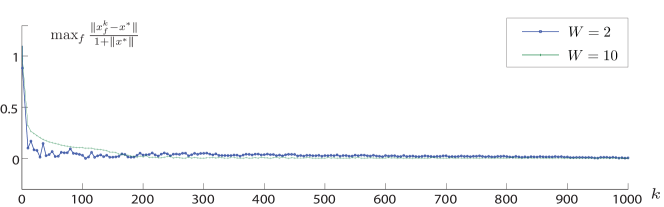
(a) Learning $x$

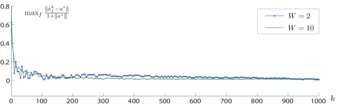
(b) Learning $a$

Figure 1: Computing $x^{*}$ and learning $a^{*}$ ($\xi\sim U[-{\theta}^{*}/2,{\theta}^{*}/2]$, $N=10$)

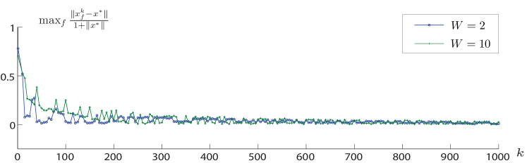
(a) Learning $x$

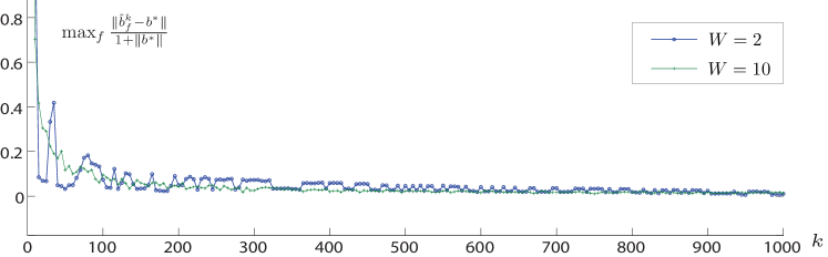
(b) Learning $b$

Figure 2: Computing $x^{*}$ and learning $b^{*}$ ( $\xi\sim U[-{\theta}^{*}/2,{\theta}^{*}/2]$, $N=10$)

TABLE III: Learning $x^{*}$ and $b^{*}$ in a stochastic regime when $N=5$ and $W=1$, stopping at step $k=10000$

	Sequential		Simultaneous
Bound	$\frac{\|x^{k}-x^{*}\|}{1+\|x^{*}\|}$	$\frac{\|\hat{b}^{k}-b^{*}\|}{1+\|b^{*}\|}$	$\frac{\max\|x_{f}^{k}-x^{*}\|}{1+\|x^{*}\|}$	$\frac{\max\|\hat{b}_{f}^{k}-b^{*}\|}{1+\|b^{*}\|}$
32.3664	2.1$\times 10^{-1}$	1.2$\times 10^{-1}$	4.9$\times 10^{-3}$	3.3$\times 10^{-3}$
64.7329	1.2$\times 10^{-1}$	1.0$\times 10^{-1}$	5.0$\times 10^{-3}$	3.3$\times 10^{-3}$
97.0993	5.5$\times 10^{-1}$	8.8$\times 10^{-1}$	5.0$\times 10^{-3}$	3.3$\times 10^{-3}$
129.4658	7.4$\times 10^{-1}$	1.1	5.1$\times 10^{-3}$	3.4$\times 10^{-3}$
161.8322	1.2	7.9$\times 10^{-1}$	5.1$\times 10^{-3}$	3.4$\times 10^{-3}$

(a) $\xi\sim U\textrm{[}-b^{*}/2,b^{*}/2\textrm{]}$

	Sequential		Simultaneous
$R$	$\frac{\|x^{k}-x^{*}\|}{1+\|x^{*}\|}$	$\frac{\|\hat{b}^{k}-b^{*}\|}{1+\|b^{*}\|}$	$\frac{\max\|x_{f}^{k}-x^{*}\|}{1+\|x^{*}\|}$	$\frac{\max\|\hat{b}_{f}^{k}-b^{*}\|}{1+\|b^{*}\|}$
$b^{*}/5$	7.5$\times 10^{-2}$	4.8$\times 10^{-2}$	1.9$\times 10^{-3}$	1.2$\times 10^{-3}$
$b^{*}/4$	9.6$\times 10^{-2}$	6.0$\times 10^{-2}$	2.4$\times 10^{-3}$	1.6$\times 10^{-3}$
$b^{*}/3$	1.3$\times 10^{-1}$	8.0$\times 10^{-2}$	3.2$\times 10^{-3}$	2.2$\times 10^{-3}$
$b^{*}/2$	2.1$\times 10^{-1}$	1.2$\times 10^{-1}$	4.9$\times 10^{-3}$	3.3$\times 10^{-3}$
$b^{*}/1$	5.3$\times 10^{-1}$	2.3$\times 10^{-1}$	9.9$\times 10^{-3}$	6.7$\times 10^{-3}$

(b) $\xi\sim U\textrm{[}-R,R\textrm{]}$

In Table IV(a), we raise the upper bounds of the strategy sets of all agents and compare a sequential scheme with our iterative fixed-point scheme. In the sequential counterpart, we employ $10,000$ steps of stochastic approximation-based learning followed by $10,000$ steps of computation. It is seen that the error from the sequential scheme increases proportionally to the bound, while the error associated with our simultaneous scheme does not change significantly. Table IV(b) shows that when increasing the variance of the noise makes the difference in errors between the sequential and simultaneous schemes more pronounced. Consequently, for the same effort, it can be seen that the simultaneous scheme performs far better to the sequential scheme, particularly when the variance of the noise grows.

V Concluding remarks

Nash games, a broadly applicable paradigm for modeling strategic interactions in noncooperative settings, have emerged as immensely useful in the context of distributed control problems. Yet, the development of distributed protocols for learning equilibria may be complicated by several challenges: (i) Agents may have an incomplete specification of payoffs; (ii) Agents may be unavailable to observe the actions of their counterparts; and finally, (iii) Observations may be corrupted by noise. Accordingly, this paper is motivated by developing schemes for learning equilibria and resolving misspecification (such as in the price functions). We consider two specific settings as part of our investigation and apply these techniques on a class of networked Nash-Cournot games. First, we consider convex static stochastic Nash games characterized by a suitable monotonicity property in which agent payoffs are parameterized by a misspecified vector. We consider a framework that combines (stochastic) gradient steps with a stochastic approximation step that attempts to learn the parameter. In such settings, we provide asymptotic statements that show that agents may learn equilibria and the true parameters in an almost sure sense. In addition, we provide non-asymptotic error bounds that demonstrate that the rate of convergence is not impaired by the presence of learning. Second, we refine our statements to a Cournot regime where we assume common knowledge holds but aggregate output is unobservable. In such a setting, we construct a learning scheme in which firms maintain a belief of the aggregate output and the misspecified price function parameter. After each step, these beliefs are updated by employ fixed-point steps and by leveraging the disparity between estimated and (noisy) observed prices. We proceed to show that in the limit, every firm learns the true Nash-Cournot equilibrium strategy in an almost-sure sense. Additionally, every firm learns the correct value of the misspecified parameter in an almost-sure sense. Yet much remains to be studied, including weakening monotonicity requirements on the map and boundedness requirements on the strategy sets. It also remains to be investigated as to whether learning can allow for weakening the common knowledge assumption.

Proof of Lemma 5: Since $x_{i}^{*}=\Pi_{K_{i}}(x_{i}^{*}-\gamma_{i}^{k}F_{i}(x^{*};\theta^{*}))$, by the nonexpansivity of the Euclidean projector:

$$\|x^{k+1}-x^{*}\|^{2} \leq\sum_{i=1}^{N}(\|x^{k}_{i}-x_{i}^{*}\|^{2}+(\gamma_{i}^{k})^{2}\|F_{i}(x^{k};\theta_{i}^{k})-F_{i}(x^{*};\theta^{*})\|^{2}+(\gamma_{i}^{k})^{2}\|w_{i}^{k}\|^{2})$$

$$-2\sum_{i=1}^{N}\gamma_{i}^{k}(x^{k}_{i}-x_{i}^{*})^{T}(F_{i}(x^{k};\theta_{i}^{k})-F_{i}(x^{*};\theta^{*}))$$

$$-2\sum_{i=1}^{N}\gamma_{i}^{k}(x^{k}_{i}-x_{i}^{*})^{T}w_{i}^{k}+2\sum_{i=1}^{N}(\gamma_{i}^{k})^{2}(F_{i}(x^{k};\theta_{i}^{k})-F_{i}(x^{*};\theta^{*}))^{T}w_{i}^{k}.$$ (24)

$$\mbox{RHS of }\eqref{eq:grad_dim}\leq\underbrace{\|x^{k}-x^{*}\|^{2}+(\gamma_{\max}^{k})^{2}\sum_{i=1}^{N}\|F_{i}(x^{k};\theta_{i}^{k})-F_{i}({\color[rgb]{0,0,0}{x^{*}}};\theta^{*})\|^{2}}_{\bf term\,1}+(\gamma_{\max}^{k})^{2}\|w^{k}\|^{2}$$

$$\quad\underbrace{-2\sum_{i=1}^{N}\gamma_{i}^{k}(x^{k}_{i}-x_{i}^{*})^{T}(F_{i}(x^{k};\theta_{i}^{k})-F_{i}(x^{k};\theta^{*}))}_{\bf term\,2}\ \,\underbrace{-2\sum_{i=1}^{N}\gamma_{i}^{k}(x^{k}_{i}-x_{i}^{*})^{T}(F_{i}(x^{k};\theta^{*})-F_{i}(x^{*};\theta^{*}))}_{\bf term\,3}$$

$$-2\sum_{i=1}^{N}\gamma_{i}^{k}(x^{k}_{i}-x_{i}^{*})^{T}w_{i}^{k}+2\sum_{i=1}^{N}(\gamma_{i}^{k})^{2}(F_{i}(x^{k};\theta_{i}^{k})-F_{i}(x^{*};\theta^{*}))^{T}w_{i}^{k}.$$ (25)

By (A1) and using inequality $\|a+b\|^{2}\leq 2\|a\|^{2}+2\|b\|^{2}$, term 1 in (Distributed computation of equilibria in misspecified convex stochastic Nash games) may be bounded by leveraging the Lipschitz continuity of $F(x;\theta)$:

$${\color[rgb]{0,0,0}{{\bf term\,1}}}\leq\|x^{k}-x^{*}\|^{2}+2(\gamma_{\max}^{k})^{2}\sum_{i=1}^{N}\|F_{i}(x^{k};\theta_{i}^{k})-F_{i}(x^{k};\theta^{*})\|^{2}+2(\gamma_{\max}^{k})^{2}\sum_{i=1}^{N}\|F_{i}(x^{k};\theta^{*})-F_{i}(x^{*};\theta^{*})\|^{2}$$

$$\leq\|x^{k}-x^{*}\|^{2}+2(\gamma_{\max}^{k})^{2}\sum_{i=1}^{N}\|F(x^{k};\theta_{i}^{k})-F(x^{k};\theta^{*})\|^{2}+2(\gamma_{\max}^{k})^{2}\|F(x^{k};\theta^{*})-F(x^{*};\theta^{*})\|^{2}$$

$$\leq(1+2(\gamma_{\max}^{k})^{2}L_{x}^{2})\|x^{k}-x^{*}\|^{2}+2(\gamma_{\max}^{k})^{2}L_{\theta}^{2}\sum_{i=1}^{N}\|\theta_{i}^{k}-\theta^{*}\|^{2}.$$ (26)

By (A1), term 2 in (Distributed computation of equilibria in misspecified convex stochastic Nash games) can be bounded by the Cauchy-Schwarz inequality, Hölder’s inequality and the Lipschitz continuity of $F(x;\theta)$:

$$\quad\ {\color[rgb]{0,0,0}{{\bf term\,2}}}$$

$$\leq-2\sum_{i=1}^{N}\gamma_{i}^{k}(x^{k}_{i}-x_{i}^{*})^{T}(F_{i}(x^{k};\theta_{i}^{k})-F_{i}(x^{k};\theta^{*}))\leq 2\gamma_{\max}^{k}\sum_{i=1}^{N}\|x_{i}^{k}-x_{i}^{*}\|\|F_{i}({x^{k}};\theta_{i}^{k})-F_{i}(x^{k};\theta^{*})\|$$

$$\leq 2\gamma_{\max}^{k}\|x^{k}-x^{*}\|\sqrt{\sum_{i=1}^{N}\|F_{i}(x^{k};\theta_{i}^{k})-F_{i}(x^{k};\theta^{*})\|^{2}}$$

$$\leq 2\gamma_{\max}^{k}\|x^{k}-x^{*}\|\sqrt{\sum_{i=1}^{N}\|F(x^{k};\theta_{i}^{k})-F(x^{k};\theta^{*})\|^{2}}$$

$$\leq 2\gamma_{\max}^{k}L_{\theta}\|x^{k}-x^{*}\|\sqrt{\sum_{i=1}^{N}\|\theta_{i}^{k}-\theta^{*}\|^{2}}\leq\gamma_{\max}^{k}\mu_{x}\|x^{k}-x^{*}\|^{2}+\gamma_{\max}^{k}\frac{L_{\theta}^{2}}{\mu_{x}}\sum_{i=1}^{N}\|\theta_{i}^{k}-\theta^{*}\|^{2},$$ (27)

where the last inequality follows from the fact that $2ab\leq a^{2}+b^{2}$. Term 3 in (Distributed computation of equilibria in misspecified convex stochastic Nash games) can be bounded by the Cauchy-Schwarz inequality and $\gamma_{i}^{k}\leq\gamma_{\max}^{k}$ for all $i$: ${\color[rgb]{0,0,0}{{\bf term\,3}\leq}}-2\sum_{i=1}^{N}\gamma_{i}^{k}(x^{k}_{i}-x_{i}^{*})^{T}(F_{i}(x^{k};\theta^{*})-F_{i}(x^{*};\theta^{*}))=-2\sum_{i=1}^{N}\gamma_{\max}^{k}(x^{k}_{i}-x_{i}^{*})^{T}(F_{i}(x^{k};\theta^{*})-F_{i}(x^{*};\theta^{*}))-2\sum_{i=1}^{N}(\gamma_{i}^{k}-\gamma_{\max}^{k})(x^{k}_{i}-x_{i}^{*})^{T}(F_{i}(x^{k};\theta^{*})-F_{i}(x^{*};\theta^{*}))\leq-2\gamma_{\max}^{k}\sum_{i=1}^{N}(x^{k}_{i}-x_{i}^{*})^{T}(F_{i}(x^{k};\theta^{*})-F_{i}(x^{*};\theta^{*}))+2(\gamma_{\max}^{k}-\gamma_{\min}^{k})\sum_{i=1}^{N}\|x_{i}^{k}-x_{i}^{*}\|\|F_{i}(x^{k};\theta^{*})-F_{i}(x^{*};\theta^{*})\|.$ Proceeding further, we may leverage Hölder’s inequality, the Lipschitz continuity of $F(x;\theta)$ and (A1) to obtain the following:

$$\quad-2\gamma_{\max}^{k}\sum_{i=1}^{N}(x^{k}_{i}-x_{i}^{*})^{T}(F_{i}(x^{k};\theta^{*})-F_{i}(x^{*};\theta^{*}))$$

$$+2(\gamma_{\max}^{k}-\gamma_{\min}^{k})\sum_{i=1}^{N}\|x_{i}^{k}-x_{i}^{*}\|\|F_{i}(x^{k};\theta^{*})-F_{i}(x^{*};\theta^{*})\|$$

$$\leq-2\gamma_{\max}^{k}(x^{k}-x^{*})^{T}(F(x^{k};\theta^{*})-F(x^{*};\theta^{*}))+2(\gamma_{\max}^{k}-\gamma_{\min}^{k})\|x^{k}-x^{*}\|\|F(x^{k};\theta^{*})-F(x^{*};\theta^{*})\|$$

$$\leq-2\gamma_{\max}^{k}\mu_{x}\|x^{k}-x^{*}\|^{2}+2(\gamma_{\max}^{k}-\gamma_{\min}^{k})L_{x}\|x^{k}-x^{*}\|^{2}.$$ (28)

Combining (24) with (Distributed computation of equilibria in misspecified convex stochastic Nash games), (Distributed computation of equilibria in misspecified convex stochastic Nash games), (Distributed computation of equilibria in misspecified convex stochastic Nash games), and (Distributed computation of equilibria in misspecified convex stochastic Nash games), we obtain

$$\|x^{k+1}-x^{*}\|^{2} \leq(1+2(\gamma_{\max}^{k})^{2}L_{x}^{2})\|x^{k}-x^{*}\|^{2}-\gamma_{\max}^{k}\mu_{x}\|x^{k}-x^{*}\|^{2}+2(\gamma_{\max}^{k}-\gamma_{\min}^{k})L_{x}\|x^{k}-x^{*}\|^{2}$$

$$+2(\gamma_{\max}^{k})^{2}L_{\theta}^{2}\sum_{i=1}^{N}\|\theta_{i}^{k}-\theta^{*}\|^{2}+\gamma_{\max}^{k}L_{\theta}^{2}/\mu_{x}\sum_{i=1}^{N}\|\theta_{i}^{k}-\theta^{*}\|^{2}+(\gamma_{\max}^{k})^{2}\|w^{k}\|^{2}$$

$$-2\sum_{i=1}^{N}\gamma_{i}^{k}(x^{k}_{i}-x_{i}^{*})^{T}w_{i}^{k}+2\sum_{i=1}^{N}(\gamma_{i}^{k})^{2}(F_{i}(x^{k};\theta_{i}^{k})-F_{i}(x^{*};\theta^{*}))^{T}w_{i}^{k}$$

$$=\left(1-\gamma_{\max}^{k}\mu_{x}+2(\gamma_{\max}^{k}-\gamma_{\min}^{k})L_{x}+2(\gamma_{\max}^{k})^{2}L_{x}^{2}\right)\|x^{k}-x^{*}\|^{2}$$

$$+(2(\gamma_{\max}^{k})^{2}L_{\theta}^{2}+\gamma_{\max}^{k}L_{\theta}^{2}/\mu_{x})\sum_{i=1}^{N}\|\theta_{i}^{k}-\theta^{*}\|^{2}+(\gamma_{\max}^{k})^{2}\|w^{k}\|^{2}$$

$$-2\sum_{i=1}^{N}\gamma_{i}^{k}(x^{k}_{i}-x_{i}^{*})^{T}w_{i}^{k}+2\sum_{i=1}^{N}(\gamma_{i}^{k})^{2}(F_{i}(x^{k};\theta_{i}^{k})-F_{i}(x^{*};\theta^{*}))^{T}w_{i}^{k}.$$

By taking conditional expectations and by recalling that $\mathbb{E}[{\color[rgb]{0,0,0}{w_{i}^{k}}}\mid{\mathcal{F}}_{k}]=0$ and $\mathbb{E}[\|{\color[rgb]{0,0,0}{w_{i}^{k}}}\|^{2}\mid{\mathcal{F}}_{k}]\leq\nu_{x}^{2}$, we obtain that $\mathbb{E}\left[\|x^{k+1}-x^{*}\|^{2}\mid\mathcal{F}_{k}\right]\leq\zeta_{k}\|x^{k}-x^{*}\|^{2}+\beta_{k}$, where $\zeta_{k}=1-\gamma_{\max}^{k}\mu_{x}+2(\gamma_{\max}^{k}-\gamma_{\min}^{k})L_{x}+2(\gamma_{\max}^{k})^{2}L_{x}^{2}$ and $\beta_{k}=(2(\gamma_{\max}^{k})^{2}L_{\theta}^{2}+\gamma_{\max}^{k}L_{\theta}^{2}/\mu_{x})\sum_{i=1}^{N}\|\theta_{i}^{k}-\theta^{*}\|^{2}+{\color[rgb]{0,0,0}{N}}(\gamma_{\max}^{k})^{2}\nu_{x}^{2}$.   

Proof of Theorem 1: From Lemma 5, the following holds for every $k$:

$$\begin{aligned} \mathbb{E}\left[\|x^{k+1}-x^{*}\|^{2}\mid\mathcal{F}_{k}\right]&\leq\underbrace{\left(1-\gamma_{\max}^{k}\mu_{x}+2(\gamma_{\max}^{k}-\gamma_{\min}^{k})L_{x}+2(\gamma_{\max}^{k})^{2}L_{x}^{2}\right)}_{\triangleq\,{\zeta_{k}}}\|x^{k}-x^{*}\|^{2}\\ &+\underbrace{(2(\gamma_{\max}^{k})^{2}L_{\theta}^{2}+\gamma_{\max}^{k}L_{\theta}^{2}/\mu_{x})\sum_{i=1}^{N}\|\theta_{i}^{k}-\theta^{*}\|^{2}+{\color[rgb]{0,0,0}{N}}(\gamma_{\max}^{k})^{2}\nu_{x}^{2}}_{\triangleq\,\beta_{k}}.\end{aligned}$$ (29)

By invoking the fixed-point property given by $\theta^{*}=\Pi_{\Theta}(\theta^{*}-\alpha_{i}^{k}\nabla_{\theta}g(\theta^{*}))$ (see [45]) and the non-expansivity of the Euclidean projector, we may derive the following bound on $\|\theta_{i}^{k+1}-\theta^{*}\|^{2}$:

$$\quad\ \|\theta_{i}^{k+1}-\theta^{*}\|^{2}\leq\|\theta_{i}^{k}-\theta_{i}^{*}-\alpha_{i}^{k}(\nabla_{\theta}g(\theta_{i}^{k})-\nabla_{\theta}g(\theta^{*}))-\alpha_{i}^{k}v_{i}^{k}\|^{2}$$

$$=\|\theta_{i}^{k}-\theta_{i}^{*}-\alpha_{i}^{k}(\nabla_{\theta}g(\theta_{i}^{k})-\nabla_{\theta}g(\theta^{*}))\|^{2}+(\alpha_{i}^{k})^{2}\|v_{i}^{k}\|^{2}-2{\color[rgb]{0,0,0}{\alpha_{i}^{k}}}(\theta_{i}^{k}-\theta_{i}^{*}-\alpha_{i}^{k}(\nabla_{\theta}g(\theta_{i}^{k})-\nabla_{\theta}g(\theta^{*})))^{T}v_{i}^{k}.$$

By taking conditional expectations, recalling that $\mathbb{E}[v_{i}^{k}\mid\mathcal{F}_{k}]=0$ and using Lemma 4, we obtain

$$\begin{aligned} \mathbb{E}[\|\theta_{i}^{k+1}-\theta^{*}\|^{2}\mid\mathcal{F}_{k}]&\leq\|\theta_{i}^{k}-\theta^{*}-\alpha_{i}^{k}(\nabla_{\theta}g(\theta_{i}^{k})-\nabla_{\theta}g(\theta^{*}))\|^{2}+(\alpha_{i}^{k})^{2}\mathbb{E}[\|v_{i}^{k}\|^{2}\mid\mathcal{F}_{k}]\\ &\leq(1-2\alpha_{i}^{k}\mu_{\theta}+(\alpha_{i}^{k})^{2}C_{\theta}^{2})\|\theta_{i}^{k}-\theta^{*}\|^{2}+(\alpha_{i}^{k})^{2}\nu_{\theta}^{2}\\ &\leq(1-2\alpha_{\min}^{k}\mu_{\theta}+(\alpha_{\max}^{k})^{2}C_{\theta}^{2})\|\theta_{i}^{k}-\theta^{*}\|^{2}+(\alpha_{\max}^{k})^{2}\nu_{\theta}^{2}.\end{aligned}$$ (30)

Next, by adding $\eqref{exp-bound-thm}$ and (30) and by invoking (A4), we obtain the following:

$$\quad\ \mathbb{E}\left[\|x^{k+1}-x^{*}\|^{2}\mid\mathcal{F}_{k}\right]+\mathbb{E}\left[\sum_{i=1}^{N}\|\theta^{k+1}_{i}-\theta^{*}\|^{2}\mid\mathcal{F}_{k}\right]$$

$$\leq\left(1-\gamma_{\max}^{k}\mu_{x}+2(\gamma_{\max}^{k}-\gamma_{\min}^{k})L_{x}+2(\gamma_{\max}^{k})^{2}L_{x}^{2}\right)\|x^{k}-x^{*}\|^{2}$$

$$+(1-2\alpha_{\min}^{k}\mu_{\theta}+(\alpha_{\max}^{k})^{2}C_{\theta}^{2}+2(\gamma_{\max}^{k})^{2}L_{\theta}^{2}+\gamma_{\max}^{k}L_{\theta}^{2}/\mu_{x})\sum_{i=1}^{N}\|\theta^{k}_{i}-\theta^{*}\|^{2}+{\color[rgb]{0,0,0}{N}}(\gamma_{\max}^{k})^{2}\nu_{x}^{2}+N(\alpha_{\max}^{k})^{2}\nu_{\theta}^{2}$$

$$\leq(1-\gamma_{\max}^{k}\mu_{x}+2(\gamma_{\max}^{k}-\gamma_{\min}^{k})L_{x}+2(\alpha_{\max}^{k})^{2}L_{x}^{2}\mu_{x}^{2}\mu_{\theta}^{2}/L_{\theta}^{4})\|x^{k}-x^{*}\|^{2}$$

$$+(1-\gamma_{\max}^{k}L_{\theta}^{2}/\mu_{x}+(\alpha_{\max}^{k})^{2}C_{\theta}^{2}+2(\alpha_{\max}^{k})^{2}\mu_{x}^{2}\mu_{\theta}^{2}/L_{\theta}^{2})\sum_{i=1}^{N}\|\theta^{k}_{i}-\theta^{*}\|^{2}+{\color[rgb]{0,0,0}{N}}(\gamma_{\max}^{k})^{2}\nu_{x}^{2}+N(\alpha_{\max}^{k})^{2}\nu_{\theta}^{2}$$

$$\leq\left(1-\upsilon_{k}\gamma_{\max}^{k}+\beta(\alpha_{\max}^{k})^{2}\right)\left(\|x^{k}-x^{*}\|^{2}+\sum_{i=1}^{N}\|\theta^{k}_{i}-\theta^{*}\|^{2}\right)+\delta_{k},$$

where the second inequality results from invoking A4(c) through which $-\mu_{\theta}\alpha^{k}_{\rm min}\leq-\gamma^{k}_{\max}L_{\theta}^{2}/\mu_{x}$ and $\upsilon_{k}=\min\{\mu_{x}-2(\gamma_{\max}^{k}-\gamma_{\min}^{k})L_{x}/\gamma_{\max}^{k},L_{\theta}^{2}/\mu_{x}\}$, $\beta=\max\{2L_{x}^{2}\mu_{x}^{2}\mu_{\theta}^{2}/L_{\theta}^{4},C_{\theta}^{2}+2\mu_{x}^{2}\mu_{\theta}^{2}/L_{\theta}^{2}\}$, and $\delta_{k}={\color[rgb]{0,0,0}{N}}(\gamma_{\max}^{k})^{2}\nu_{x}^{2}+N(\alpha_{\max}^{k})^{2}\nu_{\theta}^{2}$. To show the non-summability of $(\upsilon_{k}\gamma_{\max}^{k}-\beta({\color[rgb]{0,0,0}{\alpha}}_{\max}^{k})^{2})$, we consider two cases: (i) If $\mu_{x}\leq L_{\theta}^{2}/\mu_{x}$ then $\upsilon_{k}=\mu_{x}-2(\gamma_{\max}^{k}-\gamma_{\min}^{k})L_{x}/\gamma_{\max}^{k}$ and for some $K$, $\upsilon_{k}\geq\mu_{x}/2$ when $k>K$. Consequently, $\sum_{k>K}\upsilon_{k}\gamma_{\max}^{k}\geq\sum_{k>K}{\color[rgb]{0,0,0}{\mu_{x}\gamma_{\max}^{k}/2}}=\infty;$ (ii) Alternately, if $\mu_{x}>L_{\theta}^{2}/\mu_{x}$, then for some $K$, $\upsilon_{k}=L_{\theta}^{2}/\mu_{x}$ when $k>K$ and $\sum_{k>K}\upsilon_{k}\gamma_{\max}^{k}=\sum_{k>K}L_{\theta}^{2}/\mu_{x}\gamma_{\max}^{k}=\infty.$ Since ${\color[rgb]{0,0,0}{\alpha}}_{\max}^{k}$ is square summable from (A4), we conclude that $\sum_{k=0}^{\infty}(\upsilon_{k}\gamma_{\max}^{k}-\beta({\color[rgb]{0,0,0}{\alpha}}_{\max}^{k})^{2})=\infty.$ In addition, we have that

$$\lim_{k\to\infty}\frac{\delta_{k}}{{\upsilon_{k}}\gamma_{\max}^{k}-\beta({\color[rgb]{0,0,0}{\alpha}}_{\max}^{k})^{2}}=\lim_{k\to\infty}\frac{{\color[rgb]{0,0,0}{N}}(\gamma_{\max}^{k})^{2}\nu_{x}^{2}+N(\alpha_{\max}^{k})^{2}\nu_{\theta}^{2}}{{\upsilon_{k}}\gamma_{\max}^{k}-\beta({\color[rgb]{0,0,0}{\alpha}}_{\max}^{k})^{2}}=\lim_{k\to\infty}\frac{{\color[rgb]{0,0,0}{N}}(\gamma_{\max}^{k})\nu_{x}^{2}+N\frac{(\alpha_{\max}^{k})^{2}}{\gamma_{\max}^{k}}\nu_{\theta}^{2}}{{\upsilon_{k}}-\beta{\color[rgb]{0,0,0}{(\alpha_{\max}^{k})^{2}/\gamma_{\max}^{k}}}}=0,$$

where the last equality results from noting that $\lim_{k\to\infty}\gamma_{\max}^{k}=0$, $\lim_{k\to\infty}(\alpha_{\max}^{k})^{2}/\gamma_{\max}^{k}=0$ and $\lim_{k\to\infty}\upsilon_{k}=c>0.$ Then, by invoking the super-martingale convergence theorem (Lemma 2), we have that $\|x^{k}-x^{*}\|^{2}+\sum_{i=1}^{N}\|\theta_{i}^{k}-\theta^{*}\|^{2}\to 0$ $a.s.$ as $k\to\infty$, which implies that $x^{k}\to x^{*}$ and $\theta_{i}^{k}\to\theta^{*}$ $a.s.$ as $k\to\infty$ for all $i$.   

Proof of Theorem 2: Throughout this proof, $\lambda_{x,\min}\triangleq{\displaystyle\min_{1\leq i\leq N}}\{\lambda_{x,i}\}$, $\lambda_{x,\max}\triangleq{\displaystyle\max_{1\leq i\leq N}}\{\lambda_{x,i}\}$, $\lambda_{\theta,\min}\triangleq{\displaystyle\min_{1\leq i\leq N}}\{\lambda_{\theta,i}\}$, $\lambda_{\theta,\max}\triangleq{\displaystyle\max_{1\leq i\leq N}}\{\lambda_{\theta,i}\}$. Furthermore, $2\mu_{\theta}\lambda_{\theta,\min}>1$, $\mu_{x}\lambda_{x,\max}-2(\lambda_{x,\max}-\lambda_{x,\min})L_{x}>1$, $A_{k}\triangleq\frac{1}{2}\|x^{k}-x^{*}\|^{2}$, and $a_{k}\triangleq\mathbb{E}[A_{k}]$. Then, $A_{k+1}$ may be bounded as follows by using the non-expansivity of the Euclidean projector:

$$A_{k+1} =\frac{1}{2}\sum_{i=1}^{N}\|x_{i}^{k+1}-x_{i}^{*}\|^{2}=\frac{1}{2}\sum_{i=1}^{N}\|\Pi_{K_{i}}(x_{i}^{k}-\gamma_{i}^{k}\nabla_{x_{i}}f_{i}(x^{k};{\theta_{i}^{k}},\xi_{i}^{k}))-\Pi_{K_{i}}(x_{i}^{*})\|^{2}$$

$$\leq\frac{1}{2}\sum_{i=1}^{N}\|x_{i}^{k}-\gamma_{i}^{k}\nabla_{x_{i}}f_{i}(x^{k};{\theta_{i}^{k}},\xi_{i}^{k})-x_{i}^{*}\|^{2}\leq\frac{1}{2}\sum_{i=1}^{N}\|x_{i}^{k}-x_{i}^{*}-\gamma_{i}^{k}(F_{i}(x^{k};\theta_{i}^{k})+w_{i}^{k}))\|^{2}$$

$$=A_{k}+\frac{1}{2}\sum_{i=1}^{N}(\gamma_{i}^{k})^{2}\|F_{i}(x^{k};\theta_{i}^{k})+w_{i}^{k}\|^{2}-\sum_{i=1}^{N}\gamma_{i}^{k}(x_{i}^{k}-x_{i}^{*})^{T}(F_{i}(x^{k};\theta_{i}^{k})+w_{i}^{k}).$$ (31)

Note that $\mathbb{E}[(x_{i}^{k}-x_{i}^{*})^{T}w_{i}^{k}]{\color[rgb]{0,0,0}{=\mathbb{E}[\mathbb{E}[(w_{i}^{k})^{T}(x_{i}^{k}-x_{i}^{*})\mid{\mathcal{F}}_{k}]]}}=0$. By taking expectations on both sides of (Distributed computation of equilibria in misspecified convex stochastic Nash games) and by invoking the bounds $\mathbb{E}[\|F_{i}(x^{k};\theta_{i}^{k})+w_{i}^{k}\|^{2}]\leq M^{2}/N$ and $\mathbb{E}[\|\nabla_{\theta}g(\theta_{i}^{k})+v_{i}^{k}\|^{2}]\leq M_{\theta}^{2}$, it follows that

$$a_{k+1} \leq a_{k}+\frac{1}{2}(\gamma_{\max}^{k})^{2}M^{2}-\sum_{i=1}^{N}\gamma_{i}^{k}\mathbb{E}[(x_{i}^{k}-x_{i}^{*})^{T}F_{i}(x^{k};\theta_{i}^{k})].$$ (32)

By (Distributed computation of equilibria in misspecified convex stochastic Nash games) and (Distributed computation of equilibria in misspecified convex stochastic Nash games), the last term (including the negative sign) in (32) can be bounded by

$$\quad\ -\sum_{i=1}^{N}\gamma_{i}^{k}\mathbb{E}[(x_{i}^{k}-x_{i}^{*})^{T}(F_{i}(x^{k};\theta_{i}^{k})-F_{i}(x^{k};\theta^{*}))]$$

$$\quad\ -\sum_{i=1}^{N}\gamma_{i}^{k}\mathbb{E}[(x_{i}^{k}-x_{i}^{*})^{T}(F_{i}(x^{k};\theta^{*})-F_{i}(x^{*};\theta^{*}))]-\sum_{i=1}^{N}\gamma_{i}^{k}\mathbb{E}[(x_{i}^{k}-x_{i}^{*})^{T}F_{i}(x^{*};\theta^{*})]$$

$$\leq-\sum_{i=1}^{N}\gamma_{i}^{k}\mathbb{E}[(x_{i}^{k}-x_{i}^{*})^{T}(F_{i}(x^{k};\theta_{i}^{k})-F_{i}(x^{k};\theta^{*}))]-\sum_{i=1}^{N}\gamma_{i}^{k}\mathbb{E}[(x_{i}^{k}-x_{i}^{*})^{T}(F_{i}(x^{k};\theta^{*})-F_{i}(x^{*};\theta^{*}))]$$

$$\leq\gamma_{\max}^{k}\mu_{x}a_{k}+\gamma_{\max}^{k}L_{\theta}^{2}/(2\mu_{x})\sum_{i=1}^{N}\mathbb{E}[\|\theta_{i}^{k}-\theta^{*}\|^{2}]-2\gamma_{\max}^{k}\mu_{x}a_{k}+2(\gamma_{\max}^{k}-\gamma_{\min}^{k})L_{x}a_{k}.$$ (33)

Combining (32) and (Distributed computation of equilibria in misspecified convex stochastic Nash games), we get

$$a_{k+1} \leq(1-\gamma_{\max}^{k}\mu_{x}+2(\gamma_{\max}^{k}-\gamma_{\min}^{k})L_{x})a_{k}+\frac{1}{2}(\gamma_{\max}^{k})^{2}M^{2}+\gamma_{\max}^{k}L_{\theta}^{2}/(2\mu_{x})\sum_{i=1}^{N}\mathbb{E}[\|\theta_{i}^{k}-\theta^{*}\|^{2}].$$

Suppose $\alpha_{i}^{k}=\lambda_{\theta,i}/k$ for all $i$. Since the function $g(\theta)$ is strongly convex, we can use the standard rate estimate (cf. inequality (5.292) in [25]) to get the following

$$\mathbb{E}[\|\theta_{i}^{k}-\theta^{*}\|^{2}]\leq\frac{{\color[rgb]{0,0,0}{Q_{\theta}}}}{k},$$ (34)

where $Q_{\theta}\triangleq\max\{\lambda_{\theta,\max}^{2}M_{\theta}^{2}(2\mu_{\theta}\lambda_{\theta,\min}-1)^{-1}$, $\max_{i}\mathbb{E}[\|\theta_{i}^{0}-\theta^{*}\|^{2}]\}$ with $\lambda_{\theta,\min}>1/(2\mu_{\theta})$. Suppose $\gamma_{i}^{k}=\lambda_{x,i}/k$, allowing us to claim the following:

$$a_{k+1} \leq\left(1-\frac{\mu_{x}\lambda_{x,\max}-2(\lambda_{x,\max}-\lambda_{x,\min})L_{x}}{k}\right)a_{k}+\frac{\lambda_{x,\max}^{2}}{2k^{2}}\left(M^{2}+\frac{L_{\theta}^{2}N{\color[rgb]{0,0,0}{Q_{\theta}}}}{\lambda_{x,\max}\mu_{x}}\right),$$

By assuming that $\mu_{x}\lambda_{x,\max}-2(\lambda_{x,\max}-\lambda_{x,\min})L_{x}>1$, the result follows by observing that $\mathbb{E}[\|x^{k}-x^{*}\|^{2}]\leq\frac{{\color[rgb]{0,0,0}{Q_{x,{\theta}}}}}{k},$ where $Q_{x,{\theta}}\triangleq\max\left\{\frac{\lambda_{x,\max}^{2}M^{2}+\lambda_{x,\max}^{2}L^{2}_{\theta}NQ_{\theta}}{(\mu_{x}\lambda_{x,\max}-2(\lambda_{x,\max}-\lambda_{x,\min})L_{x}-1)},\mathbb{E}[\|x^{0}-x^{*}\|^{2}]\right\}.$   

Proof of Proposition 1: It suffices to show that given $p(X^{k};\theta^{*},\xi^{k})$ and $\{\bar{\vartheta}_{i}^{k}\}_{i=1}^{N}$, the variational inequality VI$({\cal Z},F^{k+1}{\color[rgb]{0,0,0}{+\epsilon^{k}\mathbf{I}}})$ has a unique solution for each $i$. Now, for simplicity, we ignore the superscript $k$ for all variables. Given $p$, $\bar{\vartheta}_{i}$, $i$ and $k$, let $H(z_{i})$ denote the Jacobian matrix $\nabla F(z_{i})$ of $F$ at $z_{i}\in\cal Z$. We will proceed to show that $H(z_{i})$ is a $\mathbf{P}$-matrix for all $z_{i}\in\cal\widetilde{Z}$ in part (a) and a $\mathbf{P_{0}}$-matrix for all $z_{i}\in\cal\widetilde{Z}$ in part (b) where $\cal Z\subset\cal\widetilde{Z}$ and $\cal\widetilde{Z}$ is a rectangle. Then, by invoking Proposition 3.5.9 in [45], the associated mapping $F$ is P-mapping on $\cal\widetilde{Z}$ in part (a) and a $\mathbf{P}_{0}$-mapping on $\cal\widetilde{Z}$ in part (b). Consequently, by Theorem 3.5.15 in [45], the regularized variational inequality VI$({\cal Z},F^{k+1}{\color[rgb]{0,0,0}{+\epsilon^{k}\mathbf{I}}})$ has a unique solution in both parts (a) and (b). Specifically, we employ a rectangular $\widetilde{\cal Z}$ defined as $\widetilde{\cal Z}\triangleq[0,\infty)^{N}\times\Theta,$ where $\Theta$ is a compact set in $(0,\infty)$. (a) Given $z_{i}\in\widetilde{\cal Z}$, let $H_{i}$ denote $H(z_{i})$. Then, $H_{i}=\left(\begin{array}[]{cc}A_{i}&B\\ C&D\end{array}\right)$, where $A_{i}=b^{*}(I+ee^{T})+E_{i}$, $B=-\frac{1}{k+1}e$, $C=-b^{*}e^{T}$, $D=\frac{1}{k+1}$, $e$ denotes the column of ones in $\mathbb{R}^{N}$, $E_{i}$ is an $N\times N$ diagonal matrix with $c_{j}^{\prime\prime}(x_{ij})$ as its $j$th diagonal entry. Since, the nonnegativity of $c_{j}^{\prime\prime}(x_{ij})$ follows from the convexity of costs, $E_{i}$ is a nonnegative diagonal matrix and is therefore positive semidefinite. Recall that the sum of a diagonal positive semidefinite matrix and a $\mathbf{P}$-matrix is a $\mathbf{P}$-matrix and it suffices to show that $H_{i}$ is a $\mathbf{P}$-matrix when $E_{i}=0$. This amounts to showing that the principal minors of $H$ are positive.

Since $A_{i}$ and $D$ are $\mathbf{P}$-matrices, we only consider the principal submatrix $H_{\alpha}$ of $H_{i}$, where $\alpha\subseteq\{1,\ldots,N\}$ is a nonempty index set and $H_{\alpha}$ is given by $H_{\alpha}\triangleq\left(\begin{array}[]{cccc}A_{\alpha}&B_{\alpha}\\ C_{\alpha}&D\end{array}\right),$ where $A_{\alpha}=b^{*}(I_{n_{\alpha}}+e^{n_{\alpha}}(e^{n_{\alpha}})^{T}),B_{\alpha}=-\frac{1}{k+1}e^{n_{\alpha}},C_{\alpha}=-b^{*}(e^{n_{\alpha}})^{T}$, and $I_{n_{\alpha}}$ and $e^{n_{\alpha}}$ denote the identity matrix and the column of ones in $\mathbb{R}^{n_{\alpha}\times n_{\alpha}}$ and $\mathbb{R}^{n_{\alpha}}$, respectively, with $n_{\alpha}=|\alpha|$. Since $A_{\alpha}^{-1}=\frac{1}{b^{*}}\left(I_{n_{\alpha}}-\frac{1}{n_{\alpha}+1}e^{n_{\alpha}}(e^{n_{\alpha}})^{T}\right)$, we have $C_{\alpha}A_{\alpha}^{-1}B_{\alpha}=\frac{1}{k+1}(e^{n_{\alpha}})^{T}\left(I_{n_{\alpha}}-\frac{1}{n_{\alpha}+1}e^{n_{\alpha}}(e^{n_{\alpha}})^{T}\right)e^{n_{\alpha}}$ $=\frac{1}{k+1}\left(n_{\alpha}-\frac{n_{\alpha}^{2}}{n_{\alpha}+1}\right)=\frac{1}{k+1}\left(\frac{n_{\alpha}}{n_{\alpha}+1}\right).$ It follows that $D-C_{\alpha}A_{\alpha}^{-1}B_{\alpha}=\frac{1}{k+1}-\frac{1}{k+1}\left(\frac{n_{\alpha}}{n_{\alpha}+1}\right)=\frac{1}{k+1}\left(\frac{1}{n_{\alpha}+1}\right)>0.$ Since $\det(A_{\alpha})>0$, we have $\det(H_{\alpha})=\det(A_{\alpha})\det\left(D-C_{\alpha}A_{\alpha}^{-1}B_{\alpha}\right)>0$ for all $\alpha\subseteq\{1,\ldots,N\}$ with $\alpha\neq\emptyset$. Therefore, $H$ is a $\mathbf{P}$-matrix.

(b) Analogous to our approach for (a), we consider a matrix $H_{i}$, given by $H_{i}=\nabla F(z_{i})$. Then, $H_{i}=\left(\begin{array}[]{cc}A_{i}&B_{i}\\ C_{i}&D_{i}\end{array}\right)$, where $A_{i}={\hat{b}}_{i}(I+ee^{T})+E_{i}$, $B_{i}=\frac{1}{k+1}({\color[rgb]{0,0,0}{\bf x}}_{i}+(e^{T}{\color[rgb]{0,0,0}{\bf x}}_{i})e)$, $C_{i}={\hat{b}}_{i}e^{T}$, and $D_{i}=\frac{1}{k+1}(e^{T}{\color[rgb]{0,0,0}{\bf x}}_{i})$, where ${\hat{b}}_{i}=\frac{1}{k+1}b_{i}+\frac{k}{k+1}{\bar{b\mkern 3.0mu}\mkern-3.0mu}{}_{i}$, ${\color[rgb]{0,0,0}{\bf x}}_{i}=(x_{i1},\ldots,x_{iN})^{T}$, $e$ denotes the column of ones in $\mathbb{R}^{N}$, and $E_{i}$ is an $N\times N$ diagonal matrix with $c_{j}^{\prime\prime}(x_{ij})$ as its $j$th diagonal entry. Recall that the sum of a diagonal positive semidefinite matrix and a $\mathbf{P}_{0}$-matrix is a $\mathbf{P}_{0}$-matrix. As in (a), it suffices to show that $H$ is a $\mathbf{P}_{0}$-matrix when $E_{i}=0$.

Since $A_{i}$ and $D_{i}$ are $\mathbf{P}_{0}$-matrices, we restrict our attention to the principal submatrix $H_{\alpha}$ of $H_{i}$, where $\alpha\subseteq\{1,\ldots,N\}$ is a nonempty index set, and $H_{\alpha}$ is given by $H_{\alpha}\triangleq\left(\begin{array}[]{cccc}A_{\alpha}&B_{\alpha}\\ C_{\alpha}&D_{i}\end{array}\right),$ where $A_{\alpha}={\hat{b}}_{i}(I_{n_{\alpha}}+e^{n_{\alpha}}(e^{n_{\alpha}})^{T}),B_{\alpha}=\frac{1}{k+1}({\color[rgb]{0,0,0}{\bf x}}_{\alpha}+(e^{T}x_{i})e^{n_{\alpha}}),C_{\alpha}={\hat{b}}_{i}(e^{n_{\alpha}})^{T},$ and $I_{n_{\alpha}}$ and $e^{n_{\alpha}}$ denote the identity matrix and the column of ones in $\mathbb{R}^{n_{\alpha}\times n_{\alpha}}$ and $\mathbb{R}^{n_{\alpha}}$, respectively, with $n_{\alpha}=|\alpha|$. Then, the following hold: (1) If ${\hat{b}}_{i}=0$, then $A_{\alpha}=0$ and $C_{\alpha}=0$, which implies $\det(H_{\alpha})=0$; (2) If ${\hat{b}}_{i}>0$, then $A_{\alpha}^{-1}=\frac{1}{{\hat{b}}_{i}}(I_{n_{\alpha}}-\frac{1}{n_{\alpha}+1}e^{n_{\alpha}}(e^{n_{\alpha}})^{T})$. So, we have

$$\quad\,C_{\alpha}A_{\alpha}^{-1}B_{\alpha}=\frac{1}{k+1}(e^{n_{\alpha}})^{T}\left(I_{n_{\alpha}}-\frac{1}{n_{\alpha}+1}e^{n_{\alpha}}(e^{n_{\alpha}})^{T}\right)(x_{\alpha}+(e^{T}x_{i})e^{n_{\alpha}})$$

$$=\frac{1}{k+1}((e^{n_{\alpha}})^{T}-\frac{n_{\alpha}}{n_{\alpha}+1}\left(e^{n_{\alpha}})^{T}\right)(x_{\alpha}+(e^{T}x_{i})e^{n_{\alpha}})=\frac{1}{(k+1)(n_{\alpha}+1)}\left((e^{n_{\alpha}})^{T}x_{\alpha}+n_{\alpha}(e^{T}x_{i})\right).$$

$$\implies D_{i}-C_{\alpha}A_{\alpha}^{-1}B_{\alpha} =\frac{1}{k+1}e^{T}x_{i}-\frac{1}{(k+1)(n_{\alpha}+1)}\left((e^{n_{\alpha}})^{T}x_{\alpha}+n_{\alpha}(e^{T}x_{i})\right)$$

$$=\frac{1}{(k+1)(n_{\alpha}+1)}\left(e^{T}x_{i}-(e^{n_{\alpha}})^{T}x_{\alpha}\right)\geq 0.$$

Since $\det(A_{\alpha})>0$, we have $\det(H_{\alpha})=\det(A_{\alpha})\det\left(D_{i}-C_{\alpha}A_{\alpha}^{-1}B_{\alpha}\right)\geq 0$.

Therefore, $\det(H_{\alpha})\geq 0$ for all nonempty $\alpha\subseteq\{1,\ldots,N\}$, implying that $H_{i}$ is a $\mathbf{P_{0}}$-matrix.  

Proof of Lemma 6: Let $g(x)=(c^{\prime}_{1}(x_{1}),\dots,c^{\prime}_{N}(x_{N}))^{T}$ and $e=(1,\ldots,1)^{T}$. Then, we have $F(x)=g(x)+b^{*}(x+Xe)-a^{*}e$, where $X=\sum_{i=1}^{N}x_{i}$. Note that $g(x)$ is monotone in $x$. Thus, we have for $x,y\in K$

$$(F(x)-F(y))^{T}(x-y) =(g(x)-g(y))^{T}(x-y)+b^{*}(x-y)^{T}(x-y)+b^{*}(X-Y)e^{T}(x-y)$$

$$\geq b^{*}(x-y)^{T}(x-y)+b^{*}(X-Y)^{T}(X-Y)\geq b^{*}\|x-y\|^{2}.$$

This implies that $F(x)$ is strongly monotone in $x$ with constant $b^{*}.$ Note that $g(x)$ is Lipschitz continuous on $K$ with constant $M$, where $M\triangleq\max_{i}\{M_{i}\}$. The Lipschitz continuity of $F(x)$ is easily shown:

$$\|F(x)-F(y)\| =\|g(x)-g(y)\|+b^{*}\|x-y\|+b^{*}\|(X-Y)e\|$$

$$\leq M\|x-y\|+b^{*}\|x-y\|+b^{*}\|ee^{T}\|\|x-y\|=L\|x-y\|,$$

where $L=M+b^{*}+b^{*}\|ee^{T}\|$. It follows that $F(x)$ is Lipschitz continuous with constant $L$.  

Proof of Proposition 2: From Lemma 6, the associated variational inequality VI$(K,F)$ has a strongly monotone mapping $F(x)$ over $K$. Consequently, VI$(K,F)$ admits a unique solution [45].   

Proof of Proposition 3: Consider $\theta_{1},\theta_{2}\in\Theta$ and let $F_{i}(\cdot):=F(\cdot,\theta_{i})$, $i=1,2$. Let $x_{i}$ be a solution of VI$(K,F_{i})$ for $i=1,2$. By the assumption of strong monotonicity on the map, we have that

$$(x_{1}-x_{2})^{T}(F_{1}(x_{1})-F_{1}(x_{2}))\geq c\|x_{2}-x_{1}\|^{2},$$ (35)

for some constant $c>0$ (assumed to be independent of $\theta_{1}$). Since $x_{1}$ is a solution of VI$(K,F_{1})$, it follows that $(x_{2}-x_{1})^{T}F_{1}(x_{1})\geq 0$, which together with (35) implies

$$(x_{2}-x_{1})^{T}F_{1}(x_{2})\geq c\|x_{2}-x_{1}\|^{2}.$$ (36)

We may express (36) as $(x_{2}-x_{1})^{T}(F_{1}(x_{2})-F_{2}(x_{2})+F_{2}(x_{2}))\geq c\|x_{2}-x_{1}\|^{2}.$ Now since $x_{2}$ is the solution of VI$(K,F_{2})$, it follows that $(x_{2}-x_{1})^{T}F_{2}(x_{2})\leq 0$. Consequently we obtain

$$\|x_{2}-x_{1}\|\|F_{1}(x_{2})-F_{2}(x_{2})\|\geq(x_{2}-x_{1})^{T}(F_{1}(x_{2})-F_{2}(x_{2}))\geq c\|x_{2}-x_{1}\|^{2}.$$ (37)

By Lipschitz continuity of $F(x,\theta)$ (assuming it is uniform in $x$), we have that $\|F_{1}(x_{2},\theta_{1})-F_{2}(x_{2},\theta_{2})\|\leq L_{\theta}\|\theta_{2}-\theta_{1}\|$, and hence by (37) $L_{\theta}\|x_{2}-x_{1}\|\|\theta_{2}-\theta_{1}\|\geq c\|x_{2}-x_{1}\|^{2}.$ It follows that $\|x_{2}-x_{1}\|\leq L_{\theta}c^{-1}\|\theta_{2}-\theta_{1}\|$.

To show (b), let $x(\theta_{i},\epsilon_{j})$ be the solution of VI$(K,G_{ij}(\cdot))$, where $G_{ij}(\cdot)=F(\cdot,\theta_{i})+\epsilon_{j}\mathbf{I}$. We begin by applying the triangle inequality to obtain that $\|x(\theta_{1},\epsilon_{1})-x(\theta_{2},\epsilon_{2})\|\leq\|x(\theta_{1},\epsilon_{1})-x(\theta_{2},\epsilon_{1})\|+\|x(\theta_{2},\epsilon_{1})-x(\theta_{2},\epsilon_{2})\|.$ Since $G_{i1}$ is strongly monotone in $x$ with constant $c+\epsilon_{1}$ and Lipschitz continuous in $\theta$ with constant $L_{\theta}$, respectively, we have that the first term is bounded by $L_{\theta}(c+\epsilon_{1})^{-1}\|\theta_{2}-\theta_{1}\|$ as a result from part (a). Before proceeding, the Lipschitz continuity of $F(x;\theta)+\epsilon I$ with respect to $\epsilon$ can be obtained as

$$\|(F(x;\theta)+\epsilon_{2}x)-(F(x;\theta)+\epsilon_{1}x)\|\leq\|x\|\|\epsilon_{1}-\epsilon_{2}\|\leq D\|\epsilon_{1}-\epsilon_{2}\|.$$

Since $G_{2j}$ is strongly monotone in $x$ with constant $c+\epsilon_{j}$ and Lipschitz continuous in $\epsilon$ with constant $D$, respectively, we have that the second term is bounded by $D(c+\epsilon_{1})^{-1}\|\epsilon_{2}-\epsilon_{1}\|$ as a result from part (a). Consequently, we obtain that

$$\|x(\theta_{1},\epsilon_{1})-x(\theta_{2},\epsilon_{2})\|\leq L_{\theta}(c+\epsilon_{1})^{-1}\|\theta_{2}-\theta_{1}\|+D(c+\epsilon_{1})^{-1}\|\epsilon_{2}-\epsilon_{1}\|.$$

The Lipschitz continuity of $x(\theta,\epsilon)$ with respect to its parameters follows.  

Proof of Theorem 3: Suppose $k\geq 0$. At the $k$th iteration, $\tilde{p}_{i}^{k}$ is a function of $\hat{\theta}_{i}^{k+1}$, which is a function of $\bar{\vartheta}_{i}^{k}$. Consequently, the fixed-point problem (15) is a function of $\bar{\vartheta}_{i}^{k}$. Since (15) has a unique solution (Prop. 1), it follows that $x_{i,\cdot}=x_{j,\cdot}$ for $i\neq j$ and $x_{ij}^{k}=x_{jj}^{k}$. Therefore, Given $p(X^{k};\theta^{*},\xi^{k})$ and $\{\bar{\vartheta}_{i}^{k}\}_{i=1}^{N}$,the solution $({\color[rgb]{0,0,0}{\bf x}}_{i}^{k+1},\theta_{i}^{k+1})$ to (15) satisfies $x_{ij}^{k+1}=x_{jj}^{k+1}$ for all $i,j$. Thus, for all $k\geq 0$ and all $i$, we have that

$$p(X^{k};{\color[rgb]{0,0,0}{\theta^{*}}},\xi^{k})=\begin{cases}(a^{*}+\xi^{k})-b^{*}\sum_{j=1}^{N}x_{jj}^{k}=(a^{*}+\xi^{k})-b^{*}\sum_{j=1}^{N}x_{ij}^{k},&\quad\mbox{under }~{}\textbf{(A\ref{assump:ab}a)},\\ a^{*}-(\theta^{*}+\xi^{k})\sum_{j=1}^{N}x_{jj}^{k}=a^{*}-(\theta^{*}+\xi^{k})\sum_{j=1}^{N}x_{ij}^{k},&\quad\mbox{under }~{}\textbf{(A\ref{assump:ab}b)}.\end{cases}$$

Since for all $k\geq 0$ and all $i$,

$$\vartheta_{i}^{k}=\begin{cases}p(X^{k};{\color[rgb]{0,0,0}{\theta^{*}}},\xi^{k})+b^{*}X_{i}^{k},&\quad\mbox{under }~{}\textbf{(A\ref{assump:ab}a)},\\ (a^{*}-p(X^{k};{\color[rgb]{0,0,0}{\theta^{*}}},\xi^{k}))/X_{i}^{k},&\quad\mbox{under }~{}\textbf{(A\ref{assump:ab}b)}.\end{cases}$$

we have $\vartheta_{i}^{k}=\theta^{*}+\xi^{k}$ for all $i$. As a result, after $k$ iterative fixed-point steps, we obtain $k$ samples $\{\theta^{*}+\xi^{1},\ldots,\theta^{*}+\xi^{k}\}$ of the estimated parameter. Since for all $k\geq 0$ and all $i$, ${\color[rgb]{0,0,0}{\bar{\vartheta}_{i}^{k+1}=\frac{k\bar{\vartheta}_{i}^{k}+\vartheta_{i}^{k+1}}{k+1}}}$, the sample mean of the estimated parameter is given by $\bar{\vartheta}_{i}^{k}$, i.e.,

$$\bar{\vartheta}_{i}^{k}=\frac{\sum_{l=1}^{k}(\theta^{*}+\xi^{l})}{{k}}.$$ (38)

Therefore, $\bar{\vartheta}_{i}^{k}\to\theta^{*}$ $a.s.$ as $k\to\infty$, which implies by the boundedness of $\{\theta_{i}^{k}\}$ that for all $i$

$${\widehat{\theta}}_{i}^{k+1}=\frac{1}{k+1}\theta_{i}^{k+1}+\frac{k}{k+1}\bar{\vartheta}_{i}^{k}\to\theta^{*}\quad\,\textrm{{a.s.}\,\, as }k\to\infty,$$

by the strong law of large numbers. By Proposition 3, ${\color[rgb]{0,0,0}{\bf x}}^{k+1}_{i}=x^{k+1}_{i}({\widehat{\theta}}_{i}^{k+1},\epsilon^{k})$ is a continuous function of $({\widehat{\theta}}_{i}^{k+1},\epsilon^{k})$, and ${\color[rgb]{0,0,0}{\bf x}}^{k+1}_{i}(\theta^{*},0)=x^{*}$. Therefore, ${\color[rgb]{0,0,0}{\bf x}}^{k+1}_{i}\to x^{*}$ $a.s.$ as $k\to\infty$.   

Proof of Lemma 7: (a) Strict monotonicity of $F(x)$ is implied by the positive definiteness of the Jacobian $\nabla F(x).$ This is given by $\nabla F(x)=J_{1}+J_{2}+J_{3}$, where $J_{2}=2b^{*}\sigma X^{\sigma-1}ee^{T}$ and $J_{1}=\begin{pmatrix}c_{1}^{\prime\prime}(x_{1})&\\ &\ddots\\ &&c_{N}^{\prime\prime}(x_{N})\end{pmatrix}\mbox{ and },J_{3}=b^{*}\sigma(\sigma-1)X^{\sigma-2}\begin{pmatrix}\frac{X}{\sigma-1}+x_{1}&\ldots&x_{1}\\ \vdots&\ddots&\vdots\\ x_{N}&\ldots&\frac{X}{\sigma-1}+x_{N}\end{pmatrix}.$ Since $c_{i}(x_{i})$ is a convex function in $x_{i}$ for all $i$, $J_{1}$ is a positive semidefinite matrix. $J_{2}$, compactly stated as $2b^{*}\sigma X^{\sigma-1}ee^{T}$, is also a positive semidefinite matrix. As a consequence, positive definiteness of $\nabla F(x)$ follows from the diagonal dominance of the following matrix:

$$b^{*}\sigma(\sigma-1)X^{\sigma-2}\begin{pmatrix}\frac{X}{\sigma-1}+x_{1}&\ldots&{1\over 2}(x_{1}+x_{N})\\ \vdots&\ddots&\vdots\\ {1\over 2}(x_{N}+x_{1})&\ldots&\frac{X}{\sigma-1}+x_{N}\end{pmatrix}.$$

By a minor rearrangement, it suffices to show the diagonal dominance of the following:

$$b^{*}\sigma(\sigma-1)X^{\sigma-2}\begin{pmatrix}\frac{X_{-1}}{\sigma-1}+(1+\frac{1}{(\sigma-1)})x_{1}&\ldots&{1\over 2}(x_{1}+x_{N})\\ \vdots&\ddots&\vdots\\ {1\over 2}(x_{N}+x_{1})&\ldots&\frac{X_{-N}}{\sigma-1}+(1+\frac{1}{(\sigma-1)})x_{N}\end{pmatrix},$$

where $X_{-j}\triangleq\sum_{i\neq j}x_{i}$. The result follows by noting that

$$\left(1+\frac{1}{(\sigma-1)}\right)>\frac{(N-1)}{2}\mbox{ or }\frac{2\sigma}{\sigma-1}>N-1\mbox{ or }N<\frac{3\sigma-1}{\sigma-1},$$

and $\frac{1}{(\sigma-1)}\geq\frac{1}{2}\mbox{ or }1<\sigma\leq 3.$ (b) For $x,y\in K$, $(x-y)^{T}(F(x)-F(y))=\int_{0}^{1}(x-y)^{T}\nabla F(y+\alpha(x-y))(x-y)d\alpha.$ Let $\tilde{x}=y+\alpha(x-y)$ an $\tilde{X}=\sum_{i=1}^{N}{\tilde{x}_{i}}$. Akin to $\nabla F(x)$, $\nabla F(y+\alpha(x-y))=\tilde{J}_{1}+\tilde{J}_{2}+\tilde{J}_{3}$, where $\tilde{J}_{1}$ and $\tilde{J}_{2}$ are positive semidefinite, and $\tilde{J}_{3}=b^{*}\sigma(\sigma-1)\tilde{X}^{\sigma-2}\tilde{J}_{4}$, where

$$\tilde{J}_{4} =\begin{pmatrix}\frac{\tilde{X}_{-1}}{\sigma-1}+(1+\frac{1}{(\sigma-1)})\tilde{x}_{1}&\ldots&{1\over 2}(\tilde{x}_{1}+\tilde{x}_{N})\\ \vdots&\ddots&\vdots\\ {1\over 2}(\tilde{x}_{N}+\tilde{x}_{1})&\ldots&\frac{\tilde{X}_{-N}}{\sigma-1}+(1+\frac{1}{(\sigma-1)})\tilde{x}_{N}\end{pmatrix}$$

$$=\begin{pmatrix}\frac{\tilde{X}_{-1}}{\sigma-1}+\frac{N-1}{2}\tilde{x}_{1}&\ldots&{1\over 2}(\tilde{x}_{1}+\tilde{x}_{N})\\ \vdots&\ddots&\vdots\\ {1\over 2}(\tilde{x}_{N}+\tilde{x}_{1})&\ldots&\frac{\tilde{X}_{-N}}{\sigma-1}+\frac{N-1}{2}\tilde{x}_{N}\end{pmatrix}+\left(\frac{\sigma}{\sigma-1}-\frac{N-1}{2}\right)I_{N}\triangleq\tilde{J}_{5}+\rho I_{N},$$

where $\tilde{J}_{5}$ is a positive semidefinite matrix and $\rho=(1+\frac{1}{\sigma-1}-\frac{N-1}{2})>0$. Therefore,

$$\quad(x-y)^{T}(F(x)-F(y))\geq\int_{0}^{1}(x-y)^{T}\tilde{J}_{3}(x-y)d\alpha\geq b^{*}\sigma(\sigma-1)\int_{0}^{1}(x-y)^{T}\tilde{X}^{\sigma-2}\tilde{J}_{4}(x-y)d\alpha$$

$$\geq b^{*}\sigma(\sigma-1)\eta^{\sigma-2}\int_{0}^{1}(x-y)^{T}(\tilde{J}_{5}+\rho I_{N})(x-y)d\alpha\geq b^{*}\sigma(\sigma-1)\eta^{\sigma-2}\rho\|x-y\|^{2},$$

implying the strong monotonicity of $F$.  

Proof of Corollary 1: By Proposition 3, it suffices to show that $F(x;\theta)$ is Lipschitz continuous in $x$ for all $\theta\in\Theta$. For $\theta\in\Theta$, and $x,y\in K$, we have that

$$\|F(x;\theta)-F(y;\theta)\| =\left\|\int_{0}^{1}\nabla F(y+\alpha(x-y);\theta)(x-y)d\alpha\right\|\quad\textrm{for some }\alpha\in(0,1)$$

$$\leq\int_{0}^{1}\left\|\nabla F(y+\alpha(x-y);\theta)\right\|\|x-y\|d\alpha\leq\int_{0}^{1}r\|x-y\|d\alpha=r\|x-y\|,$$

which implies the Lipschitz continuity in $x$ of the mapping $F$.   

Proof of Proposition 4: By Lemma 7, $F(x;\theta)$ is a strongly monotone mapping over $K$ for all $\theta\in\Theta$. By definition of $F$, $F(x;\theta)$ is Lipschitz continuous in $\theta$ for all $x\in K$. By definition of $\nabla F$ and boundedness of $x\in K$, $\nabla F(x;\theta)$ is bounded for $x\in K$ and $\theta\in\Theta$. Then, the conclusion follows from Corollary 1.   

Proof of Proposition 5: Given $p$, $\bar{\theta}_{i}$, $i$ and $k$, let $H(z_{i})$ denote the Jacobian matrix $\nabla F(z_{i})$ of the mapping $F$ at $z_{i}\in\widetilde{\cal Z}$. Then, as in Proposition 1, it suffices to show that $H(z_{i})$ is a $\mathbf{P}$-matrix for all $z_{i}\in\widetilde{\cal Z}$. Given $z_{i}\in\widetilde{\cal Z}$, let $H=H(z_{i})$. Then, $H=H(z_{i})=\left(\begin{array}[]{cc}A_{i}&B\\ C_{i}&D\end{array}\right)$, where $A_{i}=\sigma b^{*}(X_{i})^{\sigma-2}\left[X_{i}(I+ee^{T})+(\sigma-1){\color[rgb]{0,0,0}{\bf x}}_{i}e^{T}\right]+E_{i}$, $B=-\frac{1}{k+1}e$, $C_{i}=-\sigma b^{*}(X_{i})^{\sigma-1}e^{T}$, and $D=\frac{1}{k+1}$, where $X_{i}=\sum_{j=1}^{N}x_{ij}$, ${\color[rgb]{0,0,0}{\bf x}}_{i}=(x_{11},\ldots,x_{1N})^{T}$, and $E_{i}$ is an $N\times N$ diagonal matrix with $c_{j}^{\prime\prime}(x_{ij})$ as its $j$th diagonal entry. It suffices to show that $H$ is a $\mathbf{P}$-matrix when $E_{i}=0$.

If $N<\frac{3\sigma-1}{\sigma-1}$, then $A_{i}$ is positive semidefinite by Lemma 7. Therefore, we only consider the principal submatrix $H_{\alpha}$ of $H$, where $\alpha\subseteq\{1,\ldots,N\}$ is a nonempty index set, and $H_{\alpha}\triangleq\left(\begin{array}[]{cccc}A_{\alpha}&B_{\alpha}\\ C_{\alpha}&D\end{array}\right),$ where $A_{\alpha}=\sigma b^{*}(X_{i})^{\sigma-1}\left[I_{n_{\alpha}}+e^{n_{\alpha}}(e^{n_{\alpha}})^{T}\right]+\sigma(\sigma-1)b^{*}(X_{i})^{\sigma-2}{\color[rgb]{0,0,0}{\bf x}}_{\alpha}(e^{n_{\alpha}})^{T},B_{\alpha}=-\frac{1}{k+1}e^{n_{\alpha}},C_{\alpha}=-\sigma b^{*}(X_{i})^{\sigma-1}(e^{n_{\alpha}})^{T},$ and $I_{n_{\alpha}}$ and $e^{n_{\alpha}}$ denote the identity matrix and the column of ones in $\mathbb{R}^{n_{\alpha}\times n_{\alpha}}$ and $\mathbb{R}^{n_{\alpha}}$, respectively, with $n_{\alpha}=|\alpha|$. Since

$$B_{\alpha}D^{-1}C_{\alpha} =\frac{1}{k+1}e^{n_{\alpha}}(k+1)\sigma b^{*}(X_{i})^{\sigma-1}(e^{n_{\alpha}})^{T}=\sigma b^{*}(X_{i})^{\sigma-1}e^{n_{\alpha}}(e^{n_{\alpha}})^{T},$$

it follows that $A_{\alpha}-B_{\alpha}D^{-1}C_{\alpha}=\sigma b^{*}(X_{i})^{\sigma-1}I_{n_{\alpha}}+\sigma(\sigma-1)b^{*}(X_{i})^{\sigma-2}{\color[rgb]{0,0,0}{\bf x}}_{\alpha}(e^{n_{\alpha}})^{T},$ which is a sum of a diagonal positive definite matrix and a $\mathbf{P_{0}}$-matrix, and thus is a $\mathbf{P}$-matrix. Therefore, $\det(H_{\alpha})=\det(D)\det(A_{\alpha}-B_{\alpha}D^{-1}C_{\alpha})>0$ for all $\alpha\subseteq\{1,\ldots,N\}$ with $\alpha\neq\emptyset$, which implies that $H$ is a $\mathbf{P}$-matrix.

References

[1]
H. Jiang, U. V. Shanbhag, and S. P. Meyn, “Learning equilibria in constrained
Nash-Cournot games with misspecified demand functions,” in
Proceedings of the IEEE Conference on Decision and Control (CDC-ECE),
2011, pp. 1018–1023.
[2]
J. R. Marden and J. S. Shamma, “Game theory and distributed control,” H. P.
Young and S. Zamir, Eds., vol. 4. Elsevier, 2014.
[3]
N. Li and J. R. Marden, “Designing games to handle coupled constraints,” in
Proceedings of the IEEE Conference on Decision and Control
(CDC). IEEE, 2010, pp. 250–255.
[4]
——, “Designing games for distributed optimization,” in Proceedings
of the IEEE Conference on Decision and Control (CDC), 2011, pp. 2434–2440.
[5]
D. Fudenberg and D. K. Levine, The theory of learning in games, ser. MIT
Press Series on Economic Learning and Social Evolution. Cambridge, MA: MIT Press, 1998, vol. 2.
[6]
H. P. Young, Strategic Learning and its Limits. Oxford University Press, 2004.
[7]
S. Hart, “Adaptive heuristics,” Econometrica, vol. 73, no. 5, pp.
1401–1430, 2005.
[8]
J. S. Shamma and G. Arslan, “Dynamic fictitious play, dynamic gradient play,
and distributed convergence to Nash equilibria,” IEEE Trans.
Automat. Control, vol. 50, no. 3, pp. 312–327, 2005.
[9]
T. Başar, “Control and game-theoretic tools for communication
networks,” Appl. Comput. Math., vol. 6, no. 2, pp. 104–125, 2007.
[10]
T. Alpcan and T. Başar, “Distributed algorithms for Nash equilibria of
flow control games,” Annals of Dynamic Games, vol. 7, 2003.
[11]
Y. Pan and L. Pavel, “Games with coupled propagated constraints in optical
network with multi-link topologies,” Automatica, vol. 45, pp.
871–880, 2009.
[12]
H. Yin, U. V. Shanbhag, and P. G. Mehta, “Nash equilibrium problems with
scaled congestion costs and shared constraints,” IEEE Transactions on
Automatic Control, vol. 56, no. 7, pp. 1702–1708, 2011.
[13]
F. Facchinei and J. S. Pang, “Nash Equilibria: The Variational Approach,”
Convex Optimization in Signal Processing and Communication, Cambridge
University Press, 2009.
[14]
G. Scutari and J.-S. Pang, “Joint sensing and power allocation in nonconvex
cognitive radio games: Quasi-Nash equilibria,” in Digital Signal
Processing (DSP), 2011 17th International Conference on. IEEE, 2011, pp. 1–8.
[15]
A. P. Kirman, “Learning by firms about demand conditions,” in Adaptive
economic models (Proc. Sympos., Math. Res. Center, Univ.
Wisconsin, Madison, Wis., 1974). New York: Academic Press, 1975, pp. 137–156. Math. Res. Center,
Univ. Wisconsin, Publ. No. 34.
[16]
G. I. Bischi, A. Naimzada, and L. Sbragia, “Oligopoly games with local
monopolistic approximation,” Journal of Economic Behavior and
Organization, vol. 62, pp. 371–388, 2007.
[17]
G. I. Bischi, L. Sbragia, and F. Szidarovszky, “Learning the demand function
in a repeated Cournot oligopoly game,” Internat. J. Systems Sci.,
vol. 39, no. 4, pp. 403–419, 2008.
[18]
F. Szidarovszky, “Global stability analysis of a special learning process in
dynamic oligopolies,” Journal of Economic and Social Research,
vol. 9, pp. 175–190, 2004.
[19]
F. Szidarovszky and J. B. Krawczyk, “On stable learning in dynamic
oligopolies,” Pure Math. Appl., vol. 15, no. 4, pp. 453–468, 2004.
[20]
D. Léonard and K. Nishimura, “Nonlinear dynamics in the Cournot model
without full information,” Ann. Oper. Res., vol. 89, pp. 165–173,
1999, nonlinear dynamical systems and adaptive methods (Vienna, 1997).
[21]
W. L. Cooper, T. Homem-de Mello, and A. J. Kleywegt, “Models of the
spiral-down effect in revenue management,” Oper. Res., vol. 54, pp.
968–987, September 2006.
[22]
B. F. Hobbs, “Linear complementarity models of Nash-Cournot competition in
bilateral and poolco power markets,” IEEE Transactions on Power
Systems, vol. 16, no. 2, pp. 194–202, 2001.
[23]
B. F. Hobbs and J. S. Pang, “Nash-Cournot equilibria in electric power
markets with piecewise linear demand functions and joint constraints,”
Oper. Res., vol. 55, no. 1, pp. 113–127, 2007.
[24]
L. Pavel, “A noncooperative game approach to OSNR optimization in optical
networks,” IEEE Trans. Automat. Control, vol. 51, no. 5, pp.
848–852, 2006.
[25]
A. Shapiro, D. Dentcheva, and A. Ruszczyński, Lectures on stochastic
programming, ser. MPS/SIAM Series on Optimization. Philadelphia, PA: SIAM, 2009, vol. 9, modeling and theory.
[Online]. Available: http://dx.doi.org/10.1137/1.9780898718751
[26]
T. Hastie, R. Tibshirani, and J. H. Friedman, The elements of statistical
learning: data mining, inference, and prediction: with 200 full-color
illustrations. New York:
Springer-Verlag, 2001.
[27]
C. H. Papadimitriou and M. Yannakakis, “On bounded rationality and
computational complexity,” Indiana University, Tech. Rep., 1994.
[28]
H. A. Simon, The sciences of the artificial (3rd ed.). Cambridge, MA, USA: MIT Press, 1996.
[29]
H. Jiang and U. V. Shanbhag, “On the solution of stochastic optimization
problems in imperfect information regimes,” in Winter Simulation
Conference: Simulation Making Decisions in a Complex World, WSC 2013,
Washington, DC, USA, December 8-11, 2013. IEEE, 2013, pp. 821–832. [Online]. Available:
http://dx.doi.org/10.1109/WSC.2013.6721474
[30]
——, “On the solution of stochastic optimization and variational problems
in imperfect information regimes,” SIAM Journal on Optimization,
vol. 26, no. 4, pp. 2394–2429, 2016. [Online]. Available:
https://doi.org/10.1137/140955495
[31]
V. S. Borkar, Stochastic Approximation: A Dynamical Systems
Viewpoint. Cambridge University
Press, 2008.
[32]
B. T. Polyak and A. B. Juditsky, “Acceleration of stochastic approximation by
averaging,” SIAM J. Control Optim., vol. 30, no. 4, pp. 838–855,
1992. [Online]. Available: http://dx.doi.org/10.1137/0330046
[33]
H. J. Kushner and G. G. Yin, Stochastic approximation and recursive
algorithms and applications, 2nd ed., ser. Applications of Mathematics (New
York). New York: Springer-Verlag,
2003, vol. 35, stochastic Modelling and Applied Probability.
[34]
J. Hofbauer and W. H. Sandholm, “Stable games and their dynamics,” J.
Economic Theory, vol. 144, no. 4, pp. 1665–1693, 2009.
[35]
M. J. Fox and J. S. Shamma, “Population games, stable games, and passivity,”
in CDC, 2012, pp. 7445–7450.
[36]
A. Kannan and U. V. Shanbhag, “Distributed computation of equilibria in
monotone Nash games via iterative regularization techniques,” SIAM
Journal of Optimization, vol. 22, no. 4, pp. 1177–1205, 2012.
[37]
B. T. Polyak, Introduction to optimization. New York: Optimization Software, Inc., 1987.
[38]
F. Facchinei and J. S. Pang, Finite-dimensional variational inequalities
and complementarity problems. Vol. II, ser. Springer Series in
Operations Research. New York:
Springer-Verlag, 2003.
[39]
A. Juditsky, A. Nemirovski, and C. Tauvel, “Solving variational inequalities
with stochastic mirror-prox algorithm,” Stoch. Syst., vol. 1, no. 1,
pp. 17–58, 2011. [Online]. Available:
http://dx.doi.org/10.1214/10-SSY011
[40]
G. I. Bischi, C. Chiarella, M. Kopel, and F. Szidarovszky, Nonlinear
oligopolies. Berlin: Springer-Verlag,
2010, stability and bifurcations.
[41]
R. J. Aumann, “Agreeing to disagree,” The Annals of Statistics,
vol. 4, no. 6, pp. pp. 1236–1239, 1976.
[42]
J. Littlewood, Mathematical Miscellany, B. Bollabos, Ed., 1953.
[43]
T. Shelling, The Strategy of Conflict. Harvard University Press, Cambridge, Massachusetts, 1960.
[45]
F. Facchinei and J. S. Pang, Finite-dimensional variational inequalities
and complementarity problems. Vol. I, ser. Springer Series in Operations
Research. New York: Springer-Verlag,
2003.
[46]
S. Dafermos, “Sensitivity analysis in variational inequalities,” Math.
Oper. Res., vol. 13, no. 3, pp. 421–434, 1988.
[47]
T. W. Anderson and J. B. Taylor, “Strong consistency of least squares
estimates in dynamic models,” The Annals of Statistics, vol. 7,
no. 3, pp. 484–489, 1979.
[48]
M. C. Ferris and T. S. Munson, “Complementarity problems in gams and the path
solver,” Journal of Economic Dynamics and Control, vol. 24, no. 2,
pp. 165–188, 2000.