COAST: A Convex Optimization Approach
to Stress-Based Embedding

Abstract

Visualizing graphs using virtual physical models is probably the most heavily used technique for drawing graphs in practice. There are many algorithms that are efficient and produce high-quality layouts. If one requires that the layout also respect a given set of non-uniform edge lengths, however, force-based approaches become problematic while energy-based layouts become intractable. In this paper, we propose a reformulation of the stress function into a two-part convex objective function to which we can apply semi-definite programming (SDP). We avoid the high computational cost associated with SDP by a novel, compact re-parameterization of the objective function using the eigenvectors of the graph Laplacian. This sparse representation makes our approach scalable. We provide experimental results to show that this method scales well and produces reasonable layouts while dealing with the edge length constraints.

1 Introduction

For visualizing general undirected graphs, algorithms based on virtual physical models are some of the most frequently used drawing methods. Among these, the spring-electrical model [7, 8] treats edges as springs that pull nodes together, and nodes as electrically-charged entities that repel each other. Efficient and effective implementations [12, 13, 25] usually utilize a multilevel approach and fast force approximation with a suitable spatial data structure, and can scale to millions of vertices and edges while still producing high-quality layouts.

In certain instances, the graph may assign non-uniform lengths to its edges, and the layout problem will have the additional constraint of trying to match these lengths. A suitable formulation of the spring-electrical model that works well when edges have predefined target lengths is still an open problem.

In contrast, the (full) stress model assumes that there are springs connecting all vertex pairs of the graph. Assuming we have a graph $G=(V,E)$, with $V$ the set of vertices and $E$ the set of edges, the energy of this spring system is

$$\sum_{i,j\in V}w_{{ij}}\left(\left\|x_{i}-x_{j}\right\|-d_{{ij}}\right){}^{2},$$ (1)

where $d_{ij}$ is the ideal distance between vertices $i$ and $j$, and $w_{{ij}}$ is a weight factor. The weight factor can modify the impact of an error. Weights can be arbitrary but are frequently taken as a negative power of $d_{ij}$, thus lessening the error for larger ideal distances. A layout that minimizes this stress energy is taken as an optimal layout of the graph. The justification for this is clear: in most cases, it is not possible to find a drawing that respects all of the edge lengths, while expression (1) is basically the weighted mean square error of a drawing. (See also the work of Brandes and Pich [2].)

The stress model has its roots in multidimensional scaling (MDS) [18] which was eventually applied to graph drawing [15, 19]. Note that typically we are given only the ideal distance between vertices that share an edge, which is taken to be unit length for graphs without predefined edge lengths. For other vertex pairs, a common practice is to define $d_{ij}$ as the length of a shortest path between vertex $i$ and $j$. Such a treatment, however, means that an all-pairs shortest path problem must be solved. Johnson’s algorithm [14] takes $O(|V|^{2}\log|V|+|V||E|)$ time, and $O(|V|^{2})$ memory. (A slightly faster, but still quadratic, algorithm is also known [22].) For large graphs, such complexities make solving the full stress model infeasible.

A number of techniques have been proposed for circumventing this problem, typically focused on approximate solutions, using only a few computed distances, or approximating the shortest path calculations. Gansner et al. [11] proposed another approach for solving the “stress model” efficiently, by redefining the problem. The key idea was to note that only the edge distances are given, while using shortest path lengths for the remainder is somewhat arbitrary, and could be replaced with some other constraint that is faster to compute but still works in terms of layout quality. This led them to propose a two-part modified stress function

$$\sum_{\{i,j\}\in E}w_{{ij}}\left(\left\|x_{i}-x_{j}\right\|-d_{{ij}}\right)^{2}-\alpha H(x),$$ (2)

where the first term encodes the stress associated with the given distances, and the second handles the remaining pairs.

In this paper, we also consider minimizing a two-part modified stress function. However, our formulation is such that the objective function is convex. More specifically, it is quartic in the positions of the nodes, and can be expressed as a quadratic function of auxiliary variables, where each of the auxiliary variables is a product of positions. We solve the problem by projecting the positions into a subspace spanned by the eigenvectors of the Laplacian, and transform the minimization problem into one of convex programming. We call our technique COAST (Convex Optimization Approach to STress-based emdedding).

The rest of the paper is organized as follows. In Section 2, we discuss related work. Section 3 gives the COAST model, and discusses a way to solve the model by semi-definite programming. Section 4 evaluates our algorithm experimentally by comparing it with some of the existing fast approximate stress models. Section 5 presents a summary and topics for further study.

2 Related Work

Most of the earlier approaches [23, 10, 1, 16, 11] for efficiently handling graph drawings with edge lengths relied on approximately minimizing the stress model, typically using some sparse model [10]. One notable effort is that of PivotMDS of Brandes and Pich [1]. This is an approximation algorithm which only requires distance calculations from all nodes to a few chosen nodes.

While PivotMDS is very efficient and works well for some graphs, for graphs such as trees, multiple nodes can share the same position. Khoury et al. [16] approximate the solution of the linear system in a stress majorization procedure [10] by a low-rank singular value decomposition (SVD). They used a result of Drineas et al. [6] which states that for a matrix with well-distributed SVD values, the SVD values and left SVD vectors of the submatrix consisting of randomly sampled columns of the original matrix are a good approximation to the corresponding SVD values and vectors of the original matrix. With this result, they were able to calculate only the shortest paths from a selected number of nodes, as in PivotMDS. The method avoided having nodes in a tree-like graph being embedded into the same position by using the exact (instead of approximate) right-hand-side of the stress majorization procedure, using an observation that this right-hand-side can be calculated efficiently for the special case of $w_{ij}=1/d_{ij}$.

The work most akin to that presented here is the maxent-stress model [11]. That approach borrows from the principle of maximal entropy, which says that items should be placed uniformly in the absence of constraints. The model tries to minimize the local stresses, while selecting a layout that maximizes the dispersion of nodes. This leads to the function shown in expression (2), where typically $H(x)=ln_{\{i,j\}\notin E}\|x_{i}-x_{j}\|$. The authors introduce an algorithm, called force-augmented stress majorization, to minimize this objective function.

Although it essentially ignores edge lengths, the binary stress model of Koren and Çivril [17] is stylistically related, in that the first term attempts to specify edge lengths (as uniformly 0) and the second term has the effect of uniformly spacing the nodes. Specifically, there is a distance of 0 between nodes sharing an edge, and a distance of 1 otherwise, giving the model

$$\sum_{\{i,j\}\in E}\|x_{i}-x_{j}\|^{2}+\alpha\sum_{\{i,j\}\notin E}\left(\|x_{i}-x_{j}\|-1\right)^{2}.$$

Similarly, Noack [20, 21] has proposed the LinLog model and, more generally, the $r$-PolyLog model,

$$\sum_{\{i,j\}\in E}\|x_{i}-x_{j}\|^{r}-\sum_{i,j\in V}ln\|x_{i}-x_{j}\|,$$

where, in particular, the second term is suggestive of the use of entropy in the maxent-stress model.

The most significant attempt to use a force-directed approach for encoding edge distances was the GRIP algorithm [9]. The multilevel coarsening uses maximal independent set based filtration, with the length of an edge at a coarse level computed from lengths of its composite edges. On coarse levels, the algorithm uses a version of the Kamada-Kawai algorithm [15] applied to each node within a local neighborhood of the original graph, thus handling the relevant edge lengths. On the finest level, however, a localized Fruchterman-Reingold algorithm [8] is used, with no modeling of edge lengths.

In the area of data clustering, Chen and Buja [3] present LMDS, a model based on localized versions of MDS. Algebraically, this reduces to

$$\sum_{\{i,j\}\in S}\left(\left\|x_{i}-x_{j}\|-d_{{ij}}\right.\right)^{2}-t\sum_{(i,j)\notin S}\|x_{i}-x_{j}\|,$$

where $S$ contains $\{i,j\}$ if node $j$ is among the $k$ nearest neighbors if $i$. It is difficult to determine how scalable this approach is but some tests indicate it is not appropriate for graph drawing.

3 The COAST Algorithm

Let $G=(V,E)$ denote an undirected graph, with the node set (vertices) $V$ and edge set $E$. We use $n=|V|$ for the number of vertices in $G$. We assume that each edge $(i,j)$ has a desired length $d_{ij}$ with weight $w_{{ij}}$. Typically, one sets $w_{ij}=1/d_{{ij}}{}^{2}$, but our analysis does not require that assumption. We wish to embed $G$ into $d$-dimensional Euclidean space. Let $x_{i}$ represent the coordinates of vertex $i$ in $\mathbb{R}^{d}$, and let $P$ be the $n\times d$ matrix whose rows are the $x_{i}$. We define the Gram matrix $X=(x_{ij})$ where $x_{ij}=x_{i}\cdot x_{j}$, the matrix of inner products. It is well known that $X$ is a positive semi-definite matrix.

We consider minimizing a two-part modified stress function:

$$T(P)=\sum_{\{i,j\}\in E}(w_{{ij}}\|x_{i}-x_{j}\|^{2}-w_{{ij}}d_{{ij}}^{2})^{2}-t\lambda\sum_{(i,j)\notin E}\|x_{i}-x_{j}\|^{2},$$ (3)

where the first term attempts to assign edges their ideal edge lengths, and the second term separates unrelated nodes as much as possible. The parameter $t$ can be used to balance the two terms, emphasizing either conformity to the specified edge lengths (small $t$) or uniform placement (large $t$). Without loss of generality, we can assume a zero mean for the $x_{i}$, i.e., $\sum_{i}x_{i}=0$. We set $\lambda=|E|/\left(\left(\begin{array}[]{c}n\\ 2\end{array}\right)-|E|+1\right)$ to balance the relative size of the two terms, as suggested by Chen and Buja [3]. To minimize $T(P)$, let $T_{1}$ and $T_{2}$ be the first and second terms of $T$, respectively, so that $T=T_{1}-T_{2}$, and consider the first term. We have the following derivation:

$$T_{1} = \sum_{\{i,j\}\in E}{\{w_{ij}(x_{ii}-x_{ij}-x_{ji}+x_{jj})-w_{ij}{d_{ij}}^{2}\}}^{2}$$ (4)

$$= \sum_{\{i,j\}\in E}{\{w_{ij}Tr(E_{ij}X)-w_{ij}{d_{ij}}^{2}\}}^{2}.$$

where $Tr()$ is the trace function and $E_{ij}=(e_{kl})$ is the $n\times n$ matrix with

$$e_{kl}=\left\{\begin{array}[]{ll}1,&\text{if\ }k=l=i\text{\ or\ }k=l=j\\ -1,&\text{if\ }k=i\text{\ and\ }l=j\\ -1,&\text{if\ }k=j\text{\ and\ }l=i\\ 0,&\text{otherwise}\end{array}\right.$$

Using standard properties of the trace, the expression (4) can be rewritten as

$$\sum_{\{i,j\}\in E}{{w_{ij}}^{2}\{{vec(E_{ij})}^{T}\mathcal{X}-{d_{ij}}^{2}\}}^{2},$$ (5)

where $\mathcal{X}=vec(X)$ and $vec()$ is the matrix vectorization operator.

Functions defined on nodes of a graph can be well approximated by the eigenvectors of the graph Laplacian [4], and the smoother the function is, fewer eigenvectors are required to approximate it well. It is reasonable to assume that the function that embeds the vertices in $\mathbb{R}^{d}$ is smooth over the graph. Therefore, the bottom $k$ eigenvectors of the graph’s Laplacian provide a good sparse basis for the position vectors. Typical values of $k$ range from 10-30 depending on the size of the graph. Let $Q\in\mathbb{R}^{n\times k}$ be the matrix composed of the eigenvectors of the Laplacian corresponding to the $k$ smallest eigenvalues, ignoring the eigenvalue 0. It is well known that the eigenvector corresponding to eigenvalue 0 accounts for the center of mass of the function. Removing it from consideration automatically places the embedding at the origin. We can then find $k$ vectors $y_{l}$ in $\mathbb{R}^{k}$ so that we can write each $x_{i}$ as $\sum_{l}q_{il}y_{l}$ where $q_{i}=(q_{i1},q_{i2},\ldots,q_{ik})$ is the $i$th row of $Q$. If we then define the $k\times k$ positive semi-definite matrix $Y=(y_{ij})$ where $y_{ij}=y_{i}\cdot y_{j}$, we have

$$X=PP^{T}=QYQ^{T}.$$

Using $\mathcal{X}=vec(X)$ and letting $\mathcal{Y}=vec(Y)$, we can rewrite the above as

$$\mathcal{X}=(Q\otimes Q)\mathcal{Y},$$

where $\otimes$ is the Kronecker product. Using this in expression (5), we have

$$T_{1}=\sum_{\{i,j\}\in E}{{w_{ij}}^{2}\{{vec(E_{ij})}^{T}(Q\otimes Q)\mathcal{Y}-{d_{ij}}^{2}\}}^{2}.$$ (6)

Since $x_{i}-x_{j}=\sum_{l}(q_{il}-q_{jl})y_{l}$, it is fairly straightforward to see that the following holds:

$${vec(E_{ij})}^{T}(Q\otimes Q)=(q_{i}-q_{j})\otimes(q_{i}-q_{j}).$$

Applying this to equation (6), we have

$$T_{1} = \sum_{\{i,j\}\in E}{{w_{ij}}^{2}\{(q_{i}-q_{j})\otimes(q_{i}-q_{j})\mathcal{Y}-{d_{ij}}^{2}\}}^{2}$$

$$= \sum_{\{i,j\}\in E}{w_{ij}}^{2}\mathcal{Y}^{T}[{((q_{i}-q_{j})\otimes(q_{i}-q_{j}))}^{T}((q_{i}-q_{j})\otimes(q_{j}-q_{i}))]\mathcal{Y}-$$

$$2\sum_{\{i,j\}\in E}{w_{ij}}^{2}{d_{ij}}^{2}((q_{i}-q_{j})\otimes(q_{i}-q_{j}))\mathcal{Y}+\sum_{\{i,j\}\in E}{w_{ij}}^{2}{d_{ij}}^{4}.$$

Now, turning to the second term of $T(P)$, we have

$$T_{2} = t\lambda\sum_{(i,j)\notin E}\|x_{i}-x_{j}\|^{2}$$ (7)

$$= t\lambda\left\{\sum_{i>j}\|x_{i}-x_{j}\|^{2}-\sum_{\{i,j\}\in E}\|x_{i}-x_{j}\|^{2}\right\}.$$

Lemma 1

$\sum_{i>j}\|x_{i}-x_{j}\|^{2}=nTr(Y)$ and $\sum_{\{i,j\}\in E}\|x_{i}-x_{j}\|^{2}=((q_{i}-q_{j})\otimes(q_{i}-q_{j}))\mathcal{Y}.$

Proof

Because the $x_{i}$ have zero mean, the first summation is equal to $n\sum_{i}\|x_{i}\|^{2}=nTr(X)=nTr(Y)$. ∎

Using lemma 1, we can rewrite equation (7) as

$$T_{2} = t\lambda\{nTr(Y)-((q_{i}-q_{j})\otimes(q_{i}-q_{j}))\mathcal{Y}\}$$

$$= t\lambda\{n{vec(I)}^{T}-\sum_{\{i,j\}\in E}((q_{i}-q_{j})\otimes(q_{i}-q_{j}))\}\mathcal{Y}.$$

Combining our recastings of the two terms of equation (3), we have:

$$T(P) = T_{1}-T_{2}$$

$$= \mathcal{Y}^{T}\left[\sum_{\{i,j\}\in E}{w_{ij}}^{2}\{((q_{i}-q_{j})\otimes(q_{i}-q_{j}))^{T}((q_{i}-q_{j})\otimes(q_{i}-q_{j}))\}\right]\mathcal{Y}-$$

$$\left[\sum_{\{i,j\}\in E}(2{w_{ij}}^{2}{d_{ij}}^{2}-t\lambda)((q_{i}-q_{j})\otimes(q_{i}-q_{j}))-nt\lambda{vec(I)}^{T}\right]\mathcal{Y}+$$

$$\sum_{\{i,j\}\in E}{w_{ij}}^{2}{d_{ij}}^{4}.$$

To simplify the exposition, we can write $T(P)$ as $\mathcal{Y}^{T}\mathbf{A}\mathcal{Y}+\mathbf{b}^{T}\mathcal{Y}+\text{constant}$. Since $A$ and $Y$ are symmetric positive semi-definite matrices, this is a convex function inside the semi-definite cone. It can be solved easily by any off-the-shelf semi-definite program (SDP). SDP is usually inefficient, taking cubic time in the size of the variables and constraints.

A key novelty in our approach is the use of the approximation using the graph Laplacian. Instead of minimizing with $n^{2}$ variables, our re-parameterization with $Y$ reduces the number of variables to $k^{2}$. This is usually constant for most graphs and hence makes our approach scalable.

Because of the special structure of our problem, we can further improve the running time by converting our quadratically-constrained SDP to a Semidefinite Quadratic Linear Program (SQLP) and use a specialized solver such as SDPT3 [24]. If $\mathbf{A}$ is a symmetric positive semi-definite matrix of rank $r$, we can use Cholesky decomposition to write $\mathbf{A}=\mathbf{R}^{T}\mathbf{R}$, where $\mathbf{R}$ is a $r\times k^{2}$ matrix. Let $\mathcal{Z}=\mathbf{R}\mathcal{Y}$. Then we can rewrite $T(P)$ as:

$$\min_{\alpha,\mathcal{Z},\mathcal{Y}}\alpha+\mathbf{b}^{T}\mathcal{Y}$$

where $\mathcal{Z}=\mathbf{R}\mathcal{Y}$ and $\mathcal{Z}^{T}\mathcal{Z}\leq\alpha$.

We now show that the above optimization problem can be re-written as a linear function with one second order cone constraint and few linear constraints. Let $\mathcal{K}_{d}$ denote the second order cone constraint of dimension $d$:

$$\mathcal{K}_{d}=\{(\beta,\mathbf{x})\in\mathbb{R}^{d}:\parallel x\parallel\leq\beta\}$$

Then, if $\mathcal{W}=\left(\frac{1+\alpha}{2},\frac{1-\alpha}{2},\mathcal{Z}^{T}\right)^{T}$, it is easy to see that $\mathcal{W}\in\mathcal{K}_{r+2}$. Now, we define vectors

$$\mathbf{e_{-}} =(1,-1,0,\ldots,0)^{T} \in\mathbb{R}^{r+2}$$

$$\mathbf{e_{+}} =(1,1,0,\ldots,0)^{T} \in\mathbb{R}^{r+2}$$

$$\mathcal{V} =(\mathcal{W}^{T},\mathcal{Y}^{T})^{T} \in\mathbb{R}^{r+2+k^{2}}$$

$$\mathbf{p} =(\mathbf{e_{-}}^{T},\mathbf{b}^{T})^{T} \in\mathbb{R}^{r+2+k^{2}}$$

$$\mathbf{q} =(\mathbf{e_{-}}^{T},\mathbf{0}^{T})^{T} \in\mathbb{R}^{r+2+k^{2}}$$

and the matrix $\mathbf{S}=(\mathbf{0}_{r\times 2},-I_{r\times r},\mathbf{R})\in\mathbb{R}^{r\times r+2+k^{2}}$.

Then, with some simple algebraic manipulations, our optimization problem becomes

$$\min_{\mathcal{V}}\mathbf{p}^{T}\mathcal{V}\\$$

where $\mathbf{q}^{T}\mathcal{V}=1$, $\mathbf{S}\mathcal{V}=\mathbf{0}$ and $\mathcal{W}\in\mathcal{K}_{r+2}$.

4 Experimental Results

We implemented the COAST algorithm in a combination of Python, Matlab and C code. The main parts consist of forming the matrix $A$ and vector $b$, calculating the eigenvectors of the Laplacian, and solving the optimization problem. Time for the last part is dependent only on the number of eigenvectors $k$, hence is constant for a fixed number of eigenvectors. For graphs of size up to $100,000$, the minimization using SQLP takes less than 10 seconds inside Matlab.

We tested the COAST algorithm for solving the quartic stress model on a range of graphs. For comparison, we also tested PivotMDS; PivotMDS(1), which uses PivotMDS, followed by a sparse stress majorization; the maxent-stress model Maxent; and the full stress model, using stress majorization. We summarize all the tested algorithms in Table 1.

Table 1: Algorithms tested.

Algorithm	Model	Fits distances?
COAST	quartic stress model	Yes. Edges only
PivotMDS	approx. strain model	Yes/No
PivotMDS(1)	PivotMDS $+$ sparse stress	Yes.
Maxent	PivotMDS $+$ maxent-stress	Yes.
FSM	full stress model	Yes. All-pairs

With the exception of graph gd, which is an author collaboration graph of the International Symposium on Graph Drawing between 1994-2007, the graphs used are from the University of Florida Sparse Matrix Collection [5]. Our selection is exactly the same as that used by Gansner et al. [11]. Two of the graphs (commanche and luxembourg) have associated pre-defined non-unit edge lengths. In our study, a rectangular matrix, or one with an asymmetric pattern, is treated as a bipartite graph. Test graph sizes are given in Table 2.

Table 2: Test graphs. Graphs marked ^∗ have pre-specified non-unit edge lengths. Otherwise, unit edge length is assumed.

Graph	$|V|$	$|E|$	description
gd	464	1311	Collaboration graph
btree	1023	1022	Binary tree
1138_bus	1138	1358	Power system
qh882	1764	3354	Quebec hydro power
lp_ship04l	2526	6380	Linear programming
USpowerGrid	4941	6594	US power grid
commanche∗	7920	11880	Helicopter
bcsstk31	35586	572913	Automobile component
luxembourg∗	114599	119666	Luxembourg street map

Tables 3 – 6 present the outcomes for all of the graphs. Following Brandes and Pich [2], each drawing has an associated error chart. In an error chart, the $x$-axis gives the graph distance bins, the $y$-axis is the difference between the actual geometric distance in the layout and the graph distance. The chart shows the median (black line), the 25 and 75 percentiles (gray band) and the min/max errors (gray lines) that fall within each bin. For ease of understanding, we plot graph distance against distance error, instead of graph distance vs. actual distance as suggested by Brandes and Pich [2]. Because generating the error chart requires an all-pairs shortest paths calculation, we provide this chart only for graphs with less than 10,000 nodes.

Table 3: Drawings and error charts of the tested algorithms for gd and btree.

Graph	PivotMDS	PivotMDS(1)	Maxent	COAST	FSM
gd
btree

Table 4: Drawings and error charts of the tested algorithms for 1138_bus and qh882.

Graph	PivotMDS	PivotMDS(1)	Maxent	COAST	FSM
1138_bus
qh882

Table 5: Drawings and error charts of the tested algorithms for lp_ship041 and USPowerGrid.

Graph	PivotMDS	PivotMDS(1)	Maxent	COAST	FSM
lp_ship04l
USpowerGrid

Table 6: Drawings and error charts of the tested algorithms for commanche, bcsstk31 and Luxembourg.

Graph	PivotMDS	PivotMDS(1)	Maxent	COAST	FSM
commanche
bcsstk31					-
Luxembourg					-

In the graph renderings, we use a red-to-green-to-blue color scale to encode edge lengths from short to long. Edges shorter than half of the median edge length are red, edges longer than 1.5 times the median are blue, and other edges are colored according to the scale.

With the error chart, we also include a graph distance distribution curve (red), representing the number of vertex pairs in each graph distance bin. This distribution depends on the graph, and is independent of the drawing. In making the error charts, the layout is scaled to minimize the full stress model (1), with $w_{ij}=1/d_{ij}^{2}$.

As an example, the error chart for PivotMDS on btree (Table 3, column 1, bottom) shows that, on average, the median line is under the $x$-axis for small graph distances. This means that the PivotMDS layout under-represents the graph distance between vertex pairs that are a few hops away. This is because it collapses branches of tree-like structures. The leaves of such structures tend to be a few hops away, but are now positioned very near to each other. To some extent the same under-representation of graph distance for vertex pairs that are a few hops away is seen for PivotMDS and PivotMDS(1) on other non-rigid graphs, including 1138_bus, btree, lp_ship041 and USpowerGrid. Compared with PivotMDS and PivotMDS(1), the median line for Maxent (column 3) does not undershoot the $x$-axes as much.

Comparing the COAST layouts with the others, we note that it appears to track the $x$-axis more tightly and uniformly than the others, except for large lengths where, in certain cases, it dives significantly. In general, COAST has a more consistent bias for under-representation than the other layouts. The others tend to under-represent short lengths and over-represent long lengths. Visually, most of the COAST layouts are satisfactory, certainly avoiding the limitations of PivotMDS. For example, although it does not capture the symmetry of btree as well as Maxent, it does a better job of handling the details.

While visually comparing drawings made by different algorithms is informative, and may give an overall impression of the characteristics of each algorithm, such inspection is subjective. Ideally we would prefer to rely on a quantitative measure of performance. However such a measure is not easy to devise. For example, if we use sparse stress as our measure, PivotMDS, which minimizes sparse stress, is likely to come out best, despite its shortcomings. As a compromise, we propose to measure full stress, as defined by (1), with $w_{ij}=1/d_{ij}^{2}$. Bear in mind that this measure naturally favors the full stress model.

Table 7 gives the full stress measure achieved by each algorithm, as well as the corresponding timings. Because it is expensive to calculate all-pairs shortest paths, we restrict experimental measurement to graphs with less than $10,000$ nodes. From the table we can see that, as expected, FSM is the best, because it tries to optimize this measure. We note that COAST is mostly competitive with the other non-FSM layouts.

As for timings, COAST, although a hybrid implementation, is comparable with Maxent, and appears to work well on large graphs.

Table 7: Full stress measure ($\times 1000$) and CPU time (in seconds) for PivotMDS, PivotMDS(1), Maxent, COAST and FSM. Smaller is better. We limit the measurements to graphs with less than $10,000$ nodes and 10 hours of CPU time. A “-” is used to denote these missing data points.

Graph	PivotMDS		PivotMDS(1)		Maxent		COAST		FSM
gd	19	0.3	15	0.3	12	0.8	13	4.6	10	2.3
btree	130	1.1	110	1.1	64	2.7	89	0.4	60	10.0
1138_bus	78	0.1	67	0.2	45	2.1	58	3.4	40	16.0
qh882	147	0.1	120	0.3	103	2.2	184	2.7	84	39.0
lp_ship04l	667	0.1	769	0.1	363	2.2	368	5.0	251	58.0
USpowerGrid	1124	0.1	932	0.9	1018	6.5	1073	5.3	702	272.0
commanche	2305	0.2	1547	0.9	1545	9.0	2853	8.8	654	1025.0
bcsstk31	-	2.4	-	21.6	-	102.0	-	226.7	-	-
luxembourg	-	2.4	-	630.0	-	209.0	-	128.9	-	-

4.1 Measuring Precision of Neighborhood Preservation

Sometimes, in embedding high dimensional data into a lower dimension, one is interested in preserving the neighborhood structure. In such a situation, exact replication of distances between objects becomes a secondary concern.

For example, imagine a graph where each node is a movie. Based on some recommender algorithm, an edge is added between two movies if the algorithm predicts that a user who likes one movie would also like the other, with the length of the edge defined as the distance (dissimilarity) between the two movies. The graph is sparse because only movies that are strongly similar are connected by an edge. For a visualization of this data to be helpful, we need to embed this graph in 2D in such a way that, for each node (movie), nodes in its neighborhood in the layout are very likely to be similar to this node. This would allow the user to explore movies that are more likely of interest to her by examining, in the visualization, the neighborhoods of the movies she knew and liked.

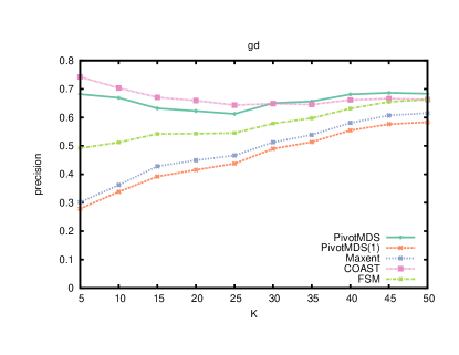
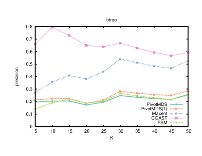
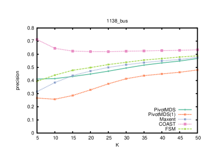
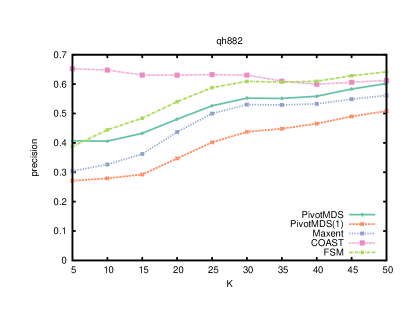
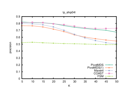
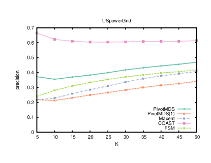
Following Gansner et al. [11], we look at the precision of neighborhood preservation. We are interested in answering the question: if we see vertices nearby in the embedding, how many of these are actually also neighbors in the graph space? We define the precision of neighborhood preservation as follows. For each vertex $i$, $K$ neighboring vertices of $i$ in the layout are chosen. These $K$ vertices are then checked to see if their graph distance is less than a threshold $d(K)$, where $d(K)$ is the distance of the $K$-th closest vertex to $i$ in the graph space. The percentage of the $K$ vertices that are within the threshold, averaged over all vertices $i$, is taken as the precision. Note that precision (the fraction of retrieved instances that are relevant) is a well-known concept in information retrieval. Chen and Buja [3] use a similar concept called LC meta-criteria.

Figure 1: Precision of neighborhood preservation of the algorithms, as a function of $K$. The higher the precision, the better.

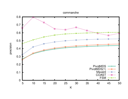Figure 1 gives the precision as a function of $K$ for two representative graphs. From the figure, it is seen that, in general, COAST has the highest, or nearly the highest, precision. PivotMDS(1) tends to have low precision. The precision of other algorithms, including Maxent, tends to be between these two extremes.

Overall, precision of neighborhood preservation is a way to look at one aspect of embedding not well-captured by the full stress objective function, but is important to applications such as recommendations. COAST performs well in this respect.

5 Conclusion and Future Work

In this paper, we described a new technique for graph layout that attempts to satisfy edge length constraints. This technique uses a modified two-part stress function, one part for the edge lengths, the other to guide the relative placement of other node pairs. The stress is quartic in the positions of the nodes, and can be transformed to a form that is suitable for solution using convex programming. The results produced are good and the algorithm is scalable to large graphs.

Although the performance of the COAST algorithm is already competitive, we rely on an ad hoc implementation using a combination of Python, Matlab and C code. It would be very desirable to re-implement the algorithm entirely in C.

Our technique follows the general strategy of doing length-sensitive drawings for large graphs by reformulating the energy function, keeping the core length constraints, and then applying some appropriate mathematical machinery. Variations of this technique have been successfully used by others [16, 11]. It would be interesting to explore additional adaptations of this approach.

References

- [1] Brandes, U., Pich, C.: Eigensolver methods for progressive multidimensional scaling of large data. In: Kaufmann, M., Wagner, D. (eds.) Proc. 14th Intl. Symp. Graph Drawing. LNCS, vol. 4372, pp. 42–53. Springer, Berlin (2007)
- [2] Brandes, U., Pich, C.: An experimental study on distance based graph drawing. In: Tollis, I., Patrignani, M. (eds.) Proc. 16th Intl. Symp. Graph Drawing. LNCS, vol. 5417, pp. 218–229. Springer, Berlin (2009)
- [3] Chen, L., Buja, A.: Local multidimensional scaling for nonlinear dimension reduction, graph drawing, and proximity analysis. J. Amer. Statistical Assoc. 104, 209–219 (2009)
- [4] Chung, F.R.K.: Spectral Graph Theory (CBMS Regional Conference Series in Mathematics, No. 92). American Mathematical Society, Providene, RI (1996)
- [5] Davis, T.A., Hu, Y.: U. of Florida Sparse Matrix Collection. ACM Transaction on Mathematical Software 38, 1–18 (2011), http://www.cise.ufl.edu/research/sparse/matrices/
- [6] Drineas, P., Frieze, A.M., Kannan, R., Vempala, S., Vinay, V.: Clustering large graphs via the singular value decomposition. Machine Learning 56, 9–33 (2004)
- [7] Eades, P.: A heuristic for graph drawing. Congressus Numerantium 42, 149–160 (1984)
- [8] Fruchterman, T.M.J., Reingold, E.M.: Graph drawing by force directed placement. Software - Practice and Experience 21, 1129–1164 (1991)
- [9] Gajer, P., Goodrich, M.T., Kobourov, S.G.: A fast multi-dimensional algorithm for drawing large graphs. In: Marks, J. (ed.) Proc. 8th Intl. Symp. Graph Drawing. vol. 1984, pp. 211 – 221. Springer, Berlin (2000)
- [10] Gansner, E.R., Koren, Y., North, S.C.: Graph drawing by stress majorization. In: Pach, J. (ed.) Proc. 12th Intl. Symp. Graph Drawing. LNCS, vol. 3383, pp. 239–250. Springer, Berlin (2004)
- [11] Gansner, E.R., Hu, Y., North, S.C.: A maxent-stress model for graph layout. IEEE Trans. Vis. Comput. Graph. 19(6), 927–940 (2013)
- [12] Hachul, S., Jünger, M.: Drawing large graphs with a potential field based multilevel algorithm. In: Pach, J. (ed.) Proc. 12th Intl. Symp. Graph Drawing. LNCS, vol. 3383, pp. 285–295. Springer, Berlin (2004)
- [13] Hu, Y.: Efficient and high quality force-directed graph drawing. Mathematica Journal 10, 37–71 (2005)
- [14] Johnson, D.B.: Efficient algorithms for shortest paths in sparse networks. J. ACM 24(1), 1–13 (Jan 1977)
- [15] Kamada, T., Kawai, S.: An algorithm for drawing general undirected graphs. Information Processing Letters 31, 7–15 (1989)
- [16] Khoury, M., Hu, Y., Krishnan, S., Scheidegger, C.: Drawing large graphs by low-rank stress majorization. Computer Graphics Forum 31(3), 975–984 (2012)
- [17] Koren, Y., Çivril, A.: The binary stress model for graph drawing. In: Tollis, I., Patrignani, M. (eds.) Proc. 16th Intl. Symp. Graph Drawing. LNCS, vol. 5417, pp. 193–205. Springer, Berlin (2008)
- [18] Kruskal, J.B.: Multidimensioal scaling by optimizing goodness of fit to a nonmetric hypothesis. Psychometrika 29, 1–27 (1964)
- [19] Kruskal, J.B., Seery, J.B.: Designing network diagrams. In: Proc. First General Conference on Social Graphics. pp. 22–50. U. S. Department of the Census, Washington, D.C. (Jul 1980), Bell Laboratories Technical Report No. 49
- [20] Noack, A.: Energy models for graph clustering. J. Graph Algorithms and Applications 11(2), 453–480 (2007)
- [21] Noack, A.: Modularity clustering is force-directed layout. Physical Review E 79:026102 (2009)
- [22] Pettie, S.: A new approach to all-pairs shortest paths on real-weighted graphs. Theoretical Computer Science 312(1), 47–74 (Jan 2004)
- [23] de Silva, V., Tenenbaum, J.B.: Global versus local methods in nonlinear dimensionality reduction. In: Advances in Neural Information Processing Systems 15. pp. 721–728. MIT Press, Cambridge, MA (2003)
- [24] Tütüncü, R.H., Toh, K.C., Todd, M.J.: Solving semidefinite-quadratic-linear programs using SDPT3. Mathematical Programming 95(2), 189–217 (2003)
- [25] Walshaw, C.: A multilevel algorithm for force-directed graph drawing. J. Graph Algorithms and Applications 7, 253–285 (2003)