Multi-Wavelength Observations of the Spatio-Temporal Evolution of Solar Flares with AIA/SDO: II. Hydrodynamic Scaling Laws and Thermal Energies

Abstract

In this study we measure physical parameters of the same set of 155 M and X-class solar flares observed with AIA/SDO as analyzed in Paper I, by performing a differential emission measure (DEM) analysis to determine the flare peak emission measure $EM_{p}$, peak temperature $T_{p}$, electron density $n_{p}$, and thermal energy $E_{th}$, in addition to the spatial scales $L$, areas $A$, and volumes $V$ measured in Paper I. The parameter ranges for M and X-class flares are: $\log(EM_{p})=47.0-50.5$, $T_{p}=5.0-17.8$ MK, $n_{p}=4\times 10^{9}-9\times 10^{11}$ cm^-3, and thermal energies of $E_{th}=1.6\times 10^{28}-1.1\times 10^{32}$ erg. We find that these parameters obey the Rosner-Tucker-Vaiana (RTV) scaling law $T_{p}^{2}\propto n_{p}L$ and $H\propto T^{7/2}L^{-2}$ during the peak time $t_{p}$ of the flare density $n_{p}$, when energy balance between the heating rate $H$ and the conductive and radiative loss rates is achieved for a short instant, and thus enables the applicability of the RTV scaling law. The application of the RTV scaling law predicts powerlaw distributions for all physical parameters, which we demonstrate with numerical Monte-Carlo simulations as well as with analytical calculations. A consequence of the RTV law is also that we can retrieve the size distribution of heating rates, for which we find $N(H)\propto H^{-1.8}$, which is consistent with the magnetic flux distribution $N(\Phi)\propto\Phi^{-1.85}$ observed by Parnell et al. (2009) and the heating flux scaling law $F_{H}\propto HL\propto B/L$ of Schrijver et al. (2004). The fractal-diffusive self-organized criticality model in conjunction with the RTV scaling law reproduces the observed powerlaw distributions and their slopes for all geometrical and physical parameters and can be used to predict the size distributions for other flare datasets, instruments, and detection algorithms.

1 INTRODUCTION

Nonlinear energy dissipation processes governed by self-organized criticality (SOC) exhibit the ubiquitous powerlaw distribution functions. One of the most intriguing questions in this context is still: Why does nature produce powerlaws? And the very next question is: Can we understand or predict the value of the powerlaw slopes? While Per Bak attempted to explain the powerlaw nature of size distributions of SOC avalanches with the functional form of power spectra, such as the 1/f-noise characteristics that naturally occurs in many systems (Bak et al. 1987), we proposed an even more fundamental explanation for the existence of powerlaws, namely the mere statistical probability of avalanche sizes that can occur in a SOC system with scale-free properties, which scales with $N(L)\propto L^{-d}$, where $d$ is the Euclidean dimension of the SOC system (Aschwanden 2012a,b; 2013a,b). This fundamental relationship, which we call the scale-free probability conjecture, predicts directly the size distributions for avalanche areas $N(A)\propto A^{-2}$ and volumes $N(V)\propto V^{-5/3}$. This prediction follows from the elementary geometrical relationships that the area scales with the square of the length scale, $A\propto L^{2}$, and the volume scales with the third power of the length scale, $V\propto L^{3}$. While the geometric parameters $L$, $A$, and $V$ are space-filling within the Euclidean dimension $d$, the internal structure of avalanches is highly inhomogeneous and can be characterized with a fractal dimension $D_{d}\leq d$, so that the instantaneous avalanche area and volume obey the scaling laws $A\propto L^{D_{2}}$ and $V\propto L^{D_{3}}$, where $D_{2}$ and $D_{3}$ are the Haussdorf dimensions in 2D and 3D space (Aschwanden 2012a). These elementary geometric relationships are probably the simplest scaling laws known in nature. A convenient property of multiplicative or power-exponent scaling laws is that the powerlaw function of a size distribution of one parameter transforms into another, which is the ultimate reason why we find so many powerlaw distributions in nature.

If we want to understand the powerlaw-like size distributions found for many observables and physical parameters in solar flares, as well as to understand the mutual relationships between the powerlaw slopes of these parameters, we have obviously to look into scaling laws, which is the subject of this study. In Paper I (Aschwanden, Zhang, and Liu 2013a) we investigated the spatial and temporal scales of solar flares and found them to be consistent with the scale-free probability conjecture $N(L)\propto L^{-3}$ for the 3D Euclidean space, and with a random walk transport process $L\propto\tau^{\beta/2}$ with sub-diffusive characteristics ($\beta<1$). Analyzing EUV and soft X-ray observations of solar flares involves the physical parameters of heated plasma that radiates during a flare, which can be described by the macroscopic parameters of electron temperatures $T_{e}$, electron densities $n_{e}$, ideal gas pressures $p=2n_{e}k_{B}T_{e}$, emission measures $EM$, and thermal energies $E_{th}$. Statistics of such flare parameters has been gathered for limited samples in the past, such as for flares observed in soft X-rays and EUV (Pallavicini et al. 1977; Shimizu 1995; Feldman et al. 1995a,b, 1996; Porter and Klimchuk 1995; Kano and Tsuneta 1995, 1996; Metcalf and Fisher 1996; Sterling et al. 1997; Kankelborg et al. 1997; Reale et al. 1997; Garcia 1998), or for nanoflares observed in EUV (Berghmans et al. 1998; Krucker and Benz 2000; Parnell and Jupp 2000; Aschwanden et al. 2000; Aschwanden and Parnell 2002). A universal scaling law involving a hydrostatic and a magnetic relationship was proposed by Shibata and Yokoyama (1999). Empirical two-parameter scaling relationships were explored by Aschwanden (1999). Most of these studies were motivated by testing the loop heating scaling law of Rosner-Tucker-Vaiana (RTV) (Rosner et al. 1978) or by testing whether the energy distribution of nanoflares is identical with that of larger flares. Several of these studies suffered from insufficient broadband temperature coverage, which leads to significant underestimates of the flare energy and even affects the powerlaw slope of their distributions (e.g., Benz and Krucker 2002; Aschwanden and Parnell 2002), revealing incompatible results and triggering disputes about the true flare energy distribution. A unified flare energy distribution was attempted by synthesizing statistics from different observers, instruments, and detection algorithms on the same scale (e.g., Fig. 10 in Aschwanden et al. 2000), but doubts remained about the compatibility of different analysis methods and the role of different activity levels of the solar cycle. No study has been tackled yet that provides a consistent statistics of solar flares from the largest to the smallest flare events. The obvious next step in establishing reliable size distributions of flare energies therefore calls for a single instrument that has broadband temperature coverage and sufficient cadence to sample the peak time of the maximum energy release in flares with adequate time resolution. The answer to this call is the AIA/SDO instrument, which allows us to measure all spatial, temporal, and physical parameters with unprecedented quality. In this Paper II we perform a differential emission measure (DEM) analysis of the same 155 large flare events (M and X GOES class) for which we analyzed the spatio-temporal parameters in Paper I. Future studies will continue to smaller classes of flares, and ultimately reveal the true size distribution of flares from the largest events down to the nanoflare regime.

The content of this paper includes a description of the observations, the data analysis, and the results in Section 2, theoretical modeling of the size distributions and correlations in terms of the RTV scaling law in Section 3, a discussion of the results in a larger context in Section 4, and conclusions in Section 5.

2 OBSERVATIONS, DATA ANALYSIS, AND RESULTS

2.1 AIA Observations

The dataset we are analyzing here is identical with that of Paper I (Aschwanden, Zhang, and Liu 2013a) and an earlier single-wavelength study on the spatio-temporal flare evolution (Aschwanden 2012b). This dataset consists of 155 solar flares that includes all M- and X-class flares detected with the Atmospheric Imaging Assembly (AIA) onboard the Solar Dynamics Observatory (SDO) during the first two years of the mission (from 2010 May 13 to 2012 March 31). All AIA images have a cadence of $\Delta t=12$ s and a pixel size of $\Delta x=0.6\hbox{${}^{\prime\prime}$}\approx 435$ km, which corresponds to a spatial resolution of $2.5\Delta x=1.5\hbox{${}^{\prime\prime}$}\approx 1100$ km. We analyzed about 100 time frames for each flare in seven coronal wavelength filters (94, 131, 171, 193, 211, 304, 335 Å) of AIA/SDO (Lemen et al. 2012; Boerner et al. 2012), which amounts to a total number of $\approx 10^{5}$ images or $\approx 2$ Terabytes of AIA data.

In Paper I we measured the following parameters for each flare: The (time-integrated) flare area $A$ at the peak time $t_{p}$ of the GOES soft X-ray flux (which approximately corresponds to the density peak time and to the end time of nonthermal hard X-rays according to the Neupert effect); the length scale $L=\sqrt{A/\pi}$ defined by the radius of an equivalent circular flare area $A$; the flare volume $V=(3\pi/2)L^{3}$ (defined by a hemisphere with radius $L$), the area fractal dimension $D_{2}=\log{(a)}/\log{(L)}$ (defined by the instantaneous fractal flare area $a$ at time $t_{p}$), the flare duration $\tau$ (defined by the soft X-ray rise time $\tau=t_{p}-t_{start}$, which roughly corresponds to the duration of nonthermal hard X-ray emission according to the Neupert effect), the diffusion coefficient $\kappa$ and the diffusion or spreading exponent $\beta$ (defined by the generalized diffusion equation $L=\kappa\tau^{\beta/2}$), and the maximum expansion velocity $v_{max}$, all measured for each of the seven wavelengths. In this study we measure in addition the peak emission measure $EM_{p}$ and the peak temperature $T_{p}$, which characterize the peak of the differential emission measure (DEM) distribution function at the peak time $t_{p}$ of soft X-ray emission, obtained from the six coronal AIA wavelength fluxes $F_{\lambda}$ at the flare peak time $t_{p}$ (without the 304 Åchannel).

2.2 AIA Temperature Response Functions

AIA has six wavelength filters that are sensitive to highly ionized iron lines at coronal temperatures (94, 131, 171, 193, 211, 335 Å) and one (304 Å) that is sensitive to chromospheric temperatures. The contribution of spectral lines and continuum emission to the EUV channels of AIA/SDO are listed in O’Dwyer et al. (2010), and MHD simulations are provided in Martinez-Sykora et al. (2011). The response functions $R(T)$ of these seven filters are shown elsewhere (e.g., Fig. 13 in Lemen et al. 2012) and can be obtained with the Solar SoftWare (SSW) procedure AIA$\_$GET$\_$RESPONSE. The temperatures range extends to as low as $T\approx 0.1$ MK for the 304 Å filter, and covers the range of $T_{e}\approx 1-20$ MK for the coronal filters (131, 171, 193, 211, 335, and 94 Å). Most filters have a dual response to two temperature ranges, which makes the inversion of the differential emission measure (DEM) distribution more ambiguous. The AIA instrument is described in Lemen et al. (2012) and the calibration is detailed in Boerner et al. (2012). A major update in the AIA instrumental response functions since launch occurred on February 13, 2012, which includes updated emissivities according to the CHIANTI (Version 7) model, and an empirical correction of the 94 and 131 Å sensitivities in the lower temperature range ($log(T)\lower 1.72218pt\hbox{$\;\buildrel<\over{\scriptstyle\sim}\;$}6.3$) due to missing Fe XVIII, XI, and X lines in the CHIANTI model, as reported earlier (Aschwanden and Boerner 2011; Fig. 10 therein). In the present study we used the updated standard response functions that are available in the Interactive Data Language (IDL) based Solar Software (SSW) (status of December 2012).

2.3 Differential Emission Measure Analysis

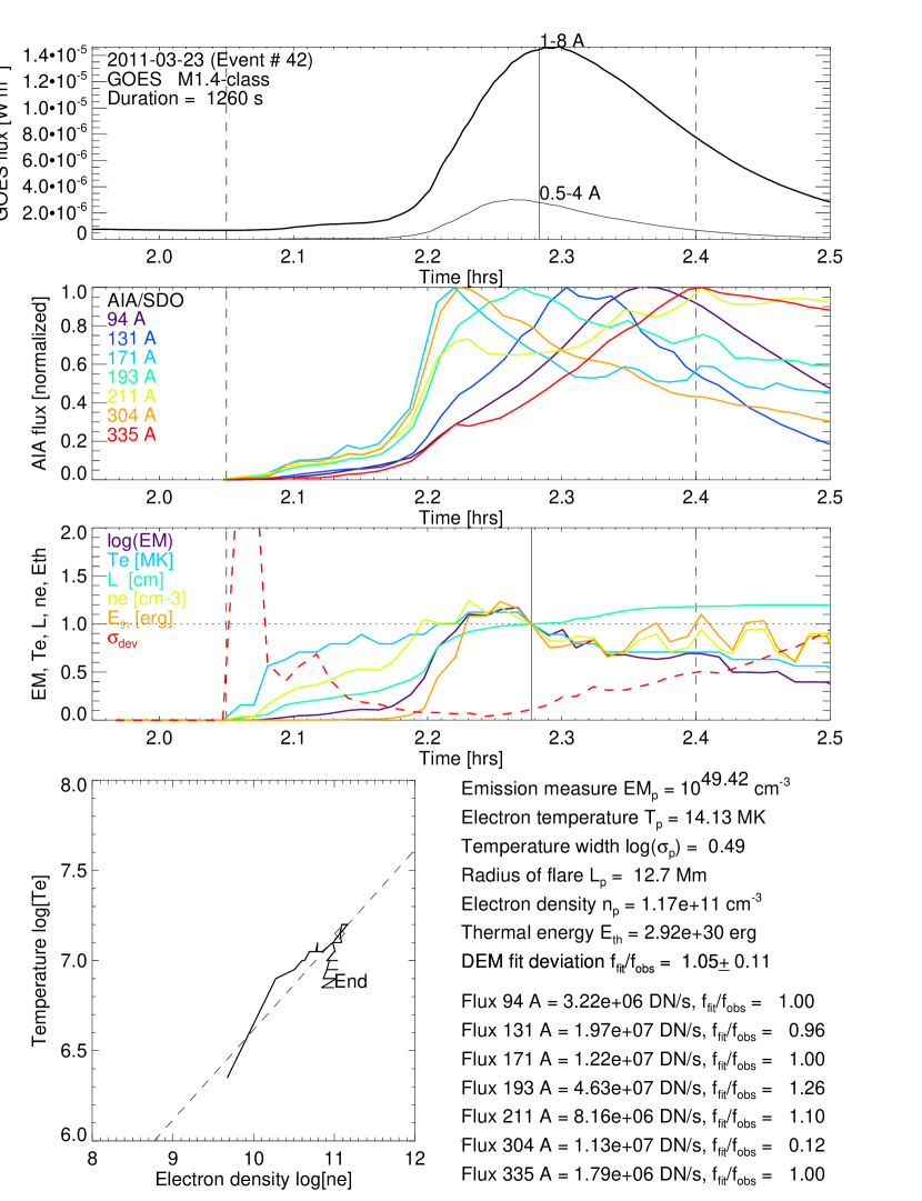
Figure 1: Top panel: GOES time profiles, with time in hrs [UT]; Second panel: AIA time profiles; Third panel: Time profiles of peak emission measure $EM_{p}(t)$, peak temperature $T_{e}(t)$, length scale $L(t)$, electron density $n_{e}(t)$, thermal energy $E_{th}(t)$, and DEM fit quality $\sigma_{dev}$; Fourth panel: Evolutionary phase diagram $T_{p}(n_{e})$. Bottom right: Physical parameters at the flare peak time $t_{p}$, observed total fluxes $f_{obs}$, and DEM fit ratios $f_{fit}/f_{obs}$, fitted at the time of the GOES 1-8 Å peak, here at 2011-03-12, 02:17 UT.

We determine the differential emission measure (DEM) distribution function for each of the $\approx 100$ time intervals (per flare) for the 155 selected M- and X-class flares, in order to obtain the wavelength-independent peak emission measure $EM_{p}$ and DEM peak temperature $T_{p}$ per event. An example of a dataset for one event (observed on 2011 March 23, 2:00-2:30 UT, a GOES M1.4 class flare) is shown in Fig. 1. The GOES time profiles for the soft (1-8 Å) and hard (0.5-4 Å) channels are shown in the top panel of Fig. 1, with the GOES start and end times (vertical dashed lines in Fig. 1) and flare peak time $t_{p}$ (vertical solid line in Fig. 1) indicated. The accompanying AIA/SDO time profiles for all seven filters are shown in the second panel of Fig. 1. From the colored time profiles one can identify that the 171, 211, and 193 Å channels peak before the GOES soft channel, while the 131, 94, 335, and 304 channels peak after the GOES channel. Thus, the EUV channels peak over a range of time (02:12-02:24 UT). With the DEM analysis we deduce the time evolution of the total emission measure $EM(t)$ (integrated over the flare area) and electron temperature $T_{e}(t)$.

Our observational constraints are the six EUV fluxes $F_{\lambda}(t)$, since we ignore the chromospheric channel $\lambda=304$ Å in DEM fits. In the following, the flux $F_{\lambda}$ (DN s^-1) always refers to the total flux integrated over the flare area, and the total emission measure $EM$ (cm^-3) is integrated over the entire flare volume. We subtract a preflare-background flux $F_{\lambda}(t_{b})$ in each channel, which is believed to originate from flare-unrelated emission in the active region, determined from the minimum flux in the time interval $t_{start}<t_{b}<t_{peak}$ between the GOES flare start time $t_{start}$ and the GOES flare peak time $t_{p}$. These background-subtracted loop fluxes in each of the six coronal wavelength filters can be related to the DEM distribution function $dEM(T)/dT$ of the flare at time $t$ by

$$F_{\lambda}(t)-F_{\lambda}(t_{b})=\int{dEM(T,t)\over dT}R_{\lambda}(T)\ dT=\sum_{k}EM(T_{k},t)R_{\lambda}(T_{k})\Delta T_{k}\ ,$$ (1)

where $R_{\lambda}(T)$ is the instrumental temperature response function of each filter $\lambda$. The particular functional shape of the DEM function $dEM(T,t)/dT$ is unknown and can be quite complex, based on DEM reconstructions of solar flare multi-wavelength observations (e.g., Battaglia and Kontar 2012; Graham et al. 2013). Also, the DEM reconstruction from AIA data is not necessarily reliable, based on simulations with known DEMs from MHD simulations, although acceptable $\chi^{2}$-values may be obtained (e.g., Testa et al. 2012). Nevertheless, for sake of simplicity, the temperature peak of a DEM distribution can be characterized with a minimum of three free parameters, such as with a Gaussian function in the logarithm of the temperature,

$$EM(T,t_{i})=EM_{i}\exp{\left(-{[\log(T)-\log(T_{i})]^{2}\over 2\sigma_{i}^{2}}\right)}\ ,$$ (2)

which has three free parameters for every time $t_{i}$. At the density peak time $t_{i}=t_{p}$ of the flare, this defines the peak emission measure $EM_{p}$, the DEM peak temperature $T_{p}$, and the Gaussian temperature width $\sigma_{p}$. The observed functions $F_{\lambda}(t)$ can then be fitted simply by calculating the convolution of the DEM function $dEM(T)/dT$ with the filter response functions $R_{\lambda}(T)$ (Eq. 1) for a set of discretized temperatures $T_{i},i=0,...,n_{T}$ and Gaussian widths $\sigma_{j},j=1,...,n_{\sigma}$, while the emission measure $EM_{p}$ is just a constant that can be obtained from the ratio of the left-hand and right-hand side terms of Eq. 1, using the median value among the six wavelengths. The choice of a Gaussian is one of the simplest functions to model a DEM, and thus most robust, but we caution that it may not be adadequate to characterize some broadband DEMs.

The best fit of the parameters $T_{p}$ and $\sigma_{p}$ is normally obtained by a chi-square fit, which requires knowledge of the expectation value of the uncertainty $\sigma_{F}$ in the count rate $F$ in each filter. For the Poisson statistics of the photons, which is for AIA approximately equal to the the counts $C=F\times t_{exp}$ recorded during the exposure time $t_{exp}$, the expectation value of the uncertainty is $\sigma_{C}=\sqrt{C}$ (e.g., see Aschwanden and Boerner 2011 for a DEM analysis of coronal loops using AIA data). In the case of total emission measure modeling of flares as applied here, photon statistics can be neglected, because the largest uncertainty comes from the inadequacy of the chosen functional form of the DEM, and from the estimation of the subtracted preflare background, which is difficult (or impossible) to quanitfy a priori, since the background has large spatial and temporal variations that cannot easily be separated from flare-related EUV emission. However, we can straightforwardly quantify a measure of the goodness-of-fit by the ratios of the fitted to the observed fluxes, in terms of a mean and r.m.s. standard deviation $\sigma_{dev}$,

$$\sigma_{dev}=\left[{1\over n_{\lambda}}\sum_{\lambda}(f_{fit,\lambda}-f_{obs,\lambda})^{2}\right]^{1/2}\ .$$ (3)

Minimizing this fitting criterion in each DEM fit (for each time $t$) we obtain the time evolution of the peak emission measure $EM_{p}(t)$, peak temperature $T_{p}(t)$, and Gaussian temperature width $\sigma_{p}(t)$. We found a most robust optimization by using the goodness-of-fit measure $\sigma_{dev}$ as a weighting factor $w_{ij}=1/\sigma_{dev,ij}^{2}$ in averaging all trial values of $T_{i}$ and $\sigma_{j}$,

$$T_{p}={\Sigma_{i}^{n_{T}}\Sigma_{j}^{n_{\sigma}}T_{i}w_{ij}\over\Sigma_{i}^{n_{T}}\Sigma_{j}^{n_{\sigma}}w_{ij}}\ ,$$ (4)

$$\sigma_{p}={\Sigma_{i}^{n_{T}}\Sigma_{j}^{n_{\sigma}}\sigma_{j}w_{ij}\over\Sigma_{i}^{n_{T}}\Sigma_{j}^{n_{\sigma}}w_{ij}}\ .$$ (5)

The time evolution of the emission measure $EM_{p}(t)$ and electron temperature $T_{p}(t)$ at the peak of the DEM are shown in the third panel of Fig. 1. The logarithmic (Gaussian) temperature width $\sigma_{p}$ of the DEM at the peak time is found to have a mean and standard deviation of $\sigma_{p}=0.50\pm 0.13$ (for the entire set of 155 flares), but is not correlated with either the temperature $T_{p}$ or emission measure $EM_{p}$. So, the average full width at half maximum (FWHM) of the flare DEMs is $log({\rm FWHM}_{T})\approx 2.35\sigma_{p}\approx 1.18$. This is quite a broad DEM function. For instance, for a typical flare peak temperature of $T_{p}\approx 10$ MK we have a FWHM temperature range from $T_{1}=T_{p}-{\rm FWHM}_{T}/2=2.5$ MK to $T_{2}=T_{p}+{\rm FWHM}_{T}/2=40$ MK.

Using furthermore the spatial length scale $L(t)$ and volume $V(t)$ as determined in Paper I, we can then also derive the time evolution of the average electron density (averaged over the flare volume),

$$n_{e}(t)=\sqrt{EM_{p}(t)\over V(t)}\ ,$$ (6)

where the flare volume $V(t)$ is approximated by a hemispheric geometry, $V(t)=(2/3)\pi L(t)^{3}$. In addition we infer also the time evolution of the thermal energy,

$$E_{th}(t)=3\ n_{e}(t)k_{B}T_{p}(t)V(t)\ .$$ (7)

These time evolutions are also shown in the third panel of Fig. 1, where it can be clearly discerned that all quantities, i.e., the emission measure, the temperature, the density, and the thermal energy monotonically increase before the flare peak, while all drop after the flare peak, except for the flare size $L(t)$ and volume $V(t)$. The fitting quality of this example is quite satisfactory, as it can be seen from the ratio of the fitted to the observed fluxes, with a mean and standard deviation of $f_{fit}/f_{obs}=1.05\pm 0.11$ (listed in Fig. 1, bottom right). In other words, the DEM at the flare peak time can be characterized by a Gaussian function that reproduces all 6 coronal EUV fluxes with an accuracy of $\approx 15\%$ (except for the 304 Å channel, which is of chromospheric origin and ignored here). An evolutionary temperature-density phase diagram $T_{p}(n_{p})$ is shown in the lower left panel in Fig. 1, revealing a density and temperature increase that closely follows the RTV law (dashed diagonal line) during the flare rise time, while it deviates from the RTV equilibrium during the beginning of the cooling phase as expected from hydrodynamic simulations (e.g., Jakimiec et al. 1992; Sterling et al. 1997; Aschwanden and Tsiklauri 2009).

In the remainder of the paper we will ignore the time evolution and deal with statistics of the physical parameters measured at the GOES peak time $t_{p}$ only, which approximately equals the peak time of the flare emission measure $EM_{p}$ or density $n_{p}$. We label the parameters briefly as $T_{p}=T_{e}(t=t_{p})$ (not to be confused with the temperature maximum time $t_{m}$ that occurs earlier than the density peak time $t_{p}$), $EM_{p}=EM(t=t_{p},T_{e}=T_{p})$, $n_{p}=n_{e}(t=t_{p},T_{e}=T_{p})$, and $E_{th}=E_{th}(t=t_{p},T_{e}=T_{p})$. In the example shown in Fig. 1, these values amount to $EM_{p}=10^{49.42}$ cm^-3, $T_{p}=14.13$ MK, $log(\sigma_{T})=0.49$, $L_{p}=12.7$ Mm, $n_{p}=1.17\times 10^{11}$ cm^-3, and $E_{th}=2.92\times 10^{30}$ erg.

The best-fit parameters of the DEM analysis ($T_{p},\sigma_{p},EM_{p},E_{th}$, and $F_{fit}/F_{obs}$) are tabulated in Table 2 for all 155 analyzed events. Note that the length scale $L_{p}$ listed in Table 2 refers to the radius of the time-integrated flare area above some flux threshold, which may deviate somewhat from the values $L$ measured from the radial expansion with preflare-area subtraction in Aschwanden (2012b). We identify a few events that represent outliers regarding the peak temperature $T_{p}\lower 1.72218pt\hbox{$\;\buildrel<\over{\scriptstyle\sim}\;$}5$ MK (events #11, 18, 90, 100), emission measure $\log(EM_{p})\lower 1.72218pt\hbox{$\;\buildrel<\over{\scriptstyle\sim}\;$}47.5$ (events #7, 26, 90, 139), or DEM fit quality ($F_{fit}/F_{obs}\lower 1.72218pt\hbox{$\;\buildrel>\over{\scriptstyle\sim}\;$}1$) (event #90), which partially are affected by preflare background problems or other data irregularities.

2.4 Observed Size Distributions

The size distributions of the physical parameters of the 155 analyzed flares are shown in Fig. 2, which are all wavelength-independent, because the DEM analysis synthesizes the contributions from all different wavelengths into an instrument-independent DEM distribution function. Besideds the powerlaw part on the right side of the distribution, there is also a rollover at the left side due to incomplete sampling.

The geometric parameters show powerlaw distributions with the universal values for their slopes, i.e., $\alpha_{L}=2.80\pm 0.16$ (Fig. 2a, predicted as $\alpha_{L}=3.00$ from the FD-SOC model) for length scales within a range of $L=4-64$ Mm, in agreement with the averaged values from all wavelengths and flux thresholds in Paper I, namely $\alpha_{L}=3.20\pm 0.71$. The powerlaw slope of the flare volumes is found to be $\alpha_{V}=1.62\pm 0.04$ (Fig. 2b, predicted as $\alpha_{V}=5/3\approx 1.67$ from the FD-SOC model) for volumes in a range of $V=2\times 10^{26}-5\times 10^{29}$ cm^-3.

For the physical parameters we find from the DEM analysis the following ranges and powerlaw slopes: emission measure $EM_{p}=10^{47.0}-10^{50.5}$ cm^-3, $\alpha_{EM}=1.78\pm 0.03$ (Fig. 2c); electron temperature $T_{P}\approx 5.0-17.8$ MK (Fig. 2d); electron density $n_{P}\approx 4\times 10^{9}-9\times 10^{11}$ cm^-3, $\alpha_{n}=2.15\pm 0.17$ (Fig. 2e); and thermal energy $E_{th}=1.6\times 10^{28}-1.1\times 10^{32}$ erg, $\alpha_{Eth}=1.66\pm 0.13$ (Fig. 2f). We note that the powerlaw slopes of the flare volume ($\alpha_{V}=1.62\pm 0.04$. Fig. 2b), peak emission measure ($\alpha_{EM}=1.78\pm 0.03$, Fig. 2c), and thermal energy ($\alpha_{Eth}=1.66\pm 0.13$, Fig. 2f) are almost identical, and thus these three parameters are almost proportional to each other. By defining a powerlaw scaling between two parameters $x$ and $y$, i.e., $x\propto y^{\gamma}$ with $N(x)\propto x^{-\alpha_{x}}$, $N(y)\propto y^{-\alpha_{y}}$, and $\gamma=(\alpha_{x}-1)/(\alpha_{y}-1)$, we find the following powerlaw relationships between the three parameters $V_{p}$, $EM_{p}$, and $E_{th}$,

$$EM_{p}\propto V^{\gamma_{EM}}\ ,\qquad\gamma_{EM}={\alpha_{V}-1\over\alpha_{EM}-1}=0.80\pm 0.07\ ,$$ (8)

$$E_{th}\propto V^{\gamma_{Eth}}\ ,\qquad\gamma_{Eth}={\alpha_{V}-1\over\alpha_{Eth}-1}=0.85\pm 0.07\ ,$$ (9)

$$E_{th}\propto EM_{p}^{\gamma_{E}}\ ,\qquad\gamma_{E}={\alpha_{EM}-1\over\alpha_{Eth}-1}=1.23\pm 0.29\ .$$ (10)

These relationships allow us to predict the thermal flare energy $E_{th}$ from the observed peak emission measure $EM_{p}$ directly, without need of spatial observations, which may be used in the case of stellar observations. Alternatively, we can predict the geometric volume $V_{p}$ (or the spatial size of the flare) from the observed emission measure $EM_{p}$, which may be used for both solar and stellar non-imaging observations, supposed that flares on the Sun and on stars obey the same scaling law.

The size distributions of peak temperatures and densities, $N(T_{p})$ and $N(n_{p})$, cannot straightforwardly be predicted from two-parameter correlations, since we expect three-parameter relationships $(T_{p},n_{p},L_{p})$ for RTV-type scaling laws (see Section 3).

The size distributions of peak fluxes $F_{\lambda}$ for the AIA channels with wavelengths $\lambda=$ 94, 131, 171, 193, 211, 304, and 335 Å have an approximate powerlaw slope of $\alpha_{F}\approx 2.0$ (Table 1). A breakdown of the fitted powerlaw slopes $\alpha_{\lambda}$ by wavelengths $\lambda$ and flux thresholds for flare area detection $q_{thresh}=$ 0.01, 0.02, 0.05, 0.1, and 0.2 is listed in Table 1, which yield a mean and standard deviation of $\alpha_{\lambda}=2.06\pm 0.13$. The lack of any significant wavelength dependence implies a very good correlation between fluxes in different wavelengths, which is expected for broadband DEM functions and/or broadband instrumental response functions.

2.5 Observed Flux-Flux Correlations

Optically-thin emission in soft X-ray and EUV lines are expected to correlate with the flare volume, since the observed fluxes $F_{\lambda}$ scale with the emission measure $EM$ (Eq. 1), and thus with the total flare volume $V$, since $EM=\int n_{e}^{2}dV$ (Eq. 6). We show the flux-volume correlations in form of scatterplots and linear regression fits in Fig. 3 (top and second row). The linear regression fits use the orthogonal reduced major axis method (Isobe et al. 1990). The Pearson cross-correlation coefficient of the AIA flare peak fluxes $F_{p}$ with the inferred flare volumes $V_{p}$ (Paper I) vary from the lowest value $ccc=0.18$ for the 193 Å wavelength to $ccc=0.70$ for the 335 Å wavelength. The relatively low values for the 171 and 193 Å channels probably result from the effects of EUV dimming, which cause an underestimate of cool ($T_{e}=1-2$ MK) plasma due to coronal mass ejections (Aschwanden et al. 2013a; Paper I, Section 4.4). Interestingly, the linear regression coefficient $\gamma$ obtained from the correlation $F_{AIA}\propto V^{\gamma}$ behaves similar to the cross-correlation coefficient, namely the slope is highest and nearest to proportionality for 335 Å ($\gamma_{335}=0.59\pm 0.05$ and $ccc=0.70$), while it is lowest for 193 Å($\gamma_{193}=0.16\pm 0.08$ and $ccc=0.16$). Thus, both the cross-correlation coefficient $ccc$ and the linear regression slope $\gamma_{\lambda}$ are a measure of the flux-volume proportionality. We will discuss the wavelength-dependent flux-volume relationships in Section 3.5.

The GOES flux (of the soft 1-4 Å channel) is often used to define the flare magnitude (such as in the selection of M- and X-class flares used here). We show the correlations between the EUV peak fluxes $F_{AIA,\lambda}$ and the GOES peak fluxes $F_{GOES}$ measured at the flare peak time $t_{p}$, both preflare-background subtracted, in Fig. 3 (third and bottom row). We see that the best correlations with the GOES soft X-ray flux occur for those EUV channels that are sensitive to high temperatures, such as 193 Å (ccc=0.82), 131 Å (ccc=0.79), and 94 Å(ccc=0.74), while it is lowest for chromospheric temperatures as seen with 304 Å (ccc=0.48). The linear regression fits show correlations between the AIA and GOES fluxes, $F_{AIA,\lambda}\propto F_{GOES}^{\delta_{\lambda}}$, with $\delta_{\lambda}=1.04\pm 0.13$, excluding the 304 Å channel. The three hottest EUV channels (193, 131, 94 Å) thus represent some proxies of the GOES fluxes or flare magnitude, as expected to some degree from the GOES high-temperature response function (White et al. 2004). A recent study used the 193 Å channel on the STEREO spacecraft, which besides the peak sensitivity to $T_{e}\approx 1.5$ MK plasma includes also an Fe XXIV line at 192 Å that enables a secondary sensitivity at 15 MK, to estimate the GOES magnitude of occulted or behind-the-limb flares (Nitta et al. 2013).

3 THEORETICAL MODELING

In this study we determined physical parameters of flares, such as electron temperatures $T_{e}$ and electron densities $n_{e}$, using a multi-wavelength differential emission measure (DEM) analysis that provides the DEM peak emission measure $EM_{p}$ and peak temperature $T_{p}$ at the flare density peak time $t_{p}$. In order to understand the underlying physical scaling laws, their statistical distributions, and correlations, we have to relate these physical parameters to the geometric parameters (length scale $L$, flare area $A$, flare volume $V$, and fractal dimension $D_{d}$) determined in Paper I. Our theoretical model is based on the RTV (Rosner, Tucker, and Vaiana 1978) scaling law (Section 3.1), which provides a useful tool that can be applied at the flare peak time to multi-loop flare geometries (Section 3.2) and can predict parameter correlations and powerlaw distributions of the observed parameters (Section 3.3-3.5).

3.1 The RTV Scaling Law

The RTV scaling law (Rosner et al. 1978) describes a hydrostatic equilibrium solution of a coronal loop that is steadily and spatially uniformly heated, has a constant pressure, and is in equilibrium between the volumetric heating rate and the losses by radiation and thermal conduction, yielding a scaling law between the loop maximum temperature at the apex, the (constant) pressure, and the loop half length, as well as a scaling law for the (constant) volumetric heating rate. Although this scaling law is generally applied to one-dimensional (1-D) coronal loops, the assumption of steady heating and spatial uniformity of the heating function is often questioned, because observations and hydrodynamic modeling suggest impulsive heating functions (e.g., Warren et al. 2003) and non-uniform (footpoint) heating (e.g., Aschwanden et al. 2001).

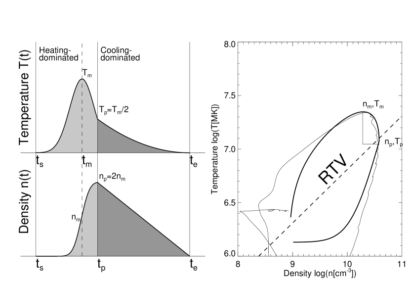
Figure 4: Hydrodynamic time evolution of the electron temperature $T(t)$ and density $n_{e}(t)$ of a simulation of an impulsively-heated flare loop (see Aschwanden and Tsiklauri 2009), shown as time profiles (left panel) and as an evolutionary phase diagram $T_{e}(n_{e})$ (right panel). The evolution of the hydrodynamic simulation is shown as exact numerical solution (curve with thin linestyle in right panel), and as an analytical approximation (curves with thick linestyle in both panels, along with the prediction $T_{e}\propto n_{e}^{1/2}$ of the RTV scaling law for uniform steady heating (dashed line in right panel).

Nevertheless, despite the observed violation of the steady-state assumption, the application of the RTV scaling law is probably most adequate at one particular time of an impulsively-heated coronal loop, when it reaches the density peak $n_{p}=n_{e}(t=t_{p})$. At this particular time the energy balance is approximately fulfilled, where the heating rate just matches the energy losses due to thermal conduction and radiative losses. Before the time $t_{p}$, heating dominates over the losses and the temperature rises, while after this time at $t\geq t_{p}$ the energy losses dominate over heating and the loop temperature drops. We illustrate this hydrodynamic behavior in Fig. 4, where the temperature and density evolution is depicted according to a hydrodynamic simulation with an impulsive heating function (see details in Aschwanden and Tsiklauri 2009). In the evolutionary temperature-density phase diagram (Fig. 4, right panel), a phase diagram that has been pioneered extensively with earlier flare data (e.g., Jakimiec et al. 1992; Sylwester et al. 1990, 1993; Sylwester 1996), we can overlay the RTV equilibrium solution $T_{e}\propto n_{e}^{1/2}$ for the simulated loop with a half length of $L_{loop}=5.5\times 10^{9}$ cm. If the loop would be very slowly heated, near-equilibrium energy balance could be achieved and the temperature and density rise should follow the RTV curve. However, the evolutionary curve of the hydrodynamic simulation shows that the loop temperature is always higher than the RTV equilibrium value during the heating-dominated phase, while it is lower during the cooling-dominated phase (Fig. 4, right panel). The RTV solution predicts the correct loop temperature and density only at one point in time, near the peak density time $t=t_{p}$, where the peak density $n_{e}=n_{p}$ is reached and the temperature dropped to about half of the maximum temperature, $T_{p}\approx T_{m}/2$. Thus the RTV law is a useful predictor for the density $n_{p}$ and temperature $T_{p}$ when the emission of the loop is brightest, since the emission measure $EM_{p}$ scales with the squared density $n_{e}$ and line-of-sight column depth $L_{z}$, i.e., $EM_{p}=n_{p}^{2}L_{z}$.

While the foregoing argument was made for a single loop in an active region, we are using now the same argument of the applicability of the RTV scaling law for the flare peak time $t_{p}$, when the thermal emission of a flare in soft X-ray wavelengths is brightest, such as during the GOES peak time $t_{p}$ of the flare. Comparing the evolutionary phase diagram $T_{e}(n_{e})$ of the total flare emission of an observed flare (Fig. 1, bottom left panel) with the hydrodynamic simulation of an impulsively-heated single loop (Fig. 4, right panel), we see a fairly similar evolution, although the flare may consist of multiple loops.

3.2 Multi-Loop Flare Geometries

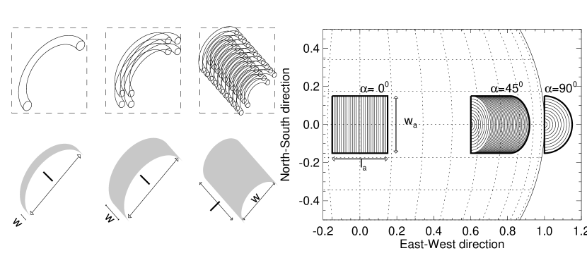
Figure 5: Geometric models of multi-loop flare geometries are pictured in terms of observed length $l$ and width $w$ parameters: single-loop model with width $w\ll l$ (first left panel), small multi-loop model with $w\lower 1.72218pt\hbox{$\;\buildrel<\over{\scriptstyle\sim}\;$}l$ (second left panel), large multi-loop arcade model with $w\leq l$ (third left panel), and a semi-cylindrical flare arcade at various aspect angles from Sun center to limb (right panel).

Can we apply the RTV scaling law to multi-loop geometries? Spatial high-resolution observations from TRACE and AIA/SDO clearly demonstrate the multi-loop structure of solar flares. One particular flare, the Bastille-Day-2000 flare has been modeled in detail and a multitude of at least $\lower 1.72218pt\hbox{$\;\buildrel>\over{\scriptstyle\sim}\;$}100$ individual postflare loops have been identified for this X5.7 GOES-class flare (Aschwanden and Alexander 2001). Even the simplest and smallest nanoflares appear to be composed of multiple loops (e.g., Aschwanden et al. 2000). Such multi-loop geometries can be modeled most simply by arcades of loops, straddling along a neutral line, as visualized in Fig. 5. In Paper I, however, we measured the projected flare area $A(t)$ and defined a length scale

$$L=\sqrt{A/\pi}\ ,$$ (11)

that corresponds to the radius of an equivalent circular area $A$. The question arises now how can we relate this flare length scale $L$ to the loop half length $L_{loop}$ used in the RTV scaling law, and to multi-loop models of flares.

The semi-cylindrical multi-loop arcade model shown in Fig. 5 has a projected area that can be characterized with a rectangular shape with a length $l$ and width $w$, yielding an area of $A=(lw)$, or a radius $L=\sqrt{A/\pi}=\sqrt{lw/\pi}$ of an equivalent circular area $A$. The loop half length $L_{loop}$ for the largest loops contained in the arcade scale as $L_{loop}=(\pi/2)(l/2)$ for single-loop cases, to $L_{loop}=(\pi/2)(w/2)$ for large multi-loop arcades, so the geometric mean is a good approximation,

$$L_{loop}={\pi\over 2}L={\sqrt{\pi lw}\over 2}\ .$$ (12)

In principle, a multi-loop arcade consisting of an array of loops with different (half) lengths $L_{loop}$ as a function of the radial distance $r$ from the neutral line could be modeled by a superposition of RTV loops, according to the scaling laws for the heating rates $H$ and apex temperatures, which can then be summed up to produce a DEM distribution for each time of a flare, and can then be related to the overall length scale $L$ of the flare. However, since the spatial distribution of the heating rate $H$ is unknown and is likely to be spatially non-uniform, no simple model can be made with certainty a priori. Our working assumption is that loops with a half length of $L_{loop}=(\pi/2)L$ demarcate the brightest loops in the flare arcade, from which the flare area $A=\pi L^{2}$ is measured, and thus this loop (half) length $L_{loop}=(\pi/2)L$ is the most relevant parameter in the application of the RTV law to estimate the peak emission measure $EM_{p}$ and peak temperature $T_{p}$ for a flare with a hemispheric volume $V=(2\pi/3)L^{3}$ and radius $L$.

3.3 Observational Test of the RTV Scaling Law

The RTV law (Rosner et al. 1978) specifies a 3-parameter relationship between the flare peak temperature $T_{p}$, the (spatially averaged) peak electron density $n_{p}$, and length scale $L_{p}=L_{loop}/(\pi/2)$, measured at the flare peak time $t_{p}$. Thus, we can express the RTV law as a function of these three parameters $(T_{p},n_{p},L_{p})$, by inserting $L_{loop}=(\pi/2)L_{p}$ (Eq. 12), and defining $n_{p}=n_{apex}$ and $T_{p}=t_{apex}$, to predict each of the three parameters as a function of the other two,

$$T_{p}=c_{1}\ n_{p}^{1/2}\ L_{p}^{1/2}\ ,\qquad c_{1}=1.1\times 10^{-3}\ ,$$ (13)

$$n_{p}=c_{2}\ T_{p}^{2}L_{p}^{-1}\ ,\qquad c_{2}=8.4\times 10^{5},$$ (14)

$$L_{p}=c_{3}\ T_{p}^{2}n_{p}^{-1}\ ,\qquad c_{3}=8.4\times 10^{5}\ .$$ (15)

These are predicted 3-parameter correlations that can be tested with our data. Another useful parameter is the total emission measure $EM_{p}$, defined by the integral over the flare volume $V$,

$$EM_{p}=\int n_{p}^{2}dV=n_{p}^{2}V=n_{p}^{2}({2\pi\over 3}L_{p}^{3})=c_{4}\ T_{p}^{4}L_{p}\ ,\qquad c_{4}=1.48\times 10^{12}.$$ (16)

Furthermore, we will also determine the distribution of thermal energies,

$$E_{th}=3n_{p}k_{B}T_{p}V_{p}=c_{5}\ T_{p}^{3}L_{p}^{2}\ ,\qquad c_{5}=7.3\times 10^{-10},$$ (17)

which can be expressed as a function of the peak temperature $T_{p}$ and length scale $L_{p}$ by substituting the RTV scaling law for the density $n_{p}$ (Eq. 14). In addition we have the RTV heating rate scaling law,

$$H\approx c_{6}\ T_{max}^{7/2}L_{loop}^{-2}=c_{6}\ T_{p}^{7/2}L_{p}^{-2}\ ,\qquad c_{6}=0.95\times 10^{-6}$$ (18)

Our data provide the measurements of the independent parameters $T_{p}$, $n_{p}$, and $L_{p}$, which allows us to test the applicability of the RTV law. In Fig. 6a we show the RTV-predicted flare peak temperature $T_{RTV}=c_{1}\sqrt{n_{p}L_{p}}$ (Eq. 13) as a function of the observed flare peak temperature $T_{p}$ and find a good agreement within a factor of $T_{RTV}/T_{obs}=1.05\pm 0.38$, which means that the RTV law predicts the flare temperature with an accuracy of $\approx 40\%$ in the range of $T_{p}\approx 4-20$ MK.

Similarly we test the predicted peak densities $n_{RTV}$ (Eq. 14) in Fig. 6b and obtain agreement within a factor of two, i.e., $n_{RTV}/n_{obs}=1.3\pm 2.1$. The predicted loop lengths $L_{RTV}$ (Eq. 15) are shown in Fig. 6c and agree by the same factor, $L_{RTV}/L_{obs}=1.3\pm 2.1$. The peak emission measures $EM_{p}$ (Eq. 16) are shown in Fig. 6d and agree within $log(EM_{RTV}/EM_{obs})=0.44\pm 0.50$, which corresponds to a factor of $10^{0.44}\approx 2.7$. The thermal energies $E_{th}$ (Eq. 17) are shown in Fig. 6e and agree within $E_{RTV}/E_{obs}=1.3\pm 2.1$.

We conclude that the RTV law represents a physical model that is adequate to explain the relationship between geometric flare parameters $(L_{p},A_{p},V_{p})$ and the hydrodynamic fluid parameters of the electron temperature $T_{p}$ and density $n_{p}$ at the time of the flare peak. This corroborates our assumption that energy balance between heating and cooling processes is achieved during the flare peak time, even in the case of a dynamic evolution that is different from the steady-state condition under which the RTV law was derived originally.

3.4 Size Distributions Modeled with the RTV Law

In the next step we like to understand the powerlaw slopes of the observed size distributions (Fig. 2) in terms of the RTV scaling law. The histogrammed distribution functions show powerlaws at the right-hand side of the distributions, but reveal also a rollover at the left-hand side, which is primarily a consequence of incomplete sampling of small events, as well as truncation effects that need to be included in modeling of the size distributions. In Fig. 7 we show the same size distributions as in Fig. 2, but juxtapose also scatterplots of the various parameters (x-axis) with the length scale (y-axis), which clearly show how the rollover in the size distributions relate to truncation effects in the scatterplots. There are two truncation effects that we include in modeling the size distributions: (i) a lower limit $H_{0}\approx 0.04$ erg cm^-3 s^-1 of the heating rate distribution $N(H)$ (shown as dotted vertical line in Fig. 7d), and (ii) a lower limit $EM_{0}=10^{49}$ cm^-3 of the emission measure threshold that results from the GOES flux threshold of M1.0 flares (shown as dashed vertical line in Fig. 7e). The truncation boundaries in the two-parameter scatterplots of flare peak temperatures (Fig. 7b), peak densities (Fig. 7c), and thermal energies (Fig. 7f) that result from these two limits $H_{0}$ and $EM_{0}$ are calculated from the RTV law in Appendix A (Eqs. A1-A4) and are indicated in all panels of Fig. 7 as dotted and dashed lines. We see that these truncation boundaries, caclulated analytically from the RTV law, demarcate the observed ranges of datapoints in the scatterplots quite well. Obviously, they also affect the powerlaw slopes of the parameter distributions.

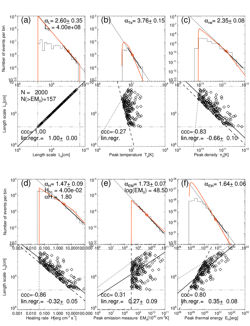
Figure 8: Monte-Carlo simulations of data points (diamonds) using the RTV relationships and a heating rate distribution $N(H)\propto H^{-\alpha_{H}}$ with a minimum value $H_{0}=0.4$ erg cm^-3 s^-1 and powerlaw slope $\alpha_{H}=1.8$, an emission measure threshold of $EM_{0}\geq 10^{48.5}$ cm^-3. The size distributions derived from analytical calculations (see Appendix A) are overlaid with red curves. Otherwise similar representation as for the observed data in Fig. 7).

There are two methods to corroborate the RTV scaling and the resulting truncation effects theoretically: (i) by a Monte-Carlo simulation (which we describe in the following and show in Fig. 8), and (ii) by analytical calculations (which we derive in Appendix A).

A Monte-Carlo simulation can easily be performed by generating two sets of parameters according to the two prescribed distributions of length scales $L_{p}$ (following the scale-free probability conjecture, as verified by measurements in Paper I),

$$N(L_{p})\propto L_{p}^{-3}\ ,$$ (19)

and volumetric heating rates $H$, for which we also assume a powerlaw distribution for mathematical convenience (for a justification see also the analytical derivation of a scaling law for the coronal heating rate in Appendix B),

$$N(H)\propto H^{-\alpha_{H}}\ .$$ (20)

A sample of values $x_{i},i=1,...,n$ that obey a powerlaw distribution $N(x)\propto x^{-\alpha_{x}}$ with a lower cuotff of $x_{0}\leq x$ can simply be generated by the relationship (Aschwanden 2012a),

$$x_{i}=x_{0}(1-\rho_{i})^{1/(1-\alpha_{x})}\ ,$$ (21)

where $\rho_{i}$ is a random number drawn from the interval $\rho=[0,...,1]$ with a uniform probability distribution $N(\rho)=const$ that can be obtained from a random generator. This way we simulate a set of values $L_{i}$ and $H_{i}$ that form the probability distributions $N(L_{p})\propto L_{p}^{-\alpha_{L}}$ (Eq. 19) and $N(H)\propto H^{-\alpha_{H}}$ (Eq. 20), were we choose the lower limits $L_{min}=4\times 10^{8}$ cm and $H_{0}=0.04$ erg cm^-3 obtained from the observed distributions (Fig. 7), and powerlaw indices $\alpha_{L}=3.0$ given by the scale-free probability conjecture (Eq. 19) and $\alpha_{H}=1.8$ that is empirically found to fit the observations (Fig. 7d). From these independent parameters $L_{i}$ and $H_{i}$ we obtain then the temperature values $T_{i}=(L_{i}^{2}H_{i}/c_{6})^{2/7}$ according to the RTV energy rate scaling law (Eq. 18), and the density values $n_{i}=c_{2}T_{i}^{2}/L_{i}$ from the RTV density scaling law (Eq. 14), the total emission measure values $EM_{i}=c_{3}T_{i}^{4}L_{i}$ (Eq. 16), the (hemispheric) flare volumes $V_{i}=(2\pi/3)L_{i}^{3}$, and the thermal energies $E_{th}=3n_{i}k_{B}T_{i}V_{i}$ (Eq. 17). The resulting parameter distributions $N(x)$ for $x=L_{p},T_{p},n_{p},H_{p},EM_{p},E_{th}$ are shown in Fig. 8, which mimic the corresponding observed size distribution closely (Fig. 7). In the numerical simulations we applied also an emission measure threshold $EM\geq EM_{0}=10^{48.5}$ that corresponds to the selection threshold of GOES M1-class flares in the observations, a maximum active region size limit $L\leq L_{max}\approx 7\times 10^{9}$ cm that corresponds to an upper diameter limit of $2L_{max}\lower 1.72218pt\hbox{$\;\buildrel<\over{\scriptstyle\sim}\;$}140$ Mm for the largest flares observed in this dataset, and a maximum temperature of $T_{max}\lower 1.72218pt\hbox{$\;\buildrel<\over{\scriptstyle\sim}\;$}20\times 10^{6}$ K, which is a limit imposed by the AIA/SDO EUV temperature filters. Using these limits, we obtain a dataset of $N(\geq EM_{0})=157$ events that obey the imposed limits, out of 2000 simulated events. The observed (Fig. 7) and simulated (Fig. 8) powerlaw distributions with the slopes $\alpha_{L},\alpha_{T},\alpha_{n},\alpha_{H},\alpha_{EM}$ and $\alpha_{Eth}$ agree with each other within the fitting uncertainties in the order of a few percents (see values of powerlaw slopes indicated in each panel of Fig. 7 and 8).

As mentioned above, the second method to corroborate the RTV scaling and the resulting truncation effects theoretically, is by analytical calculations of the truncated size distributions, which we derive in Appendix A. The final results of these analytically derived size distributions are shown as red curves in Fig. 8, which approximately agree with the Monte-Carlo simulations (black histograms in Fig. 8) and the observations (Fig. 7). We note that the truncation effects introduce some slight deviations from strict powerlaws, whose origin can be fully understood in terms of different truncation regimes in the analytical calculations (presented in Appendix A).

3.5 Scaling of Wavelength-Dependent Fluxes

Finally we want to understand the size distributions $N(F_{\lambda})$ of fluxes $F_{\lambda}$ that are measured with different instrumental temperature filters, and thus are wavelength-dependent. In Fig. 9 (panels in top half) we show the correlations between the observed fluxes $F_{\lambda}$ and the peak emission measure $EM_{p}$, as they have been determined from Gaussian DEM fits to the observed fluxes. In other words, if we know the three physical parameters of a Gaussian DEM ($EM_{p},T_{p},\sigma_{p}$) for a particular flare event, we want to know how well we can predict the observed fluxes $F_{\lambda}$ with a given instrument channel. If a particular wavelength filter has a broad temperature response or if the observed flare has a broad DEM, we would expect a good proportionality between the recorded flux and the peak emission measure. The cross-correlation of the fluxes $F_{\lambda}$ observed with AIA or GOES and the peak emission measures $EM_{p}$ indeed are relatively high in all cases, with cross-correlation coefficients in the range of $ccc=0.61-0.86$ (Fig. 9, panels in upper half), and the linear regression coefficients are in the range of $0.95-1.42$, which indicates near-proportionality. The best proportionality is found for the 94, 131, and GOES channels, while the largest deviation (with a non-linearity of $F_{304}\propto EM_{p}^{1.42}$ is found for the chromospheric 304 Å channel, as expected.

A more accurate prediction of the observed fluxes $F_{\lambda}$ can be made by convolving the model (Gaussian) DEM function with the instrumental response function $R_{\lambda}(T)$ (Eq. 1), which is shown in Fig. 9 (panels in lower half). If the data match a Gaussian DEM perfectly, we expect an exact proportionality between the observed $F_{\lambda}$ and modeled fluxes $F_{DEM}$. The best proportionality is found for the 171 Å channel ($F_{171}\propto(F_{DEM})^{1.02}$, $ccc=0.88$), the 193 Å channel ($F_{193}\propto(F_{DEM})^{1.10}$, $ccc=0.86$), and the 335 Å channel ($F_{335}\propto(F_{DEM})^{1.01}$, $ccc=0.79$), while the 304 Å channel shows the largest deviation in terms of absolute flux. The observed 304 Å flux is almost an order of magnitude higher than the flare DEM predicts, because this filter is also sensitive to chromospheric temperatures ($log(T)\approx 4-5$), which is not included in the single-Gaussian fit of the DEM. A second Gaussian component would be needed to accomodate a double-peaked DEM function. However, since we ignored the 304 Å channel in our DEM modeling, the mismatch of the 304 Å flux is not a problem. Although the 304 Å channel is not used in the DEM fit, its flux can be predicted (Fig. 9) based on the best-fit DEM flux from the six coronal channels. The reason why a relatively good correlation is found between the observed (mostly chromospheric) 304 Å flux and the predicted (mostly corona-based) DEM flux is probably due to the flare-induced chromospheric heating, which is manifested in a commonly visible impulsive brightening of the 304 Å flux at beginning of the impulsive flare phase. This good correlation makes the 304 Å flux to a good flare predictor, which in fact amounted to 79% of all flare detections obtained with the two STEREO spacecraft (Aschwanden et al. 2013b).

Our DEM-predicted (fitted) fluxes match the observed fluxes with a mean ratio and standard deviation of $F_{fit}/F_{obs}=1.13\pm 0.48$, which indicates that a single Gaussian fit yields a viable model for the DEM function of flares.

4 DISCUSSION

After we described the data analysis and the theoretical modeling in the foregoing Sections 2 and 3, we put now the results into a larger context, by comparing them with previous studies (Section 4.1, 4.2), considering implications for the coronal heating problem (Section 4.3), solar versus stellar scaling laws (Section 4.4), the prediction of the largest and smallest solar flare event (Section 4.5), and the prediction of powerlaw distribution functions for self-organized criticality models (Section 4.6).

4.1 Tests of the RTV Scaling Law in Previous Studies

There are very few studies that provide statistics of geometric flare parameters with simultaneous DEM analysis, as performed here. In order to provide comparisons with the statistics from previous measurements of flare parameters ($A,L,V,D,EM_{p},T_{p}$), we have to normalize each of the reported data sets to the same standard parameter definitions we are using for AIA data here. This concerns mostly the definition of the measurement of the flare area $A$, while the other geometric parameters can be defined in the same standard way with a circular radius $L=\sqrt{A/\pi}$ and a hemispheric flare volume $V=(2/3)\pi L^{3}$.

The S-054 experiment onboard Skylab and the Solrad 9 satellite probably provided the first statistics of simultaneous geometric and emission measure observations of solar flares (Pallavicini et al. 1977). In that selection of limb flares, a height $h$ was measured and a flare volume $V_{p}$ was estimated (with an unspecified method). From this data set we estimate the length by $L_{p}=[(3/2\pi)V_{p}]^{1/3}$ and the flare area by $A_{p}=\pi L_{p}^{2}$. Although the RTV scaling law (Rosner et al. 1978) was not published yet at that time, we can test it a posteriori based on their tabulated values of volumes $V_{p}$, peak temperatures $T_{p}$, and peak electron densities $n_{p}$, which is shown in Fig. (10d). The RTV-predicted emission measure $EM_{RTV}=c_{4}T_{p}^{3}L_{p}^{2}$ (Eq. 20) agrees remarkably well with the measured values $EM_{p}$, within a factor of $(EM_{RTV}/EM_{p})=10^{0.51\pm 0.56}\approx 3.2$ (Fig. 10d), similar to our study with $(EM_{RTV}/EM_{p})=10^{0.44\pm 0.50}\approx 2.7$ (Fig. 10f). So, our AIA/SDO results are perfectly consistent with the flare statistics obtained from Skylab and Solrad 8 in the 1-8 Å spectral range.

Statistics of (non-imaging) flare peak emission measures $EM_{p}$ and temperatures $T_{p}$ was obtained for 540 flares observed with Yohkoh/BCS (using the Fe XXV line) and GOES, covering a range of $EM_{p}\approx 10^{47}-10^{49}$ cm^-3 and $T_{p}\approx 12-25$ MK (Feldman et al. 1995a). These values were measured at the flare peak time $t_{p}$, which appears to correspond to the time of the GOES peak flux. A follow-up study extended the ranges to $EM_{p}\approx 10^{47}-10^{51}$ cm^-3 and $T_{p}\approx 5-40$ MK (Feldman et al. 1995b), as well as an additional study including flares from A2 to X2 GOES class (Feldman et al. 1996). The total emission measures $EM_{p}$ are found to coincide with the datapoints from AIA/SDO.

The relationship of the the RTV-predicted loop length $L_{RTV}=c_{3}T_{e}^{2}n_{e}^{-1}$ (Eq. 15) with the actually measured loop length $L$ was investigated for 32 resolved loops observed with Yohkoh/SXT (Kano and Tsuneta 1995), and a deviation from the RTV law was claimed. However, since the range of loop lengths $L$ extends over less than a decade and the statistical sample is small, we do not consider their result as significant. Their plot of $L_{RTV}$ versus $L$ (Fig. 9 in Kano and Tsuneta 1996) ressembles our scatterplot from AIA/SDO for flare events (Fig. 6c), which agrees with the RTV prediction within a factor of $L_{RTV}/L_{p}=1.3\pm 2.1$.

Imaging observations from Yohkoh/SXT were used to measure the loop half length $L_{half}$, loop apex temperature $T_{max}$, flare rise $\tau_{r}$ and decay time $\tau_{d}$ of 19 flare loops (Metcalf and Fisher 1996), and were combined with emission measure $EM_{p}$ and temperature $T_{p}$ measurements from GOES (Garcia 1998). We plot the RTV-predicted flare peak emission measures $EM_{RTV}$ versus the observed values $EM_{p}$ for the 14 flares of Garcia (1998) in Fig. (10e) and find a trend of over-prediction by a factor of ($EM_{RTV}/EM_{p})=10^{1.76\pm 0.63}\approx 60$), which probably results from the unreliability of estimating loop lengths $L_{p}$ from flare decay times $\tau_{d}$ (see also discussions in Metcalf and Fisher 1996; Hawley et al. 1995; Güdel 2004; Reale 2007), as well as from over-estimates of the peak temperature $T_{p}$ (which scales with the fourth power in the emission measure, Eq. 16).

Flare peak emission measures span over a huge range, from $EM_{p}\lower 1.72218pt\hbox{$\;\buildrel<\over{\scriptstyle\sim}\;$}10^{51}$ cm^-3 for the largest (solar) GOES X-class flares down by 8 orders of magnitude to $EM_{p}\lower 1.72218pt\hbox{$\;\buildrel>\over{\scriptstyle\sim}\;$}10^{43}$ cm^-3 for the smallest nanoflares detected in EUV. Such nanoflare statistics exists for 23 Quiet-Sun brightening events observed with SohO/EIT (Krucker and Benz 2000) and for nanoflares observed with TRACE (Aschwanden et al. 2000). Active region brightenings were observed with slightly higher emission measure in the range of $EM_{p}\approx 10^{44}-10^{48}$ cm^-3 with Yohkoh/SXT (Shimizu 1995). We perform a test of the RTV-predicted emission measure $EM_{TRV}$ versus the observed emission measure $EM_{p}$ and find some significant over-estimation by the RTV scaling law, i.e., ($EM_{RTV}/EM_{p})=10^{0.84\pm 0.19}\approx 7$; Fig. 10a, Krucker and Benz 2000), ($EM_{RTV}/EM_{p})=10^{0.28\pm 0.33}\approx 20$; Fig. 10b, Aschwanden et al. 2000), and ($EM_{RTV}/EM_{p})=10^{1.84\pm 0.69}\approx 70$; Fig. 10c, Shimizu 1995). Since the emission measure scales with the fourth power of the temperature ($EM_{p}=c_{4}T_{p}^{4}L_{p}$, Eq. 16), it is conceivable that the temperature $T_{p}$ is over-estimated for these events. Hydrodynamic simulations show a drop of the temperature maximum $T_{max}$ during a flare by a factor of $\approx 2$ to the temperature $T_{p}$ when the flare reaches the peak emission measure $EM_{p}$ or peak density $n_{p}$ (Fig. 5; Aschwanden and Tsiklauri 2009). Thus, if the flare maximum temperature $T_{m}$ is used in the RTV scaling law, instead of the cooler temperature $T_{p}$ during the emission measure peak, the RTV-predicted emission measure could be over-estimated by a factor of up to $(T_{m}/T_{p})^{4}\approx 2^{4}=16$. Careful evolutionary flare studies with determination of the time profiles $T_{e}(t)$ and $n_{e}(t)$ (as shown in Fig. 1) are needed to bring clarity into this question.

4.2 Flare Decay Time Scaling Laws

While the RTV law applies only to coronal loops that have a balance between the volumetric heating rate and the (radiative and conductive) loss rate, or to dynamic flare loops at the equilibrium point of energy balance, alternative scaling laws have been derived for other dynamic phases during flares, such as during the decay phase (Serio et al. 1991). At the beginning of the flare decay phase, a thermodynamic decay time $\tau$ with the scaling law $\tau\propto LT^{-1/2}$ was derived (Serio et al. 1991), but was found to lead to a moderate overestiate of the loop length (Reale 2007). The temperature-density relationship was found to scale as $T_{e}\propto n_{e}^{2}$ during the (dynamic) decay phase of the flare (Jakimiec et al. 1992), rather than $T_{p}\propto n_{p}^{1/2}L_{p}^{1/2}$ as expected for the RTV law (Eq. 13) in the case of steady-state heating. This scaling law was found to apply to solar flare observations (Sylwester et al. 1993; Metcalf and Fisher 1996; Bowen et al. 2013) as well as to stellar flare observations (e.g., see review by Güdel 2004). Since the e-folding flare decay time $\tau$ is an additional free parameter or observable that is not measured here, it has no consequence on our derived relationships, but is consistent with the temperature-density phase diagram obtained from hydrodynamic simulations (Jakimiec et al. 1992; Aschwanden and Tsiklauri 2009), as shown in Fig. 1 (right panel), and corroborates the restriction that the RTV law can only be applied to the instant of energy balance at the flare peak time, but not later on during the decay phase.

4.3 Implications for the Coronal Heating Problem

It was already pointed out early on that powerlaw distributions $N(E)$ of energies with a slope flatter than the critical value of $\alpha_{E}=2$ imply that the energy integral diverges at the upper end, and thus the total energy of the distribution is dominated by the largest events (Hudson et al. 1991). On the opposite side, if the powerlaw distribution is steeper than the critical value, it will diverge at the lower end, and thus the total energy budget will be dominated by the smallest detected events, an argument that was used for dominant nanoflare heating in some cases with insufficient wavelength coverage of solar nanoflare statistics (e.g., Krucker and Benz 2000). The powerlaw slope $\alpha_{E}$ for energies depends sensitively on its definition (e.g., Benz and Krucker 2002), in particular on the assumptions of the flare volume scaling $V(A)$ that has to be inferred from measured flare areas $A$ in the case of thermal energies, $E_{th}=3n_{e}k_{B}T_{e}V$ (Eq. 17). In the present study, where we selected only large flares (of M and X GOES class), we found a powerlaw slope of $\alpha_{Eth}=1.66\pm 0.13$ for the thermal energies $E_{th}$, which closely matches the powerlaw distributions of non-thermal energies determined from hard X-ray producing electrons, e.g., $\alpha_{nth}=1.53\pm 0.02$ for a much larger sample including smaller flares (Crosby et al. 1993). Thus, based on the statistics of large flares we do not see any evidence that would support nanoflare heating, at least not for flares with energies $\lower 1.72218pt\hbox{$\;\buildrel>\over{\scriptstyle\sim}\;$}10^{29}$ erg. This argument, however, does not rule out that the powerlaw slope could steepen at smaller energies. Synthesized flare energy statistics on all scales (e.g., Fig. 10 in Aschwanden et al. 2000) are composed of measurements with different event selection criteria, different detection methods, and different energy definitions. In future studies we plan to extend the current flare statistics with the same method to smaller energies below $10^{29}$ erg, in order to obtain a self-consistent flare energy distribution on all scales.

4.4 Solar versus Stellar Flare Scaling Laws

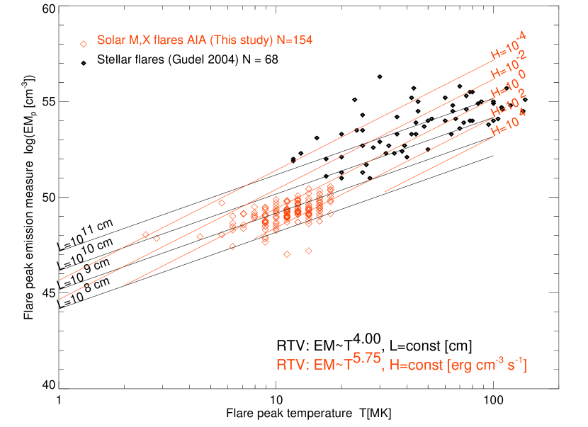
Figure 11: Scatterplot of flare total emission measure $EM_{p}$ versus the flare peak temperature $T_{p}$ for solar and stellar data sets. The predictions of the RTV law are indicated for constant loop lengths $L$ (black lines) and for constant heating rates $H$ (red lines).

A comparison of solar and stellar flare scaling laws has been compiled in Aschwanden, Stern, and Güdel (2008), where an empirical scaling of the peak emission measure $EM_{p}$ with peak temperature $T_{p}$ of $EM_{p}\propto T_{p}^{4.7}$ was found for both populations, but the stellar flares exhibit about a factor of $\approx 250$ times higher emission measures than the solar flares (at the same flare peak temperature). We present a similar scatterplot in Fig. 11, where we sbow the new measurements of the 155 M and X-class flares obtained from AIA/SDO and GOES. In addition we overlay the predicted relationship for the RTV law for both constant loop lengths and constant heating rates. For constant loop lengths, the predicted RTV scaling is $EM_{p}\propto T_{p}^{4}$ (Eq. 17), while a constant heating rate implies $L_{p}\propto T_{p}^{7/4}$ (using Eq. 18), which yields $EM_{p}\propto T_{p}^{5.75}$ (by inserting Eq. 18 into Eq. 17). An alternative relationship of $EM_{p}\propto T_{p}^{8.5}$ was derived for a magnetic reconnection model (Shibata and Yokoyama 1999).

Following the RTV predictions we can see from Fig. 11 that most of the large solar flares are produced with heating rates of $H\approx 10^{-2},...,1$ erg cm^-3 s^-1 on spatial scales of $L_{p}\approx 10^{8}-10^{10}$ Mm. Stellar flares exhibit a higher range of heating rates and also require larger spatial scales of $L\approx 10^{9}-10^{12}$ cm. It appears that the largest stellar flares occupy larger volumes than solar flares, while the smallest detected stellar flares have similar sizes as the largest solar flares.

4.5 Predicting the Largest and Smallest Solar Flare

The scaling laws we established here set a firm upper limit on the largest flare events. The temperature distribution $N(T_{p})$ drops off steeply at $T_{e}\approx 20$ MK (Fig. 2d), so that this value can be considered as an upper limit on temperatures $T_{p}$ as measured at the peak of the DEM distribution function. Spatial scales are found to have a cutoff at $L_{p}\lower 1.72218pt\hbox{$\;\buildrel<\over{\scriptstyle\sim}\;$}7\times 10^{9}$ cm, corresponding to a diameter of $2L_{p}\lower 1.72218pt\hbox{$\;\buildrel<\over{\scriptstyle\sim}\;$}1.4\times 10^{10}$ cm (or 140 Mm), which corresponds to 10% of the solar diameter, which is physically dictated by the maximum size of the largest active regions. The maximum predicted thermal energy in solar flares is thus, $E_{th}=c_{5}T_{p}^{4}L_{p}^{2}\lower 1.72218pt\hbox{$\;\buildrel<\over{\scriptstyle\sim}\;$}3\times 10^{32}$ erg (Eq. 17).

This energy estimate of the largest solar flare possible agrees with a recent study, which states that the largest solar flares observed over the past few decades have reached energies of a few times $10^{32}$ ergs (Aulanier et al. 2013). Alternatively, the same authors estimated the largest amount of released magnetic energy possible from assuming a flare size that covers 30% of the largest sunpspot group ever reported, with its peak magnetic field being set to the strongest value ever measured in a sunspot, which then produces a flare with a maximum magnetic energy of $\approx 6\times 10^{33}$ ergs, which is a factor of 20 higher than the upper limit of thermal energies based on the RTV scaling. However, only a fraction of the magnetic energy is converted into thermal energy, a factor that is estimated to be in the order of $\approx 1\%-10\%$ (Emslie et al. 2004, 2005, 2013).

In the other extreme, we can also predict the energy of the smallest flare using the relationship of Eq. (17). A lower limit for the temperature is given by the background corona, which is approximately $T_{min}=1.0$ MK in active regions. The minimum length scale is given by the smallest loop segment that sticks out of the transition region, which we estimate to $L_{min}\approx 1.0$ Mm, given the chromospheric height of $h\approx 2.0$ Mm. Thus the smallest detectable nanoflare is expected to have a thermal energy of $E_{th}=c_{5}T_{p}^{4}L_{p}^{2}\lower 1.72218pt\hbox{$\;\buildrel>\over{\scriptstyle\sim}\;$}7\times 10^{24}$ erg (Eq. 17), which is almost 8 orders of magnitude smaller than the largest predicted flare and justifies the term nanoflare. Since the dataset analyzed here includes only large flares, extrapolations of the scaling laws to the nanoflare regime may bear large uncertainties, which will be reduced in future studies that include smaller flare events.

4.6 Predicting Powerlaw Distributions for SOC Models

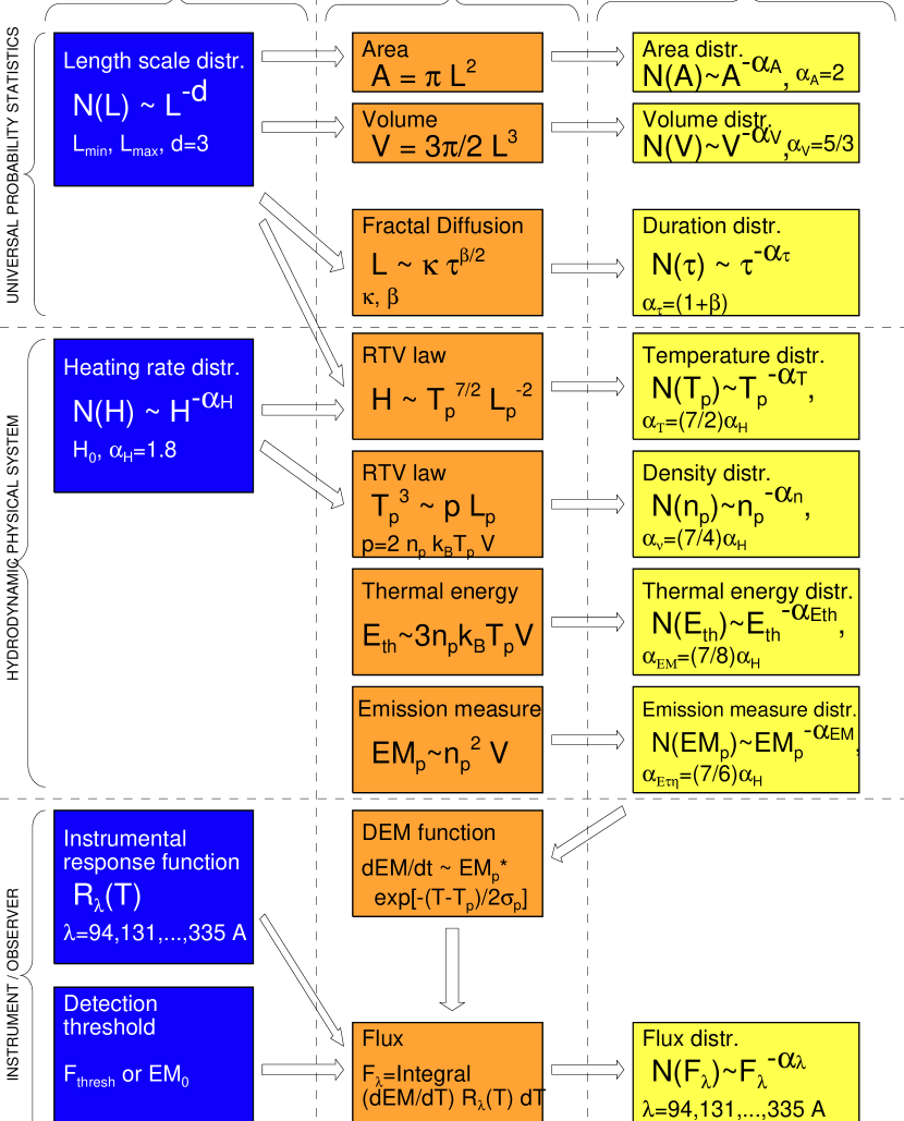
Figure 12: Flow chart of input parameters (left), scaling laws (middle), and output distribution functions (right) of the fractal-diffusive SOC model applied to solar flares. The spatio-temporal parameters ($L,A,V,\tau$) follow from universal probability statistics (top part of diagram), while the physical parameters and their scaling laws are specific to the hydrodynamics of solar flares (middle part of diagram), and the instrumental response functions as a function of temperature and wavelengths are specific to the observer (bottom part of diagram). The given powerlaw indices $\alpha_{x}$ are approximative values for dimensionality $d=3$.

Self-organized criticality (SOC) models can be characterized by powerlaw-like occurrence frequency or size probability distribution functions. After we investigated various scaling laws between observables and inferred physical parameters, the question arises now whether we are able to predict all observed distribution functions with the correct powerlaw slopes from first principles. A diagram of the application of the fractal-diffusive (FD-SOC) model to the physical system of solar flares is provided in Fig. 12, visualized as a flow chart that progresses from the input parameters (left) to the output distribution functions (right) in three different regimes: (i) The spatio-temporal regime that follows from universal statistics (Fig. 12, top part), (ii) the regime of the physical system that is described by the hydrodynamic RTV scaling laws (Fig. 12, middle part), and (iii) the observers regime that is characterized by the response functions and detection sensitivity of a specific instrument (Fig. 12, bottom). From this diagram we can easily see what input parameters are required to predict all output distribution functions: the Euclidean dimension $d$ of the system, limits on the minimum and maximum length scales ($L_{min},L_{max}$), the lower limit $H_{0}$ of the heating rate that triggers a flare instability, the powerlaw index $\alpha_{H}$ of the heating function, the instrumental response functions $R_{\lambda}(T)$, and the flux threshold $F_{thresh}$ or emission measure threshold $EM_{0}$ of the flare event detection algorithm, the diffusion coefficient $\kappa$, the diffusion spreading exponent $\beta$, and the Gaussian width $\sigma_{p}$ of the DEM distribution function, which all have been determined in the present analysis for a representative sample of large (M and X GOES class) flares. The best-fitting values were found to be: $d=3$, $L_{min}=4$ Mm, $L_{max}=70$ Mm, $H_{0}=0.04$ erg cm^-2 s^-1, $\alpha_{H}=1.8$, $EM_{0}=10^{48.5}$ (for GOES M1.0 class level), $\beta=0.53\pm 0.27$, $\kappa\approx 52$ km s^-β/2, $\sigma_{p}=0.50\pm 0.13$. Using these input parameters, we can predict every probability distribution function $N(x)$ for the parameters $x=(L,A,V,\tau,T_{p},n_{p},E_{th},EM_{p})$. In addition, choosing a suitable instrument sensitive to both EUV and soft X-ray wavelengths, we need in addition to know the instrumental response functions $R_{\lambda}(T)$ as a function of the temperature $T$, and can then predict the probability distribution functions $N(F_{\lambda})$ of the flux $F_{\lambda}$ for any arbitrary wavelength channel $\lambda$.

Ultimately, this framework could be developed further, by including scaling laws and distribution functions of the magnetic field $B$, since we expect that the primary energy source of the heating process comes from dissipation of magnetic energy. This requires the knowledge of a scaling law between the heating rate $H(B,L_{p})$ and the magnetic field strength $B$ and length scales $L_{p}$, as tentatively discussed in Appendix B and to be examined in a future study.

5 CONCLUSIONS

While we analyzed the spatio-temporal evolution of a complete set of 155 flares (above the M and X-GOES class level) in Paper I, we conduct a differential emission measure (DEM) analysis on the same set of flares in this Paper II, in order to derive statistics, size distributions, and scaling laws of physical parameters measured during the peak times of the flares, such as electron temperatures, electron densities, emission measures, and thermal energies. The DEM analysis is based on the six coronal wavelength filters of AIA (94, 131, 171, 193, 211, 335), which allow us temperature diagnostics in the range of $T_{e}\approx 1-20$ MK. The quality of the DEM results measured at the flare peak time $t_{p}$ carried out here is comprehensive in wavelength and time coverage, since we carry out DEM fits throughout the flare impulsive phase (in order to detect the emission measure peak time $t_{p}$) and since AIA provides sensitivity in a sufficiently broad temperature range to reliably detect the peak temperature $T_{p}$ at the spectral peak $EM_{p}$ of the DEM. The major conclusions of this statistical study are:

1. The six observed fluxes $F_{\lambda}$ of the coronal wavelength filters of AIA/SDO measured during the soft X-ray peak times $t_{p}$ of virtually all analyzed flares can be fitted with a single-Gaussian differential emission measure (DEM) function, with an average goodness-of-fit of $F_{fit}/F_{obs}=1.13\pm 0.48$. These DEM fits provide the three key parameters of the flare peak emission measure $EM_{p}$, peak temperature $T_{p}$, and Gaussian temperature width $\sigma_{p}$ of the DEM. These parameters were determined in the ranges of $log(EM_{p})=47.0-50.5$, $T_{p}\approx 5.0-17.8$ MK, and $\sigma_{p}=0.22-0.75$ (or $\sigma_{p}=0.50\pm 0.14$).

2. Measuring the time-integrated flare area $A=\pi L_{p}^{2}$ with radius $L_{p}$, assuming a hemispheric flare volume $V=(2/3)\pi L_{p}^{3}$, and a filling factor of unity, we derive the average electron density $n_{p}=\sqrt{(EM_{p}/V)}$ and the thermal energy $E_{th}=3n_{p}k_{B}T_{p}V$ at the flare peak time, which are found in the ranges of $n_{p}=3.8\times 10^{9}-8.8\times 10^{11}$ cm^-3 and $E_{th}=1.6\times 10^{28}-1.1\times 10^{32}$ erg.

3. Using the parameters $L_{p}$, $T_{p}$, and $n_{p}$ we test the RTV scaling law and find an excellent agreement between the RTV-predicted and observed parameters, with a mean of $T_{RTV}/T_{obs}=1.05\pm 0.38$ or $L_{RTV}/L_{obs}=n_{RTV}/n_{obs}=1.3\pm 2.1$. This agreement implies that energy balance between the heating rate and radiative and conductive loss rates is achieved during the flare peak time $t_{p}$, which permits the applicability of the RTV scaling law near this particular time in the flare evolution, although the hydrodynamic evolution is not stationary and the heating is not spatially uniform, as assumed in the original derivation of the RTV scaling law.

4. The RTV scaling laws allow us to calculate the probability distributions of the flare peak temperatures, $N(T_{p})\propto T_{p}^{\alpha_{T}}$, peak electron densities, $N(n_{e})\propto n_{p}^{\alpha_{n}}$, peak emission measures $N(EM_{p})\propto EM_{p}^{\alpha_{EM}}$, and thermal energies $N(E_{th})\propto E_{th}^{\alpha_{Eth}}$, if the size distributions of length scales $N(L_{p})$ and heating rates $N(H)$ are known. The length scale distribution, postulated by the scale-free probability conjecture, $N(L_{p})\propto L_{p}^{-3}$, is found to be consistent with the observations. Assuming a powerlaw function for the heating rates, $N(H)\propto H^{-\alpha_{H}}$, with a slope of $\alpha_{H}=1.8$ and a cutoff at $H\lower 1.72218pt\hbox{$\;\buildrel>\over{\scriptstyle\sim}\;$}H_{0}=0.04$ erg cm^-3 s^-1 yields an accurate match for the observed powerlaw slopes within the uncertainties of the powerlaw fits, i.e., $\alpha_{EM}=1.78\pm 0.03$, $\alpha_{n}=2.15\pm 0.17$, and $\alpha_{Eth}=1.66\pm 0.13$.

5. We show also how the size distributions of $T_{p}$, $n_{p}$, $EM_{p}$, $E_{th}$ can be calculated analytically, using the RTV scaling laws, the truncation effects due to the emission measure or flux threshold, the truncation effects caused by lower heating rate limit, and the lower and upper length scale limit. Using the instrumental response functions $R_{\lambda}(T)$ of a wavelength filter $\lambda$, we can also model the observed fluxes $F_{\lambda}$ in each wavelength $\lambda$, their size distributions (which all turn out to be $N(F_{\lambda})\propto F_{\lambda}^{-2}$), and the high degree of correlations in flux-flux, flux-volume, or flux-emission measure relationships.

6. Our result of the inferred volumetric heating rate size distribution $N(H)\propto H^{-1.8}$ predicts identical size distributions for the magnetic field, $N(B)\propto B^{-1.8}$, and the magnetic fluxes, $N(\Phi)\propto\Phi^{-1.8}$, and is consistent with the statistics of magnetic fluxes on the solar surface measured by Parnell et al. (2009), as well as with the heating flux scaling law $F_{H}=H\times L\propto BL^{-1}$ found from hydrostatic simulations of the entire Sun’s corona by Schrijver et al. (2004).

7. The size distribution of thermal flare energies is found to be $N(E_{th})\propto E_{th}^{1.66\pm 0.13}$, which is close to the size distribution of non-thermal flare energies calculated from hard X-ray producing electrons, $N(E_{nth})\propto E_{nth}^{1.53\pm 0.02}$. This finding of a powerlaw slope below the critical value of 2 corroborates that the energy dissipated in the solar corona is dominated by the largest flares. If this distribution holds down to the smallest energies (which is the subject of future studies), heating of the solar corona by nanoflares can be ruled out. The dataset analyzed here, however, includes only large flares, and thus no conclusion can be drawn about the significance of nanoflares.

8. The RTV scaling law allows us to predict the largest and smallest solar flare, which is estimated to be $E_{th,min}\lower 1.72218pt\hbox{$\;\buildrel>\over{\scriptstyle\sim}\;$}7\times 10^{24}$ erg for the smallest flare, and $E_{th,max}\lower 1.72218pt\hbox{$\;\buildrel<\over{\scriptstyle\sim}\;$}3\times 10^{32}$ erg for the largest flare, spanning a range of almost 8 orders of magnitude in energy. For the analyzed sample of M and X-class flares we find an energy range of 3 orders of magnitude ($E_{th}\approx 10^{29}-10^{32}$ erg).

9. Comparing solar with stellar flares and applying the RTV predictions we find that most of the large solar flares are produced with heating rates of $H\approx 10^{-2},...,10^{2}$ erg cm^-3 s^-1 on spatial scales of $L_{p}\approx 10^{8}-10^{10}$ Mm. Stellar flares exhibit a similar range of heating rates but require larger spatial scales of $L\approx 10^{9}-10^{12}$ cm. It appears that the largest stellar flares occupy larger volumes than solar flares, while the smallest detected stellar flares have similar sizes as the largest solar flares.

This study conveyed deeper physical insights into nonlinear phenomena controlled by self-organized criticality. We have shown that the nonlinear nature of scaling laws generally predicts powerlaw distribution functions for most observables, especially for energy distribution functions, a key parameter to characterize the size of SOC avalanches. Our concept of the fractal-diffusive SOC model (Aschwanden 2012a) provides a framework to relate powerlaw distribution functions and correlations of SOC parameters to physical scaling laws that govern SOC phenomena. For solar flares we found that the hydrodynamic processes can be formulated with the RTV scaling law during the flare peak time, what allowed us to retrieve the size distribution of average heating rates in flares, which turned out to be identical to the magnetic flux distribution (as measured by Parnell et al. 2009). Future studies with measurements of the magnetic field in flare sites are likely to reveal us scaling laws between the magnetic energy dissipation rate and plasma heating in solar flares.

Appendix A: Analytical Calculation of Truncation Effects in Powerlaw Size Distributions using the RTV Law

In this Appendix we calculate quantitatively how truncation effects and incomplete sampling affects the observed powerlaw distributions.

In our study we sampled only flares larger than the GOES M1.0 class, which represents a lower limit of the flux or emission measure. This is also true for most other datasets, since event catalogs are generally compiled with some completeness down to an instrument-dependent flux threshold or a related selection criterion. Thus, we have to calculate how a flux or emission measure threshold, $EM\geq EM_{0}$, scales for each parameter. From Eq. (16) we obtain directly how the length limit $L_{1}$ scales for a fixed threshold value $EM_{0}$ as a function of the temperature $T_{p}$,

$$L_{1}(T_{p})=\left({EM_{0}\over c_{4}}\right)T_{p}^{-4}\ ,$$

or on the electron density $n_{p}$,

$$L_{1}(n_{p})=\left({3\over 2\pi}EM_{0}\right)^{1/3}n_{p}^{-2/3}\ .$$

Similarly, by inserting the thermal energy $E_{th}$ from the RTV scaling law (Eq. 17) we obtain,

$$L_{1}(E_{th})=\left(c_{5}^{4/3}{EM_{0}\over c_{4}}\right)^{-3/5}E_{th}^{4/5}\ ,$$

or for the heating rate $H$ (Eq. 18),

$$L_{1}(H)=\left({c_{6}^{8/7}EM_{0}\over c_{4}}\right)^{7/23}H^{-8/23}\ .$$

These truncation boundaries are overplotted onto the scatterplots of the observables $L_{p}$ versus $T_{p}$, $n_{p}$, $H_{p}$, $EM_{p}$, and $E_{th}$ in Fig. 7 (dashed lines). We see that these truncation boundaries constitute a lower limit of length scales $L_{1}$ for the parameters $T_{p}$, $n_{p}$, and $H_{p}$, but an upper limit of length scales $L_{1}$ for the thermal energies $E_{th}$. These length scale limits $L_{1}$ quantify the undersampling and threshold effects due to a lower emission measure limit or instrumental flux detection threshold, which we have to implement in the analytical derivation of the size distributions and powerlaw slopes.

The lower cutoff $H_{0}$ of the heating rate distribution causes also truncation effects, as it can be seen in the scatterplots in Fig. 7 (dotted linestyle). We calculate how the heating rate cutoff $H\geq H_{0}$ scales with each parameter. From Eq. (18) we obtain directly how the length limit $L_{2}$ scales for a fixed heating rate value $H_{0}$ as a function of the temperature $T_{p}$,

$$L_{2}(T_{p})=\left({c_{6}\over H_{0}}\right)^{1/2}T_{p}^{7/4}\ ,$$

or on the electron density $n_{p}$ (using Eqs. 18 and 14),

$$L_{2}(n_{p})=\left({c_{6}c_{1}^{7/2}\over H_{0}}\right)^{4}n_{p}^{7}\ .$$

Similarly, by inserting the peak emission measure $EM_{p}$ from the RTV scaling law (Eqs. 16 and 18) we obtain,

$$L_{2}(EM_{p})=\left({c_{6}\over H_{0}c_{4}^{7/8}}\right)^{8/23}EM_{p}^{7/23}\ ,$$

or for the thermal energy $H$ (Eqs. 17 and 18),

$$L_{2}(E_{th})=\left({c_{6}\over H_{0}c_{5}^{7/6}}\right)^{3/13}E_{th}^{7/26}\ .$$

These truncation boundaries are overplotted onto the scatterplots of the observables $L_{p}$ versus $T_{p}$, $n_{p}$, $H_{p}$, $EM_{p}$, and $E_{th}$ in Fig. 7 (dotted lines). We see that these truncation boundaries constitute an upper limit of length scales $L_{2}$ for the parameters $T_{p}$, $n_{p}$, $EM_{p}$, and $E_{th}$. These length scale limits $L_{2}$ affect the size distributions in those regimes where $L_{2}<L_{max}$, which we have to consider in the calculation of the size distributions in the next subsection.

Using the two size distributions $N(L_{p})$ (Eq. 19) and $N(H)$ (Eq. 20), we can calculate analytically the predicted size distributions $N(x)dx$ for all physical parameters $x=T_{p},n_{p},EM_{p},E_{th},H_{p}$, by integrating the length scale distribution $N(L)$ from the minimum $L_{1}(x)$ to the maximum value $L_{2}(x)$, and by substituting the parameters $x$ according to the RTV scaling law relationships given in Eqs. (13-18),

$$N(x)=\int_{L_{1}(x)}^{L_{2}(x)}N(L,H,x)\ dL=\int_{L_{1}(x)}^{L_{2}(x)}N(L)\ N(H[L,x])\ dL=\int_{L_{1}(x)}^{L_{2}(x)}N_{0}\ L^{-3}H[L,x]^{-\alpha_{H}}\ dL\ ,$$

where the integration boundaries $L_{1}(x)$ and $L_{2}(x)$ have to be adjusted to the cutoffs $L_{1}(x)$ (Eqs. A1-A4) imposed by the emission measure threshold $EM_{0}$ and the cutoffs $L_{2}(x)$ set by the minimum heating rate $H_{0}$ (Eqs. A5-A8).

We start with the occurrence frequency of temperatures $N(T_{p})$, for which we obtain,

$$N(T_{p})\propto\int_{L_{1}(T_{p})}^{L_{2}(T_{p})}T^{-(7/2)\alpha_{H}}\ L_{p}^{-3+2\alpha_{H}}\ dL\propto T^{-(7/2)\alpha_{H}}\ \left[-L_{2}(T_{p})^{2(\alpha_{H}-1)}+L_{1}(T_{p})^{2(\alpha_{H}-1)}\right]\ ,$$

where the minimum temperature $T_{min}$ is defined by the intersection point of the emission measure threshold $L_{1}(T_{p})$ (Eq. A1) with the heating threshold $L_{1}(H)$ (Eq. A4), at

$$T_{p}\geq T_{min}=\left[\left({EM_{0}\over c_{4}}\right)\left({H_{0}\over c_{6}}\right)^{1/2}\right]^{4/23}\ ,$$

which amounts to $T_{min}=5.25$ MK for our model with $EM_{0}=10^{48.5}$ cm^-3 and $H_{0}=0.04$ erg cm^-3. The lower integration limit is given either by the emission measure threshold limit at $L_{1}(T_{p},EM_{0})$ (Eq. A1) or the length scale minimum $L_{min}$, while the upper integration limit is given by the heating rate limit $L_{2}(T_{p},H_{0})$ (Eq. A5) or the length scale maximum $L_{max}$, which are all indicated in the Figs. 6 and 8 (panels b). The so obtained analytical function of the temperature distribution $N(T_{p})$ is shown in Fig. 9b (red curve), which is confined to a narrow range that increases from $T_{min}=5.25$ MK steeply to a maximum at $T_{e}=8.85$ MK, and drops again steeply in the range of $T_{e}=8.85-20$ MK to the sensitivity limit of the AIA instrument.

The second distribution we are going to calculate is for the electron peak density, $N(n_{p})$. Again, by inserting the heating rate relationship $H(T_{p},L_{p})$ (Eq. 18) and the RTV relationship $T_{p}\propto(n_{p}L_{p})^{1/2}$ (Eq. 13) into the general distribution $N(x)$ (Eq. A9) with $x=n_{p}$, we predict the following density distribution $N(n_{p})$,

$$N(n_{p})\propto\int_{L_{1}(n_{p})}^{L_{2}(n_{p})}n_{p}^{-(7/4)\alpha_{H}}\ L_{p}^{-3+\alpha_{H}/4}\ dL\propto n_{p}^{-(7/4)\alpha_{H}}\ \left[-L_{2}(n_{p})^{-2+\alpha_{H}/4}+L_{1}(T_{p})^{-2+\alpha_{H}/4}\right]\ ,$$

where the minimum density $n_{min}$ is defined by the intersection point of the emission measure threshold $L_{1}(n_{p})$ (Eq. A2) with the heating threshold $L_{1}(n_{p})$ (Eq. A2), at

$$n_{p}\geq n_{min}=\left[\left({{3\over 2\pi}EM_{0}}\right)^{1/3}\left({H_{0}\over c_{6}c_{1}^{7/2}}\right)^{4}\right]^{3/16}\ ,$$

which amounts to $n_{min}=8.25\times 10^{9}$ cm^-3 for our model with $EM_{0}=10^{48.5}$ cm^-3 and $H_{0}=0.04$ erg cm^-3. The lower integration limit is given either by the emission measure threshold limit at $L_{1}(n_{p},EM_{0})$ (Eq. A2) or the length scale minimum $L_{min}$, while the upper integration limit is given by the heating rate limit $L_{2}(n_{p},H_{0})$ (Eq. A6) or the length scale maximum $L_{max}$, which are all indicated in the Figs. 7c and 8c. The so obtained analytical function of the density distribution $N(n_{p})$ is shown in Fig. 9c (red curve),

The third distribution we are calculating is the emission measure distribution $N(EM)$, by inserting the RTV relationships for $H(T_{p},L_{p})$ (Eq. 18) and $T_{p}(EM_{p},L_{p})$ (Eq. 13) into the general distribution $N(x)$ (Eq. A9) with $x=EM_{p}$,

$$N(EM_{p})\propto\int_{L_{1}(EM_{p})}^{L_{2}(EM_{p})}EM_{p}^{-(7/8)\alpha_{H}}\ L_{p}^{-3+(23/8)\alpha_{H}}\ dL\propto EM_{p}^{-(7/8)\alpha_{H}}\ \left[-L_{2}(EM_{p})^{-2+(23/8)\alpha_{H}}+L_{min}^{-2+(23/8)\alpha_{H}}\right]\ ,$$

where the lower integration limit is given either by the length scale minimum $L_{min}$, while the upper integration limit is given by the heating rate limit $L_{2}(EM_{p},H_{0})$ (Eq. A7) or the length scale maximum $L_{max}$, which are all indicated in the Figs. 7e and 8e. The so obtained analytical function of the emission measure distribution $N(EM_{p})$ is shown in Fig. 9e (red curve), which represents a powerlaw function with a slope of $\alpha_{EM}=1.73\pm 0.07$.

Similarly we calculate the distribution of thermal energies $N(E_{th})$, by inserting the RTV relationships for $H(T_{p},L_{p})$ (Eq. 18) and $T_{p}(E_{th},L_{p})$ (Eq. 17) into the general distribution $N(x)$ (Eq. A9) with $x=E_{th}$ and predict the following distribution for $N(E_{th})$,

$$N(E_{th})\propto\int_{L_{1}(E_{th})}^{L_{2}(E_{th})}E_{th}^{-(7/6)\alpha_{H}}\ L_{p}^{-3+(13/3)\alpha_{H}}\ dL\propto E_{th}^{-(7/6)\alpha_{H}}\ \left[-L_{2}(E_{th})^{-2+(13/3)\alpha_{H}}+L_{min}^{-2+(13/3)\alpha_{H}}\right]\ ,$$

where the lower integration limit is given by the length scale minimum $L_{min}$, while the upper integration limit is given by the emission measure threshold at $L_{1}(E_{th})$ (Eq. A3), the heating rate limit $L_{2}(E_{th},H_{0})$ (Eq. A8), or the length scale maximum $L_{max}$, which are all indicated in the Figs. 7f and 8f. The so obtained analytical function of the emission measure distribution $N(E_{th})$ is shown in Fig. 8f (red curve), which represents a powerlaw function with a slope of $\alpha_{EM}=1.64\pm 0.06$.

The analytically calculated size distributions (shown in Fig. 8, red curves) exhibit approximate powerlaw functions, as well as slight changes in the slopes and turnover points, all caused by truncations in the datapoints due to the emission measure threshold $EM_{0}$ and the heating rate limit $H_{0}$. For sake of simplicity we used an exact powerlaw distribution of length scales $N(L)\propto L^{-3}$ in the analytical calculations, which neglects truncation effects for small length scales $L$, and thus shows some deviations from the numerically simulated distributions in Fig. 8. More accurate size distributions are obtained with the Monte-Carlo simulations shown in Fig. 8, which compares favorably with the observed values shown in Fig. 7. In particular we match the powerlaw slopes of heating rates ($\alpha_{H}^{obs}=1.45\pm 0.05$ versus $\alpha_{H}^{sim}=1.47\pm 0.09$), for peak emission measures, ($\alpha_{EM}^{obs}=1.78\pm 0.03$ versus $\alpha_{EM}^{sim}=1.73\pm 0.07$), and for thermal energies, ($\alpha_{Eth}^{obs}=1.66\pm 0.13$ versus $\alpha_{Eth}^{sim}=1.64\pm 0.06$). The satisfactory match within the stated uncertainties corroborates the validity of our numerical and analytical models.

Appendix B: Scaling Law of the Coronal Heating Rate

For the heating rate distribution $N(H)\propto H^{-\alpha_{H}}$ (Eq. 20) we made the assumption of a powerlaw function with an unknown powerlaw exponent $\alpha_{H}$, which turned out to require a value of $\alpha_{H}=1.8$ in Monte-Carlo simulations in order to reproduce the observed distributions of $\alpha_{H}^{obs}=1.45$, $\alpha_{n}=2.15$, $\alpha_{EM}=1.78$, and $\alpha_{Eth}=1.66$ (Fig. 7c-f). Can we explain this particular value with a physical model from first principles?

The heating flux $F_{H}$ into active region loops has been statistically determined from hydrostatic simulations of the entire Sun’s corona (Schrijver et al. (2004) and the following scaling law was found between the magnetic field strengths $B$ and the loop length $L$,

$$F_{H}\propto B^{1.0\pm 0.3}L^{-1.0\pm 0.5}\approx BL^{-1}\ .$$

The heating flux $F_{H}$ represents the energy flux (in units or erg cm^-2 s^-1) per footpoint area of a loop. From the heat flux $F_{H}$ we can deduce the following scaling law for the average volumetric heating rate $H=F_{H}/L$,

$$H\propto{F_{H}\over L}\propto BL^{-2}\ .$$

Substituting this scaling law relationship $H(B,L)$ into the generalized size distribution $N(x)$ (Eq. A9) with $x=B$, we can derive the size distribution of magnetic fields for loops or flares in the solar corona,

$$N(B)\propto\int N(L)N(H[B,L])dL\propto\int L^{-3}(BL^{-2})^{-\alpha_{H}}dL\propto B^{-\alpha_{H}}\left[L^{-2+2\alpha_{H}}\right]_{L,min}^{L_{max}}\ ,$$

which essentially yields a size distribution $N(B)\propto B^{-1.8}$ that is identical to the heating rate distribution $N(H)\propto H^{-1.8}$, if we neglect truncation effects (as discussed in Appendix A).

Besides this prediction for the size distributions of magnetic fields, we can also predict the size distribution for magnetic fluxes $\Phi$ of active regions or flaring regions with size $A\propto L^{2}$, which are defined by the following scaling law,

$$\Phi=\int_{A}B(x,y)dxdy=B\ A\propto B\ L^{2}\ .$$

Substituting this variable of the magnetic flux $\Phi$ into the volumetric heating rate scaling law $H\propto BL^{-2}$ (Eq. B2), we have a scaling law of the heating rate $H$ as a function of the variables $\Phi$ and $L$,

$$H\propto BL^{-2}\propto\Phi L^{-4}\ ,$$

and can then derive the size distribution $N(\Phi)$ of magnetic fluxes by substituting this scaling law $H(\Phi,L)$ into the generalized size distribution $N(x)$ (Eq. A9) with $x=\Phi$, which yields,

$$N(\Phi)\propto\int N(L)N(H[\Phi,L])dL\propto\int L^{-3}(\Phi L^{-4})^{-\alpha_{H}}dL\propto\Phi^{-\alpha_{H}}\left[L^{-2+2\alpha_{H}}\right]_{L,min}^{L_{max}}\ ,$$

which essentially yields a size distribution $N(\Phi)\propto\Phi^{-1.8}$ that is identical to the magnetic field distribution $N(B)\propto B^{-1.8}$ or the heating rate distribution $N(H)\propto H^{-1.8}$, if we neglect truncation effects (as discussed in Appendix A). This prediction actually agrees with recent statistical observations of the magnetic flux on the solar surface, which was found to be distributed as a powerlaw distribution over more than five decades in flux (Parnell et al. 2009),

$$N(\Phi)\propto\Phi^{-1.85\pm 0.14}\ ,$$

based on magnetic features distributed all over the Sun, using SohO/MDI and Hinode/SOT data. A coupling between the size distribution of photospheric magnetic features and coronal energy dissipation events was also established in a recent study (Uritsky et al. 2013). Thus our result of the inferred volumetric heating rate size distribution $N(H)\propto H^{-1.8}$ is consistent with the statistics of magnetic fluxes on the solar surface measured by Parnell et al. (2009), as well as with the heating flux scaling law $F_{H}=H/L\propto BL^{-1}$ found from hydrostatic simulations of the entire Sun’s corona by Schrijver et al. (2004).

Table 1: Statistics of powerlaw slopes $\alpha_{F}$ of AIA fluxes $F_{\lambda}$ 155 solar flares, tabulated in 7 AIA wavelengths and for 5 different flux thresholds. The theoretical prediction of the FD-SOC model is $\alpha_{F}=2.0$.

Wavelength	Threshold	Threshold	Threshold	Threshold	Threshold	All
[$\AA$]	1%	2%	5%	10%	20%
94	2.2	2.2	2.2	2.2	2.1	2.2$\pm$ 0.04
131	2.0	2.0	2.0	2.0	2.0	2.0$\pm$ 0.02
171	2.1	1.9	2.0	2.0	2.2	2.0$\pm$ 0.1
193	2.1	2.0	2.1	2.1	1.9	2.0$\pm$ 0.1
211	2.3	2.1	2.1	2.2	2.0	2.1$\pm$ 0.1
304	2.1	2.1	1.9	2.5	2.0	2.1$\pm$ 0.2
335	1.8	2.1	2.1	1.8	1.9	1.9$\pm$ 0.1
All	2.1$\pm$ 0.2	2.1$\pm$ 0.1	2.1$\pm$ 0.1	2.1$\pm$ 0.2	2.0$\pm$ 0.1	2.1$\pm$ 0.1

Table 2: Catalog of 155 analyzed M and X-class flare events and best-fit model parameters: length scale $L_{p}$(Mm), electron temperature $T_{p}$ (MK), Gaussian temperature width of DEM peak $\sigma_{p}$, electron density $n_{p}$ (cm^-3), emission measure peak $EM_{p}$ (cm^-3), thermal energy $E_{th}$ (erg), and ratio of DEM-fitted to observed flux $F_{fit}/F_{obs}$ at the peak time of the flares.

Nr	Observation	Peak	GOES	Length	Temperature	Temperature	Electron	Emission	Thermal	DEM
	date	time	class	scale	peak	width	density	measure	energy	fit
		HH:MM		$L_{p}$ (Mm)	$T_{p}$ (MK)	$log(\sigma_{p})$	$\log(n_{e})$	$\log(EM_{p})$	$\log(E_{th})$	$F_{fit}/F_{obs}$
1	2010-06-12	00:58	M2.0	21	14.1	0.50	10.6	49.3	30.7	0.96$\pm$0.26
2	2010-06-13	05:39	M1.0	16	12.6	0.59	10.9	49.3	30.6	1.18$\pm$0.46
3	2010-08-07	18:24	M1.0	38	7.9	0.65	10.1	48.9	30.7	1.57$\pm$0.94
4	2010-10-16	19:12	M2.9	25	15.8	0.59	10.8	49.9	31.2	1.01$\pm$0.14
5	2010-11-04	23:58	M1.6	15	10.0	0.60	10.5	48.5	30.0	1.37$\pm$0.83
6	2010-11-05	13:29	M1.0	19	11.2	0.36	10.7	49.2	30.6	1.27$\pm$0.43
7	2010-11-06	15:36	M5.4	17	14.1	0.34	9.6	47.2	29.4	0.86$\pm$0.28
8	2011-01-28	01:03	M1.3	24	11.2	0.53	10.6	49.0	30.8	1.08$\pm$0.38
9	2011-02-09	01:31	M1.9	17	7.1	0.66	10.6	49.1	30.1	1.25$\pm$0.58
10	2011-02-13	17:38	M6.6	35	14.1	0.47	10.7	49.9	31.4	1.02$\pm$0.07
11	2011-02-14	17:26	M2.2	15	2.5	0.71	9.9	48.0	28.8	1.10$\pm$0.83
12	2011-02-15	01:56	X2.2	16	17.8	0.50	11.5	50.4	31.3	1.07$\pm$0.14
13	2011-02-16	01:39	M1.0	12	15.8	0.37	11.1	49.1	30.5	1.13$\pm$0.37
14	2011-02-16	07:44	M1.1	11	14.1	0.52	11.0	49.1	30.3	0.90$\pm$0.24
15	2011-02-16	14:25	M1.6	13	12.6	0.70	11.3	49.7	30.7	1.03$\pm$0.14
16	2011-02-18	10:11	M6.6	20	8.9	0.71	10.5	49.1	30.3	0.81$\pm$0.46
17	2011-02-18	10:26	M1.0	29	7.9	0.69	10.4	49.0	30.6	1.04$\pm$0.42
18	2011-02-18	13:03	M1.4	16	4.5	0.67	10.3	47.9	29.5	0.88$\pm$0.70
19	2011-02-18	14:08	M1.0	18	8.9	0.41	10.4	48.7	30.1	1.49$\pm$0.98
20	2011-02-18	21:04	M1.3	7	14.1	0.55	10.9	49.2	29.7	1.11$\pm$0.36
21	2011-02-24	07:35	M3.5	8	14.1	0.22	11.3	49.4	30.2	1.44$\pm$0.86
22	2011-02-28	12:52	M1.1	14	12.6	0.50	11.0	49.3	30.5	0.98$\pm$0.22
23	2011-03-07	05:13	M1.2	21	12.6	0.56	10.7	49.3	30.7	1.01$\pm$0.22
24	2011-03-07	07:54	M1.5	4	14.1	0.51	11.4	49.1	29.4	1.14$\pm$0.44
25	2011-03-07	08:07	M1.4	36	12.6	0.49	10.5	49.2	31.2	1.04$\pm$0.48
26	2011-03-07	09:20	M1.8	11	11.2	0.22	10.2	47.0	29.3	1.03$\pm$0.93
27	2011-03-07	14:30	M1.9	25	8.9	0.40	10.7	49.4	30.8	1.19$\pm$0.44
28	2011-03-07	20:12	M3.7	63	10.0	0.24	10.4	49.6	31.7	1.27$\pm$0.44
29	2011-03-07	21:50	M1.5	12	10.0	0.71	11.0	49.2	30.2	1.06$\pm$0.13
30	2011-03-08	02:29	M1.3	9	6.3	0.73	11.1	49.0	29.8	1.00$\pm$0.14
31	2011-03-08	03:58	M1.5	16	8.9	0.64	10.6	49.0	30.2	1.30$\pm$0.80
32	2011-03-08	10:44	M5.3	28	17.8	0.55	10.8	49.8	31.3	1.01$\pm$0.13
33	2011-03-08	18:28	M4.4	10	14.1	0.25	11.2	49.3	30.4	0.91$\pm$0.20
34	2011-03-08	20:16	M1.4	12	10.0	0.65	10.3	48.4	29.6	0.69$\pm$0.42
35	2011-03-09	11:07	M1.7	32	5.6	0.69	10.3	48.0	30.5	1.07$\pm$0.87
36	2011-03-09	14:02	M1.7	18	10.0	0.55	10.4	48.3	30.2	1.01$\pm$0.48
37	2011-03-09	23:23	X1.5	16	17.8	0.46	11.5	50.4	31.3	1.09$\pm$0.26
38	2011-03-10	22:41	M1.1	8	8.9	0.72	10.6	47.9	29.3	1.03$\pm$0.50
39	2011-03-12	04:43	M1.3	14	11.2	0.53	11.2	49.4	30.7	0.97$\pm$0.25
40	2011-03-14	19:52	M4.2	8	17.8	0.54	11.5	49.8	30.4	1.03$\pm$0.06
41	2011-03-15	00:22	M1.0	6	10.0	0.73	11.2	49.0	29.6	1.00$\pm$0.25
42	2011-03-23	02:17	M1.4	12	14.1	0.49	11.1	49.4	30.5	1.05$\pm$0.11
43	2011-03-24	12:07	M1.0	12	10.0	0.62	11.2	49.3	30.4	0.99$\pm$0.09
44	2011-03-25	23:22	M1.0	14	11.2	0.36	10.8	49.2	30.4	1.12$\pm$0.31
45	2011-04-15	17:12	M1.3	7	11.2	0.55	11.1	48.9	29.7	0.93$\pm$0.40
46	2011-04-22	04:57	M1.8	14	11.2	0.33	11.0	49.3	30.5	1.14$\pm$0.40
47	2011-04-22	15:53	M1.2	11	15.8	0.60	11.3	49.4	30.6	1.02$\pm$0.19
48	2011-05-28	21:50	M1.1	24	12.6	0.52	10.7	49.2	30.9	1.14$\pm$0.31
49	2011-05-29	10:33	M1.4	16	8.9	0.64	10.7	48.8	30.3	1.30$\pm$0.88
50	2011-06-07	06:41	M2.5	52	7.1	0.63	10.2	49.2	31.2	0.70$\pm$0.49
51	2011-06-14	21:47	M1.3	25	12.6	0.50	10.6	49.3	30.8	0.97$\pm$0.26
52	2011-07-27	16:07	M1.1	24	11.2	0.25	10.4	48.9	30.6	1.18$\pm$0.48
53	2011-07-30	02:09	M9.3	35	15.8	0.55	10.7	50.2	31.5	1.00$\pm$0.10
54	2011-08-02	06:19	M1.4	34	10.0	0.37	10.4	49.3	30.9	1.15$\pm$0.40
55	2011-08-03	03:37	M1.1	25	12.6	0.40	10.6	49.2	30.8	1.17$\pm$0.35
56	2011-08-03	04:32	M1.7	31	12.6	0.70	10.6	49.6	31.1	0.98$\pm$0.10
57	2011-08-03	13:48	M6.0	37	12.6	0.42	10.6	49.9	31.3	1.09$\pm$0.36
58	2011-08-04	03:57	M9.3	45	12.6	0.46	10.6	50.1	31.7	1.09$\pm$0.22
59	2011-08-08	18:10	M3.5	28	11.2	0.53	10.6	49.4	30.9	0.95$\pm$0.35
60	2011-08-09	03:54	M2.5	24	14.1	0.46	10.7	49.4	30.9	1.02$\pm$0.17
61	2011-08-09	08:05	X6.9	9	17.8	0.46	11.9	50.6	31.1	1.05$\pm$0.23
62	2011-09-04	11:45	M3.2	21	15.8	0.36	10.8	49.3	30.9	1.42$\pm$0.70
63	2011-09-05	04:28	M1.6	22	8.9	0.38	10.3	48.7	30.2	1.28$\pm$0.79
64	2011-09-05	07:58	M1.2	18	8.9	0.59	10.4	48.5	30.1	1.20$\pm$0.81
65	2011-09-06	01:50	M5.3	29	14.1	0.45	10.7	49.8	31.2	1.06$\pm$0.17
66	2011-09-06	22:20	X2.1	50	14.1	0.59	10.6	50.2	31.8	1.05$\pm$0.32
67	2011-09-07	22:38	X1.8	57	15.8	0.56	10.6	50.3	32.0	0.99$\pm$0.08
68	2011-09-08	15:46	M6.7	42	15.8	0.57	10.6	50.0	31.7	1.05$\pm$0.22
69	2011-09-09	06:11	M2.7	22	14.1	0.41	10.8	49.6	31.0	1.37$\pm$0.73
70	2011-09-09	12:49	M1.2	26	12.6	0.51	10.7	49.3	31.0	1.18$\pm$0.47
71	2011-09-10	07:40	M1.1	23	11.2	0.62	10.6	49.0	30.7	0.90$\pm$0.47
72	2011-09-21	12:23	M1.8	23	12.6	0.65	10.4	48.7	30.5	1.25$\pm$0.66
73	2011-09-22	10:00	M1.1	10	14.1	0.49	11.1	48.9	30.3	1.11$\pm$0.62
74	2011-09-22	11:01	X1.4	22	17.8	0.39	11.1	50.2	31.4	0.96$\pm$0.22
75	2011-09-23	01:59	M1.6	22	14.1	0.41	10.6	49.1	30.7	1.24$\pm$0.50
76	2011-09-23	22:15	M1.6	9	11.2	0.29	11.0	49.0	29.9	1.10$\pm$0.29
77	2011-09-23	23:56	M1.9	32	11.2	0.55	10.6	49.3	31.1	1.08$\pm$0.22
78	2011-09-24	09:40	X1.9	10	17.8	0.45	11.9	50.0	31.1	1.04$\pm$0.34
79	2011-09-24	13:20	M7.1	27	11.2	0.30	10.9	49.7	31.2	1.06$\pm$0.21
80	2011-09-24	16:59	M1.7	19	12.6	0.22	10.5	48.7	30.4	1.09$\pm$0.39
81	2011-09-24	17:25	M3.1	7	7.1	0.68	10.9	48.4	29.3	1.45$\pm$0.65
82	2011-09-24	18:15	M2.8	14	11.2	0.45	11.0	49.0	30.5	1.12$\pm$0.35
83	2011-09-24	19:21	M3.0	17	12.6	0.34	11.0	49.4	30.8	1.09$\pm$0.27
84	2011-09-24	20:36	M5.8	6	15.8	0.47	11.4	49.5	29.9	1.34$\pm$0.75
85	2011-09-24	21:27	M1.2	10	6.3	0.62	10.8	48.5	29.6	1.22$\pm$0.86
86	2011-09-24	23:58	M1.0	15	8.9	0.68	10.3	47.8	29.8	0.66$\pm$0.49
87	2011-09-25	02:33	M4.4	5	14.1	0.36	11.1	48.6	29.5	1.23$\pm$0.51
88	2011-09-25	04:50	M7.4	19	12.6	0.36	11.0	49.8	30.9	1.10$\pm$0.18
89	2011-09-25	08:49	M3.1	5	15.8	0.54	11.4	49.3	29.8	1.11$\pm$0.27
90	2011-09-25	09:35	M1.5	9	1.3	0.23	10.3	47.0	28.2	4.82$\pm$8.82
91	2011-09-25	15:33	M3.7	16	11.2	0.71	11.2	49.8	30.8	1.03$\pm$0.15
92	2011-09-25	16:58	M2.2	7	14.1	0.44	11.2	49.3	30.0	1.07$\pm$0.14
93	2011-09-26	05:08	M4.0	10	15.8	0.54	11.5	49.8	30.8	0.98$\pm$0.12
94	2011-09-26	14:46	M2.6	21	12.6	0.69	11.2	49.9	31.2	1.07$\pm$0.13
95	2011-09-28	13:28	M1.2	12	12.6	0.74	11.2	49.6	30.5	1.04$\pm$0.16
96	2011-09-30	19:06	M1.0	11	10.0	0.32	10.9	49.0	30.0	1.13$\pm$0.26
97	2011-10-01	09:59	M1.2	40	8.9	0.39	10.5	49.3	31.2	1.22$\pm$0.41
98	2011-10-02	00:50	M3.9	13	15.8	0.41	11.5	49.7	31.0	1.02$\pm$0.19
99	2011-10-02	17:23	M1.3	8	7.9	0.75	11.2	49.2	29.9	0.98$\pm$0.16
100	2011-10-20	03:25	M1.6	21	2.8	0.68	10.4	47.9	29.8	1.33$\pm$0.81
101	2011-10-21	13:00	M1.3	11	8.9	0.66	11.1	49.1	30.1	1.20$\pm$0.79
102	2011-10-22	11:10	M1.3	35	6.3	0.64	9.8	48.6	30.2	1.06$\pm$0.80
103	2011-10-31	15:08	M1.1	6	8.9	0.64	10.5	47.7	28.7	0.85$\pm$0.71
104	2011-10-31	18:08	M1.4	14	11.2	0.22	10.7	48.7	30.2	0.89$\pm$0.38
105	2011-11-02	22:01	M4.3	6	15.8	0.45	11.4	49.6	30.0	1.35$\pm$0.78
106	2011-11-03	11:11	M2.5	6	15.8	0.40	11.4	49.4	30.0	1.33$\pm$0.47
107	2011-11-03	20:27	X1.9	10	15.8	0.56	11.7	50.2	30.9	1.08$\pm$0.26
108	2011-11-03	23:36	M2.1	16	8.9	0.64	10.4	48.3	30.0	1.07$\pm$0.82
109	2011-11-04	20:40	M1.0	8	15.8	0.39	11.0	49.0	30.0	1.35$\pm$0.59
110	2011-11-05	03:35	M3.7	25	14.1	0.38	10.6	49.6	30.9	1.11$\pm$0.27
111	2011-11-05	11:21	M1.1	15	14.1	0.50	10.6	48.8	30.3	1.31$\pm$0.92
112	2011-11-05	20:38	M1.8	13	12.6	0.42	11.1	49.2	30.5	0.99$\pm$0.16
113	2011-11-06	01:03	M1.2	10	11.2	0.71	11.0	49.2	30.1	0.99$\pm$0.13
114	2011-11-06	06:35	M1.4	14	12.6	0.37	11.0	49.2	30.5	1.12$\pm$0.23
115	2011-11-09	13:35	M1.1	50	7.9	0.31	10.2	49.1	31.2	1.26$\pm$0.75
116	2011-11-15	09:12	M1.2	8	11.2	0.46	11.2	49.0	29.9	1.01$\pm$0.14
117	2011-11-15	12:43	M1.9	9	12.6	0.45	11.3	49.5	30.2	1.11$\pm$0.27
118	2011-11-15	22:35	M1.1	18	10.0	0.49	10.7	48.6	30.4	1.05$\pm$0.41
119	2011-12-25	18:16	M4.0	26	12.6	0.65	10.7	49.7	31.0	1.03$\pm$0.34
120	2011-12-26	02:27	M1.5	17	11.2	0.26	10.7	49.0	30.4	1.05$\pm$0.27
121	2011-12-26	20:30	M2.3	21	14.1	0.46	10.8	49.5	30.9	0.97$\pm$0.23
122	2011-12-29	13:50	M1.9	16	14.1	0.56	10.9	49.2	30.6	1.37$\pm$0.89
123	2011-12-29	21:51	M2.0	14	12.6	0.59	10.9	49.2	30.3	1.20$\pm$0.69
124	2011-12-30	03:09	M1.2	12	11.2	0.64	10.8	48.9	30.1	0.89$\pm$0.42
125	2011-12-31	13:15	M2.4	17	10.0	0.58	10.6	48.9	30.3	1.08$\pm$0.56
126	2011-12-31	16:26	M1.5	22	11.2	0.48	10.6	49.2	30.6	1.15$\pm$0.37
127	2012-01-14	13:18	M1.4	12	6.3	0.58	10.5	48.3	29.5	1.28$\pm$0.79
128	2012-01-17	04:53	M1.0	22	10.0	0.58	10.7	49.2	30.7	1.03$\pm$0.27
129	2012-01-18	19:12	M1.7	31	14.1	0.54	10.5	49.4	31.1	0.95$\pm$0.30
130	2012-01-19	16:05	M3.2	44	8.9	0.24	10.2	49.5	31.1	1.09$\pm$0.40
131	2012-01-23	03:59	M8.7	45	15.8	0.39	10.5	50.0	31.6	1.20$\pm$0.55
132	2012-01-27	18:37	X1.7	51	10.0	0.41	10.4	49.9	31.5	1.07$\pm$0.54
133	2012-02-06	20:00	M1.0	31	11.2	0.56	10.3	49.4	30.8	0.97$\pm$0.36
134	2012-03-02	17:46	M3.3	16	17.8	0.30	10.7	49.1	30.5	1.01$\pm$0.63
135	2012-03-04	10:52	M2.0	21	12.6	0.23	10.7	49.1	30.7	1.15$\pm$0.57
136	2012-03-05	04:09	X1.1	43	10.0	0.41	10.4	49.7	31.3	1.13$\pm$0.54
137	2012-03-05	19:16	M2.1	16	11.2	0.59	10.7	49.0	30.4	1.02$\pm$0.45
138	2012-03-05	19:30	M1.8	17	10.0	0.57	10.8	48.7	30.5	1.05$\pm$0.67
139	2012-03-05	22:34	M1.3	14	6.3	0.61	10.0	47.4	29.2	1.49$\pm$0.89
140	2012-03-06	00:28	M1.3	15	8.9	0.45	10.6	48.7	30.0	1.54$\pm$0.90
141	2012-03-06	01:44	M1.2	13	8.9	0.62	10.7	48.7	30.0	1.03$\pm$0.48
142	2012-03-06	04:05	M1.0	18	7.1	0.66	10.5	48.6	30.1	1.23$\pm$0.45
143	2012-03-06	07:55	M1.0	17	8.9	0.47	10.7	48.5	30.3	1.46$\pm$0.96
144	2012-03-06	12:41	M2.1	20	14.1	0.59	10.7	49.4	30.8	0.99$\pm$0.20
145	2012-03-06	21:11	M1.3	14	8.9	0.48	10.6	48.8	30.0	1.32$\pm$0.86
146	2012-03-06	22:53	M1.0	11	15.8	0.44	10.7	48.8	30.0	1.07$\pm$0.26
147	2012-03-07	00:24	X5.4	60	14.1	0.52	10.6	50.4	32.0	1.12$\pm$0.28
148	2012-03-07	01:14	X1.3	33	15.8	0.43	10.4	49.6	31.1	1.25$\pm$0.54
149	2012-03-09	03:53	M6.3	38	7.9	0.28	10.4	49.5	31.0	1.25$\pm$0.47
150	2012-03-10	17:44	M8.4	46	11.2	0.37	10.5	49.8	31.4	1.09$\pm$0.22
151	2012-03-13	17:41	M7.9	37	11.2	0.31	10.6	49.8	31.3	1.31$\pm$0.42
152	2012-03-14	15:21	M2.8	27	10.0	0.48	10.5	49.4	30.7	1.04$\pm$0.34
153	2012-03-15	07:52	M1.8	28	5.6	0.63	10.7	49.7	30.7	1.16$\pm$0.37
154	2012-03-17	20:39	M1.3	15	12.6	0.63	10.9	49.1	30.5	0.95$\pm$0.40
155	2012-03-23	19:40	M1.0	14	11.2	0.62	10.7	49.0	30.2	1.17$\pm$0.55

Figure 2: Size distributions of the flare length scale $L_{p}$, flare volume $V_{p}$, total emission measure $EM_{p}$, electron temperature $T_{p}$, electron density $n_{p}$, and thermal energy $E_{th}$ at the flare peak times $t_{p}$ of the analyzed 155 M- and X-class flares observed with AIA/SDO. Powerlaw functions are fitted at the upper end of the distributions, and the slopes and uncertainties (inferred from 5 different bin widths used for the powerlaw fits) are indicated.

Figure 3: Flux-volume correlations $F_{\lambda}\propto V^{\gamma}$ (first and second row) and flux-flux correlations $F_{AIA,\lambda}\propto(F_{GOES})^{\delta}$ (third and bottom row) for the flare peak fluxes $F_{\lambda}$ of the 155 analyzed M and X-class flares observed with AIA/SDO and GOES. The cross-correlation coefficients (ccc) and linear regression fits are also indicated.

Figure 6: Comparison of observed physical parameters $(T_{p},n_{p},L_{p},EM_{p},E_{th})$ with RTV-predicted values according to Eqs. (13)-(17). The mean ratio and standard deviations of the RTV-predicted values to the observed values is also indicated. The diagonal line represents the RTV prediction in absolute values without adjustment parameter. Note that the ratios are close to unity.

Figure 7: Correlations (scatterplots) and size distributions (histograms) for the observed peak temperatures $T_{p}$ (top middle), peak densities $n_{p}$ (top right), heating rates $H$ (bottom left), peak emission measures $EM_{p}$ (bottom middle), and peak thermal energies $E_{th}$. The histograms are shown with powerlaw fits (solid linestyles), and the correlations are shown with a linear regression fit (thick solid line), the threshold sensitivity is indicated for a minimum emission measure $EM_{0}$ (dashed linestyles) and for a minimum heating rate $H_{0}$ (dotted linestyles). The parameters of the observed 155 flare events are shown with two different symbols: diamonds for the events with an emission measure above the threshold, $EM\geq EM_{0}$, and crosses for events below the threshold, $EM<EM_{0}$.

Figure 9: Upper half: Correlations between the observed fluxes $F_{\lambda}$ of the 7 AIA channels and the soft GOES channel with the fitted peak emission measure $EM_{p}$ peaks of the 155 analyzed flares. Bottom: Correlations between the observed fluxes $F_{\lambda}$ and the predicted fluxes $F_{DEM}$ based on the Gaussian DEM peak fits.

Figure 10: Test of the Rosner-Tucker-Vaiana (RTV) scaling law with previous measurements, including: (a) EUV nanoflares observed with SOHO/EIT (Krucker and Benz 2000); (b) EUV nanoflares observed with TRACE (Aschwanden et al. 2000); (c) active region transient brightenings observed with Yohkoh/SXT (Shimizu 1995); (d) flares observed with Skylab (Pallavicini et al. 1977); flares observed with GOES and Yohkoh/SXT (Garcia 1997); and (e) flares observed with AIA/SDO (this work).

References

- (1)
- (2) Aschwanden, M.J., 1999, Sol. Phys., 190, 233.
- (3) Aschwanden, M.J., Tarbell, T., Nightingale, R., Schrijver, C.J., Title, A., Kankelborg, C.C., Martens, P.C.H., and Warren,H.P. 2000, ApJ, 535, 1047.
- (4) Aschwanden, M.J. and Alexander, D. 2001, Sol. Phys., 204, 93.
- (5) Aschwanden, M.J., Schrijver, C.J., and Alexander, D. 2001, ApJ, 550, 1036.
- (6) Aschwanden, M.J., and Parnell,C.E. 2002, ApJ, 572, 1048.
- (7) Aschwanden, M.J., Stern, R.A., Güdel, M. 2008, ApJ, 672, 659.
- (8) Aschwanden, M.J. and Tsiklauri, D. 2009, ApJS, 185, 171.
- (9) Aschwanden, M.J. 2011, Self-Organized Criticality in Astrophysics. The Statistics of Nonlinear Processes in the Universe, Springer-Praxis: Heidelberg, New York, 416p.
- (10) Aschwanden, M.J. and Boerner, P. 2011, ApJ, 732, 81.
- (11) Aschwanden, M.J. 2012a, A&A, 539, A2.
- (12) Aschwanden, M.J. 2012b, ApJ, 757, 94.
- (13) Aschwanden, M.J. and Freeland, S.L. 2012, ApJ, 754, 112.
- (14) Aschwanden, M.J., Zhang, J., and Liu,K. 2013a, ApJ, (subm), [Paper 1]
- (15) Aschwanden, M.J. (Ed.) 2013b, “Self-Organized Criticality Systems”, Open Academic Press, Warsaw, Berlin; http://www.openacademicpress.de/, 483pp.
- (16) Aschwanden, M.J., Wülser, J.P., Nitta, N.V., Lemen, J.R., Freeland, S., and Thompson, W.T. 2013b, Sol. Phys., (in press).
- (17) Aulanier, G., Demoulin, P., Schrijver, C.J., Janvier, M., Pariat, E., and Schmieder, B. 2013, (subm).
- (18) Bak, P., Tang, C., and Wiesenfeld, K. 1987, PhRvL 59/4, 381.
- (19) Battaglia, M., and Kontar, E.P. 2012, ApJ, 760, 142.
- (20) Benz, A.O. and Krucker, S. 2002, ApJ, 568, 413.
- (21) Berghmans, D., Clette, F., and Moses,D. 1998, A&A, 336, 1039.
- (22) Boerner, P., Edwards, C., Lemen, J., Rausch, A., Schrijver, C., Shine, R., Shing, L., Stern, R. et al. 2012, Sol. Phys., 275, 41.
- (23) Bowen, T.A., Testa, P., and Reeves, K.K. 2013, ApJ770, 126.
- (24) Crosby, N.B., Aschwanden, M.J., and Dennis, B.R. 1993, Sol. Phys., 143, 275.
- (25) Emslie, A.G., Kucharek, H., Dennis, B. R., Gopalswamy, N., Holman, G. D., Share, G. H., Vourlidas, A., Forbes, T.G., et al. 2004, JGR 109, A10104.
- (26) Emslie, A.G., Dennis, B.R., Holman, G.D., and Hudson, H.S., 2005, JGR 110, 11103.
- (27) Emslie, A.G., Dennis, B.R., Shih, A.Y., Chamberlin, P.C., Mewaldt, R.A., Moore, C.S., Share, G.H., VOurlidas, A., and Welsch, B.T. 2013, (subm).
- (28) Feldman, U., Doschek, G.A., Mariska, J.T., and Brown, C.M. 1995a, ApJ, 450, 441.
- (29) Feldman, U., Laming, J.M., and Doschek, G.A. 1995b, ApJ, 451, L79.
- (30) Feldman, U., Doschek, G.A., Behring, W.E., and Phillips, K.J.H. 1996, ApJ, 460, 1041.
- (31) Garcia, H.A. 1998, ApJ, 504, 1051.
- (32) Güdel, M. 2004, ARAA 12, 71.
- (33) Graham, D.R., Hannah, I.G., Fletcher, L., and Milligan, R.O. 2012, ApJ, 767, 2013.
- (34) Isobe, T., Feigelson, E.D., Akritas, M., and Babu, G.J. 1990, ApJ364, 104.
- (35) Hawley, S.L., Fisher, G.H., Simon, T., Cully, S.L., Deustua, S.R., Jablonski, M., Johns-Krull, C.M., Pettersen, B.R., Smith, V., et al. 1995, ApJ, 453, 464.
- (36) Hudson, H.S. 1991, Sol. Phys., 133, 357.
- (37) Kankelborg, C.C., Walker, A.B.C.II, and Hoover,R.B. 1997, ApJ, 491, 952.
- (38) Jakimiec, J., Sylwester, B., Sylwester, J., Serio, S., Peres, G., and Reale, F. 1992, A&A253, 269.
- (39) Kano R., and Tsuneta, S. 1995, ApJ, 454, 934.
- (40) Kano R., and Tsuneta, S. 1996, PASP 48, 535.
- (41) Krucker, S. and Benz, A.O. 2000, Sol. Phys., 191, 341.
- (42) Lemen, J.R., Title, A.M., Akin, D.J., Boerner, P.F., Chou, C., Drake, J.F., Duncan, D.W., Edwards, C.G. et al. 2012, Sol. Phys., 275, 17.
- (43) Martinez-Sykora, J., De Pontieu, B., Testa, P., and Hansteen, V. 2011, ApJ, 743, 23.
- (44) Metcalf, T.R. and Fisher, G.H. 1996, ApJ, 462, 977.
- (45) Nitta, N.V., Aschwanden,M.J., Boerner,P.F., Freeland,S.L., Lemen,J.R., and Wuelser,J.P., 2013, Sol. Phys., (in press).
- (46) O’Dwyer, B., DelZanna, G., Mason, H.E., Weber, M.A., and Tripathi,D. 2010, AA 521, A21.
- (47) Pallavicini, R., Serio, S., and Vaiana, G.S. 1977, ApJ, 216, 108.
- (48) Parnell, C.E., and Jupp, P.E. 2000, ApJ529, 554.
- (49) Parnell, C.E., DeForest, C.E., Hagenaar, H.J., Johnston, B.A., Lamb, D. A., and Welsch, B.T. 2009, ApJ, 698, 75.
- (50) Porter, L.J. and Klimchuk, J.A. 1995, ApJ, 454, 499.
- (51) Reale, F., Betta, R., Peres, G., Serio, S., and McTiernan, J. 1997, A&A, 325, 782.
- (52) Reale, F. 2007, A&A, 471, 271.
- (53) Rosner, R., Tucker, W.H., and Vaiana, G.S. 1978, ApJ, 220, 643.
- (54) Serio, S., Reale, F., Jakimiec, J., Sylwester, B., and Sylwester, J. 1991, A&A, 241, 197.
- (55) Schrijver, C.J., Sandman, A.W., Aschwanden, M.J., and DeRosa, M. 2004, ApJ, 615, 512.
- (56) Shibata, K. and Yokoyama, T. 1999, ApJ, 526, L49.
- (57) Shimizu, T. 1995, Publ. Astron. Soc. Japan 47, 251.
- (58) Sterling, A.C., Hudson, H.S., Lemen, J.R., and Zarro, D.A. 1997, ApJS110, 115.
- (59) Sylwester, B., Sylwester, J., Bentley, R.D., and Fludra, A. 1990, Sol. Phys.126, 177.
- (60) Sylwester, B., Sylwester, J., Serio, S., Reale, F., Bentley, R.D., and Fludra, A. 1993, A&A267, 586.
- (61) Sylwester, B. 1996, Space Sci. Rev.76, 319.
- (62) Testa, P., De Pontieu, B., Martinez-Sykora, J., Hansteen, V., and Carlsson, M. 2012, ApJ, 758, 54.
- (63) Uritsky, V.M., Davila, J.M., Ofman, L., and Coyner, A.J. 2013, (subm.), astro-ph.SR arXiv:1212.5610v1.
- (64) Warren, H.P., Winebarger, A.R., and Mariska, J.T. 2003, ApJ, 593, 1174.
- (65) White, S.M., Thomas, R.J., and Schwartz, R.A. 2004, Sol. Phys.227, 231.
- (66)