Exact solution of the 1D Hubbard model with NN and NNN interactions in the narrow-band limit

Abstract

We present the exact solution, obtained by means of the Transfer Matrix (TM) method, of the 1D Hubbard model with nearest-neighbor (NN) and next-nearest-neighbor (NNN) Coulomb interactions in the atomic limit ($t=0$). The competition among the interactions ($U$, $V_{1}$, and $V_{2}$) generates a plethora of $T=0$ phases in the whole range of fillings. $U$, $V_{1}$, and $V_{2}$ are the intensities of the local, NN and NNN interactions, respectively. We report the $T=0$ phase diagram, in which the phases are classified according to the behavior of the principal correlation functions, and reconstruct a representative electronic configuration for each phase. In order to do that, we make an analytic limit $T\to 0$ in the transfer matrix, which allows us to obtain analytic expressions for the ground state energies even for extended transfer matrices. Such an extension of the standard TM technique can be easily applied to a wide class of 1D models with the interaction range beyond NN distance, allowing for a complete determination of the $T=0$ phase diagrams.

I Introduction

The rôle of the Hubbard model (HM) hubbard_00 in the physics of strongly correlated electronic systems can hardly be overestimated. It has been proposed as a minimal model to explain ferromagnetism ferro_1 ; ferro_2 , stripe order stripes_1 , paramagnetism para_1 , metal-insulator transition mit_1 , high-temperature superconductivity rvb and others. In the HM the long-ranged Coulomb interaction is reduced to the shortest possible distance term (on-site $U$-term). A more realistic treatment of the Coulomb interaction should, however, include longer-range terms. Although the bare Coulomb interaction is repulsive at any distance, there might be situations where some extra interactions could result in an effective density-density interaction, thus renormalizing the Coulomb one. It is believed micnas_00 that if interactions with bosonic fields, like phonons, magnons, polarons etc, are present in the system, they would give rise to an attractive density-density term, opening the possibility to stabilize various orders (e.g.  the superconducting one). On the other hand, the commensurate charge density orderings in several materials, including manganites Dagotto_00 ; Rao_00 , cuprates Muschler_00 , transition metal oxides and organic compounds Mori_00 ; Seo_00 , have been argued to originate from the nearest-neighbor (NN) and next-nearest-neighbor (NNN) density interactions yoshioka_00 . Therefore, signs and magnitudes of the long-range effective interaction terms could, in principle, vary in a wide range.

While the HM in one dimension (1D) enjoys the integrability property bethe , the addition of any extra term (e.g. density-density or spin-spin interactions at various distances) makes the model non-integrable. In this context, any additional information coming from an exact solution in some limiting case would be of great help in understanding the physics of the model. In more than 1D and/or extended with additional terms, the HM is usually studied by means of various approximate methods esirgen_00 ; tomio_00 ; murakami_00 ; esirgen_00 ; su_00 ; su_01 ; onozawa_00 ; tsuchiizu_00 ; nakamura_00 ; yoshioka_00 ; japaridze_02 ; vmc ; giamarchi ; mancini_07 . Complementary information comes from numerical simulations of finite systems nakamura_01 ; sandvik_00 ; sandvik_01 ; ejima_00 ; glocke_00 . In 2D, various extended HMs (EHMs) have been proposed as key models to explain the mechanisms for unconventional superconductivity in cuprates esirgen_00 ; su_01 ; su_00 ; onozawa_00 . The variety of phenomena predicted in the EHMs in 2D ranges from $d$-wave superconductivity and spin-/charge-density waves to antiferromagnetism, ferromagnetism, and Mott metal-insulator transition at commensurate fillings murakami_00 ; esirgen_00 ; su_00 ; su_01 ; onozawa_00 ; mancini_07 ; mancini_18 ; mancini_15 ; mancini_16 . However, even in 1D, the EHMs present an unexpected richness of properties. They have been extensively analyzed in 1D by means of bosonization technique tsuchiizu_00 ; nakamura_00 ; yoshioka_00 ; japaridze_02 ; giamarchi , as well as Numerical Diagonalization nakamura_01 , Quantum Monte Carlo sandvik_00 ; sandvik_01 and Density Matrix Renormalization Group ejima_00 ; glocke_00 . In more than 1D, EHMs have been studied in the narrow band limit by both exact jedrzejewski_00 ; *jedrzejewski_01 and approximate robaszkiewicz_00 methods. Depending on the values of Hamiltonian parameters, charge, spin and bond-order wave orderings become relevant. Upon decreasing the kinetic energy, at some value of the hopping parameter $t$, the system undergoes a transition towards an insulating state. In the case of vanishing kinetic energy ($t=0$), the electrons become frozen on the sites and interact only via the potential energy. In the present article, we focus on such narrow-band limit.

As shown below, the HM extended by the NN and NNN density-density interactions can be exactly solved by means of the Transfer Matrix (TM) method baxter in 1D and in the narrow-band limit. Such an EHM has been studied in the literature in distinct limiting cases, different methods and in conjunction with various problems: as an application to electron-lattice interaction Bari_00 ; in 1D and in the limit $V_{2}=0$ by means of the TM Beni_00 ; Tu_00 ; Composite Operator Method mancini_00 ; mancini_33 ; and within a variational approach which treats the on-site terms exactly while treating the inter-site ones within the mean-field approximation Kapcia_00 ; robaszkiewicz_00 ; Kapcia_01 .

While the application of the TM to a 1D model appears to be quite standard, several difficulties arise due to the extended interaction range of the model and the increased dimensionality of the single-site Hilbert space as compared to that of the spin-$1/2$ Ising model. The model considered here provides a concrete example with its sixteen-dimensional TM. In addition, the interactions with a range beyond the NN distance usually lead to a non-symmetric TM which makes much more difficult to analyze the solution. In this paper we address the above difficulties and, taking as an example the extended HM, show how to symmetrize the TM, reduce the rank of the TM by using the system’s symmetry, and obtain an exact analytic $T=0$ phase diagram from the TM matrix elements without TM diagonalization. Moreover, since the TM results are obtained more naturally in the grand-canonical ensemble formalism (at fixed chemical potential) we show here how to convert them to the canonical one (at fixed particle density). Finally, by mapping the system onto a two-level toy model at low-temperature, we analyze the properties of the first excited state and show that $T=0$ phase transitions occur via an interchange between the ground and the first excited states.

The rest of this paper is organized as follows: in Sec. II we describe the model and introduce the TM treatment for the Hamiltonian under investigation; in Sec. III we present the exact phase diagram of the model at $T=0$, while in Sec IV we investigate the thermodynamic properties: specific heat, charge susceptibility and entropy. Section V contains a summary of our results and a conclusion.

II Model and Methods

The Hamiltonian of the $1D$ extended Hubbard model considered in the present manuscript is defined as follows:

$$\begin{split}H&=-t\sum_{i,\sigma}\left\{c^{\dagger}_{\sigma}(i)c_{\sigma}(i+1)+\mathrm{H.c.}\right\}+\sum_{i}\left[-\mu n(i)+UD(i)\right]\\ &+V_{1}\sum_{i}n(i)n(i+1)+V_{2}\sum_{i}n(i)n(i+2),\end{split}$$ (1)

where $c_{\sigma}(i)$ and $c^{\dagger}_{\sigma}(i)$ are annihilation and creation operators of electrons with spin $\sigma$ at site $i$. $\mu$ is the chemical potential, $t$ denotes the hopping between NN, while the charge density and double occupancy at site $i$ are defined in the usual way: $n(i)=\sum_{\sigma}n_{\sigma}(i)$, $D(i)=n_{\uparrow}(i)n_{\downarrow}(i)$, where $n_{\sigma}(i)=c^{\dagger}_{\sigma}(i)c_{\sigma}(i)$. The local, NN, and NNN interactions are parametrized respectively by $U$, $V_{1}$, and $V_{2}$. We measure the energy in units of $V_{1}$, thereby setting $|V_{1}|=1$. In the present work we restrict the analysis to the narrow-bandwidth limit: $U,V_{1},V_{2}\gg t$. In such a limit the Hamiltonian (1) takes the form:

$$\begin{split}H&=\sum_{i}\left[-\mu n(i)+UD(i)\right]+V_{1}\sum_{i}n(i)n(i+1)\\ &+V_{2}\sum_{i}n(i)n(i+2).\end{split}$$ (2)

It is worth noting that the model under consideration can be one-to-one mapped onto the Blume-Emery-Griffiths model BEG with zero bi-quadratic interaction, first- and second-nearest neighboring interactions, and in an external magnetic field. Indeed, by means of the transformation

$$n(i)=1+S(i)$$ (3)

where the spin variable $S(i)$ takes the values $-1,0,1$, the Hamiltonian (2) transforms as

$$\begin{split}H&=E_{0}-h\sum_{i}S(i)+\Delta\sum_{i}S^{2}(i)\\ &-\sum_{i}\left[J_{1}S(i)S(i+1)+J_{2}S(i)S(i+2)\right]\end{split}$$ (4)

where

$$\begin{split}E_{0}&=N(-\mu+V_{1}+V_{2}),\quad J_{1}=-V_{1},\quad J_{2}=-V_{2}\\ h&=\mu-\frac{1}{2}U-2V_{1}-2V_{2};\quad\Delta=\frac{1}{2}U.\\ \end{split}$$ (5)

However, Hamiltonians (2) and (4) are not exactly equivalent since the mapping between $S$ and $n$ should take into account the four possible values of the particle density $n(i)$: $0,\uparrow,\downarrow,\uparrow\downarrow$. Letting the zero-spin state be degenerate, makes the Hamiltonians (2) and (4) equivalent, provided one redefines mancini_32 the chemical potential $\mu$ and the on-site potential $U$ as

$$\mu\to\mu-k_{B}T\ln{2},\;U\to U-2k_{B}T\ln{2}.$$ (6)

It is easy to check that after the substitution 6 the partition functions of the two model become identical.

II.1 Transfer Matrix solution

With the aim of applying the standard TM method, it is necessary to rewrite the Hamiltonian in a way to contain only NN terms. To do this we build up “super-sites” each consisting of two original sites in such a way that every super-site interacts with its neighbors via only NN interactions. The Hamiltonian (2) can be written as:

$$\begin{split}H&=\sum_{i=1}^{2N}\left[-\mu n(i)+UD(i)\right]+V_{1}\sum_{i=1}^{2N}n(i)n(i+1)\\ &+V_{2}\sum_{i=1}^{2N}n(i)n(i+2).\end{split}$$ (7)

Hereafter the periodic boundary conditions (PBC) with $2N$ sites are assumed. We rewrite (7) in order to underline the subdivision into odd and even sites:

$$\begin{split}H&=\sum_{k=1}^{N}\left[-\mu n(2k)+UD(2k)\right]+\sum_{k=1}^{N}\left[-\mu n(2k-1)+UD(2k-1)\right]+V_{1}\sum_{k=1}^{N}n(2k)n(2k+1)\\ &+V_{1}\sum_{k=1}^{N}n(2k-1)n(2k)+V_{2}\sum_{k=1}^{N}n(2k)n(2k+2)+V_{2}\sum_{k=1}^{N}n(2k-1)n(2k+1).\end{split}$$ (8)

A super-site number $k$ consists of two original sites $2k-1$ and $2k$ (whose occupation numbers we will refer in what follows as $n_{1}(k)$ and $n_{2}(k)$) respectively and their NN interaction $V_{1}\sum_{k=1}^{N}n(2k-1)n(2k)$ together with their on-site terms parametrized by $\mu$ and $U$. The on-site super-site Hamiltonian part reads as:

$$\begin{split}&S_{k}=-\mu\left[n_{1}(k)+n_{2}(k)\right]\\ &+U\left[D_{1}(k)+D_{2}(k)\right]+V_{1}n_{1}(k)n_{2}(k).\end{split}$$ (9)

The inter-site super-site Hamiltonian part amounts to:

$$\begin{split}&P_{k,k+1}=V_{1}n_{2}(k)n_{1}(k+1)\\ &+V_{2}\left\{n_{1}(k)n_{1}(k+1)+n_{2}(k)n_{2}(k+1)\right\}.\end{split}$$ (10)

The whole Hamiltonian (8) can be rewritten as follows:

$$H=\sum_{k=1}^{N}\left\{P_{k,k+1}+S_{k}\right\}=\sum_{k=1}^{N}\left[P_{k,k+1}+\frac{S_{k}+S_{k+1}}{2}\right].$$

Following the Transfer Matrix (TM) method, we write down the partition function:

$$\begin{split}Z&=\mathop{\rm Tr}\nolimits\exp\left\{-\beta\sum_{k=1}^{N}\left[P_{k,k+1}+\frac{S_{k}+S_{k+1}}{2}\right]\right\}\\ &=\prod_{k=1}^{N}Z_{1}(k,k+1)=Z_{1}^{N}(1,2).\end{split}$$ (11)

Here $Z_{1}(1,2)=\exp\left\{-\beta\left[P_{1,2}+\frac{S_{1}+S_{2}}{2}\right]\right\}$ is a matrix defined in coordinates of the first and second super-sites: each matrix element of $Z_{1}(1,2)$ is given by:

$$Z_{1}(1,2)_{i,j}=\exp\left\{-\beta K_{i,j}\right\},$$ (12)

where $K_{i,j}=\left[P_{1,2}+\frac{S_{1}+S_{2}}{2}\right]_{i,j}$ and the basis set for rows and columns of $K_{i,j}$ is defined in Table 1. As usual, in the thermodynamic limit the free energy can be calculated by means of the maximum eigenvalue $\lambda_{\max}$ of $Z_{1}(1,2)$:

$$\frac{1}{N}\lim_{N\to\infty}F=-T\log{\lambda_{\max}}.$$ (13)

A non-symmetric $16\times 16$ matrix $Z_{1}(1,2)_{i,j}$ can be easily diagonalized numerically by using a standard diagonalization routines library (e.g. LAPACK) for each choice of the Hamiltonian parameters and temperature. It is much easier, however, to deal with a symmetric matrix for what concerns the numerical diagonalization. In our case the non-symmetry of the TM $Z_{1}(1,2)$ arises from the first term proportional to $V_{1}$ in (10). One can easily see how the TM can be symmetrized without changing its eigenvalues. Indeed, from one hand we have PBC applied, from the other hand we split the system into the super-sites starting from site number $1$. We can do the same splitting starting, say from site $2$, which is equivalent to the following index shift in Eqs. (9-10):

$$n_{1}(k) \to n_{2}(k)$$ (14)

$$n_{2}(k) \to n_{1}(k+1).$$ (15)

Under such a transformation, $S_{k}$ transforms into itself, while in $P_{k,k+1}$ the first term becomes:

$$V_{1}\sum_{k=1}^{N}n_{1}(k)n_{2}(k+1).$$ (16)

The newly transformed Hamiltonian is exactly the same as the original one, the difference is merely due to a change of notation, allowed by the translational invariance of the system. We use the sum of the two representations divided by two as an equivalent form for the Hamiltonian leading to a symmetric TM. In this equivalent form, $S_{k}$ is given by (9), while:

$$\begin{split}&P_{k,k+1}=\frac{V_{1}}{2}\left\{n_{1}(k)n_{2}(k+1)+n_{2}(k)n_{1}(k+1)\right\}\\ &+V_{2}\left\{n_{1}(k)n_{1}(k+1)+n_{2}(k)n_{2}(k+1)\right\}.\end{split}$$

III $T=0$ phase diagram

Table 1: Basis set of the super-site used to define the TM.

1)	$|0,0\rangle$	2)	$|0,\uparrow\rangle$	3)	$|0,\downarrow\rangle$	4)	$|0,\uparrow\downarrow\rangle$
5)	$|\uparrow,0\rangle$	6)	$|\uparrow,\uparrow\rangle$	7)	$|\uparrow,\downarrow\rangle$	8)	$|\uparrow,\uparrow\downarrow\rangle$
9)	$|\downarrow,0\rangle$	10)	$|\downarrow,\uparrow\rangle$	11)	$|\downarrow,\downarrow\rangle$	12)	$|\downarrow,\uparrow\downarrow\rangle$
13)	$|\uparrow\downarrow,0\rangle$	14)	$|\uparrow\downarrow,\uparrow\rangle$	15)	$|\uparrow\downarrow,\downarrow\rangle$	16)	$|\uparrow\downarrow,\uparrow\downarrow\rangle$

At very low temperature, the elements of the TM start either to diverge or tend to zero due to exponential dependence on temperature. Each matrix element of $Z_{1}(1,2)$ has the form $\exp\{-E_{i,j}/T\}$. We call the quantity $E_{i,j}$ - energy scale associated with the matrix element $Z_{1}(1,2)_{i,j}$. The lowest energy scale of the TM determines the $T\to 0$ limit of the free energy. It is possible to find an analytical limit of the free energy at $T\to 0$ in the model (2). In this section we find the $T\to 0$ limit of the free energy for the Hamiltonian (2) in the whole range of its parameters; then, by passing from the free energy to the internal one, we construct the complete phase diagram of the model and characterize the properties of each phase. The approach presented here is quite general and can be applied to any system, tractable with a finite-dimensional TM in 1D.

Table 2: All independent energy scales of the $16\times 16$ TM given by the formula (12).

$n$	Energy scale
$0$	$0$
$\frac{1}{4}$	$-\frac{\mu}{4}$
$\frac{1}{2}$	$\frac{V_{2}}{2}-\frac{\mu}{2};\quad\frac{U}{4}-\frac{\mu}{2};\quad\frac{V_{1}}{4}-\frac{\mu}{2}$
$\frac{3}{4}$	$\frac{U}{4}+V_{2}-\frac{3}{4}\mu;\quad\frac{U}{4}+\frac{V_{1}}{2}-\frac{3}{4}\mu;\quad\frac{1}{2}(V_{1}+V_{2})-\frac{3}{4}\mu$
$1$	$\frac{U}{2}+2V_{2}-\mu;\quad\frac{U}{2}+V_{1}-\mu;\quad\frac{U}{4}+\frac{3}{4}V_{1}+V_{2}-\mu$
	$\frac{U}{4}+V_{1}+\frac{V_{2}}{2}-\mu;\quad V_{1}+V_{2}-\mu$
$\frac{5}{4}$	$\frac{U}{2}+V_{1}+2V_{2}-\frac{5}{4}\mu;\quad\frac{U}{2}+\frac{3}{2}V_{1}+V_{2}-\frac{5}{4}\mu$
	$\frac{U}{4}+\frac{3}{2}(V_{1}+V_{2})-\frac{5}{4}\mu$
$\frac{3}{2}$	$\frac{U}{2}+2V_{1}+\frac{5}{2}V_{2}-\frac{3}{2}\mu;\quad\frac{3}{4}U+2V_{1}+2V_{2}-\frac{3}{2}\mu$
	$\frac{U}{2}+\frac{9}{4}V_{1}+2V_{2}-\frac{3}{2}\mu$
$\frac{7}{4}$	$\frac{3}{4}U+3V_{1}+3V_{2}-\frac{7}{4}\mu$
$2$	$U+4V_{1}+4V_{2}-2\mu$

In our case, the TM $Z_{1}(1,2)$ is a $16\times 16$ matrix reported in Appendix A; however a further reduction is possible. Indeed, by inspecting the super-site basis states listed in Table 1 and taking into account that the Hamiltonian (2) depends only on the total density on a given site, we conclude that the following rows and columns of $Z_{1}(1,2)$ are identical (i.e. for all $i$ the following relation holds):

$$\begin{array}[]{lclllcl}Z_{1}(1,2)_{2i}&=&Z_{1}(1,2)_{3i};&\phantom{=}&Z_{1}(1,2)_{i2}&=&Z_{1}(1,2)_{i3}\\ Z_{1}(1,2)_{5i}&=&Z_{1}(1,2)_{9i};&\phantom{=}&Z_{1}(1,2)_{i5}&=&Z_{1}(1,2)_{i9}\\ Z_{1}(1,2)_{8i}&=&Z_{1}(1,2)_{12i};&\phantom{=}&Z_{1}(1,2)_{i8}&=&Z_{1}(1,2)_{i12}\\ Z_{1}(1,2)_{14i}&=&Z_{1}(1,2)_{15i};&\phantom{=}&Z_{1}(1,2)_{i14}&=&Z_{1}(1,2)_{i15}\\ Z_{1}(1,2)_{6i}&=&Z_{1}(1,2)_{7i}&=&Z_{1}(1,2)_{10i}&=&Z_{1}(1,2)_{11i}\\ Z_{1}(1,2)_{i6}&=&Z_{1}(1,2)_{i7}&=&Z_{1}(1,2)_{i10}&=&Z_{1}(1,2)_{i11}.\end{array}$$

This means that the actual rank of the matrix is at most $9$, while at least seven roots of the characteristic polynomial of $Z_{1}(1,2)$ are zero.

Furthermore, it can be easily seen that the Hamiltonian (2) is invariant with respect to the simultaneous interchange of the sites inside the super-sites corresponding to the raw and column states of $Z_{1}(1,2)$. Such an interchange defines a $Z_{2}$ Abelian symmetry group and connects the following couples of states from Table 1: $\#2\leftrightarrow\#5$, $\#4\leftrightarrow\#13$ and $\#8\leftrightarrow\#14$. One can prove that this symmetry operation introduces a linear dependence among the six states mentioned above so that only four of them are linearly independent. This further reduces the rank of $Z_{1}(1,2)$ to $7$. The aim of such a rank reduction procedure is to identify all the independent exponents in the TM matrix elements, since they define the energy scales of our system. The direct count of the matrix elements of symmetry reduced TM results in 21 independent energy scales.

It is clear now how to obtain the $T=0$ phase diagram of the model: for each energy scale we can find a set of inequalities determining the region of the Hamiltonian parameters where this energy scale is the lowest. In doing that, it is convenient to classify the energy scales in groups based on the values of $n$ they correspond to, as shown in Table 2. For given values of $U$, $V_{1}$, $V_{2}$ and $\mu$, inside each group, the group minimum can be easily determined. The global minimum is chosen among the group minima. Since we fix $\mu$, while $n$ is determined by requesting the global minimum of the free energy, we work in the grand canonical ensemble. As often happens in narrow-band models, by varying $\mu$, $n$ can only assume values from a discrete set $n_{comm}$, as evidenced in the first column of the Table 2, where $n_{comm}=0,\frac{1}{4},\frac{1}{2},\frac{3}{4},1,\frac{5}{4},\frac{3}{2},\frac{7}{4},2$. One can note that the number of possible energy scales is maximal when $n=1$ and the energy scales obey the particle-hole symmetry relations: $F_{i}(2-n)-F_{i}(n)=(1-n)(A-2\mu)$ for any $n\in n_{comm}\neq 1$ and $i$ inside the group of energy scales corresponding to $n$. Here the auxiliary quantity $A$ is defined as: $A=U+4(V_{1}+V_{2})$. Another consequence of the particle-hole symmetry is the relation between the values of the chemical potential on different sides of half filling: $\mu(2-n)+\mu(n)=A$. We can, therefore, restrict our description of the $T=0$ phase diagram to the case $0\leqslant n\leqslant 1$. In such a way, it is possible to obtain the free energy $F(\mu)$ and the occupation per site $n(\mu)$ as functions of chemical potential in the whole range of $U$, $V_{1}$ and $V_{2}$.

Let us analyze $n(\mu)$ in details. $n(\mu)$ is a constant function with a series of jumps at some values $\nu_{i}$ of the chemical potential. At the jumps, $n$ changes among the values belonging to $n_{comm}$. The criterion to determine the jumps of $n(\mu)$ follows from the requirement of stability of the system, namely that $n$ be an increasing function of $\mu$. In order to analyze the Hamiltonian (2), it is extremely useful to introduce the following quantities:

$$\begin{split}\mu_{1}^{\phantom{\star}}&=\min\{V_{1},U,2V_{2}\}\\ \mu_{3}^{\phantom{\star}}&=\left\{\begin{array}[]{ll}U+4V_{2},&2V_{2}<V_{1},\;U<2V_{1}-2V_{2}\\ U+2V_{1},&2V_{2}>V_{1},\;U<2V_{2}\\ 2(V_{1}+V_{2}),&U>2V_{2},\;U>2V_{1}-2V_{2}.\end{array}\right.\end{split}$$ (17)

The advantage of using the quantities $\mu_{1}$,$\mu_{3}$ consists in the possibility to adopt the following compact notation for the dependence $F(\mu)$ at various values of $n$:

$$F(\mu)=\left\{\begin{array}[]{ll}0,&n=0\\ -\frac{\mu}{4},&n=\frac{1}{4}\\ \frac{\mu_{1}}{4}-\frac{\mu}{2},&n=\frac{1}{2}\\ \frac{\mu_{3}}{4}-\frac{3}{4}\mu,&n=\frac{3}{4}\\ \frac{\mu_{3}}{2}-\mu,&n=1.\end{array}\right.$$ (18)

Here the minimization of the free energy inside each group of the energy scales corresponding to a determinate value of $n$ has already been accomplished. At any given $\mu$, the free energy should be minimal. Therefore, the average particle number per site is determined by the corresponding minimal energy scale. Thus, we have the following upper and lower bounds for $\mu$ in various states at fixed $n$:

$$\begin{array}[]{lll}n=0&:&\mu<\nu_{1}\\ n=\frac{1}{4}&:&0<\mu<\nu_{2}\\ n=\frac{1}{2}&:&\nu_{3}<\mu<\mu_{3}-\nu_{3}\\ n=\frac{3}{4}&:&\mu_{3}-\nu_{2}<\mu<\mu_{3}\\ n=1&:&\mu_{3}-\nu_{1}<\mu<A-\mu_{3}+\nu_{1},\end{array}$$ (19)

where we have introduce the quantities $\nu_{1}-\nu_{3}$:

$$\begin{split}\nu_{1}&=\min\left(0,\frac{\mu_{1}}{2},\frac{\mu_{3}}{3},\frac{\mu_{3}}{2}\right)\\ \nu_{2}&=\min\left(\mu_{1},\frac{\mu_{3}}{2},\frac{2\mu_{3}}{3}\right)\\ \nu_{3}&=\max\left(\frac{\mu_{1}}{2},\mu_{1}\right).\end{split}$$ (20)

If the upper bound for $\mu$ goes below the lower bound at a given $n$, the state becomes thermodynamically unstable and disappears. It can be easily seen from (19)-(20) that the existence conditions for $n=\frac{1}{4}$ and $n=\frac{3}{4}$ coincide. Considering the number of jumps in the dependence $n(\mu)$ in the range $n\in[0,1]$ we can distinguish four cases: i) four jumps at $n=\frac{1}{4},\frac{1}{2},\frac{3}{4},1$; ii) two jumps at $n=\frac{1}{2},1$; iii) one jump at $n=1$; iv) zero jumps. In the latter case, the only jump in the whole dependence $\mu(n)$ occurs at $n=2$. We have analyzed the inequalities in each of the cases and reconstructed the dependence $n(\mu)$ in the case of arbitrary $U$, $V_{1}$, $V_{2}$ and $\mu$. At this point we need a procedure to convert our results to the canonical ensemble.

In order to pass to the canonical ensemble (fixed $n$, while varying $\mu$), we have to invert the dependence $n(\mu)$ and pass to $\mu(n)$: so that $F(\mu)\to F(\mu(n))\to F(n)$. At zero temperature, such a dependence is, in general, a function with a series of steps (the consequence of finiteness of $n_{comm}$), as shown in Fig. 1. The step function does not allow the inversion because of the undefined function and derivative values at jumps. However, we can imagine a process of where the system is cooled adiabatically, so that each time we deal with a system at finite $T$, while $n(\mu)$ remains a well-defined and differentiable function, including the jumps, and therefore the inversion is well defined. In addition, it can be easily seen that the free energy is a linear function of $\mu$ and $n$. Taking into account the above considerations, the inversion $n(\mu)\to\mu(n)$ becomes obvious and we briefly sketch below how to convert $F(\mu)$ to $F(n)$. Such a conversion is accomplished piecewise and here we illustrate it in the range between $n=n_{1}$ and $n=n_{2}$, both belonging to $n_{comm}$. Suppose that the jump of $n(\mu)$ from $n_{1}$ and $n_{2}$ occurs at $\mu=\mu^{\star}$. Since $F(n)$ is a linear function and it is known in two points $F_{1}=F(\mu^{\star-})$ and $F_{2}=F(\mu^{\star+})$ the whole function in the range $n\in[n_{1},n_{2}]$ can be fixed. Once the dependence $F(n)$ is determined in the whole range of $n$, we can easily determine the internal energy: $E(n)=F(n)+\mu(n)n$. In this way an analytic expression for $E(n)$ can be obtained for arbitrary values of the Hamiltonian parameters. By comparing $E(n)$ with (2) we can infer the expressions for the following CFs which we call fundamental:

$$\begin{split}\frac{\partial E}{\partial U}&=\langle n_{\uparrow}(i)n_{\downarrow}(i)\rangle=D\\ \frac{\partial E}{\partial V_{1}}&=\langle n(i)n(i+1)\rangle=C_{1}\\ \frac{\partial E}{\partial V_{2}}&=\langle n(i)n(i+2)\rangle=C_{2}.\end{split}$$ (21)

These fundamental CFs completely describe the ground-state and allow to reconstruct the typical density pattern characterizing a given phase.

Figure 1: The dependence $\mu(n)$ in three different cases, depending on the number of jumps in the range $[-\infty,\frac{A}{2}]$: four jumps (left panel); two jumps (middle panel); one jump (right panel).

At $T=0$, two types of phases can be distinguished. The phases of the first type, which we call commensurate phases, occur at the commensurate fillings $n_{comm}$ and in certain range of the Hamiltonian parameters, provided that $\mu(n)$ has a jump at those fillings. In the commensurate phases, the free energy is determined directly by one of the $21$ energy scales. The electronic density arrangement is characterized by periodic patterns with a finite degeneracy in the thermodynamic limit; such patterns can be traced back to the super-sites configurations corresponding to the energy scale realizing the global minimum. In addition, in these phases, the chemical potential is not fixed by $n$, but can vary in a certain range (the consequence of the jump).

The second phase type is realized at the incommensurate fillings, or even at the commensurate ones when there are no jumps in $\mu(n)$ at those fillings. In these phases, the chemical potential remains constant as $n$ increases. Since the number of competing interactions ($U$, $V_{1}$ and $V_{2}$) is considerable, a large amount of phases of this type emerges in the phase diagram of the system upon varying the filling. A careful analysis of the whole phase space of the model (2) reveals as many as $20$ second type phases at $V_{1}>0$ and $8$ ones at $V_{1}<0$. In each of these phases, the fundamental CFs (21) are known analytically and density patterns representing the ground state electron configurations can be easily reconstructed. These analytic expressions, together with the inequalities determining the phase boundaries, are reported in Appendix B. Given the large number of the second type phases, in the present manuscript, we group together several of them depending on the criterion described below. We call such phase groups macro-phases. All the phases belonging to the same macro-phase have the same fundamental CFs different from zero. Such criterion simplifies significantly the phase diagram landscape, still maintaining the description physically meaningful. Indeed, phases which have e.g. $C_{1}\neq 0$, $C_{2}\neq 0$ and $D=0$ are “similar” in the sense that they have the density correlations at NN and NNN neighbor distance and do not have double occupancy, while the actual functional form of CFs may be different in different phases.

We start now the description of the phases starting from the commensurate ones and then proceeding with the incommensurate macro-phases. Since $|V_{1}|$ is used as the energy unit, two cases can be distinguished: $V_{1}=+1$ and $V_{1}=-1$.

III.1 Case $V_{1}=+1$

The commensurate phases in the case $V_{1}=+1$ can exist at $n_{comm}=0,\frac{1}{4},\frac{1}{2},\frac{3}{4},1$. We denote them by the latin letters from $a$ to $l$. The tricritical point (the critical point which separates three phases) exists for all values of $n_{comm}$ at $V_{2}=\frac{V_{1}}{2}$, $U=V_{1}$. We skip the trivial phase at $n=0$ and start from $n=\frac{1}{4}$. The commensurate phase diagrams in this case are depicted in Fig. 2.

III.1.1 $n=\frac{1}{4}$

Phase a: is characterized by a low density of electrons, in fact, none of the interaction terms is working in this phase. Singly occupied sites are separated by at least two empty ones. The chemical potential: $0<\mu<\min\{V_{1},U,2V_{2}\}$. All the fundamental CFs are zero. This phase exists in the range $U>0\land V_{2}>0$.

III.1.2 $n=\frac{1}{2}$

Phase b: is characterized by the presence of only doubly occupied sites separated by three empty ones. A typical occupation pattern can be represented as: $\left|D,0,0,0\right\rangle$. This phase exists in the range $U<2V_{2}\land U<V_{1}\land 0<V_{2}$. Energy per site: $\frac{U}{4}$. Chemical potential: $U<\mu<2\min\{V_{1},2V_{2}\}$.

Phase c: is characterized by the presence of only singly occupied sites at NN distance and interacting via $V_{2}$. A typical occupation pattern can be represented as: $\left|\sigma,0,\sigma^{\prime},0\right\rangle$. This phase exists in the range $U>2V_{2}\land U>-2V_{2}\land 2V_{2}<V_{1}$. Energy per site: $\frac{V_{2}}{2}$. Chemical potential: $2V_{2}<\mu<\min\{2V_{1},U+2V_{2}\}$.

Phase d: is characterized by the presence of only singly occupied sites residing on NN sites and interacting via $V_{1}$. A typical occupation pattern can be represented as: $\left|\sigma,\sigma^{\prime},0,0\right\rangle$. This phase exists in the range $U>1\land 2V_{2}>V_{1}$. Energy per site: $\frac{V_{1}}{4}$. Chemical potential: $V_{1}<\mu<V_{1}+\min\{U,2V_{2}\}$.

III.1.3 $n=\frac{3}{4}$

Phase e: is characterized by the following pattern: $|0,\sigma,0,D\rangle$. This phase exists in the range $0<2V_{2}<V_{1}\land 0<U<2V_{1}-2V_{2}$. Energy per site: $\frac{U}{4}+V_{2}$. Chemical potential: $2V_{2}+\max\{U,2V_{2}\}<\mu<U+4V_{2}$.

Phase f: is characterized by the following pattern $|0,\sigma,D,0\rangle$. This phase exists in the range $2V_{2}>V_{1}\land 0<U<2V_{2}$. Energy per site: $\frac{U}{4}+\frac{V_{1}}{2}$. Chemical potential: $V_{1}+\max\{V_{1},U\}<\mu<U+2V_{1}$.

Phase g: is characterized by the following pattern $|0,\sigma,\sigma^{\prime},\sigma^{\prime\prime}\rangle$. This phase exists in the range $0<2V_{2}<U\land U>2V_{1}-2V_{2}$. Energy per site: $\frac{1}{2}(V_{1}+V_{2})$. Chemical potential: $V_{1}+\max\{V_{1},2V_{2}\}<\mu<2(V_{1}+V_{2})$.

III.1.4 $n=1$

Phase h: is characterized by the following pattern $|0,D,0,D\rangle$. This phase exists in the range $0<2V_{2}<V_{1}\land 0<U<2V_{1}-2V_{2}$. Energy per site: $\frac{U}{2}+2V_{2}$. Chemical potential: $U+4V_{2}<\mu<4V_{1}$.

Phase k: is characterized by the following pattern $|0,0,D,D\rangle$. This phase exists in the range $2V_{2}>V_{1}\land 0<U<2V_{2}$. Energy per site: $\frac{U}{2}+V_{1}$. Chemical potential: $2(V_{1}+V_{2})<\mu<U+2(V_{1}+V_{2})$.

Phase l: is characterized by the following pattern $|\sigma,\sigma^{\prime},\sigma^{\prime\prime},\sigma^{\prime\prime\prime}\rangle$. This phase exists in the range $0<2V_{2}<U\land U>2V_{1}-2V_{2}$. Energy per site: $V_{1}+V_{2}$. Chemical potential: $U+2V_{1}<\mu<2V_{1}+4V_{2}$.

Figure 2: Phase diagram in the case $V_{1}=1$ for $n=0.5$ (left panel), $n=0.75$ (middle panel), and $n=1$ (right panel), taking into consideration the constrains $0<\mu_{1}<\mu_{2}<\mu_{3}<\mu_{4}$. In the shaded areas the jump in the dependence $\mu(n)$ is absent at the given commensurate $n$.

Figure 3: Phase diagram in the case $V_{1}=1$ and for arbitrary $n$.

On the other hand, the incommensurate macro-phases, defined according to the criterion explained above, can be divided into three classes depending on the value of $n$: i) $0<n<\frac{1}{4}$, ii) $\frac{1}{4}<n<\frac{1}{2}$, iii) $\frac{1}{2}<n<1$. Below we first briefly define the incommensurate macro-phases, then describe their existence ranges. The phase diagrams in this case are depicted in Fig. 3.

Phase 1: is identical to the commensurate Phase a.

Phase 2: is characterized by the presence of only NNN correlations ($C_{2}\neq 0$).

Phase 3: is characterized by the presence of only NN correlations ($C_{1}\neq 0$).

Phase 4: is characterized by the presence of both NN and NNN correlations ($C_{1}\neq 0$ and $C_{2}\neq 0$).

Phase 5: is characterized by the presence of only double occupancy correlations ($D\neq 0$). The representative pattern for this phase contains doubly occupied sites, separated by at least two empty ones.

Phase 6: is characterized by the presence of both double occupancy and NNN correlations ($D\neq 0$ and $C_{2}\neq 0$).

Phase 7: is characterized by the presence of both double occupancy and NN correlations ($D\neq 0$ and $C_{1}\neq 0$).

Phase 8: is characterized by the presence of all fundamental correlations: double occupancy, NN and NNN ($D\neq 0$ $C_{1}\neq 0$ and $C_{2}\neq 0$).

We proceed now with the description of the phase diagrams at fixed $n$ (incommensurate phase diagrams).

III.1.5 $0<n<\frac{1}{4}$

The Phase 1 extends in the range $U>0$ and $V_{2}>0$. If $V_{2}$ is large and negative ($V_{2}<0$ and $U<-2V_{2}$) the Phase 6 is stabilized, while if $U$ is negative ($U<0$ and $V_{2}>0$) the Phase 5 is favorite. Finally, when $U>-2V_{2}$ and $V_{2}<0$ the Phase 2 realizes the free energy minimum.

III.1.6 $\frac{1}{4}<n<\frac{1}{2}$

Upon increase of doping, the Phase 2 extends towards positive values of $V_{2}$ and occupies the region $U>-2V_{2}$, $U>2V_{2}$ and $2V_{2}>V_{1}$, while the Phase 5 enlarges to fill the realm $V_{2}>0$, $U<V_{1}$ and $U<2V_{1}-V_{2}$. In addition, at $n>\frac{1}{4}$ the Phase 1 is substituted by the Phase 3 in the range $2V_{2}>V_{1}$ and $U>V_{1}$.

III.1.7 $\frac{1}{2}<n<1$

At fillings larger than $\frac{1}{2}$, the Phase 6 extends to $2V_{2}>V_{1}$ and $U<2V_{1}-2V_{2}$, while two new phases appear: the Phase 7 in the range $2V_{2}>V_{1}$ and $U<2V_{2}$ and the Phase 4 in the range $U>-2V_{2}$ and $U>2V_{1}-2V_{2}$.

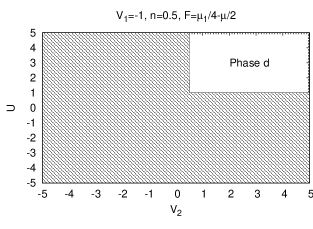
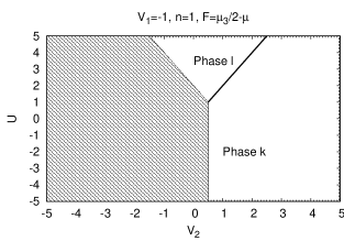
Figure 4: Phase diagram in the case $V_{1}=-1$ for $n=0.5$ and $n=1$. In the shaded areas the jump in the dependence $\mu(n)$ is absent at the given commensurate $n$.

III.2 Case $V_{1}=-1$

Let us consider now the phase diagram in the case $V_{1}=-1$. The differences with respect to the case $V_{1}=1$ emerge when one starts to consider the existence conditions for the commensurate phases at $n=\frac{1}{4}$ ($n=\frac{3}{4}$) and $n=\frac{1}{2}$. The former is equivalent to $\mu_{1}>0$ and one can easily verify that in our case it is never satisfied, which means that there are no jumps at $n=\frac{1}{4}$ and $\frac{3}{4}$ in $\mu(n)$ and the phases at those precise $n$ do not exist. For the existence of the phase at $n=\frac{1}{2}$ it is necessary (and sufficient) that $\mu_{1}<\mu_{3}$. By inspection, one can verify that the range of existence of any phase at $n=\frac{1}{2}$ is $V_{2}>\frac{1}{2}\land U>1$. Moreover, at $V_{1}=-1$, the jump at $n=1$ will exist only in the range $V_{2}>\frac{1}{2}$ and $U>1$, i.e. in the same range where the jump at $n=\frac{1}{2}$ exists. In Fig. 4 we report the phases at $n=\frac{1}{2}$ and $n=1$. Only the Phases $d$, $l$ and $k$ are present at $V_{1}=-1$ and their description has been given above.

Figure 5: Phase diagram in the case $V_{1}=-1$ and for arbitrary $n$.

The incommensurate phase diagram, shown in Fig. 5, splits into two cases: $n<\frac{1}{2}$ and $n>\frac{1}{2}$. In addition, only in this case there appears the Phase 8, in which all the fundamental CFs are different from zero.

III.2.1 $0<n<\frac{1}{2}$

Several phases are present in this case. The Phase 3, characterized by only NN correlations, extends in the domains: $2V_{2}>-V_{1}$, $U>-V_{1}$; the Phase 4 is placed in the range $2V_{2}<-V_{1}$, $U>-2V_{1}-2V_{2}$. The Phase 7 exists in the range $2V_{2}>-V_{1}$, $U<-V_{1}$, while the Phase 8 occupies the area $\max\left(2V_{2},2V_{1}-2V_{2}\right)<U<-2V_{1}-2V_{2}$.

III.2.2 $\frac{1}{2}<n<1$

At fillings larger than $\frac{1}{2}$, a little changes in the phase diagram: the range $2V_{2}>-V_{1}$, $U>-V_{1}$, previously dominated by the Phase 3, is now occupied by the Phases 4 and 7. These latter enlarge and fill in the following areas: Phase 4 $U>\max\{2V_{2},-2V_{1}-2V_{2}\}$, Phase 7 $U<2V_{2}$, $-V_{1}<2V_{2}$.

IV Thermodynamic properties

We have shown in the previous Section that at zero temperature it is always possible to determine analytically all the properties of the system at any point in the phase diagram of the Hamiltonian (2). At finite $T$, the whole spectrum is involved and the appearance of various features in the thermodynamic quantities (TQs) depends on the exact positions and degeneracies of all energy levels in the system. Therefore, we adopt the following scheme to analyze the low-$T$ properties of TQs: we estimate the level of the charge rigidity of the ground state, the gaps between the ground state and few low-lying excited states and the ratio of degeneracy of these excited states with respect to the ground state degeneracy, when these excited states are well separated from the rest of the spectrum. Finally, we study the behavior of the aforementioned TQs across the $T=0$ phase boundaries and follow the change of the properties upon switching on the temperature. Following this scheme, we have studied the behaviors of the TQs in various phases and across various phase boundaries, and report below the most representative ones. We note that the TQs change not only at the boundaries of the macro-phases but also crossing the different phases inside the same macro-phase.

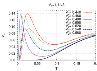
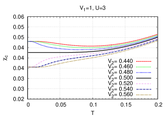
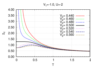
Figure 6: (Color online) Left panel: the behavior of the specific heat $c_{n}(T)$ across the phase boundary in a typical $T=0$ phase transition. $n=0.4$, $V_{1}=1$, $U=3$, the transition occurs at $V_{2}=0.5$. Middle and right panels: the behavior of the charge susceptibility $\chi_{c}(T)$ across the phase boundaries in two representative cases. Middle panel: $n=0.4$, $V_{1}=1$, $U=3$, the transition occurs at $V_{2}=0.5$; right panel: $n=0.4$, $V_{1}=-1$, $U=-2$, the transition occurs at $V_{2}=0.5$.

In the present Section, we focus on the following TQs: specific heat, charge susceptibility and entropy. The specific heat at constant $n$ is defined as follows:

$$c_{n}=\left(\frac{\partial E}{\partial T}\right)_{n},$$ (22)

where $E$ is the internal energy. The specific heat of the model under investigation presents in general a multiple-peak structure and goes to zero in the limits $T\to 0$ and $T\to\infty$.

We define the charge susceptibility as follows:

$$\chi_{c}=T\frac{\partial n}{\partial\mu}.$$ (23)

$\chi_{c}$ in the model (2) can either diverge, go to zero, or go to a finite limit as $T\to 0$. A divergent susceptibility signifies the rigidity of the underlying configuration with respect to the addition of electrons.

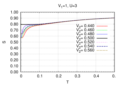
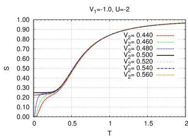
Figure 7: (Color online) The behavior of the entropy $S(T)$ across the phase boundaries in two representative cases. Upper panel: $n=0.4$, $V_{1}=1$, $U=3$, the transition occurs at $V_{2}=0.5$; Lower panel: $n=0.4$, $V_{1}=-1$, $U=-2$, the transition occurs at $V_{2}=0.5$.

The entropy is defined as the partial derivative of the free energy with respect to the temperature and, as such, can be easily computed within the Transfer Matrix method. One usually is interested in the $T\to 0$ limit of entropy since it indicates, if non-zero, a ground-state degeneracy.

In the low-temperature limit, the properties of the system are determined, to a great extent, by the properties of the ground state and of a few excited ones. When only the first excited state is involved, the system resembles a two-level one. We will show in the following that several features of the two-level system are present in TQs of (2) at low temperatures. In order to do that, we summarize below the results for a generic two-level system. Suppose that we have a system with two levels $0$ and $\Delta$. Each level can be degenerate with its own degeneracy $N_{0}$ and $N_{1}$, respectively. It can be easily checked that in such a toy system $c_{n}$, $S$ and the internal energy $E$ can be expressed as follows:

$$\begin{split}c_{n}&=\left(\frac{\Delta}{T}\right)^{2}\frac{e^{\frac{\Delta}{T}+A}}{\left(1+e^{\frac{\Delta}{T}+A}\right)^{2}}\\ S&=\log N_{0}+\log\left(1+e^{-\frac{\Delta}{T}-A}\right)+\frac{E}{T}\\ E&=\frac{\Delta}{1+e^{\frac{\Delta}{T}+A}},\end{split}$$ (24)

where $A=\log\frac{N_{0}}{N_{1}}$. At fixed $A$, the position of the maximum of $c_{n}$ depends linearly on $\Delta$: $T^{\star}=\frac{\Delta}{2\xi}$, where $\xi$ is the solution of the transcendental equation:

$$\xi=\coth\left(\xi+\frac{A}{2}\right),$$ (25)

while the height of the maximum appears to be independent of $\Delta$. The limit of entropy at $T\to 0$ is equal to $\log N_{0}$ and, thus, is non-zero for degenerate ground states. After a careful analysis of the whole phase diagram of the model we have identified the typical behaviors of each TQs across the phase boundaries.

Specific heat: The low-$T$ behavior of the specific heat $c_{n}$ across the $T=0$ phase transitions is common to the whole phase diagram. A representative of such behavior is shown in Fig. 6. $c_{n}$ develops a low-$T$ peak, whose position approaches gradually zero as the system reaches the transition (in case of Fig. 6 at $V_{2}=0.5$), while the height of the peak remains constant. On the opposite side of the transition, the picture is analogous except for the difference in the peak height.

The appearance of such a low-$T$ peak can be associated to the first excited state. Indeed, as in the two-level system, the height of the low-$T$ peak does not depend on the vicinity to the transition $\zeta$, while the peak position depends linearly on $\zeta$, as can be seen from Fig. 6. Here we define $\zeta$ as the shortest distance from a given point in the phase diagram to the transition line. The study of the first excited state not only sheds light on the low-$T$ behavior of TQs. It appears from our analysis that the transitions among various $T=0$ phases take place via the exchange of the ground state with the first excited one. In the case of Fig. 6, the transition occurs at $V_{2}=\frac{1}{2}$; the ground state energy at $V_{2}<\frac{1}{2}$ is $2V_{2}\left(n-\frac{1}{4}\right)$, the ground state energy at $V_{2}>\frac{1}{2}$ is $V_{1}\left(n-\frac{1}{4}\right)$, and thus $\Delta=|V_{1}-2V_{2}|\left(n-\frac{1}{4}\right)$. During this transition $V_{1}=1$ and the path across the transition passes along the line $U=3$. $\Delta$ decreases linearly as $V_{2}$ approaches $\frac{1}{2}$ and so should also do the low-$T$ peak in $c_{n}$, which is indeed the case, as shown in Fig. 6.

Charge susceptibility and entropy: Unlikely the specific heat, charge susceptibility and entropy exhibit several distinct behaviors: the divergence of $\chi_{c}$ at $T\to 0$ is accompanied by a vanishing entropy, while finite $\chi_{c}$ at $T\to 0$ corresponds to a finite entropy in the same limit. Examples of such behaviours are shown Fig. 7. The divergence of the charge susceptibility indicates the rigidity of the ground state configuration with respect to addition of electrons, while a finite entropy at $T\to 0$ indicates a ground state degeneracy.

V Concluding remarks

In the present manuscript, we apply the Transfer Matrix method to find the exact solution for the atomic limit of the 1D Hubbard model supplied with NN and NNN density-density correlations terms. We utilize the TM technique in order to fulfil a thorough analysis of both $T=0$ and finite-temperature properties of the model under consideration. Several competing interactions induce a quite large number of $T=0$ phases, and the use of the TM technique allows us to completely catalogue their properties, including the exact analytic forms for the internal energy and fundamental correlation functions. The study of the thermodynamic quantities reveals a few peculiarities of the system under consideration: a considerable amount of the phases has a macroscopic degeneracy, manifested by a finite entropy in the limit $T\to 0$; this is due to the fact that the Hamiltonian acts only in the charge density sector leaving the degeneracy with respect to the spin configurations. On the other hand, even in the charge density sector, a few phases exhibit a finite entropy at $T\to 0$, owing to the phase separated states inherent to the atomic models. Some of these states have been already found in literature in various limiting cases of our model robaszkiewicz_00 ; mancini_33 ; Bursill_00 . Physically, such phases are composed of a superposition of a huge amount of electronic configurations, each made of blocks of filled sites separated by blocks of empty ones. Such a block structure gives origin to a large degeneracy, which often survives in the thermodynamic limit. Moreover, by studying the low temperature features of the specific heat, we find that transitions among various phases occur through the exchange between the first excited and the ground states.

From the viewpoint of methodology, we present a number of useful extensions to the standard TM technique: symmetrization of the TM, rank reduction of the TM by use of the system’s symmetries, obtaining the ground state phase diagram from the TM matrix elements and conversion of the grand canonical phase diagram to the canonical one. Finally, we show how the properties of the first excited state of the model can be inferred from the low-temperature behavior of the thermodynamic quantities such as the specific heat, charge susceptibility and entropy.

The study of an easily solvable model such as the one considered here, can be considered as a starting point for the analysis of more involved models. In particular, we identify two lines, along which the work is currently in progress: i) extention of the treatment to an $n$-leg ladder and successively to a 2D square lattice mancini_10 ; ii) introduction of the kinetic energy in order to treat it as a small perturbation. Plenty of new physical effects should arise upon switching on of the kinetic energy. In particular, taking into account the extended Coulomb interactions ($V_{1}$ and $V_{2}$), it would be extremely interesting to study the Mott insulating phases at the commensurate fillings $n_{comm}$. In addition, we expect the spin channel of the model to become active in this case.

Appendix A Explicit form of the TM

For the sake of completeness, we report here the explicit form of the TM for the model (2). Here the quantities $F_{n}^{i}$ denote the exponentiated energy scales from Table 2 ($E^{i}_{n}$) according to the following definition:

$$F^{i}_{n}=\exp\left(-\frac{E_{n}^{i}}{T}\right),$$ (26)

where the lower index $n$ denotes one of the commensurate fillings $n_{comm}$. If several energy scales correspond to a given $n$, these are labeled by the upper index $i$ corresponding to the order in which the energy scales appear in Table 2.

$$Z(1,2)=\left(\begin{array}[]{cccccccccccccccc}1&F_{\frac{1}{4}}&F_{\frac{1}{4}}&F_{\frac{1}{2}}^{2}&F_{\frac{1}{4}}&F_{\frac{1}{2}}^{3}&F_{\frac{1}{2}}^{3}&F_{\frac{3}{4}}^{2}&F_{\frac{1}{4}}&F_{\frac{1}{2}}^{3}&F_{\frac{1}{2}}^{3}&F_{\frac{3}{4}}^{2}&F_{\frac{1}{2}}^{2}&F_{\frac{3}{4}}^{2}&F_{\frac{3}{4}}^{2}&F_{1}^{2}\\ F_{\frac{1}{4}}&F_{\frac{1}{2}}^{1}&F_{\frac{1}{2}}^{1}&F_{\frac{3}{4}}^{1}&F_{\frac{1}{2}}^{3}&F_{\frac{3}{4}}^{3}&F_{\frac{3}{4}}^{3}&F_{1}^{3}&F_{\frac{1}{2}}^{3}&F_{\frac{3}{4}}^{3}&F_{\frac{3}{4}}^{3}&F_{1}^{3}&F_{\frac{3}{4}}^{2}&F_{1}^{4}&F_{1}^{4}&F_{\frac{5}{4}}^{2}\\ F_{\frac{1}{4}}&F_{\frac{1}{2}}^{1}&F_{\frac{1}{2}}^{1}&F_{\frac{3}{4}}^{1}&F_{\frac{1}{2}}^{3}&F_{\frac{3}{4}}^{3}&F_{\frac{3}{4}}^{3}&F_{1}^{3}&F_{\frac{1}{2}}^{3}&F_{\frac{3}{4}}^{3}&F_{\frac{3}{4}}^{3}&F_{1}^{3}&F_{\frac{3}{4}}^{2}&F_{1}^{4}&F_{1}^{4}&F_{\frac{5}{4}}^{2}\\ F_{\frac{1}{2}}^{2}&F_{\frac{3}{4}}^{1}&F_{\frac{3}{4}}^{1}&F_{1}^{1}&F_{\frac{3}{4}}^{2}&F_{1}^{3}&F_{1}^{3}&F_{\frac{5}{4}}^{1}&F_{\frac{3}{4}}^{2}&F_{1}^{3}&F_{1}^{3}&F_{\frac{5}{4}}^{1}&F_{1}^{2}&F_{\frac{5}{4}}^{2}&F_{\frac{5}{4}}^{2}&F_{\frac{3}{2}}^{2}\\ F_{\frac{1}{4}}&F_{\frac{1}{2}}^{3}&F_{\frac{1}{2}}^{3}&F_{\frac{3}{4}}^{2}&F_{\frac{1}{2}}^{1}&F_{\frac{3}{4}}^{3}&F_{\frac{3}{4}}^{3}&F_{1}^{4}&F_{\frac{1}{2}}^{1}&F_{\frac{3}{4}}^{3}&F_{\frac{3}{4}}^{3}&F_{1}^{4}&F_{\frac{3}{4}}^{1}&F_{1}^{3}&F_{1}^{3}&F_{\frac{5}{4}}^{2}\\ F_{\frac{1}{2}}^{3}&F_{\frac{3}{4}}^{3}&F_{\frac{3}{4}}^{3}&F_{1}^{3}&F_{\frac{3}{4}}^{3}&F_{1}^{5}&F_{1}^{5}&F_{\frac{5}{4}}^{3}&F_{\frac{3}{4}}^{3}&F_{1}^{5}&F_{1}^{5}&F_{\frac{5}{4}}^{3}&F_{1}^{3}&F_{\frac{5}{4}}^{3}&F_{\frac{5}{4}}^{3}&F_{\frac{3}{2}}^{3}\\ F_{\frac{1}{2}}^{3}&F_{\frac{3}{4}}^{3}&F_{\frac{3}{4}}^{3}&F_{1}^{3}&F_{\frac{3}{4}}^{3}&F_{1}^{5}&F_{1}^{5}&F_{\frac{5}{4}}^{3}&F_{\frac{3}{4}}^{3}&F_{1}^{5}&F_{1}^{5}&F_{\frac{5}{4}}^{3}&F_{1}^{3}&F_{\frac{5}{4}}^{3}&F_{\frac{5}{4}}^{3}&F_{\frac{3}{2}}^{3}\\ F_{\frac{3}{4}}^{2}&F_{1}^{3}&F_{1}^{3}&F_{\frac{5}{4}}^{1}&F_{1}^{4}&F_{\frac{5}{4}}^{3}&F_{\frac{5}{4}}^{3}&F_{\frac{3}{2}}^{1}&F_{1}^{4}&F_{\frac{5}{4}}^{3}&F_{\frac{5}{4}}^{3}&F_{\frac{3}{2}}^{1}&F_{\frac{5}{4}}^{2}&F_{\frac{3}{2}}^{3}&F_{\frac{3}{2}}^{3}&F_{\frac{7}{4}}\\ F_{\frac{1}{4}}&F_{\frac{1}{2}}^{3}&F_{\frac{1}{2}}^{3}&F_{\frac{3}{4}}^{2}&F_{\frac{1}{2}}^{1}&F_{\frac{3}{4}}^{3}&F_{\frac{3}{4}}^{3}&F_{1}^{4}&F_{\frac{1}{2}}^{1}&F_{\frac{3}{4}}^{3}&F_{\frac{3}{4}}^{3}&F_{1}^{4}&F_{\frac{3}{4}}^{1}&F_{1}^{3}&F_{1}^{3}&F_{\frac{5}{4}}^{2}\\ F_{\frac{1}{2}}^{3}&F_{\frac{3}{4}}^{3}&F_{\frac{3}{4}}^{3}&F_{1}^{3}&F_{\frac{3}{4}}^{3}&F_{1}^{5}&F_{1}^{5}&F_{\frac{5}{4}}^{3}&F_{\frac{3}{4}}^{3}&F_{1}^{5}&F_{1}^{5}&F_{\frac{5}{4}}^{3}&F_{1}^{3}&F_{\frac{5}{4}}^{3}&F_{\frac{5}{4}}^{3}&F_{\frac{3}{2}}^{3}\\ F_{\frac{1}{2}}^{3}&F_{\frac{3}{4}}^{3}&F_{\frac{3}{4}}^{3}&F_{1}^{3}&F_{\frac{3}{4}}^{3}&F_{1}^{5}&F_{1}^{5}&F_{\frac{5}{4}}^{3}&F_{\frac{3}{4}}^{3}&F_{1}^{5}&F_{1}^{5}&F_{\frac{5}{4}}^{3}&F_{1}^{3}&F_{\frac{5}{4}}^{3}&F_{\frac{5}{4}}^{3}&F_{\frac{3}{2}}^{3}\\ F_{\frac{3}{4}}^{2}&F_{1}^{3}&F_{1}^{3}&F_{\frac{5}{4}}^{1}&F_{1}^{4}&F_{\frac{5}{4}}^{3}&F_{\frac{5}{4}}^{3}&F_{\frac{3}{2}}^{1}&F_{1}^{4}&F_{\frac{5}{4}}^{3}&F_{\frac{5}{4}}^{3}&F_{\frac{3}{2}}^{1}&F_{\frac{5}{4}}^{2}&F_{\frac{3}{2}}^{3}&F_{\frac{3}{2}}^{3}&F_{\frac{7}{4}}\\ F_{\frac{1}{2}}^{2}&F_{\frac{3}{4}}^{2}&F_{\frac{3}{4}}^{2}&F_{1}^{2}&F_{\frac{3}{4}}^{1}&F_{1}^{3}&F_{1}^{3}&F_{\frac{5}{4}}^{2}&F_{\frac{3}{4}}^{1}&F_{1}^{3}&F_{1}^{3}&F_{\frac{5}{4}}^{2}&F_{1}^{1}&F_{\frac{5}{4}}^{1}&F_{\frac{5}{4}}^{1}&F_{\frac{3}{2}}^{2}\\ F_{\frac{3}{4}}^{2}&F_{1}^{4}&F_{1}^{4}&F_{\frac{5}{4}}^{2}&F_{1}^{3}&F_{\frac{5}{4}}^{3}&F_{\frac{5}{4}}^{3}&F_{\frac{3}{2}}^{3}&F_{1}^{3}&F_{\frac{5}{4}}^{3}&F_{\frac{5}{4}}^{3}&F_{\frac{3}{2}}^{3}&F_{\frac{5}{4}}^{1}&F_{\frac{3}{2}}^{1}&F_{\frac{3}{2}}^{1}&F_{\frac{7}{4}}\\ F_{\frac{3}{4}}^{2}&F_{1}^{4}&F_{1}^{4}&F_{\frac{5}{4}}^{2}&F_{1}^{3}&F_{\frac{5}{4}}^{3}&F_{\frac{5}{4}}^{3}&F_{\frac{3}{2}}^{3}&F_{1}^{3}&F_{\frac{5}{4}}^{3}&F_{\frac{5}{4}}^{3}&F_{\frac{3}{2}}^{3}&F_{\frac{5}{4}}^{1}&F_{\frac{3}{2}}^{1}&F_{\frac{3}{2}}^{1}&F_{\frac{7}{4}}\\ F_{1}^{2}&F_{\frac{5}{4}}^{2}&F_{\frac{5}{4}}^{2}&F_{\frac{3}{2}}^{2}&F_{\frac{5}{4}}^{2}&F_{\frac{3}{2}}^{3}&F_{\frac{3}{2}}^{3}&F_{\frac{7}{4}}&F_{\frac{5}{4}}^{2}&F_{\frac{3}{2}}^{3}&F_{\frac{3}{2}}^{3}&F_{\frac{7}{4}}&F_{\frac{3}{2}}^{2}&F_{\frac{7}{4}}&F_{\frac{7}{4}}&F_{2}\\ \end{array}\right).$$ (27)

Table 3: The complete list of the phases of the model (2), their existence ranges and ground-state energies.

Phase	Existence range $V_{2}$, $U$	Existence range $n$	Energy per site
$V_{1}=+1$
I	$U>0\land V_{2}>0$	$0<n<\frac{1}{4}$	$0$
II	$U<-2V_{2}\land V_{2}<0$	$0<n<1$	$U\frac{n}{2}+2V_{2}n$
III	$U>-2V_{2}\land V_{2}<0$	$0<n<\frac{1}{2}$	$V_{2}n$
IV	$U<0\land V_{2}>0$	$0<n<\frac{1}{2}$	$\frac{Un}{2}$
V	$U>2V_{2}\land 0<V_{2}<\frac{1}{2}$	$\frac{1}{4}<n<\frac{1}{2}$	$2V_{2}\left(n-\frac{1}{4}\right)$
VI	$U>1\land V_{2}>\frac{1}{2}$	$\frac{1}{4}<n<\frac{1}{2}$	$V_{1}\left(n-\frac{1}{4}\right)$
VII	$0<U<1\land 2V_{2}>U$	$\frac{1}{4}<n<\frac{1}{2}$	$U\left(n-\frac{1}{4}\right)$
VIII	$-2V_{2}<U<2-2V_{2}\land V_{2}<0$	$\frac{1}{2}<n<1$	$U\left(n-\frac{1}{2}\right)+V_{2}(3n-1)$
IX	$U>2-2V_{2}\land V_{2}<0$	$\frac{1}{2}<n<1$	$V_{1}\left(2n-1\right)+V_{2}n$
X	$U>-2V_{2}\land 0<V_{2}<\frac{1}{2}$	$\frac{1}{2}<n<\frac{3}{4}$	$V_{1}\left(2n-1\right)+\frac{V_{2}}{2}$
XI	$U>2V_{2}\land V_{2}>\frac{1}{2}$	$\frac{1}{2}<n<\frac{3}{4}$	$V_{2}\left(2n-1\right)+V_{1}\left(n-\frac{1}{4}\right)$
XII	$1<U<2V_{2}$	$\frac{1}{2}<n<\frac{3}{4}$	$U\left(n-\frac{1}{2}\right)+V_{1}\left(n-\frac{1}{4}\right)$
XIII	$2V_{2}<U<2-2V_{2}\land 0<V_{2}<\frac{1}{2}$	$\frac{1}{2}<n<\frac{3}{4}$	$U\left(n-\frac{1}{2}\right)+2V_{2}\left(n-\frac{1}{4}\right)$
XIV	$0<U<2V_{2}\land 0<V_{2}<\frac{1}{2}$	$\frac{1}{2}<n<\frac{3}{4}$	$2V_{2}\left(2n-1\right)+\frac{U}{4}$
XV	$0<U<1\land V_{2}>\frac{1}{2}$	$\frac{1}{2}<n<\frac{3}{4}$	$V_{1}\left(2n-1\right)+\frac{U}{4}$
XVI	$U<0\land V_{2}>\frac{1}{2}$	$\frac{1}{2}<n<1$	$V_{1}\left(2n-1\right)+\frac{Un}{2}$
XVII	$U<0\land 0<V_{2}<\frac{1}{2}$	$\frac{1}{2}<n<1$	$2V_{2}\left(2n-1\right)+\frac{Un}{2}$
XVIII	$U>\max\{2V_{2},2-2V_{2}\}\land V_{2}>0$	$\frac{3}{4}<n<1$	$2(V_{1}+V_{2})\left(n-\frac{1}{2}\right)$
XIX	$U<2V_{2}\land V_{2}>\frac{1}{2}$	$\frac{3}{4}<n<1$	$(U+2V_{1})\left(n-\frac{1}{2}\right)$
XX	$0<U<2-2V_{2}\land 0<V_{2}<\frac{1}{2}$	$\frac{3}{4}<n<1$	$(U+4V_{2})\left(n-\frac{1}{2}\right)$
$V_{1}=-1$
XXI	$U<2-2V_{2}\land V_{2}<\frac{1}{2}$	$0<n<2$	$(U+4V_{1}+4V_{2})\frac{n}{2}$
XXII	$U>2-2V_{2}\land V_{2}<\frac{1}{2}$	$0<n<1$	$(V_{1}+V_{2})n$
XXIII	$U<1\land V_{2}>\frac{1}{2}$	$0<n<1$	$\left(\frac{U}{2}+V_{1}\right)n$
XXIV	$U>1\land V_{2}>\frac{1}{2}$	$0<n<\frac{1}{2}$	$\frac{V_{1}n}{2}$
XXV	$U>2V_{2}\land V_{2}>\frac{1}{2}$	$\frac{1}{2}<n<1$	$\frac{V_{1}}{2}\left(3n-1\right)+2V_{2}(n-\frac{1}{2})$
XXVI	$1<U<2V_{2}\land V_{2}>\frac{1}{2}$	$\frac{1}{2}<n<1$	$\frac{V_{1}}{2}\left(3n-1\right)+U(n-\frac{1}{2})$

Appendix B Micro-phases

In Table 3, we present all the micro-phases of the model under investigation and summarize their properties. Namely, for each micro-phase we report the existence ranges both in terms of $U,V_{1},V_{2}$ and in terms of $n$ as well as the exact expression for the ground state energy, which can be used to extract the fundamental correlation functions.

References

- (1) J. Hubbard, Proc. R. Soc. Lond. A 276, 238 (1963)
- (2) S. Miyashita, Prog. Theor. Phys. 120, 785 (2008)
- (3) H. Tasaki, Eur. Phys. J. B 64, 365 (2008)
- (4) M. Fleck, A. I. Lichtenstein, E. Pavarini, and A. M. Oleś, Phys. Rev. Lett. 84, 4962 (2000)
- (5) H. Schweitzer and G. Czycholl, Z. Phys. B 83, 93 (1991), ISSN 0722
- (6) S. Pankov and V. Dobrosavljević, Phys. Rev. B 77, 085104 (2008)
- (7) P. W. Anderson, Science 235, 1196 (1987)
- (8) R. Micnas, J. Ranninger, S. Robaszkiewicz, and S. Tabor, Phys. Rev. B 37, 9410 (1988)
- (9) E. Dagotto, T. Hotta, and A. Moreo, Phys. Rep. 344, 1 (2001)
- (10) C. N. R. Rao, A. Arulraj, A. K. Cheetham, and B. Raveau, J. Phys: Cond. Mat. 12, R83 (2000)
- (11) B. Muschler, W. Prestel, L. Tassini, R. Hackl, M. Lambacher, A. Erb, S. Komiya, Y. Ando, D. C. Peets, W. N. Hardy, R. Liang, and D. A. Bonn, Eur. Phys. J-Spec. Top. 188, 131 (2010)
- (12) T. Mori, M. Katsuhara, S. Kimura, Y. Misaki, and K. Tanaka, Synth. Met. 133-134, 281 (2003)
- (13) H. Seo, J. Phys. Soc. Jpn. 69, 805 (2000)
- (14) H. Yoshioka, M. Tsuchiizu, and Y. Suzumura, J. Phys. Soc. Jpn. 70, 762 (2001)
- (15) H. Bethe, Z. Phys. 71, 205 (1931)
- (16) G. Esirgen, H.-B. Schüttler, and N. E. Bickers, Phys. Rev. Lett. 82, 1217 (1999)
- (17) Y. Tomio, N. Dupuis, and Y. Suzumura, Phys. Rev. B 64, 125123 (2001)
- (18) M. Murakami, J. Phys. Soc. Jpn. 69, 1113 (2000)
- (19) W. P. Su, Phys. Rev. B 69, 012506 (2004)
- (20) W. P. Su and Y. Chen, Phys. Rev. B 64, 172507 (2001)
- (21) M. Onozawa, Y. Fukumoto, A. Oguchi, and Y. Mizuno, Phys. Rev. B 62, 9648 (2000)
- (22) M. Tsuchiizu and A. Furusaki, Phys. Rev. Lett. 88, 056402 (2002)
- (23) M. Nakamura, J. Phys. Soc. Jpn. 68, 3123 (1999)
- (24) G. Japaridze and S. Sarkar, Eur. Phys. J. B 28, 139 (2002), ISSN 1434-6028
- (25) E. Plekhanov, S. Sorella, and M. Fabrizio, Phys. Rev. Lett. 90, 187004 (2003)
- (26) T. Giamarchi, Quantum Physics in One Dimension (Oxford University Press, 2004) ISBN 0198525001
- (27) A. Avella and F. Mancini, Eur. Phys. J. B 41, 149 (2004)
- (28) M. Nakamura, A. Kitazawa, and K. Nomura, Phys. Rev. B 60, 7850 (1999)
- (29) P. Sengupta, A. W. Sandvik, and D. K. Campbell, Phys. Rev. B 65, 155113 (2002)
- (30) A. W. Sandvik, L. Balents, and D. K. Campbell, Phys. Rev. Lett. 92, 236401 (2004)
- (31) S. Ejima and S. Nishimoto, Phys. Rev. Lett. 99, 216403 (2007)
- (32) S. Glocke, A. Klümper, and J. Sirker, Phys. Rev. B 76, 155121 (2007)
- (33) A. Avella and F. Mancini, J. Phys. Chem. Solids 67, 142 (2006)
- (34) A. Avella, F. Mancini, D. Villani, and H. Matsumoto, Eur. Phys. J. B 20, 303 (2001)
- (35) A. Avella and F. Mancini, Physica C 408, 284 (2004)
- (36) J. Jędrzejewski, Z. Phys. B 59, 325 (1985)
- (37) J. Jędrzejewski, Physica A 205, 702 (1994)
- (38) K. Kapcia and S. Robaszkiewicz, Journal of Physics: Condensed Matter 23, 105601 (2011)
- (39) R. J. Baxter, Exactly Solved Models in Statistical Mechanics (Dover Publications, 2007) ISBN 0486462714
- (40) R. A. Bari, Phys. Rev. B 3, 2662 (1971)
- (41) G. Beni and P. Pincus, Phys. Rev. B 9, 2963 (1974)
- (42) R. S. Tu and T. A. Kaplan, Phys. Stat. Sol. B 63, 659 (1974)
- (43) F. Mancini and F. Mancini, Phys. Rev. E 77, 061120 (2008), http://dx.doi.org/10.1103/PhysRevE.77.061120
- (44) F. Mancini and F. P. Mancini, Eur. Phys. J. B 73, 581 (2010)
- (45) K. Kapcia, W. Klobus, and S. Robaszkiewicz, Acta Phys. Pol. A 118, 353 (2010)
- (46) K. Kapcia and S. Robaszkiewicz, Acta Phys. Pol. A 121, 1029 (2012)
- (47) M. Blume, V. J. Emery, and R. B. Griffiths, Phys. Rev. A 4, 1071 (1971)
- (48) F. Mancini and F. P. Mancini, Cond. Mat. Phys. 11, 543 (2008)
- (49) R. J. Bursill and C. J. Thompson, Journal of Physics A: Mathematical and General 26, 4497 (1993)
- (50) F. Mancini, AIP Conference Proceedings 1198, 95 (2009)