Remapping dark matter halo catalogues between cosmological simulations

Abstract

We present and test a method for modifying the catalogue of dark matter haloes produced from a given cosmological simulation, so that it resembles the result of a simulation with an entirely different set of parameters. This extends the method of Angulo & White (2010), which rescales the full particle distribution from a simulation. Working directly with the halo catalogue offers an advantage in speed, and also allows modifications of the internal structure of the haloes to account for nonlinear differences between cosmologies. Our method can be used directly on a halo catalogue in a self contained manner without any additional information about the overall density field; although the large-scale displacement field is required by the method, this can be inferred from the halo catalogue alone. We show proof of concept of our method by rescaling a matter-only simulation with no baryon acoustic oscillation (BAO) features to a more standard $\Lambda$CDM model containing a cosmological constant and a BAO signal. In conjunction with the halo occupation approach, this method provides a basis for the rapid generation of mock galaxy samples spanning a wide range of cosmological parameters.

1 Introduction

Ever since the first measurements of the accelerated expansion of the cosmos from supernova data (Schmidt et al. 1998; Perlmutter et al. 1999), the origin of the acceleration has been a dominant, open question in cosmology. Either space is filled with a nearly homogeneous substance, dark energy, or we are witnessing a breakdown of Einstein’s relativistic gravity on cosmological scales. Exploring these issues, and looking for deviations from a pure cosmological constant, requires us to measure the global expansion history precisely, together with the rate of growth of density fluctuations. The expansion history involves standard candles and standard rulers, especially the signal of BAO (Baryon Acoustic Oscillations) in the galaxy distribution (e.g. Anderson et al. 2013); the growth rate can be probed directly by gravitational lensing (e.g. CFHTLens: Heymans et al. 2012) or via redshift-space distortions in galaxy clustering (e.g. Samushia et al. 2013; de la Torre et al. 2013).

The extraction of this fundamental cosmological information increasingly requires a major input from cosmological $N$-body simulations, for two reasons. The statistical quantities to be measured from the data tend to have complicated correlations, and the only practical way of computing the required covariance matrix is by averaging over an ensemble of mock datasets. More seriously, an analytical understanding of the development of cosmological structure is restricted to large-scale linear fluctuations, whereas the measurements are inevitably affected by small-scale nonlinearities to some extent. The mildly nonlinear regime can be explored with perturbation theory (e.g. Bernardeau et al. 2002) but this fails on smaller scales. If nonlinear information is to be exploited, it is necessary to run simulations for different sets of cosmological parameters, to measure the matter distribution and derive halo catalogues. Mock galaxy samples can then either be generated using semi-analytic methods (e.g. Baugh 2006) or from halo occupation distribution models (Seljak 2000; Peacock & Smith 2000; Zheng et al. 2005).

However, it is computationally prohibitive to run simulations of large enough volumes at a high enough resolution in order to cover the current cosmological parameter space, which has now grown to encompass neutrinos (masses and numbers of species); warm dark matter; plus complex dark energy models and modified gravity theories. We therefore need some way of spanning this range of cosmologies without having to run a simulation for each particular set of parameters. This idea was investigated by Angulo & White (2010; hereafter AW10), who showed that it was possible to rescale an $N$-body particle distribution in order to approximate the results of a simulation with a different set of cosmological parameters. Their algorithm consisted of two steps: (i) reinterpreting the length and time units in the original simulation so that the halo mass function was as close as possible to that which would be measured in the new cosmology (ii) modifying individual particle positions so as to reproduce the expected linear clustering in the new cosmology.

AW10 showed that their method successfully reproduced the statistics of the target cosmology at the level of the matter power spectrum and halo mass function. AW10 has been applied by Guo et al. (2013) to look at theoretical differences in galaxy formation between WMAP1 and WMAP7 cosmologies and by Simha & Cole (2013), who looked at measuring cosmological parameters by comparing the galaxy two-point correlation function of SDSS with that computed from galaxy catalogues that were rescaled using the AW10 method.

Despite the success of the AW10 algorithm, it has some disadvantages. Firstly, the algorithm is applied to large particle datasets that can be difficult to communicate; often it is only halo catalogues that are made publicly available by large collaborative simulation groups (e.g. the DEUSS simulations of Rasera et al. 2010). Secondly, the algorithm uses the displacement field that was employed to generate the initial conditions; again this may not be publicly available. Finally, the algorithm reproduces the linear clustering in the target simulation, but does not reproduce the deeply nonlinear clustering, which can be considered to be associated with correlations within individual haloes. In this paper we develop and test an extension to the AW10 algorithm designed to deal with these issues.

Our method rapidly converts a halo catalogue from a given simulation into one that is characteristic of a different cosmology. Other methods for the fast generation of halo catalogues have been developed in the literature: Monaco et al. (2002) developed an algorithm called PINOCCHIO, which uses a combination of perturbation theory and an ellipsoidal halo collapse model to generate catalogues. Manera et al. (2013) produced mock catalogues for the Baryon Oscillation Spectroscopic Survey (BOSS) using second order Lagrangian perturbation theory (2LPT) on a particle distribution and then collecting mass from the evolved field into haloes; this approach is called PTHaloes. Tassev et al. (2013) use an approach called COLA (COmoving Lagrangian Acceleration), which involves a coordinate transform based on 2LPT, followed by a particle mesh (PM) gravity solver with coarse time-stepping, which is able to yield halo statistics rapidly. Nevertheless, all these methods are approximate in their treatment of nonlinearities, and an attractive feature of AW10 is that it is based on a fully nonlinear simulation. A reduced version of the AW10 method has been applied to halo catalogues by Ruiz et al. (2011), in which the authors scaled a halo catalogue in time and length units but did not apply the final stage of the algorithm, in which the linear clustering is reproduced by modifying individual halo positions. In this case Ruiz et al. (2011) showed that AW10 works very well on halo catalogues, but only for simulations of small box sizes ($<50\,h^{-1}\,\mathrm{Mpc}$) in which large-scale shifts in the displacement field are unimportant and would only manifest themselves as translations of the entire box. Nevertheless the authors showed that halo positions and velocities were recovered with almost no detectable biases and information useful for galaxy formation modelling, such as merger histories, could also be accurately recovered.

Our extended algorithm consists of the following steps: The length and time units in the original halo catalogue are rescaled exactly as in the original AW10 algorithm. We then use the particles or halo distribution itself to compute the linear displacement field, from which we modify the particle or halo positions so that they reproduce the correct large-scale clustering in the target cosmology. Eisenstein et al. (2007) showed how to recreate the displacement fields via the over-density field in a simulation by using a reverse of the approximation due to Zel’dovich (1970). In Padmanabhan et al. (2012) a variant of this approach was used to improve the sharpness of the BAO feature in BOSS data. Finally, we modify the halo internal structure directly – either by ‘reconstituting’ the density profiles around haloes so that they have the correct sizes and internal structure for the target cosmology, or by removing halo particles from the scaled particle distribution and then ‘regurgitating’ them with the correct internal structure back into the distribution of non-halo particles. In this way we are able to create consistent particle and halo distributions for any desired cosmological model. It is important to emphasise that we are able to do this in an entirely self-contained manner from only a pre-existing halo catalogue and without any tuned parameters.

Our paper is set out as follows: In Section 2 we review the AW10 algorithm and explain our extensions to it. In Section 3, we discuss the cosmology dependence of the internal structure of haloes. In Section 4 we describe our simulations and our methods for generating halo catalogues. In Section 5 we first show that our method for computing the displacement field from the halo positions is reasonable and then show results for the mass functions, clustering of matter, clustering of haloes and clustering of material in the interiors of haloes. Finally we sum up in Section 6.

2 Rescaling

The first part of the AW10 algorithm relabels redshifts and rescales the box size in the original simulation, so that the halo mass function becomes as similar as possible to the desired target cosmology over the range of masses probed by haloes in the simulations. Cosmological mass functions have been shown to be nearly universal in form (e.g. Sheth & Tormen 1999; Tinker et al. 2008) and depend on cosmology almost entirely through the linear variance, defined in equation (5), and which in turn depends only on the linear power spectrum. Because the CDM power spectrum is continuously curved, a suitable scaling in redshift and length units can always make the linear variances as a function of smoothing scale in two different cosmologies coincide almost perfectly around the nonlinear scale. In this way, the re-interpreted simulation output should have the desired halo mass function. This is closely related to the small-scale nonlinear power spectrum via the one-halo term in the halo model (Seljak 2000; Peacock & Smith 2000), where structure is considered to be made of a distribution of clustered virialized haloes with a certain internal structure and mass distribution. If the re-interpreted simulation has the correct mass function then the one-halo term should be approximately correct. The two-halo term in the power is essentially the linear clustering of matter, and this will not be perfectly reproduced by the rescaling.

The second part of the AW10 algorithm therefore aims to correct this latter problem, using the approximation of Zel’dovich (1970) to displace individual particles so that the linear clustering is exactly matched. As pointed out in AW10, one of the remaining sources of difference between the two cosmologies after this scaling will be the different internal halo structure caused in part by the haloes being concentrated differently due to collapsing at different redshifts depending upon the background cosmology, thus altering the one-halo term. We address this by modifying the internal structure of the haloes directly so that we can update the structure to that of the new cosmology. We do this either by equipping catalogued haloes with the correct internal structure for the new cosmology (a method we call reconstitution) or by finding halo particles in the scaled particle distribution and replacing these with a set of particles designed to have the correct internal structure (a method we call regurgitation).

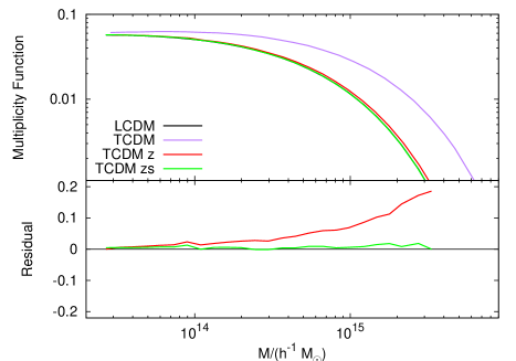
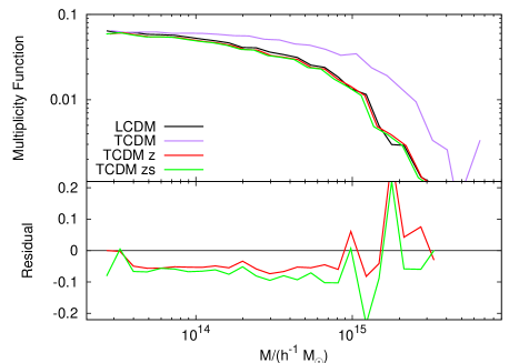
Figure 1: Halo mass functions before and after the scaling procedure. The top panel shows the theoretical mass function of Sheth & Tormen (1999), whereas the bottom panel shows measurements from our simulations (discussed in Section 4). In each panel the mass functions are shown for the target $\Lambda$CDM cosmology (black); the original $\tau$CDM cosmology (purple); the effect of relabelling the redshift of $\tau$CDM (red); and the effect of then also scaling the simulation box size (green), which simultaneously changes individual halo masses. The values of the scaling parameters $z$ and $s$ used to achieve this are given in Table 2 and the details of the simulations are discussed in section 4. We also show the fractional residual between the mass function in the scaled simulations and in the target cosmology; this does not vanish perfectly for the simulation data, indicating that the mass function is not perfectly universal at the few per cent level.

2.1 Matching the mass function

Throughout this paper quantities in the target cosmology are denoted with primes and quantities in the original simulation are unprimed.

The AW10 algorithm first chooses a rescaling in length units of the simulation such that

$$L^{\prime}=sL$$ (1)

and a rescaling in redshift so that outputs in the original simulation at redshift $z$ are matched to a different redshift in the target simulation $z^{\prime}$. Note that we will assume that the box side, $L$, is measured in comoving units, so that $s$ rescales all comoving lengths. We also choose units of $\,h^{-1}\,\mathrm{Mpc}$ for $L$; this is not mandatory, but it simplifies some related scalings, such as that of mass (equation 4). The appropriate powers of $h$ must then be carried in the units of all quantities, such as $\,h^{-1}\,\mathrm{M_{\odot}}$.

For a given $z^{\prime}$, $s$ and $z$ are chosen so as to minimize the difference in the halo mass function between the two cosmologies. To achieve this the RMS difference in the linear variance in density between the two cosmologies is minimized over both $s$ and $z$:

$$\delta_{\mathrm{rms}}^{2}(s,z\mid z^{\prime})=\frac{1}{\ln(R^{\prime}_{2}/R^{\prime}_{1})}\int_{R^{\prime}_{1}}^{R^{\prime}_{2}}\frac{\mathrm{d}R}{R}\left[1-\frac{\sigma(R/s,z)}{\sigma^{\prime}(R,z^{\prime})}\right]^{2}\ ,$$ (2)

where $R^{\prime}_{1}$ and $R^{\prime}_{2}$ are the radial scales, measured in the target cosmology, corresponding to the least massive and most massive haloes in the original catalogue. The radial scale $R$ is given by the radius that would enclose a mass $M$ in a homogeneous Universe,

$$M=\frac{4}{3}\pi R^{3}\bar{\rho}\ ,$$ (3)

where $\bar{\rho}$ is the mean cosmological matter density. Scales in the two simulations are related by $R^{\prime}=sR$; this size rescaling here thus implies a rescaling of the mass via

$$M^{\prime}=s_{\mathrm{m}}M;\quad s_{\mathrm{m}}\equiv s^{3}\frac{\Omega^{\prime}_{\mathrm{m}}}{\Omega_{\mathrm{m}}}\ ,$$ (4)

such that the total mass enclosed in the simulation volume matches the cosmological mass after the rescaling has been applied. Again note that our definition of $M$ includes the units $\,h^{-1}\,\mathrm{M_{\odot}}$.

The linear variance in over-density can be expressed in Fourier space as

$$\sigma^{2}(R,z)=\int_{0}^{\infty}\Delta_{\rm{lin}}^{2}(k,z)T^{2}(kR)\;\mathrm{d}\ln{k}\ ,$$ (5)

where $T(kR)$ is the Fourier transform of a top-hat of radius $R$ which contains a mass $M$ in a homogeneous universe:

$$T(kR)=\frac{3}{(kR)^{3}}(\sin kR-kR\cos kR)\ .$$ (6)

$\Delta_{\rm{lin}}^{2}(k,z)$ is the dimensionless, linear matter power spectrum

$$\Delta_{\rm{lin}}^{2}(k,z)=4\pi V\left(\frac{k}{2\pi}\right)^{3}P(k,z)\ ,$$ (7)

giving the variance per unit $\Delta\ln k$, and where $P(k)$ is the linear power spectrum defined as

$$P(k)=\langle{|\delta_{\mathbf{k}}|^{2}}\rangle\ ,$$ (8)

and $\delta_{\mathbf{k}}$ are the Fourier coefficients of the matter over-density field.

By numerically minimizing equation (2) over $z$ and $s$ one finds a rescaling such that the linear variance of the simulations are as similar as possible to each other across the range of scales that correspond to the mass range of the haloes in the original simulation. This is equivalent to minimizing the difference in halo mass function because, in the simplest models, the mass function depends only on $\sigma$ (Press & Schechter 1974; Sheth & Tormen 1999) as shown in the mass function in equation (15). However, in more complicated models, such as those with collapse thresholds that depend on environment (e.g. Mo & White 1996), this is no longer the case – note also that strong environmentally dependent mass functions are the case for most modified gravity theories (e.g. Lombriser et al. 2013).

The result of this exercise has the issue that the desired value of $z$ will almost certainly not be one of the values stored as a simulation output; alternatively, each stored value of $z$ can be assigned a corresponding $z^{\prime}$, none of which will be exactly the desired target value. In practice, this is not too important: simulation outputs are used to build mock data on a light cone, which always involves some degree of interpolation between outputs. The main thing is that the grid of effective $z^{\prime}$ values is known. The problem can be eased if the outputs from the original simulation are finely spaced in redshift. It can also be an advantage to run this simulation with a high value of $\sigma_{8}$ or alternatively into the future (negative redshifts) in order to produce a large range in fluctuation amplitudes, as this allows the algorithm to find scalings between different cosmological parameters more easily (e.g. Harker et al. 2007, AW10, Ruiz et al. 2011).

It may also be the case that, after remapping, the lowest mass halo in the simulation is too massive to allow generation of a realistic galaxy population. This is a problem with most simulations, where the parent haloes of dwarf galaxies lie below the resolution limit. In all cases, a reconstruction algorithm is thus required, in which the distribution of missing low-mass haloes is inferred from the distribution of the known haloes (e.g. de la Torre & Peacock 2012).

In Fig. 1 we illustrate both the theoretical and measured mass functions at various stages of the scaling process for two rather different example cosmologies. This plot makes use of simulations that are discussed in Section 4 and summarised in Table 1; briefly the two cosmologies are a vanilla $\Lambda$CDM model and $\tau$CDM , a matter only model. Theoretical agreement can be achieved almost perfectly (within 1%) by rescaling, but in the measured mass function there remains some disagreement at around the 5% level. A similar level of disagreement in the measured mass function was found by AW10 (their Fig. 7); this plausibly reflects the fact that the mass function is not perfectly universal (Tinker et al. 2008; Lukić et al. 2007; Manera et al. 2010). We do not use the mass functions of Tinker et al. (2008) because they were calibrated on haloes found with a spherical over-density algorithm (for examples see Knebe et al. 2011) and on a small range of $\Lambda$CDM parameter space. They also have explicit redshift dependence which violates universality, rather than depending only implicitly on redshift via $\sigma$ (equation 5). In principle one could choose $s$ and $z$ to minimise the difference in mass function directly between two different cosmologies and use a more complex $z$-dependent prescription for the mass function, but we have taken the simpler approach for the present paper.

2.2 Matching the displacement field

The second part of the AW10 algorithm involves a shift in the individual particle positions in the rescaled simulation so as to reproduce the large-scale clustering of the target cosmology. This is achieved by taking the linear displacement field in the scaled original cosmology and then using the Zel’dovich Approximation (Zel’dovich 1970; hereafter ZA) to perturb the particle or halo positions: the phase of each mode is preserved, but the amplitude is altered to match the target power spectrum.

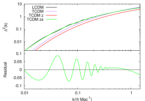
Figure 2: The linear power spectrum of the original and target cosmologies described in Section 4 at each stage of the rescaling process. The black curve shows the target $\Lambda$CDM simulation whereas the other lines show the various stages of the rescaling method: original $\tau$CDM simulation (purple); scaling in redshift (red); and scaling in redshift and size (green). The residual difference in linear power after redshift and size scaling has taken place is shown in the lower panel, this is mainly obvious as the residual wiggle which arises because there is no BAO in the $\tau$CDM model. This difference in linear power is corrected for by modifying particle positions, described in Section 2.2.

Rescaling to match the halo mass function in effect forces the initial simulation to take up the desired linear power spectrum in the region with $\Delta_{\rm{lin}}^{2}\simeq 1$. But in general the target spectrum will not be matched on very different scales. This problem is illustrated clearly in Fig. 2, where the target cosmology has BAO features, whereas the original simulation adopted a zero-baryon transfer function. It is precisely these residual differences in linear power that the next part of the algorithm aims to correct by displacing particles using the ZA.

At each redshift in the target cosmology we define a nonlinear scale $R^{\prime}_{\mathrm{nl}}$ such that

$$\sigma^{\prime}(R^{\prime}_{\mathrm{nl}},z^{\prime})=1\ ;$$ (9)

all fluctuations on scales larger than this are considered to be in the linear regime. AW10 then use this to define a nonlinear wavenumber $k^{\prime}_{\mathrm{nl}}=R_{\mathrm{nl}}^{{}^{\prime}-1}$ that determines which Fourier components of the density field and displacement field are taken to be in the linear regime.

The displacement field $\mathbf{f}$ is defined so as to move particles from their initial Lagrangian positions $\mathbf{q}$ to their Eulerian positions $\mathbf{x}$:

$$\mathbf{x}=\mathbf{q}+\mathbf{f}\ .$$ (10)

At linear order the displacement field is related to the matter over-density $\delta$ via

$$\delta=-\nabla\cdot\mathbf{f}\ ,$$ (11)

which in Fourier space is

$$\mathbf{f}_{\mathbf{k}}=-i\frac{\delta_{\mathbf{k}}}{k^{2}}\mathbf{k}\ .$$ (12)

If the displacement field in the original simulation is known, then an additional displacement can be specified in Fourier space to reflect the differences in the linear matter power spectra between the two cosmologies:

$$\delta\mathbf{f}_{\mathbf{k^{\prime}}}=\left[\sqrt{\frac{\Delta_{\rm{lin}}^{{}^{\prime}2}(k^{\prime},z^{\prime})}{\Delta_{\rm{lin}}^{2}(sk^{\prime},z)}}-1\right]\mathbf{f}_{\mathbf{k^{\prime}}}\ ,$$ (13)

where $\mathbf{f}$ is measured in the original simulation after it has been scaled. Equation (12) is only valid for the linear components of both fields, so in practice the displacement field must be smoothed with a window of width the nonlinear scale $R_{\mathrm{n}l}$.

In AW10 the authors saved the initial displacement field of the simulation and so equation (13) could be used directly to make the required modification of the particle positions. But in the next Section we show how the displacement field can be reconstructed directly from the distribution of haloes in the original simulation.

3 Recasting haloes

The AW10 algorithm produces a new particle distribution, but many practical applications would need to seed this density field with galaxies, for which the first step is locating the dark matter haloes. This takes time, and will also yield incorrect results since the density field is not correct on the smallest scales (i.e. the internal halo properties should change as a result of the altered cosmology). For both these reasons it makes sense to work directly with the halo catalogue. In this section, we therefore show both how the halo catalogue itself can be used to recover the large-scale displacement field (if it is not provided), and we review the changes to the internal halo properties that should be applied after the simulation has been remapped.

(a)

(b)

(c)

(d)

Figure 3: A comparison of the values of the linear displacement fields reconstructed from our scaled (in $s$ and $z^{\prime}$ by the first part of the method) $\tau$CDM simulation (see Section 4). The displacement field is calculated from the density field using equation (12) and debiased in the case of haloes using equation (14). The points show values of the fields in cells for a randomly selected subset (1%) of cells measured on a $75^{3}$ mesh and convolved with a Gaussian to filter out the nonlinear components. The top left panel shows the displacement reconstructed from the particles compared to the original displacement field used to run the simulation. The top right panel shows the same thing but for the displacement field recovered from the debiased halo field. The lower left panel shows the halo displacement field corrected according to equation (20) so as to have the correct theoretical variance. The bottom right panel shows a comparison between this corrected displacement field from haloes and the field from the particles.

3.1 Reconstruction of displacement fields

Following Eisenstein et al. (2007), the displacement field can be obtained from the over-density field using equation (12). This result can be used if we construct the matter over-density field from the haloes, which are biased tracers of the mass distribution. The over-density of haloes $\delta_{\mathrm{H}}$ is related to the matter over-density via the bias $b$:

$$\delta_{\mathrm{H}}=b\delta\ ,$$ (14)

where the bias can, in principle, be a function of mass and other halo properties.

Throughout this work we use the mass function of Sheth & Tormen (1999):

$$f(\nu)=A\left[1+\frac{1}{(q\nu^{2})^{p}}\right]e^{-q\nu^{2}/2}\ ,$$ (15)

where $A=0.216$, $q=0.707$ and $p=0.3$. The mass function is expressed in terms of the variable $\nu=\delta_{\mathrm{c}}/\sigma(M)$ where $\delta_{\mathrm{c}}\simeq 1.686$, which derives from spherical collapse models. $f(\nu)$ is defined such that it gives the fraction of the mass in the Universe in haloes in a range $\nu$ to $\nu+d\nu$. Although more up to date mass functions exist in the literature (Warren et al. 2006; Peacock 2007; Tinker et al. 2008) we choose to use that of Sheth & Tormen (1999) because it was calibrated to simulations that cover a greater range of cosmological parameter space than more modern ones.

Given the mass function, an analytic expression for the linear halo bias can be derived via the peak-background split formalism (Sheth & Tormen 1999):

$$b(\nu)=1-\frac{1}{\delta_{\mathrm{c}}}-\frac{\nu}{\delta_{\mathrm{c}}}\left[\frac{d}{d\nu}\ln f(\nu)\right]\ .$$ (16)

In order to calculate the over-density field from our halo catalogue we take a halo-number weighted ‘effective’ bias for the haloes in the catalogue based on the theoretical models given above in equations (15) and (16):

$$b_{\mathrm{eff}}=\frac{\int_{\nu_{\mathrm{min}}}^{\nu_{\mathrm{max}}}\mathrm{d}\nu\,b(\nu)f(\nu)/m}{\int_{\nu_{\mathrm{min}}}^{\nu_{\mathrm{max}}}\mathrm{d}\nu\,f(\nu)/m}\ ,$$ (17)

where $\nu_{\mathrm{min}}$ and $\nu_{\mathrm{max}}$ are the value of $\nu$ for the least massive and most massive halo in the original simulation.

Nonlinearities in the recovered matter over-density field are limited by convolving the field with a Gaussian whose width is set equal to the nonlinear scale $R_{\mathrm{nl}}$, which can then be converted to a displacement field using equation (12). Our method then proceeds exactly as in AW10: haloes in the original simulation are moved from their old positions $\mathbf{x}$ to new positions $\mathbf{x^{\prime}}$ using the small displacements implied by equation (13)

$$\mathbf{x^{\prime}}=\mathbf{x}+\delta\mathbf{f}\ ,$$ (18)

which follows from equation (10) given that initial positions $\mathbf{q}$ are preserved before and after this final stage of the algorithm. In Fig. 3 we show the displacement fields as predicted from the particle data and from halo catalogues in our simulation (see Section 4). The top left panel shows a comparison between the displacement field reconstructed from the particle distribution with that generated for the simulation initial conditions and we can see that the reconstructed field shows no obvious bias compared to the original fields although there is some scatter. The top right panel then shows the displacement field measured from debiasing the halo density field which shows a small residual bias when compared to the original field. This residual effect possibly reflects a failure of the peak-background bias calculation in the quasi-linear regime. In any case, though, the true expected variance in the smoothed displacement can be calculated:

$$\sigma^{2}_{f}(R_{\mathrm{n}l})=\frac{1}{3}\int_{k_{\mathrm{box}}}^{\infty}\frac{e^{-k^{2}R_{\mathrm{n}l}^{2}}\Delta^{2}_{\mathrm{lin}}(k)}{k^{2}}\;\mathrm{d}\ln k\ ,$$ (19)

where $k_{\mathrm{box}}=2\pi/L$ is the fundamental mode of the simulation. We can therefore scale our displacement fields such that they have the desired variance:

$$\mathbf{f}\rightarrow\mathbf{f}\,\frac{\sigma_{f}(R_{\mathrm{nl}})}{\sqrt{\mathrm{Var}(|\mathbf{f}|)}}\ ,$$ (20)

where $\mathrm{Var}(|\mathbf{f}|)$ is the measured variance in $|\mathbf{f}|$. The result of this scaling can be seen in the bottom left panel of Fig. 3 where there is now better agreement with the original displacement field. The bottom right panel shows a comparison between the reconstructed displacement field from particles and from haloes where there is no obvious disagreement. This shows that our method is able to make a reasonable reconstruction of the full simulation displacement field using only the halo catalogue.

One should note that for a population of lower mass haloes the value of $b_{\mathrm{eff}}$ could be less than 1 and an implementation of equation (14) could then result in cells with negative densities ($\delta<-1$). However, we have checked our reconstruction method for a small volume simulation with a population of low mass haloes with $b_{\mathrm{eff}}\approx 0.83$ and found that it still works as well in reconstructing the displacement field, even though it goes through the unphysical negative density step.

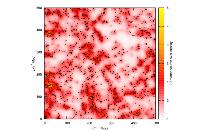
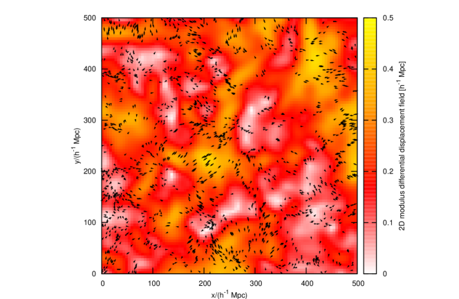
Figure 4: A visual summary of our method. The top panel shows the projected linearized over-density field in a slice of thickness $50\,h^{-1}\,\mathrm{Mpc}$ inferred from the distribution of haloes in our size and redshift scaled $\tau$CDM simulation (described in Section 4) and the bottom panel shows the magnitude of the linearized differential displacement field inferred from the over-density. In each plot the arrows then show the flow of haloes due to the differential displacement field in order to match the clustering in the target $\Lambda$CDM cosmology. The displacements are typically small in the method and the arrows in these plots have been enlarged by a factor of 10 to illustrate the halo flow more clearly.

3.2 Mass-dependent halo displacements

When dealing with the displacement field of haloes, some care is needed in ensuring that these objects display the correct degree of bias as a function of mass. Writing the matter density fluctuation in terms of the displacement field, the linear halo bias relation is

$$\delta_{\mathrm{H}}=-b(M)\nabla\cdot\mathbf{f}\ ,$$ (21)

which says that in effect haloes of different masses are displaced by different amounts. This seems to violate the equivalence principle, and of course all particles in a simulation should share the same displacement field. But this displacement field then affects halo formation in a nonlinear way, which is not allowed for if we subsequently change the displacement field ‘by hand’. In order to obtain the correct statistics of large-scale clustering, the above mass dependence of the effective additional displacement must therefore be respected. To see how the argument works in an extreme case, imagine applying the AW10 method to a simulation with zero-large-scale power. Adding in the large-scale displacement field will then by construction yield a set of haloes that have $b=1$, independent of mass. In order to avoid this unrealistic situation, we have to apply a mass-dependent displacement, as in equation (21).

This argument reveals a subtle limitation of the original AW10 prescription. We can assume that applying a halo finder to a particle distribution that has been subject to the AW10 method will find very much the same haloes as if these were identified prior to the additional displacement, because these displacements are coherent over large scales. These haloes will thus fail to have the correct dependence of clustering on mass. In this respect, our approach is not simply faster than AW10, but working directly with haloes allows a treatment of mass-dependent biasing that is more consistent than can be achieved by scaling the particle distribution alone.

In practice one could bin haloes of differing masses and compute the displacement field for each mass bin individually, thus avoiding the issue of debiasing the over-density and then rebiasing the displacement field. However we choose to use the full halo catalogue to produce the least noisy displacement field possible and then to move haloes of different masses by different amounts according to equation (21).

A visual summary of our method as applied to halo catalogues is given in Fig. 4, in which we show the density and displacement fields as calculated from the halo distribution together with the flow of haloes that these fields imply for our different cosmologies.

3.3 Reconstitution of haloes

The AW10 method reproduces the mass function and linear clustering of the target cosmology, albeit with the small error in mass-dependent halo biasing described above. But in addition, the AW10 approach does not address the deeply nonlinear clustering that arises due to correlations within individual haloes. In Halo Occupation Distribution (HOD) models, galaxies are taken to be stochastic tracers of the mass field around haloes; in order to use rescaling for generation of mock galaxy catalogues, it is therefore necessary to produce the mass field around haloes in a way that reflects the new cosmology. This is also of interest in its own right for applications such as ray-tracing simulations (e.g. Kiessling et al. 2011) for gravitational lensing.

We address this issue by a method of ‘reconstitution’ where the mass distribution around the final set of haloes is calculated by considering how their internal structure should depend on cosmology. We define haloes as spherical objects that have an average over-density with respect to the matter in the background Universe of $\Delta_{\mathrm{v}}\simeq 200$. The use of a fixed density contrast at virialization is motivated by consistency with halo finding methods such as Friends-of-Friends (FoF). The exact value of $\Delta_{\mathrm{v}}$ (motivated by the spherical collapse model) is not critical. The virial radius $r_{\mathrm{v}}$ for a halo of mass $M$ is then

$$r_{\mathrm{v}}=\left(\frac{3M}{4\pi\Delta_{\mathrm{v}}\bar{\rho}}\right)^{1/3}\ .$$ (22)

Haloes differ between cosmologies in having different density profiles; this can be traced to the haloes having different collapse redshifts, via the differing growth rate of perturbations (Navarro et al. 1997; Bullock et al. 2001; Eke et al. 2001). Although we have defined haloes to have a fixed virial radius for a given mass, the concentration of haloes (ratio of virial radius to internal characteristic radius) does vary as a function of cosmology. The density profiles of haloes have been claimed to be universal (Navarro et al. 1997) with a functional form of

$$\rho(r)=\frac{\rho_{\mathrm{N}}}{(r/r_{\mathrm{s}})(1+r/r_{\mathrm{s}})^{2}}\ ,$$ (23)

where $r$ is the distance from the halo centre, $r_{\mathrm{s}}$ is a scale radius and $\rho_{\mathrm{N}}$ is a normalization to obtain the correct halo mass. Although subsequent work (Merritt et al. 2005; Merritt et al. 2006) showed this form to be imperfect at small $r$, it will suffice for our present purpose: mock galaxies are either central at $r=0$ exactly, or satellites that tend to be found around $r_{\mathrm{s}}$, where the NFW approximation is good. The density profile is truncated at the virial radius $r_{\mathrm{v}}$, which is determined by the halo mass (equation 22); the density profile is therefore fully specified via a value for $r_{\mathrm{s}}$ or alternatively for the halo concentration $c=r_{\mathrm{v}}/r_{\mathrm{s}}$.

We choose to use the cosmology dependent concentration relations of Bullock et al. (2001) for convenience; these are defined as a function of redshift $z$ to be

$$c(z,z_{\mathrm{c}})=4\left(\frac{1+z_{\mathrm{c}}}{1+z}\right)\ ,$$ (24)

where $z_{\mathrm{c}}$ is a collapse redshift which depends on halo mass, calculated via

$$\frac{g(z_{\mathrm{c}})}{g(z)}\,\sigma(0.01M,z)=\delta_{\mathrm{c}}\ ,$$ (25)

where $g(z)$ is the linear growth factor normalized to $1$ at $z=0$. This expression gives the redshift at which the halo has gathered $1\%$ of its current mass. Since both $\sigma$ and $g$ depend on cosmology, the halo concentrations depend on cosmology, with more massive haloes collapsing later and being consequently less concentrated. The concentration relations of Bullock et al. (2001) were calibrated using haloes whose virial radius was defined to vary as a specific function of cosmology according to the spherical model approximation of Bryan & Norman (1998).

$$\Delta_{\mathrm{v}}^{\mathrm{B}}(z)=\frac{178-82[1-\Omega_{\mathrm{m}}(z)]-39[1-\Omega_{\mathrm{m}}(z)]^{2}}{\Omega_{\mathrm{m}}(z)}\ .$$ (26)

As argued above, this may not be the correct choice in detail when using FoF haloes with a cosmology-independent linking length, and the appropriate value is probably best measured empirically in a given simulation (see Section 3.4). In this case one should modify the Bullock et al. (2001) value for the concentration at given mass:

$$\left[\ln(1+c)-\frac{c}{1+c}\right]=\frac{\Delta_{\mathrm{v}}}{\Delta_{\mathrm{v}}^{\mathrm{B}}}\frac{c^{3}}{c_{\mathrm{B}}^{3}}\left[\ln(1+c_{\mathrm{B}})-\frac{c_{\mathrm{B}}}{1+c_{\mathrm{B}}}\right]\ .$$ (27)

Unless otherwise stated, we adopt $\Delta_{\mathrm{v}}=200$ as a default value. This choice is not critical, since we are often interested in differential effects between cosmologies, and the main cosmology dependence of halo properties comes through the influence on the concentration of altered formation redshifts.

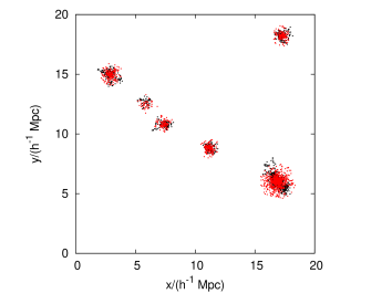
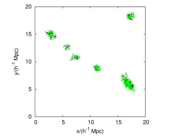
Figure 5: The particles in a small cube of the $\tau$CDM simulation of side length $20\,h^{-1}\,\mathrm{Mpc}$ that were grouped into haloes by our FoF algorithm are shown in black. In the top panel overplotted in red are our reconstituted spherical NFW haloes; in the bottom panel our reconstituted aspherical NFW haloes are shown in green, and these clearly match the haloes in the simulation much better.

One can use the information in this section to reconstitute the particles contained in each halo by calculating the virial radius and concentration parameter for each halo in the catalogue and then filling up the density profile around the halo by a random sampling of tracer particles which correspond to those in the original simulation. A pictorial representation of this is shown in Fig. 5 where haloes measured in a simulation with a FoF algorithm (see Section 4) are shown together with those reconstituted using the halo catalogue generated from this distribution.

The top panel of Fig. 5 shows that ‘real’ haloes are often far from spherical, so it is better to reconstitute them as triaxial objects. This is done using the moment of inertia tensor

$$I_{ij}=\sum_{k=1}^{N}(x_{k,i}-\bar{x}_{i})(x_{k,j}-\bar{x}_{j})\ ,$$ (28)

where $k\in\{1,...,N\}$ and there are $N$ particles in each halo and $i,j\in\{1,2,3\}$ and label coordinates. We work with haloes of 100 particles or more which we consider to be adequate for estimating this tensor. Diagonalizing this tensor provides the axis ratios of the halo (via the eigenvalues) and the orientation of the halo (via the eigenvectors). The eigenvalues and eigenvectors are stored when we generate the halo catalogue from the particle distribution. Asphericity is then restored to the haloes by distorting them once they have been generated by the spherical halo reconstitution process described above. If the square roots of the eigenvalues are $a$, $b$ and $c$ then each coordinate of the reconstituted halo in the centre of mass frame is modified according to

$$x_{i} \rightarrow 3ax_{i}/(a+b+c)\ ,$$

$$y_{i} \rightarrow 3by_{i}/(a+b+c)\ ,$$

$$z_{i} \rightarrow 3cz_{i}/(a+b+c)\ .$$ (29)

We also considered the prescription $x\rightarrow ax/(abc)^{1/3}$ etc. but found this not to work as well in recovering the shapes of aspherical haloes. The CM position vector of each halo particle is then rotated by the inverse matrix of eigenvectors in order to orient the halo correctly.

In the top panel of Fig. 6 we show the power spectrum of the particles in haloes after they have been reconstituted from a halo catalogue, and we compare this to the power spectrum of the particles in haloes in the original simulation that was used to create the catalogue. Clearly the clustering will agree on large scales, but it is satisfying to see that the power spectrum of the particles in haloes can be reproduced by generating our own NFW haloes even out to relatively small scales ($k\simeq 1\,h\,\mathrm{Mpc}^{-1}$). One can see that there is also a significant improvement in the matching in the clustering gained by reconstructing aspherical haloes rather than purely spherical ones.

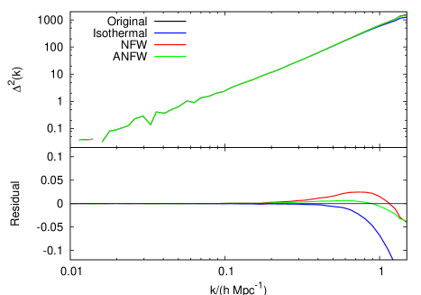
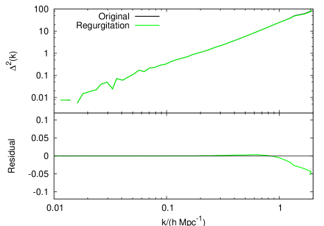
Figure 6: The top panel shows the power spectrum of particles in haloes. We show spectra of the particles in the original haloes in our $\Lambda$CDM simulation (black) together with the power of spherical (red) and aspherical (green) NFW haloes generated from the halo catalogue via the halo reconstitution process described in the text. There is a clear improvement in the match of the power spectra gained from using aspherical rather than spherical haloes. Also shown for comparison is the power spectrum for a more unrealistic halo: the singular isothermal sphere (blue); this fails to match the target even at fairly large scales. In the lower panel we show the full matter power spectrum after we have regurgitated our reconstituted haloes back into the parent particle distribution. One can see the match is essentially perfect to around $k=1\,h\,\mathrm{Mpc}^{-1}$. The 5% drop in power at smaller scales in both panels may reflect either imperfect concentration relations or lack of halo substructure in our reconstitution.

The final idea we consider is a method of ‘regurgitation’, in order to recreate the full mass distribution in the best possible way. Once the original AW10 algorithm has been applied to a full particle distribution, haloes are then selected and removed from the particle distribution and then reconstituted in the same way as described above. These reconstituted haloes, with the correct internal structure for the new cosmology, are then reinserted into the rescaled mass distribution in order to produce a corrected full particle distribution for the new cosmology. In doing this we avoid the problem of discontinuities between the reconstituted halo and the surrounding material by using a constant $\Delta_{\mathrm{v}}$ for our haloes so that they have identical virial radii independent of cosmology. One should note that a limitation of this approach is that we move all particles in the simulation according to the same displacement field and so haloes are not subject to the biased displacements discussed in Section 3.2. This is a general limitation of the AW10 method when one deals with the particle distribution rather than the halo distribution.

The lower panel of Fig. 6 shows the full matter power spectrum measured in a perfect test case where no rescaling has taken place. Haloes have been identified with a FoF algorithm and removed from the particle distribution. This halo catalogue is then used to reconstitute haloes and these are then regurgitated back into the surrounding particle distribution of the simulation. The power spectrum is able to be recreated perfectly up to $k=1\,h\,\mathrm{Mpc}^{-1}$ where deviations arise, possibly due to lack of substructure or imperfect concentration relations in the reconstituted haloes. It should be possible to improve this situation by using the exact 3D particle distribution of the haloes, and scaling radii according to the different concentrations in the two cosmologies. We have not pursued this in detail here, since our focus is on seeing how much can be achieved using halo catalogues alone.

3.4 Scaling velocities

All the discussion so far has been in configuration space. But galaxy surveys inhabit redshift space, in which the clustering signature is modified by peculiar velocities. This distortion is well-known to be an invaluable source of additional cosmological information, giving direct access to the growth rate of density perturbations (Kaiser 1987; Reid et al. 2012). We therefore now give a discussion on how to scale particle and halo velocities.

The main element of scaling of velocities in cosmological simulations is explained in Section 15.7 of Peacock (1999). Since a computational volume has no knowledge of the physical size that it is intended to represent, the natural measure of velocity is ${\mathbf{U}}\equiv{\mathbf{v}}/HaL$, i.e. peculiar velocity in units of expansion across the box (whose proper size is $aL$). According to the Zel’dovich approximation, $\mathbf{U}$ is equal to the displacement field in units of the box size, times the logarithmic growth rate $f_{\mathrm{g}}\equiv\mathrm{d}\ln\delta/\mathrm{d}\ln a\simeq\Omega^{0.55}_{\mathrm{m}}(a)$ (where the latter approximation applies for a flat $\Lambda$-dominated model). In other words, for two simulations that have identical fluctuation spectra in box units (which is exactly true by definition in reinterpreting an original simulation output), we would expect the value of $\mathbf{U}$ to be unaffected by a change in cosmology, apart from the alteration in $f_{\mathrm{g}}$. The recipe for rescaling large-scale peculiar velocities is thus

$$\mathbf{v}^{\prime}=s\frac{H^{\prime}f^{\prime}_{\mathrm{g}}a^{\prime}}{Hf_{\mathrm{g}}a}\mathbf{v}\ .$$ (30)

This argument does not apply on small scales, where velocities are due predominantly to bound motions in haloes. But the error is not large: according to the ‘cosmic virial theorem’ of Section 75 of Peebles (1980), the pairwise peculiar velocity dispersion for a given level of mass clustering scales as $\Omega_{\mathrm{m}}^{0.5}$. Therefore, simply rescaling the velocities according to linear theory would give a result in error on small scales by only about 7%, even when rescaling from $\Omega_{\mathrm{m}}=1$ to $\Omega_{\mathrm{m}}=0.25$.

However, the above scaling does not account for the large-scale modifications to displacement fields as discussed in Section 2.2. in the Zel’dovich approximation, peculiar velocities are assigned to particles by

$$\mathbf{v}=aHf_{\mathrm{g}}\mathbf{f}\ ,$$ (31)

we can therefore impose additional differential changes on the peculiar velocities of particles via

$$\delta\mathbf{v}_{\mathbf{k^{\prime}}}=a^{\prime}H^{\prime}f_{\mathrm{g}}^{\prime}\left[\sqrt{\frac{\Delta_{\rm{lin}}^{{}^{\prime}2}(k^{\prime},z^{\prime})}{\Delta_{\rm{lin}}^{2}(sk^{\prime},z)}}-1\right]\mathbf{f}_{\mathbf{k^{\prime}}}\ .$$ (32)

In this and the earlier discussion, it should be kept in mind that the velocities are in proper units, but ${\bf f}$ is a comoving displacement field; this accounts for the extra factor of $a$. Note that this additional velocity is applied independent of halo mass, unlike the mass-dependent displacement discussed earlier. The latter step was needed to preserve the mass-dependent biasing, but velocities of haloes have no such mass dependence. Therefore, in effect, it is necessary to break the Zel’dovich approximation in order to ensure correct large-scale statistics.

In addition, the velocity of particles in haloes will be different in the new cosmology. The circular velocity at a radius $r$ from the centre of a halo of mass $M$ can be calculated for an NFW profile:

$$v_{\mathrm{circ}}^{2}(r)=\frac{GM}{r}\left[\frac{\ln(1+r/r_{\mathrm{s}})-\frac{r/r_{\mathrm{s}}}{1+r/r_{\mathrm{s}}}}{\ln(1+c)-\frac{c}{1+c}}\right]\ ,$$ (33)

where $G$ is the gravitational constant. If the halo particles themselves are restructured, then velocities can be assigned to particles in haloes in a differential way:

$$\mathbf{v^{\prime}}=\mathbf{v}\frac{v^{\prime}_{\mathrm{circ}}(r^{\prime})}{v_{\mathrm{circ}}(r)}\ .$$ (34)

More normally, we might lack any internal halo velocity data, in which case the velocities would need to be generated by hand. The simplest approximation would be to assume isothermal and isotropic orbits; this is not consistent, and more detailed modelling could be carried out based on the Jeans Equation, together with assumptions about orbital anisotropy. But for the present, we shall go no further than noting that virial equilibrium and isotropy yields an rms line-of-sight velocity dispersion for an NFW halo of

 

$${\sigma_{v}^{2}}$$

  (35)

This can be compared with $\sigma_{v}^{2}=GM/3r_{\mathrm{v}}$ for the truncated singular isothermal sphere. We found that equation (35) with $\Delta_{\mathrm{v}}=200$ under-predicts halo velocity dispersions in $\Lambda$CDM simulations by a factor of around 1.07, implying that $\Delta_{\mathrm{v}}\simeq 300$ would be a better practical choice for this application. Better still, if a halo velocity dispersion is included in a catalogue, then a scaled version of this value can be used directly to reconstitute halo particles with the correct dispersion.

3.5 Method summary

Here we provide a brief summary of a practical implementation of our method for use on a halo catalogue:

1. Calculate $z$ and $s$ by minimizing equation (2) over the mass range of haloes in the original halo catalogue.

2. Calculate the effective bias for the haloes using equation (17).

3. Calculate the matter over-density field implied by the halo catalogue, taking care to debias the halo field appropriately.

4. Linearize the matter over-density field using a Gaussian with width of the nonlinear scale, defined in equation (9).

5. Compute the displacement field from the over-density field using equation (12) and then correct this so that it has the correct theoretical variance using equation (20).

6. Taking the original catalogue at redshift $z$, relabel positions of haloes according to equation (13). This new catalogue can then be interpreted as a catalogue of haloes in the target cosmology at redshift $z^{\prime}$, complete with new halo properties.

7. If desired, reconstitute the particles in haloes using the method detailed in Section 3.3.

4 Simulations

We illustrate our method using a matched set of simulations and the halo catalogues generated from them. The simulation parameters are given in Table 1. The ‘target’ simulation $\Lambda$CDM is a WMAP1 style cosmology (Spergel et al. 2003) run with the same transfer function as that of the Millennium Simulation (Springel et al. 2005) which was generated using CMBFAST (Seljak & Zaldarriaga 1996). The ‘original’ simulation $\tau$CDM is a flat matter-only simulation run with a defw transfer function (Davis et al. 1985) tuned to have a similar spectral shape to that of the Millennium Simulation. $\tau$CDM models were popular in the past as a way of enabling flat matter only models to fit clustering data from contemporary galaxy surveys (e.g. the APM survey: Maddox et al. 1990) whose spectral shape appeared to require a sub-critical mass density. The $\tau$CDM model of White et al. (1995) dealt with this by introducing extra relativistic species, thus changing the epoch of matter radiation equality without lowering the mass density.

Initial conditions were generated for each simulation by perturbing particle positions from an initial glass configuration of $512^{3}$ particles using the N-GenIC code at an initial redshift of $z_{\mathrm{i}}=199$. The simulations themselves were run using the cosmological $N$-body code Gadget-2 of Springel (2005). Performing direct test simulations allows us to use the same phases for the Fourier modes in the target and original simulations, so that the approximate and exact target halo fields can be compared visually, and not just at the level of power spectra. This also allows us to analyse the results of the rescaling without the added complication of cosmic variance.

Table 1: Cosmological parameters for our simulations. As a ‘target’ we use a $\Lambda$CDM model with a WMAP1 type cosmology and as an ‘original’ model we simulate a matter only model with a defw (Davis et al. 1985) spectrum with a similar spectral shape ($\Gamma=0.21$) to that of the $\Lambda$CDM model but that lacks a BAO feature. Each simulation ran with $512^{3}$ particles, gravitational forces were softened at $20\,h^{-1}\,\mathrm{kpc}$ and initial conditions generated using N-GenIC on an initial glass load at a starting redshift $z_{\mathrm{i}}=199$.

Simulation	$L$	$\Omega_{\mathrm{m}}$	$\Omega_{\Lambda}$	$\Omega_{\mathrm{b}}$	$h$	$\sigma_{8}$	$n_{\mathrm{s}}$	$\Gamma$
$\Lambda$CDM	$780\,h^{-1}\,\mathrm{Mpc}$	0.25	0.75	0.045	0.73	0.9	1	-
$\tau$CDM	$500\,h^{-1}\,\mathrm{Mpc}$	1	0	-	0.5	0.8	1	0.21

Table 2: Best fit scaling parameters for scaling between our original $\tau$CDM model and our target $\Lambda$CDM model.

Original	Target	$z$	$z^{\prime}$	$s$	$M_{1}$	$M_{2}$	$s_{\mathrm{m}}$	$k_{\mathrm{nl}}$	$b_{\mathrm{eff}}$
$\tau$CDM	$\Lambda$CDM	0.22	0	1.56	${2.58}\times 10^{13}\,h^{-1}\,\mathrm{M_{\odot}}$	${3.41}\times 10^{15}\,h^{-1}\,\mathrm{M_{\odot}}$	0.95	$0.15\,h\,\mathrm{Mpc}^{-1}$	1.59

Our procedure for generating the simulations was as follows: run the original simulation to $z=0$ in a box of size $L$, compile a halo catalogue and then use the mass range in this halo catalogue to compute the best scaling parameters ($s$, $z$) by minimising equation (2). We then re-ran the original simulation to redshift $z$ because this used comparatively little computational resources. However, in practice one would interpolate particle positions between simulation outputs around redshift $z$ if one was interested in particles, or constrain the scaling redshift to be one of a set of $z$ (close to the best fit) for which one already had an output. This would be necessary in the case of halo catalogues because it is not obvious how to interpolate haloes between catalogues due to mergers. For the purpose of comparisons we also ran a simulation of the target cosmology to $z^{\prime}=0$ in a box of size $L^{\prime}=sL$ and compiled a halo catalogue. In doing this step we chose the same random numbers for the mode phases and amplitudes for the realization of the displacement fields to ensure that structures appear in the same point in both simulations, despite the different box sizes. This allowed for direct comparisons between the simulation particle distributions and halo catalogues that are affected only by the different background cosmologies rather than by cosmic variance.

We compile halo catalogues using the public FoF code www-hpcc.astro.washington.edu/tools/fof.html with a linking length of $0.2$ times the mean inter-particle separation in the simulation. We catalogue only haloes that contain $\geq 100$ particles and we define halo centres to be the centre of mass of all contributing halo particles.

For our simulations the best-fit scaling parameters are given in Table 2. Fig. 1 shows the effect of each stage of the scaling on the halo mass functions; the theory of Sheth & Tormen (1999) is shown in the top panel, whereas the effect on the measured mass functions is shown in the bottom panel. The scaling makes the theoretical predictions for the mass functions agree to within 1%, but this agreement is less perfect for the measured mass functions, which display discrepancies of up to 10%. This discrepancy can be traced back to the fact that the fitting formula for the mass functions of Sheth & Tormen (1999) are only accurate to 20% and that the mass function is only ‘nearly’ universal (Tinker et al. 2008; Lukić et al. 2007). A similar level of disagreement in the measured mass function was found in AW10 (their Fig. 7) in converting between WMAP1 and WMAP3 cosmologies.

Throughout this work we measure power spectra by creating the density field on a mesh by assigning particles to mesh cells with a nearest grid point mass assignment scheme and then taking the Fourier transform of this density field. The effect of our binning in cubic cells is corrected for by deconvolving the final Fourier transform with the normalized transform of a cubic cell,

$$J(k)=\mathrm{sinc}\,{(\theta_{x})}\,\mathrm{sinc}\,{(\theta_{y})}\,\mathrm{sinc}\,{(\theta_{z})}\ ,$$ (36)

where $\theta_{i}=k_{i}L/2m$ and $m$ is the number of mesh cells used for the density field. The power is thus adjusted according to

$$\Delta^{2}(k)\rightarrow\frac{\Delta^{2}(k)}{J^{2}(k)}\ .$$ (37)

We compute power spectra of both haloes and particles. In each case we assume that these discrete objects randomly sample the (biased in the case of haloes) mass field so we subtract shot noise from the power in each case. This implies

$$\Delta^{2}(k)\rightarrow\Delta^{2}(k)-4\pi\left(\frac{k}{2\pi}\right)^{3}\frac{L^{3}}{N}\ ,$$ (38)

where $N$ is the total number of particles in the simulation. This correction is only important at small scales, where the shot noise correction has been shown to be valid even for glass initial conditions (Smith et al. 2003).

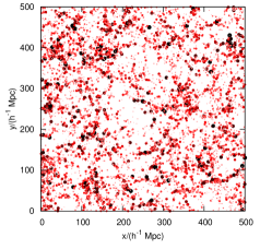
(a)

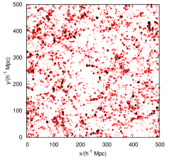
(b)

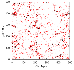
(c)

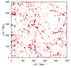
(d)

Figure 7: A pictorial summary of our results for the rescaling of a halo catalogue. The figures all show the halo distribution in $500\times 500\,(\,h^{-1}\,\mathrm{Mpc})^{2}$ slices of thickness one tenth of the box size ($50\,h^{-1}\,\mathrm{Mpc}$ for the upper two panels and $78\,h^{-1}\,\mathrm{Mpc}$ for the lower two) through different sections of our simulations. All panels show the haloes above ${2.6}\times 10^{13}\,h^{-1}\,\mathrm{M_{\odot}}$ with a point size and colour that depends on halo mass. The top left panel shows the halo distribution at redshift 0 in the $\tau$CDM simulation. The top right panel shows the distribution at redshift $z=0.22$ which is visibly less evolved. The bottom left panel shows the result of the full scaling algorithm; this mainly has the effect of a zoom owing to the scaling of box size and halo mass ($L\rightarrow 1.56L$ and $M\rightarrow 0.95M$), plus a shifting of haloes to reproduce the correct clustering according to the ZA. In fact, the ZA displacement is hard to detect by eye, but Fig. 9 shows that it has a major impact on the halo power spectrum. The bottom right panel shows the excellent agreement with the final halo distribution at redshift 0 in a directly constructed target $\Lambda$CDM simulation, using the same phases as the rescaled $\tau$CDM box.

5 Results from simulations

A visual summary of our rescaling method is given in Fig. 7, where the distribution of haloes is shown at each stage of the rescaling method. This illustrates the good agreement between the distribution of haloes in the fully scaled original halo catalogue and those in the target catalogue. This comparison is facilitated by the fact that we are able to use the same phases in the initial conditions for the two simulations, so that any differences in appearance should reflect only the treatment of nonlinear structure formation.

As a first test of our method we aim to reproduce the AW10 results for the power spectrum of the matter over-density field and these are shown in Fig. 8. This is exactly the AW10 algorithm except that we have regenerated the displacement fields from the particle distribution directly. In these plots the full algorithm has been applied to the particle distribution. The top panel shows the measured power spectra at each stage of the scaling: One can see that the BAO signal in the residual is completely removed by modifying the particle positions and that the measured power spectra agree at the 1% level out to $k=0.15\,h\,\mathrm{Mpc}^{-1}$. Beyond this the power spectra disagree at around the 20% level, reflecting the fact that the interior structure of the haloes has not been altered to account for the change in background cosmology. We correct for this using our reconstitution technique below. With this exception, it is impressive that quite a broad shift in cosmological parameters (see Table 1) can be dealt with by the AW10 algorithm. This includes the generation of a BAO feature in the particle distribution as well as the inclusion of vacuum energy – even though the results are based on the matter-only $\tau$CDM simulation. This test is in very good agreement with AW10 and provides a useful independent confirmation of the accuracy of their algorithm. We have also compared the power spectrum obtained when using the original displacement field from the simulation (i.e. the original AW10 method), rather than reconstructed one, and we found negligible difference. This is good given the scatter in the comparison of the displacement field see in Fig. 3. The bottom panel in Fig. 8 shows an analytical halo model prediction for the full matter power spectrum, where we can see that the form of the rescaled residual is very similar to that in the top panel. This motivates our assertion that the remaining small-scale differences are due to the treatment of halo internal structure.

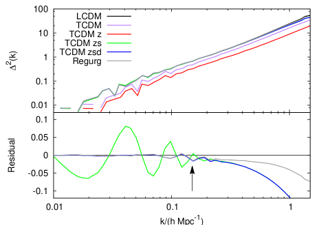
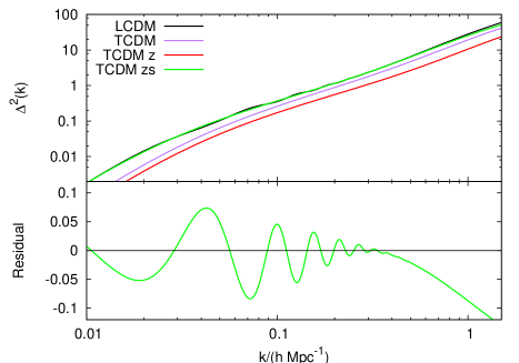
Figure 8: The top panel shows the matter power spectra measured in the simulations at various stages of the method scaling between the $\tau$CDM and $\Lambda$CDM simulations. The black line is the target $\Lambda$CDM power spectrum whereas the other lines show the various stages of the method, original $\tau$CDM simulation (purple), scaling in redshift (red), scaling in redshift and size (green), full AW10 scaling including position modifications using the displacement fields (blue) and finally a power spectrum in which haloes have been removed from the scaled simulation and replaced with aspherical haloes of the correct concentrations for this cosmology (regurgitation, gray). One can see that adjusting particle positions using the ZA almost completely removes the residual BAO feature in the power spectrum, leaving the agreement between simulations at the level of $1\%$ up to the nonlinear scale (black arrow, equation 9). Replacing haloes with those of the correct concentrations improves the match to the target simulation at small scales leaving the agreement at the level of $10\%$ up to $k=2\,h\,\mathrm{Mpc}^{-1}$. The lower panel shows the predicted differences for the full matter power spectrum given by a halo model calculation. The discrepancy seen at small scales in the halo model implies that this is due to halo internal structure and thus provides justification for modifying the halo internal properties.

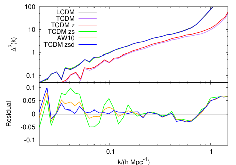
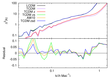
Figure 9: The power spectrum of haloes at each stage of the rescaling procedure. We shows the target $\Lambda$CDM spectrum of haloes (black) and the original halo catalogue at each stage of the scaling process, the original catalogue at $z=0$ (purple), the redshift scaled $\tau$CDM (red), $\tau$CDM with both box size relabelled and redshift changed (green) and finally the result of also then modifying the halo positions according to the ZA. We do this in two distinct ways: applying the same differential displacement field to all haloes (AW10; orange), and giving different haloes a biased version of this displacement according to mass (blue) The upper panel shows the number weighted spectrum of haloes above ${2.6}\times 10^{13}\,h^{-1}\,\mathrm{M_{\odot}}$ while the lower panel shows that of haloes above ${5}\times 10^{13}\,h^{-1}\,\mathrm{M_{\odot}}$. In both cases, we can see that the universal displacement leaves a residual that reflects the BAO signal, whereas the mass-dependent displacement removes this problem entirely, leaving agreement in both spectra at the level of $5\%$ or better except at the largest scales shown where the match is degraded slightly.

A more demanding test of rescaling is to ask if the method can reproduce the desired clustering of haloes. The results of our method of directly scaling a halo catalogue are shown in Fig. 9 as the number weighted power spectra of haloes above ${2.6}\times 10^{13}\,h^{-1}\,\mathrm{M_{\odot}}$ in the upper panel and the number weighted spectra of those above ${5}\times 10^{13}\,h^{-1}\,\mathrm{M_{\odot}}$ in the lower panel at each stage of the scaling process. The displacement field required to move haloes around according to the ZA has been generated entirely from the halo distribution using the method described in the text. Without this displacement, the power spectra are clearly in error, with a residual that reflects the BAO signal. This error is reduced when we apply the differential displacement field to the haloes, but it is not eliminated. However, if the displacement applied to each halo is scaled according to the mass-dependent bias, $b(M)$, this problem is cured. This confirms the need to apply a mass-dependent differential displacement to haloes, an aspect which is absent in the original AW10 algorithm. As a further test of this point, we explicitly calculated the mass-dependent bias to see if this was better recovered with our method. But in practice the results were noisy (few haloes) and we are looking for small shifts in a bias that is already well matched, however, we believe the improved match in Fig. 9 is difficult to attribute to anything other than an improved match in bias. At the largest scales shown the rescaling method seems to degrade the match slightly and we are unsure why this is. However, we see the same effect when we tested the method on smaller volume simulations at the largest scales probed by those simulations, scales that the method shown in Fig. 9 corrects well, so this is plausibly to do with resolution on scales of order the box size.

Figure 10: The power spectra of only particles residing in haloes. We show spectra of the particles in the original haloes in the target simulation (black) together with particles in haloes reconstituted from the original catalogue that are spherical (red), aspherical (green). The orange curve shows the result of using the original AW10 method and aspherical haloes. Haloes are dressed with NFW profiles with concentration relations described in the text. There is a clear improvement gained by using a bias dependent displacement field and by using aspherical haloes over spherical haloes. The maximum error here does not exceed $6\%$.

The final part of our investigations involves reconstituting the particles in haloes using only the halo catalogues. In order to do this we compare the power spectrum of only the particles in haloes reconstituted from the scaled $\tau$CDM halo catalogue to the power spectrum of particles in the haloes in the $\Lambda$CDM simulation. This is shown in Fig. 10, which again displays good agreement (the spectra agree to 5% across the range of scales shown) by using the full scaling algorithm. Clearly there is an improvement on small scales gained by using aspherical haloes over spherical ones.

Finally we look at our regurgitation method in which, after the original AW10 scaling method has been applied to particle data, the haloes are located with FoF, removed and then replaced by reconstituted haloes with corrected mass-concentration relations. The results of this were shown above in the form of the power spectrum in Fig. 8, where we see that the agreement between the original and target cosmologies is much improved by this method at scales above $k=0.1\,h\,\mathrm{Mpc}^{-1}$ due to our modifications of the haloes’ internal structure. Thus the final fully rescaled power spectra agrees at a sub percent level to $k=0.1\,h\,\mathrm{Mpc}^{-1}$ and to a 5% level out to $k=1\,h\,\mathrm{Mpc}^{-1}$. Here there is a clear improvement over the original AW10 algorithm, gained by manipulating the properties of individual haloes.

6 Conclusions

In this paper we have demonstrated that the rescaling method of Angulo & White (2010) may be modified so as to apply directly to halo catalogues. We made an AW10 rescaling of length, mass, and redshift as well as using the halo positions themselves to compute the displacement fields (by debiasing the halo over-density fields), in order to correct the linear clustering in the simulation using the Zel’dovich approximation. This method enables rapid scaling of a halo catalogue to a different cosmology, and is entirely self-contained, being based only on the halo catalogue. We note that this provides a dramatic increase in speed when using the halo catalogue alone. Computational effort is only really used when reading the catalogue into memory and when computing the Fourier Transforms for the displacement field correction. In our case the halo catalogue was small, containing only $\sim 70,000$ haloes, and a Fourier mesh of only $75^{3}$ was all that was required to resolve the linear components of the displacement field. This resulted in a total run time for the rescaling of only a few seconds on a standard desktop computer. This would increase for larger volume halo catalogues because more mesh cells would be required to resolve the linear fields, and for larger halo catalogues, but it is obviously many orders of magnitude faster than running a new simulation.

Working with haloes has the advantage of speed, but also allows two improvements on the original AW10 method. The first of these concerns the internal structure of haloes, which depends on cosmology. This can be allowed for by ‘reconstituting’ the halo internal density distribution using analytical profiles and scaling relations appropriate for the target cosmology. If the catalogue of halo particles is available, it is also possible to ‘regurgitate’, in which haloes are replaced with those with the correct internal structure for the new cosmology.

The other issue applies on large scales. The AW10 method applies an additional displacement in order to ensure that the large-scale linear clustering is as desired in the target cosmology. But applying this extra displacement to all haloes, independent of their mass, will not yield the correct mass-dependent bias, $b(M)$. We found that better results were obtained at the level of the power spectrum by scaling the extra displacement in a mass-dependent way. Clearly this is a minor issue if the original and target cosmologies are close to each other, but it may be important in spanning a large parameter space.

We have tested our method by rescaling a halo catalogue generated from a matter-only $\tau$CDM simulation into that of a more standard $\Lambda$CDM model. This represents a radical shift in cosmology, especially considering that the initial simulation contains no dark energy. At the level of the particle distribution the matter power spectrum is predicted correctly after the rescaling to the level of 1% to $k=0.2\,h\,\mathrm{Mpc}^{-1}$ and 10% to $k=1\,h\,\mathrm{Mpc}^{-1}$. This is in excellent agreement with the original AW10 results and provides independent confirmation of the accuracy of the scaling algorithm. For the haloes the power spectra are noisier, but are still predicted correctly at the level of 10% up to $k=0.2\,h\,\mathrm{Mpc}^{-1}$ with no obvious biases. We have also tested reconstitution of haloes, showing that this method is able to reproduce the power spectrum of particles in haloes at the level of 2% at $k=1\,h\,\mathrm{Mpc}^{-1}$ in the perfect case (no rescaling, simply comparing reconstituted halo particles to those originally used to compile the catalogues) and 7% in the case of our reconstitution of the rescaled haloes. By replacing haloes in a scaled particle distribution via ‘regurgitation’, a further improvement is gained over the original AW10 algorithm, leaving the agreement in matter power spectra essentially perfect at scales below $k=0.1\,h\,\mathrm{Mpc}^{-1}$ and agreeing to within 5% to $k=1\,h\,\mathrm{Mpc}^{-1}$. More demanding tests of the method are certainly possible; in future work we aim to consider aspects beyond the power spectrum, for example higher-order statistics or details of the differences in position between rescaled and target haloes.

We have also provided a method for rescaling velocities, although a detailed investigation of the operation of this method in redshift space will be given elsewhere. Another interesting line of investigation would be to see if the displacement field can be better reproduced from the halo distribution by looking at different reconstruction techniques. Further work could also examine the effect of different mass-concentration relations for the haloes or different non-universal prescriptions for the mass function. Even so, the current method already seems well suited for the application of rapid generation of mock galaxy catalogues covering a wide range of cosmologies.

References

- Anderson et al. (2013) Anderson L. et al., 2013, ArXiv: 1303.4666
- Angulo & White (2010) Angulo R. E., White S. D. M., 2010, MNRAS, 405, 143
- Baugh (2006) Baugh C. M., 2006, Reports on Progress in Physics, 69, 3101
- Bernardeau et al. (2002) Bernardeau F., Colombi S., Gaztañaga E., Scoccimarro R., 2002, Physics Reports, 367, 1
- Bryan & Norman (1998) Bryan G. L., Norman M. L., 1998, ApJ, 495, 80
- Bullock et al. (2001) Bullock J. S., Kolatt T. S., Sigad Y., Somerville R. S., Kravtsov A. V., Klypin A. A., Primack J. R., Dekel A., 2001, MNRAS, 321, 559
- Davis et al. (1985) Davis M., Efstathiou G., Frenk C. S., White S. D. M., 1985, ApJ, 292, 371
- de la Torre et al. (2013) de la Torre S. et al., 2013, ArXiv: 1303.2622
- de la Torre & Peacock (2012) de la Torre S., Peacock J. A., 2012, ArXiv: 1212.3615
- Eisenstein et al. (2007) Eisenstein D. J., Seo H.-J., Sirko E., Spergel D. N., 2007, APJ, 664, 675
- Eke et al. (2001) Eke V. R., Navarro J. F., Steinmetz M., 2001, ApJ, 554, 114
- Guo et al. (2013) Guo Q., White S., Angulo R. E., Henriques B., Lemson G., Boylan-Kolchin M., Thomas P., Short C., 2013, MNRAS, 428, 1351
- Harker et al. (2007) Harker G., Cole S., Jenkins A., 2007, MNRAS, 382, 1503
- Heymans et al. (2012) Heymans C. et al., 2012, MNRAS, 427, 146
- Kaiser (1987) Kaiser N., 1987, MNRAS, 227, 1
- Kiessling et al. (2011) Kiessling A., Heavens A. F., Taylor A. N., Joachimi B., 2011, MNRAS, 414, 2235
- Knebe et al. (2011) Knebe A. et al., 2011, MNRAS, 415, 2293
- Lombriser et al. (2013) Lombriser L., Koyama K., Li B., 2013, ArXiv e-prints
- Lukić et al. (2007) Lukić Z., Heitmann K., Habib S., Bashinsky S., Ricker P. M., 2007, ApJ, 671, 1160
- Maddox et al. (1990) Maddox S. J., Efstathiou G., Sutherland W. J., Loveday J., 1990, MNRAS, 243, 692
- Manera et al. (2013) Manera M. et al., 2013, MNRAS, 428, 1036
- Manera et al. (2010) Manera M., Sheth R. K., Scoccimarro R., 2010, MNRAS, 402, 589
- Merritt et al. (2006) Merritt D., Graham A. W., Moore B., Diemand J., Terzić B., 2006, AJ, 132, 2685
- Merritt et al. (2005) Merritt D., Navarro J. F., Ludlow A., Jenkins A., 2005, ApJL, 624, L85
- Mo & White (1996) Mo H. J., White S. D. M., 1996, MNRAS, 282, 347
- Monaco et al. (2002) Monaco P., Theuns T., Taffoni G., 2002, MNRAS, 331, 587
- Navarro et al. (1997) Navarro J. F., Frenk C. S., White S. D. M., 1997, ApJ, 490, 493
- Padmanabhan et al. (2012) Padmanabhan N., Xu X., Eisenstein D. J., Scalzo R., Cuesta A. J., Mehta K. T., Kazin E., 2012, MNRAS, 427, 2132
- Peacock (1999) Peacock J. A., 1999, Cosmological Physics. Cambridge University Press
- Peacock (2007) Peacock J. A., 2007, MNRAS, 379, 1067
- Peacock & Smith (2000) Peacock J. A., Smith R. E., 2000, MNRAS, 318, 1144
- Peebles (1980) Peebles P. J. E., 1980, The Large Scale Structure of the Universe, 1st edn. Princeton University Press
- Perlmutter et al. (1999) Perlmutter S. et al., 1999, APJ, 517, 565
- Press & Schechter (1974) Press W. H., Schechter P., 1974, ApJ, 187, 425
- Rasera et al. (2010) Rasera Y., Alimi J.-M., Courtin J., Roy F., Corasaniti P.-S., Füzfa A., Boucher V., 2010, in American Institute of Physics Conference Series, Vol. 1241, American Institute of Physics Conference Series, Alimi J.-M., Fuözfa A., eds., pp. 1134–1139
- Reid et al. (2012) Reid B. A. et al., 2012, MNRAS, 426, 2719
- Ruiz et al. (2011) Ruiz A. N., Padilla N. D., Domínguez M. J., Cora S. A., 2011, MNRAS, 418, 2422
- Samushia et al. (2013) Samushia L. et al., 2013, MNRAS, 429, 1514
- Schmidt et al. (1998) Schmidt B. P. et al., 1998, APJ, 507, 46
- Seljak (2000) Seljak U., 2000, MNRAS, 318, 203
- Seljak & Zaldarriaga (1996) Seljak U., Zaldarriaga M., 1996, ApJ, 469, 437
- Sheth & Tormen (1999) Sheth R. K., Tormen G., 1999, MNRAS, 308, 119
- Simha & Cole (2013) Simha V., Cole S., 2013, ArXiv: 1302.0852
- Smith et al. (2003) Smith R. E. et al., 2003, MNRAS, 341, 1311
- Spergel et al. (2003) Spergel D. N. et al., 2003, ApJs, 148, 175
- Springel (2005) Springel V., 2005, MNRAS, 364, 1105
- Springel et al. (2005) Springel V. et al., 2005, Nature, 435, 629
- Tassev et al. (2013) Tassev S., Zaldarriaga M., Eisenstein D., 2013, ArXiv: 1301.0322
- Tinker et al. (2008) Tinker J., Kravtsov A. V., Klypin A., Abazajian K., Warren M., Yepes G., Gottlöber S., Holz D. E., 2008, ApJ, 688, 709
- Warren et al. (2006) Warren M. S., Abazajian K., Holz D. E., Teodoro L., 2006, APJ, 646, 881
- White et al. (1995) White M., Gelmini G., Silk J., 1995, PRD, 51, 2669
- Zel’dovich (1970) Zel’dovich Y. B., 1970, AAP, 5, 84
- Zheng et al. (2005) Zheng Z. et al., 2005, ApJ, 633, 791