Magnetospheric accretion on the fully-convective classical T Tauri star DN Tau

Abstract

We report here results of spectropolarimetric observations of the classical T Tauri star DN Tau carried out (at 2 epochs) with ESPaDOnS at the Canada-France-Hawaii Telescope within the ‘Magnetic Protostars and Planets’ programme. We infer that DN Tau, with a photospheric temperature of $3,950\pm 50$ K, a luminosity of $0.8\pm 0.2$ ${\rm L}_{\odot}$ and a rotation period of 6.32 d, is a $\simeq$2 Myr-old fully-convective $0.65\pm 0.05$ ${\rm M}_{\odot}$ star with a radius of $1.9\pm 0.2$ ${\rm R}_{\odot}$, viewed at an inclination of $35\pm 10$^∘.

Clear circularly-polarized Zeeman signatures are detected in both photospheric and accretion-powered emission lines, probing longitudinal fields of up to 1.8 kG (in the He i $D_{3}$ accretion proxy). Rotational modulation of Zeeman signatures, detected both in photospheric and accretion lines, is different between our 2 runs, providing further evidence that fields of cTTSs are generated by non-stationary dynamos.

Using tomographic imaging, we reconstruct maps of the large-scale field, of the photospheric brightness and of the accretion-powered emission at the surface of DN Tau at both epochs. We find that the magnetic topology is mostly poloidal, and largely axisymmetric, with an octupolar component (of polar strength 0.6–0.8 kG) 1.5–2.0$\times$ larger than the dipolar component (of polar strength $\simeq$0.3–0.5 kG).

DN Tau features dominantly poleward accretion at both epochs. The large-scale dipole component of DN Tau is however too weak to disrupt the surrounding accretion disc further than 65–90% of the corotation radius (at which the disc Keplerian period matches the stellar rotation period), suggesting that DN Tau is already spinning up despite being fully convective.

1 Introduction

Magnetic fields have a significant impact on the life of low-mass stars. For instance, they are known to give rise to various activity phenomena throughout the atmospheres of cool stars (depending on their mass and rotation rates), including dark spots and bright plages at stellar surfaces, high-temperature outer atmospheric layers (e.g., chromospheres and coronae), energetic flares resulting from reconnection events in the magnetosphere, and mass ejections and winds escaping the stars (both a direct consequence of their coronae). Through these activity processes, magnetic fields can in particular drastically brake the rotation rates of Sun-like stars in a few 0.1 Gyrs, with large-scale fields expelling angular momentum outwards by forcing the inner wind regions to co-rotate with stellar surfaces; for this reason, most single cool dwarfs rapidly end up as weakly-active, slowly-rotating Sun-like stars and remain such for most of their time on the main sequence.

During formation stages, the role of magnetic fields on the evolution of low-mass stars is far larger than it is for mature cool dwarfs, getting comparable in scale to that played by turbulence and immediately behind the prime role played by gravitation (e.g., André et al., 2009). For instance, interstellar magnetic fields can slow down the initial collapse of parsec-sized molecular clouds as they are turned into pre-stellar cores; they can also strongly affect the formation, the radial structure and the accretion rate of the accretion discs surrounding the newly-born protostars, and are held responsible for producing disc outflows of various types (e.g., collimated jets, conical winds, magnetic towers) through which accretion discs evacuate a significant fraction of the initial cloud material and angular momentum.

At a later formation stage, low-mass protostars that still possess a massive accretion disc (the so-called classical T Tauri stars or cTTSs) host magnetic fields strong enough to disrupt the central regions of their discs and to control accretion through discrete funnels linking the inner discs to the stellar surfaces. In this process, magnetic fields can brake the rotation of cTTSs via a star/disc coupling mechanism whose physical nature is still a matter of speculation (e.g., Bouvier et al., 2007; Mohanty & Shu, 2008; Romanova et al., 2011; Matt et al., 2012; Zanni & Ferreira, 2013). Photometric monitorings of stellar formation regions (e.g., Irwin & Bouvier, 2009) indeed demonstrate that the most slowly-rotating members of these regions, presumably the cTTSs, manage to maintain their slow rotation rates in the first few Myr of their lives, and despite both sustained contraction and accretion, at least when their masses are larger than 0.5 ${\rm M}_{\odot}$ typically. Very-low-mass protostars are found to behave rather differently; their rotation rates steadily increase over the same period of time, suggesting that the braking scheme implemented by their higher-mass analogs is much less efficient at very-low masses. Detecting and measuring magnetic fields of cTTSs, and looking at how they vary with masses, ages and rotation rates, should thus bring a wealth of novel physical information regarding the angular momentum evolution of newly-born Sun-like stars.

However, magnetic fields of protostars are tricky to estimate, especially their large-scale topologies that are expected to play the main role in star-disc coupling mechanisms. All such measurements are presently obtained by using the Zeeman effect on spectral lines, capable not only of distorting the profiles (and in particular the widths) of unpolarized spectral lines, but also of generating genuine circular and linear polarization signatures in line profiles, depending on the Zeeman sensitivities of the considered spectral lines and on the orientation of the magnetic field with respect to the line of sight (e.g., Donati & Landstreet, 2009). The first estimates, derived from the differential broadening of unpolarized spectral lines (especially in the near infrared), yielded magnetic strengths of several kG for a number of cTTSs (e.g., Johns-Krull et al., 1999; Johns-Krull, 2007); however, being poorly sensitive to magnetic topologies, these initial studies can hardly help regarding the role of magnetic fields in slowing down the rotation of cTTSs. By focussing on sets of circularly-polarized Zeeman signatures of cTTSs, recent studies managed to retrieve the large-scale magnetic topologies at the surfaces of low-mass protostars thanks to tomographic imaging techniques (Donati et al., 2007, 2008), thus opening a new option for investigating the issue in a more direct, observational way.

MaPP (Magnetic Protostars and Planets) is a project aiming at measuring the large-scale topologies in a small sample of about 15 prototypical cTTSs of various masses and ages, and at assessing, on the basis of theoretical modelling, whether and how these fields are able to control / contribute to the observed dissipation of angular momentum of cTTSs. A total of 640 hr of telescope time was allocated to MaPP on the 3.6 m Canada-France-Hawaii Telescope (CFHT) with the ESPaDOnS high-resolution spectropolarimeter, over a timescale of 9 semesters (2008b-2012b) - the collected data set being now complete. Regarding low- and intermediate-mass cTTSs (with masses ranging from 0.35 to 1.35 ${\rm M}_{\odot}$), 8 stars have been studied in detail so far (and in some cases at various epochs) using an upgraded version of the imaging code (Donati et al., 2010b). The current picture emerging from these observations is that large-scale topologies of cTTSs, being generated by (non-stationary) dynamo processes, largely reflect the stellar internal structures and in particular the degree to which the stars are convective (Donati et al., 2012; Gregory et al., 2012); moreover, the strong dipole components in the large-scale fields of a few cTTSs may provide a natural explanation for the slow rotation of protostars young enough to be fully-convective (e.g., Zanni & Ferreira, 2013).

With only one very-low mass cTTS studied yet (V2247 Oph, Donati et al., 2010a, whose magnetic properties are dissimilar to those of other fully-convective stars), it is not clear yet how these first conclusions apply to stars with masses lower than 0.7 ${\rm M}_{\odot}$ and what it means in terms of their apparent inability to counteract their natural spin up. We therefore focused, for this new study, on DN Tau, one of the 2 lowest-mass stars of our cTTS sample. After a brief description of our dual-epoch MaPP observations (Sec. 2) and a short summary of what is known (and relevant to this paper) on DN Tau (Sec. 3), we describe in more details the rotational modulation and intrinsic variability we observe (Sec. 4), carry-out the modelling of the large-scale magnetic field, brightness and accretion maps of DN Tau (Sec. 5) and summarise the results and their implications for our understanding of magnetospheric accretion processes of cTTSs and their impact on the angular momentum evolution of low-mass stars (Sec. 6).

2 Observations

Spectropolarimetric observations of DN Tau were collected at two different epochs, using the high-resolution spectropolarimeters ESPaDOnS at the 3.6-m Canada-France-Hawaii Telescope (CFHT) atop Mauna Kea (Hawaii) and its brothership NARVAL at the 2-m Télescope Bernard Lyot (TBL) atop Pic du Midi (France). Both ESPaDOnS and NARVAL collect stellar spectra spanning the entire optical domain (from 370 to 1,000 nm) at a resolving power of 65,000 (i.e., resolved velocity element of 4.6 km s^-1), in either circular or linear polarisation (Donati, 2003) - only circular polarisation being used in the present study. The first data set, referred to as 2010 Dec in the following, was collected from 2010 Nov 27 to 2011 Jan 03 using both ESPaDOnS and NARVAL; the second data set, called 2012 Dec herein, was collected from 2012 Nov 24 to Dec 10 using ESPaDOnS only (dreadful weather at TBL prevented the collection of useful data on DN Tau).

In 2010 Dec, a total of 13 circular polarisation spectra were collected over a timespan of 38 nights, corresponding to about 6 rotation cycles of DN Tau; the time sampling is irregular at the beginning and at the end of the run, reflecting the variable weather conditions on both sites (with, e.g., only 1 spectrum collected over the first 12 nights or $\simeq$2 first rotation cycles), but much more even (with 1 spectrum per night) in the middle of the run (around the third rotation cycle). In 2012 Dec, a total of 11 circular polarisation spectra were collected over 16 nights (2.5 rotation cycles), with a few gaps of 2 to 3 nights in the overall phase coverage.

All polarisation spectra consist of 4 individual subexposures (each lasting about 1200 s) taken in different polarimeter configurations to allow the removal of all spurious polarisation signatures at first order. All raw frames are processed as described in the previous papers of the series (e.g., Donati et al., 2010b; Donati et al., 2011a), to which the reader is referred for more information. The peak signal-to-noise ratios (S/N, per 2.6 km s^-1 velocity bin) achieved on the collected spectra range between 160 and 230 with ESPaDOnS (with a median of 200) and between 100 and 120 with NARVAL, depending mostly on weather/seeing conditions. The full journal of observations is presented in Table 1.

Table 1: Journal of observations of DN Tau collected in 2010–2011, and in 2012. Each observation consists of a sequence of 4 subexposures, lasting either 1292 s (on 2010 Dec 14–16), 1250 s (on 2010 Dec 17–19 and Dec 26–30), 1238.5 s (in 2012 Dec) or 1200 s (with NARVAL). Columns $1-4$ respectively list (i) the UT date of the observation and the instrument used to collect it (N & E for NARVAL and ESPaDOnS respectively), (ii) the Heliocentric Julian Date (HJD) in excess of 2,450,000 (at mid-exposure), (iii) the corresponding Heliocentric UT time, and (iv) the peak signal to noise ratio (per 2.6 km s^-1 velocity bin) of each observation. Column 5 lists the rms noise level (relative to the unpolarized continuum level $I_{\rm c}$ and per 1.8 km s^-1 velocity bin) in the circular polarization profile produced by Least-Squares Deconvolution (LSD), while column 6 indicates the orbital/rotational cycle associated with each exposure (using the ephemeris given by Eq. 1).

Date	HJD	UT	S/N	$\sigma_{\rm LSD}$	Cycle
(2010/11)	(5,500+)	(h:m:s)		(0.01%)	(0+)
Nov 27 (N)	27.56612	01:27:42	100	5.2	0.090
Dec 09 (N)	40.52290	24:25:53	100	5.2	2.140
Dec 10 (N)	41.52669	24:31:23	100	5.3	2.299
Dec 14 (E)	44.91493	09:50:38	160	3.1	2.835
Dec 15 (E)	45.98117	11:26:04	200	2.3	3.003
Dec 16 (E)	46.98269	11:28:20	190	2.6	3.162
Dec 17 (E)	47.95388	10:46:54	190	2.5	3.315
Dec 18 (E)	48.94556	10:34:59	200	2.6	3.472
Dec 19 (E)	49.91588	09:52:18	170	3.0	3.626
Dec 20 (N)	51.44662	22:36:41	120	4.0	3.868
Dec 26 (E)	56.97137	11:12:44	210	2.4	4.742
Dec 30 (E)	60.91432	09:50:55	160	3.6	5.366
Jan 03 (N)	65.32907	19:48:33	110	4.5	6.065
Date	HJD	UT	S/N	$\sigma_{\rm LSD}$	Cycle
(2012)	(6,200+)	(h:m:s)		(0.01%)	(115+)
Nov 24 (E)	56.05719	13:14:49	200	2.4	0.357
Nov 25 (E)	57.04158	12:52:21	210	2.2	0.513
Nov 27 (E)	59.00792	12:03:54	210	2.2	0.824
Nov 28 (E)	60.01676	12:16:40	230	1.9	0.984
Nov 29 (E)	60.87053	08:46:07	190	2.3	1.119
Dec 01 (E)	63.07944	13:46:59	200	2.2	1.468
Dec 04 (E)	66.08836	13:59:57	230	1.9	1.944
Dec 07 (E)	68.96865	11:07:40	200	2.3	2.400
Dec 08 (E)	70.03873	12:48:38	210	2.1	2.569
Dec 09 (E)	71.01165	12:09:41	200	2.4	2.723
Dec 10 (E)	71.94625	10:35:33	200	2.2	2.871

Rotational cycles $E$ of DN Tau are computed from Heliocentric Julian Dates (HJDs) according to the following ephemeris:

$$\mbox{HJD}=2455527.0+6.32E$$ (1)

in which the rotation period is taken from the most recent literature (Artemenko et al., 2012) (in good agreement with our own determination, see Sec. 4) and the initial Julian date is chosen arbitrarily. As already mentioned, our data are collected over several successive rotation cycles of DN Tau, offering us a convenient way of disentangling intrinsic variability from rotational modulation in the spectra (see Sec. 4).

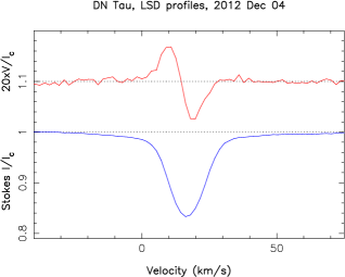
Figure 1: LSD circularly-polarized (Stokes $V$) and unpolarized (Stokes $I$) profiles of DN Tau (top/red, bottom/blue curves respectively) collected on 2012 Dec 04 (cycle 115+1.944). A clear Zeeman signature (with a full amplitude of 0.7%) is detected in the LSD Stokes $V$ profile, in conjunction with the unpolarised line profile. The mean polarization profile is expanded by a factor of 20 and shifted upwards by 1.1 for display purposes.

Least-Squares Deconvolution (LSD, Donati et al., 1997) was applied to all observations. The line list we employed for LSD is computed from an Atlas9 LTE model atmosphere (Kurucz, 1993) featuring $\hbox{$T_{\rm eff}$}=4,000$ K and $\hbox{$\log g$}=3.5$, appropriate for DN Tau (see Sec. 3). As usual, only moderate to strong atomic spectral lines are included in this list (see, e.g., Donati et al., 2010b, for more details).

Altogether, about 9,200 spectral features (with about 35% from Fe i) are used in this process. Expressed in units of the unpolarized continuum level $I_{\rm c}$, the average noise levels of the resulting Stokes $V$ LSD signatures range from 1.9 to 3.6$\times 10^{-4}$ per 1.8 km s^-1 velocity bin (median value 2.3$\times 10^{-4}$) with ESPaDOnS spectra, and about twice as much with NARVAL spectra. Zeeman signatures are detected at all times in LSD profiles and in our two main accretion proxies (see Sec. 4); an example LSD photospheric Zeeman signature (collected during the 2011 run) is shown in Fig. 1 as an illustration.

3 Evolutionary stage of DN Tau

The photospheric temperature of DN Tau (spectral type M0, Cohen & Kuhi, 1979) is often quoted as 3850 K in the literature (e.g., Kenyon & Hartmann, 1995), on account of the reported spectral type. Direct estimates derived from multicolour photometry, lead to similar values (e.g., 3920 K, e.g., Bouvier & Bertout, 1989). Although not mentioned in the corresponding papers, the uncertainties on these estimates are likely to be at least 100 K.

For the present study, we derived a new estimate directly from our spectra of DN Tau thanks to the automatic spectral classification tool especially developed in the context of MaPP, inspired from that of Valenti & Fischer (2005), and already used and discussed in a previous paper of the series (Donati et al., 2012). Not only is this new estimate expected to be more accurate than the older ones, but it should also have the advantage of being homogeneous with measurements obtained with the same tool on all other cTTSs of our sample. Applying it to our spectra of DN Tau, we obtain $\hbox{$T_{\rm eff}$}=3,950\pm 50$ K and $\hbox{$\log g$}=3.7\pm 0.1$, slightly higher though still compatible with older literature estimates. We use this value throughout our paper.

To work out the luminosity of DN Tau, we start from its brightest $V$ magnitude as observed during long-term photometric monitoring, equal to $\hbox{$m_{\rm V}$}=12.1$ (e.g., Artemenko et al., 2012). We first note that the visual extinction that DN Tau suffers is only moderate ($\hbox{$A_{\rm V}$}\simeq 0.5$, Kenyon & Hartmann, 1995) and more or less compensates the limited continuum contribution from accretion veiling (see Sec. 4), at least to a precision of about 0.25 mag - qualitatively consistent with the approximate agreement found between spectroscopic and photometric temperature estimates. Given the temperature of DN Tau, the required bolometric correction to apply is $-1.10$ (Bessell et al., 1998); for a distance to Taurus of 140 pc, the correction to apply (distance modulus) is equal to $-5.73$. Taking finally into account that spots (either always in view, or evenly spread over the surface) are very often present on active stars (and thus on cTTSs as well), typically reducing their luminosity by 20% (even when brightest), we end up for DN Tau with a bolometric magnitude of $5.0\pm 0.25$, i.e., with a logarithmic luminosity (with respect to the Sun) of $-0.1\pm 0.1$. The revised mass that we derive for DN Tau (mostly from $T_{\rm eff}$ and a comparison with evolutionary models of Siess et al., 2000, see Fig. 2) is $\hbox{$M_{\star}$}=0.65\pm 0.05$ ${\rm M}_{\odot}$ (the error bar reflecting mainly the uncertainty on $T_{\rm eff}$); the corresponding radius is $\hbox{$R_{\star}$}=1.9\pm 0.2$ ${\rm R}_{\odot}$, in good agreement with previous estimates (e.g., Appenzeller et al., 2005). The age we infer for DN Tau is $\simeq$2 Myr, clearly indicating that DN Tau is still fully convective (see Fig. 2).

Figure 2: Observed (open square and error bars) location of DN Tau in the HR diagram. The PMS evolutionary tracks and corresponding isochrones (Siess et al., 2000) assume solar metallicity and include convective overshooting. The green line depicts where models predict cTTSs start developing their radiative core as they contract towards the main sequence.

The rotation period of DN Tau has been estimated a number of times, mostly from photometric monitoring (Vrba et al., 1986; Bouvier & Bertout, 1989; Percy et al., 2010; Artemenko et al., 2012); the latest and most accurate of these studies yield a rotation period of 6.32 d (with which we phased all our data, see Sec. 2), in relatively good agreement with previous estimates (ranging from 6.0 to 6.6 d). Recent estimates obtained by monitoring the radial velocity (RV) of DN Tau through cross-correlation of its photospheric spectrum (e.g., Crockett et al., 2012) confirm this periodicity and interpret the observed RV variations as rotational modulation of line profiles induced by the presence of large cool spots at the surface of DN Tau, implying at the same time that the detected period truly relates to the rotation of the star (rather than to some variability in the inner regions of the accretion disc). Our observations fully confirm this view (see Sec. 4).

Given the line-of-sight-projected equatorial rotation velocity $v\sin i$ of DN Tau that we derive (equal to $9\pm 1$ km s^-1, see Sec. 5, in agreement with previous published estimates, e.g., Appenzeller et al., 2005), we obtain (from the radius and period estimated quoted above) that the rotation axis of DN Tau is inclined at $35\pm 10\hbox{${}^{\circ}$}$ to the line of sight, i.e., more or less coincident with that of the accretion disc (e.g., Muzerolle et al., 2003).

4 Spectroscopic variability

We now describe the spectroscopic variability that DN Tau exhibited during our two observing runs, concentrating mostly on photospheric LSD profiles and on a small selection of accretion proxies (i.e., Ca ii infrared triplet / IRT, He i $D_{3}$, H${\alpha}$ and H${\beta}$). In this step, we essentially focus on simple observables that can be derived from these profiles, and in particular on equivalent widths, RVs and longitudinal magnetic fields (i.e., the line-of-sight projected component of the vector field averaged over the visible stellar hemisphere and weighted by brightness inhomogeneities), and look at how they vary with time - both in terms of rotational modulation and intrinsic variability. This basic approach allows in particular to get an intuitive understanding of how the various observables support the existence of the multiple magnetic, brightness and accretion features present at the surface of DN Tau.

4.1 LSD photospheric profiles

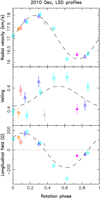
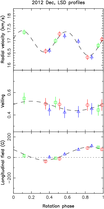
Figure 3: Rotational modulation of the RV (top row), veiling (second row) and longitudinal field (bottom row) derived from the LSD photospheric profiles of DN Tau in late 2010 (left panels) and late 2012 (right panels). Data collected during the successive rotation cycles of each run are shown with different symbols and colors (red open circles, green open squares, dark-blue open triangles, light-blue open five-pointed stars, pink filled triangles, grey open plusses and orange open six-pointed stars respectively indicating rotation cycles 0 to 6). Formal $\pm$1 $\sigma$ error bars (computed from the error bars of the observed spectra) are shown for longitudinal fields, while conservative error bars of $\pm$0.1 km s^-1 and $\pm$0.05 were assumed for RVs and veiling respectively. Fits with sine/cosine waves (and first harmonic, whenever appropriate) are included (and shown as dashed lines) to outline (whenever significant) the amount of variability attributable to rotational modulation. This figure is best viewed in color.

The temporal variability of unpolarized and circularly-polarized LSD profiles of DN Tau is summarised in Fig. 3, showing obvious differences between our two observing runs.

In 2010 Dec (left column of Fig. 3, top panel), RVs of unpolarized LSD profiles exhibit a conspicuous and simple rotational modulation about a mean RV of $\simeq 17.1\pm 0.1$ km s^-1 and with a full amplitude of $\simeq$1.9 km s^-1; this modulation repeats rather well across the 6 rotation cycles, showing only a low level of intrinsic variability. As for most cTTSs studied to date in the MaPP sample, and in agreement with the findings of Crockett et al. (2012), this suggests the presence of a dark spot at the surface of DN Tau, centred at phase 0.50 (i.e., at mid-phase between RV maximum and minimum) and located at high latitudes (given the fairly sinusoidal shape of the RV curve and its small semi-amplitude with respect to $v\sin i$). The period on which RVs fluctuate is $6.33\pm 0.05$ d, in very good agreement with the most recent photometric estimate (Artemenko et al., 2012).

In 2012 Dec (right column of Fig. 3, top panel), RVs of DN Tau show a more complex phase dependence (featuring essentially the second harmonic at half the rotation period) and a twice lower amplitude ($\simeq$1.0 km s^-1) about a mean RV of $\simeq 16.9\pm 0.1$ km s^-1. This clearly indicates that the cool spot present in 2010 Dec on DN Tau significantly changed in both position and size between our two runs, and shows up in 2012 Dec as a complex of two smaller spots / appendages with one appendage on each side of the pole (at phases 0.2 and 0.7 respectively).

At both epochs, DN Tau suffers from a moderate amount of spectral veiling of $\simeq$0.5 (at an average wavelength of 660 nm). The veiling is more variable in 2010 Dec than in 2012 Dec, both in terms of rotational modulation and intrinsic variability. In 2010 Dec, maximum veiling (of $\simeq$0.7) is reached at phase 0.55, suggesting that the accretion region (presumably causing the observed veiling) is close to the cool spot detected from RV variations as in most other cTTSs studied to date; in 2012 Dec, the veiling is more or less constant with phase, suggesting that the accretion region is much closer to the pole than during our first run.

Clear Zeeman signatures are detected at both epochs in the LSD profiles of DN Tau, usually featuring an antisymmetric shape (with respect to the line centre) with a full amplitude of up to 0.8% (of the unpolarized continuum level). Again, rotational modulation (and intrinsic variability) is larger in 2010 Dec, with longitudinal fields (derived from Zeeman signatures with the first moment technique, e.g., Donati et al., 1997) varying from –300 to 200 G (with typical error bars of 12 and 25 G for ESPaDOnS and NARVAL data respectively) on a period (of $6.30\pm 0.15$ d) that agrees well with the estimate of Artemenko et al. (2012).

In 2012 Dec, longitudinal fields are both smaller and mostly positive, varying from –40 to 110 G (with a median error bar of 11 G), but nevertheless show clear modulation on a period (of $6.25\pm 0.10$ d) fully compatible with rotation; from the small amplitude of the rotational modulation, we can guess that the magnetic topology (or at least its most intense low-order component) is better aligned with the rotation axis in our second observing run. As for the veiling, the intrinsic variability of longitudinal fields is smaller in 2012 Dec than in 2010 Dec, suggesting that it likely reflects potential effects of unsteady accretion on Zeeman signatures rather than rapid changes in the large-scale field topology.

4.2 Ca ii IRT emission

Figure 4: RVs (top row), equivalent widths (second row) and longitudinal fields (bottom row) derived from the Ca ii IRT LSD profiles of DN Tau in late 2010 (left panels) and late 2012 (right panels), with symbol/color coding as in Fig. 3. Conservative error bars of $\pm$0.1 and $\pm$1 km s^-1 were assumed for the RVs and equivalent widths of the emission profile. This figure is best viewed in color.

Narrow emission in the core of Ca ii IRT lines is a very convenient proxy of accretion at the surface of low-mass cTTSs, despite tracing simultaneously their non-accreting chromospheres. Being formed closer to the stellar surface and in a more static atmosphere than the He i $D_{3}$ emission line (the usual accretion proxy for cTTSs), the narrow emission cores of the Ca ii IRT lines feature Zeeman signatures that are simple in shape (almost antisymmetric with respect to the line centre) and thus quite easy to model (with no need to account for velocity gradients in the line formation region); moreover, the triplet nature and the IR location of these lines both ensure high-data quality, usually overcompensating the signal dilution from the non-accreting chromospheres.

The accretion proxy we consider here (as in the previous papers of the series) is a LSD-like weighted average of the 3 IRT lines, whose unpolarized profile is corrected by subtracting the underlying (much wider) Lorentzian absorption profile (with a single Lorentzian fit to the far line wings, see, e.g., Donati et al., 2011b, for an illustration). As for photospheric LSD profiles, we investigate how the RV, equivalent width and longitudinal field of this composite emission profile vary with time in the case of DN  Tau, throughout each of our observing runs; the results we obtain are presented graphically on Fig. 4.

We again find that rotational modulation is significantly larger in 2010 Dec (than in 2012 Dec). At this epoch, RVs of the core emission profile are found to vary by up to 3 km s^-1 peak-to-peak, in almost perfect anti-phase with those of LSD profiles and with a period (of $6.22\pm 0.10$ d) in good agreement with that used to phase our data. It suggests that the parent accretion region is centred at phase 0.50 (i.e., at mid-phase between RV minimum and maximum); this is also the phase at which core emission in Ca ii lines (varying from about 9 to 18 km s^-1, or equivalently from 0.027 to 0.050 nm) reaches maximum strength (see Fig. 4, middle left panel) and at which veiling is maximum (see Fig. 3, middle left panel), further confirming our conclusion that the accretion region is more or less coincident with the cool spot traced by photospheric LSD profiles.

In 2012 Dec, the RV curve suggests that the accretion region is centred at phase 0.70 and located closer to the pole (with a peak-to-peak amplitude of only 2 km s^-1). This is fully compatible with the reported emission strengths in the core of the Ca ii IRT lines (exhibiting a much lower level of variability, about a mean of 15 km s^-1 or 0.043 nm, see middle right panel of Fig. 4) and with the more-or-less constant veiling detected at this epoch. We further infer that this accretion region is simpler and less extended than the cool spot traced by photospheric LSD profiles (whose complex shape was readily visible from the corresponding RV curve, see Fig. 3, top right panel).

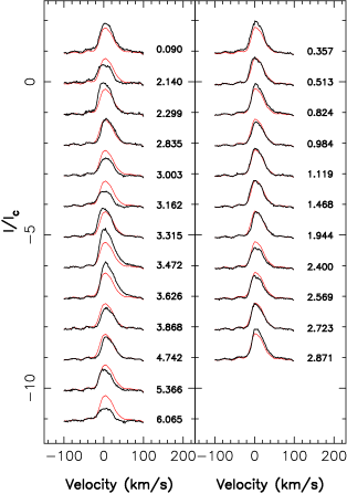
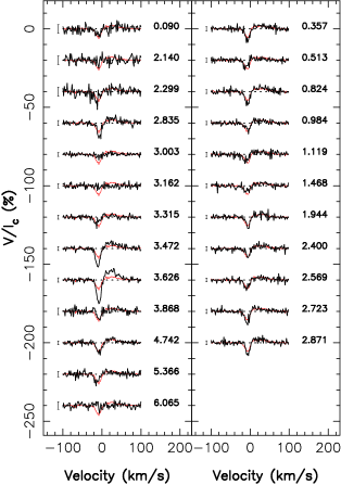
Figure 5: Variations of the unpolarized (Stokes $I$, left panel) and circularly-polarized (Stokes $V$, right panel) profiles of the He i $D_{3}$ emission of DN Tau in 2010 Dec (left columns of both panels) and 2012 Dec (right columns). Clear Zeeman signatures (with full amplitudes of up to 20% in 2009 July) are detected at most epochs; these signatures obviously feature a stronger / narrower blue (negative) lobe and a weaker / wider red (positive) lobe, i.e., have shapes that clearly depart from the usual antisymmetric pattern with respect to the line centre (i.e., with similarly strong / wide blue and red lobes). To emphasize variability, the average profile over each run is shown in red. Rotation cycles (as listed in Table 1) and 3$\sigma$ error bars (for Stokes $V$ profiles only) are shown next to each profile.

We note that at both epochs, Ca ii IRT emission cores of DN Tau are located at an average RV of $\simeq$18 km s^-1, i.e., red-shifted by $\simeq$1 km s^-1 with respect to photospheric lines, typical to the moderately accreting cTTSs observed so far (e.g., Donati et al., 2012)

As for LSD profiles, Zeeman signatures are clearly detected in association with the narrow emission cores of the Ca ii IRT lines, with a full amplitude of up to 10% peak to peak (in units of the unpolarized continuum). The corresponding longitudinal fields range from –140 to 720 G in 2010 and from 200 to 440 G in 2012 (with typical error bars of 40 and 100 G for ESPaDOnS and NARVAL data respectively), i.e., exhibiting both a larger rotational modulation (with a period of $6.19\pm 0.20$ d) and intrinsic variability in the first of our observing runs (see lower panels of Fig. 4). Maximum longitudinal fields are reached around phase 0.60 and 0.70 in 2010 and 2012 respectively, suggesting that the magnetic pole is more or less coincident with the cool polar spot and accretion region already tracked through the other spectral diagnostics (RVs and equivalent widths); the much smaller rotational modulation observed in 2012 also suggests the large-scale field is variable on a timescale of 2 yr, being better aligned with the rotation axis in 2012 than in 2010.

We note that longitudinal fields of DN Tau as derived from LSD profiles and Ca ii emission cores are not systematically of opposite sign, as for other previously studied cTTSs (e.g., TW Hya, Donati et al., 2011b), being even both mainly of the same sign most of the time in 2012 (as for AA Tau, e.g., Donati et al., 2010b); moreover, longitudinal field strengths in LSD profiles are, once averaged over the rotation cycle, much lower than those in Ca ii profiles (by typically a factor of 5 or more) rather than being comparable as for TW Hya. This suggests that the large-scale field at the surface of DN Tau is globally simpler than that of TW Hya, featuring in particular a weaker degree of polarity reversals over the visible hemisphere, and shares similarities with that of AA Tau.

4.3 He i $D_{3}$ emission

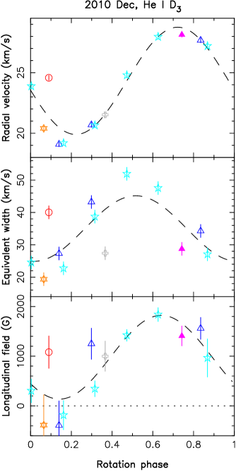
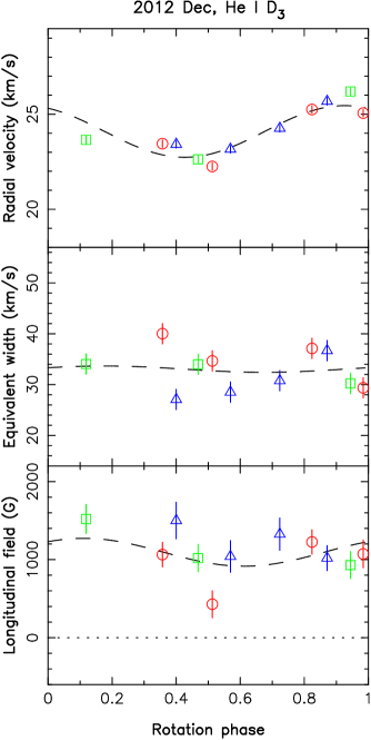
Figure 6: Same as Fig. 4 for the narrow component of the He i $D_{3}$ profiles of DN Tau. Conservative error bars of $\pm$0.2 km s^-1 and $\pm$2 km s^-1 were assumed on the RVs and equivalent widths of the emission profile. This figure is best viewed in color.

The unpolarized and circularly-polarized line profiles of the more conventional accretion proxy often used in cTTSs studies, i.e., the He i $D_{3}$ line, are shown in Fig. 5, as well as their variations with time (with respect to the average) for our two observing runs. They both feature a clearly asymmetric shape, with Stokes $I$ profiles exhibiting a broader red wing (compared to the blue one) and Stokes $V$ profiles showing a blue lobe that is deeper and narrower (than the red one). These asymmetries directly reflect that the He i $D_{3}$ emission of cTTSs is formed in a region featuring strong velocity gradients, presumably probing the postshock zone of the accretion region where the incoming disc plasma is experiencing a strongly decelerating fall towards the stellar surface. We also note that the He i $D_{3}$ line of DN Tau at both epochs only shows a relatively narrow emission component, but no broad emission component as in a number of cTTSs (e.g., TW Hya or GQ Lup Donati et al., 2011b; Donati et al., 2012).

Rotational modulation of the RVs, equivalent widths and longitudinal fields derived from the He i emission, shown in Fig. 6, essentially repeat those inferred from the Ca ii IRT emission core. In 2010, RVs vary more or less sinusoidally with phase, with a period of $6.17\pm 0.10$ d (again compatible with that used to phase the data) and a semi-amplitude of $\simeq$4.5 km s^-1 (about half the $v\sin i$ of DN Tau, see Sec. 5). Assuming as usual that most of the He i emission comes from the accretion region, it indicates that this region is located at phase 0.50 (i.e., at mid time between RV minimum and maximum, fully compatible with results from Ca ii IRT emission) and at latitude $\simeq$60^∘. We also further confirm that RVs vary much less in 2012 (full amplitude of $\simeq$4 km s^-1), indicating that the accretion region has moved much closer to pole, at latitude $\simeq$75^∘ and phase 0.70. In both cases, He i emission occurs at an average RV of $\simeq$24 km s^-1, i.e., red-shifted by $\simeq$7 km s^-1 with respect to average LSD photospheric profiles; as with other cTTSs (e.g., GQ Lup, Donati et al., 2012), this confirms that He i emission is being formed in non-static atmospheric layers, as already evidenced by the strong asymmetries in both Stokes $I$ and $V$ He i profiles (see Fig. 5).

Equivalent widths of He i emission ranges from about 20 to 50 km s^-1 (i.e., 0.040 and 0.100 nm) with an average value of $\simeq$35–40 km s^-1 (i.e., 0.070–0.080 nm, see Fig. 6 mid panels). In 2010, maximum emission is reached at phase 0.50, i.e., when the accretion region (as derived from RV curves) is best viewed from the observer, as expected. In 2012, He i emission is more or less constant with time, in agreement with our finding (from the RV curve) that the accretion region is located much closer to the pole at this epoch. Again, rotational modulation of the equivalent width of He i emission mostly repeats that derived from Ca ii IRT lines.

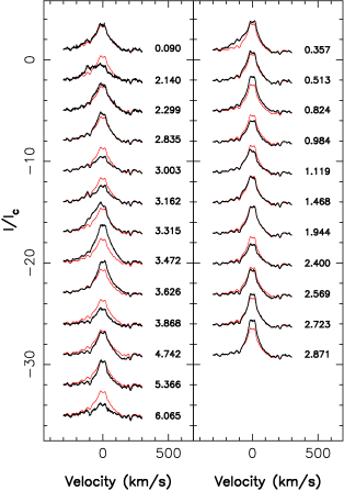
Figure 7: Variations of the H${\alpha}$ (left) and H${\beta}$ (right) lines in the spectrum of DN Tau, in 2010 Dec (left column of both panels) and 2012 Dec (right column). To emphasize variability, the average profile over each run is shown in red. Rotation cycles (as listed in Table 1) are mentioned next to each profile.

Zeeman signatures are detected at most epochs in conjunction with He i emission, indicating the presence of longitudinal fields of up to 1.8 kG in the accretion region of DN Tau (see Fig. 6 bottom panels). Rotational modulation of Zeeman signatures is clear in 2010, with longitudinal fields varying from –0.4 to 1.8 kG (typical error bars of about 200 G for ESPaDOnS data and 400 G for NARVAL data) with a period of $6.10\pm 0.15$ d, in agreement with a magnetic pole significantly offset from the rotation pole. We also note that, as for Ca ii emission, longitudinal fields peak at a slightly later phase (of about 0.60) than equivalent widths, suggesting that the accretion spot is close but not exactly coincident with the magnetic pole. In 2012, longitudinal fields are roughly constant (at about 1.2 kG), the observed temporal evolution being mainly caused by intrinsic variability rather than rotational modulation; this further confirms that the large-scale field of DN Tau is evolving on a timescale of 2 yr, reaching in 2012 a state of near-alignment with the rotation axis.

4.4 Balmer emission

Balmer H${\alpha}$ and H${\beta}$ emission profiles of DN Tau are shown in Fig. 7 at both epochs. For most epochs during our runs, these profiles consist of a central emission peak with an average equivalent width of about 700 and 300 km s^-1 (i.e., 1.5 and 0.50 nm) respectively; additional blue emission (shifted by about 100 km s^-1 with respect to the main central emission) also shows up sporadically in both profiles, though much more conspicuously in H${\alpha}$ than in H${\beta}$ (e.g., at cycles 2.140 and 3.315 in 2010, or at cycle 0.357 in 2012, see Fig. 7).

Looking at variance profiles (not shown here), we obtain that variability occurs in 3 separate regions of these Balmer lines. Most of the variability takes place either in the central emission peak or in the additional blue emission mentioned above, the strongest variability occurring in the central emission peak for H${\beta}$ and in the blue emission component for H${\alpha}$. When most conspicuous (in 2010), the blue H${\alpha}$ emission component is found to vary in a more or less anti-correlated way with the main central emission. This variability, and in particular the one associated with the blue emission component, is apparently not related to rotational modulation, rather discrepant profiles being observed at similar phases of different rotation cycles (e.g., cycles 2.140 and 3.162, or 3.315 and 5.365 in 2010, or 0.357 and 2.400 in 2012).

Variability is also observed, though at a much weaker level, in the red wing of both Balmer profiles (at velocities of 100–200 km s^-1); for contrast reasons, this variability is better observed in H${\beta}$ and shows up as weak absorption transients only visible in a small number of spectra (e.g., at cycle 4.742 in 2010, or 2.569 in 2012). This variability is somewhat reminiscent of the strong absorption features occurring in the red wing of Balmer lines of AA Tau (attributed to the recurring transits of a magnetically-confined accretion funnel over the visible hemisphere of this mainly edge-on prototypical cTTS); however, these red absorption episodes are much weaker in DN Tau (possibly as a result of the low inclination) and possibly less systematic as well (no clear absorption being observed at similar phases of different rotation cycles, e.g., at phase 2.835 in 2010).

     

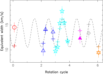
Figure 8: Measured (open symbols) and fitted (pluses) equivalent widths of the Ca ii IRT LSD profiles of DN Tau  in 2010 Dec (left panel) and 2012 Dec (right panel). The model wave (dashed line) providing the best (sine+cosine) fit to the data presumably traces rotational modulation (with a period of 6.32 d), while the deviation from the fit illustrates the level of intrinsic variability. The open symbols are defined as described in Fig. 3. This figure is best viewed in color.

4.5 Mass-accretion rate

From the emission strength of the various accretion proxies mentioned above, we can derive an estimate of the mass accretion rate using the same method as that outlined in the previous papers of the series (e.g., Donati et al., 2012). Approximating the stellar continuum by a Planck function at temperature 3,950 K, we derive, from the Ca ii IRT, He i, H${\beta}$ and H${\alpha}$ equivalent widths reported above (respectively equal to 0.045, 0.075, 0.50 and 1.5 nm), logarithmic line fluxes (in units of the solar luminosity ${\rm L}_{\odot}$) of –3.5, –4.2, –4.9 and –5.1. Using the empirical calibrations of Fang et al. (2009), these line fluxes translate into logarithmic accretion luminosities of –2.2, –2.4, –1.7 and –2.3 respectively (again in units of ${\rm L}_{\odot}$). From this we infer that the average logarithmic mass accretion rate at the surface of DN Tau (in units of ${\rm M}_{\odot}$ yr^-1) is $-9.1\pm 0.3$ at both epochs (with estimates derived from individual proxies agreeing all with this value within the quoted error bar). Very similar results are obtained (logarithmic mass accretion rate of $-9.2\pm 0.3$ ${\rm M}_{\odot}$ yr^-1) when using the newer empirical calibrations of Rigliaco et al. (2012). Our estimate is also in rough agreement with the older one of Gullbring et al. (1998), equal to $-8.5$ ${\rm M}_{\odot}$ yr^-1, based on measurements of the UV continuum excess presumably produced by accretion - especially if we allow for likely systematic differences between both types of measurements (see, e.g., Rigliaco et al., 2012), as well as for potential long-term variations of the accretion rate between our observations and those used by Gullbring et al. (1998).

An independent (though much less accurate) estimate can also be obtained from the width of H${\alpha}$ (e.g., Natta et al., 2004). Given the full width at 10% height of $300\pm 20$ km s^-1 of the average H${\alpha}$ profile of DN Tau, we infer a logarithmic mass accretion rate of $-10.0\pm 0.6$, smaller and marginally compatible with our previous estimate. However, as already stressed by Cieza et al. (2010), the precision of this measurement technique depends in an unclear way on the overall shape of H${\alpha}$ (and of its variations with time), rendering this accretion proxy a relatively poor quantitative indicator in practice; for this reason, we disregard this latter estimate and only consider our former (and main) measurement of the accretion rate in the remaining sections of our paper.

5 Magnetic modelling

After this qualitative overview and preliminary analysis of our data sets, we now propose a more quantitative and unbiased modeling of the photospheric LSD and Ca ii IRT unpolarized and circularly-polarized profiles in terms of maps of the large-scale magnetic topology, and of distributions of photospheric cool spots and of chromospheric accretion regions, at the surface of DN Tau. The software tool we are using in this aim is a dedicated stellar-surface tomographic-imaging package based on the principles of maximum-entropy image reconstruction and on the main assumption that the observed variability is mainly caused by rotational modulation; our code was adapted to the specific needs of MaPP observations (Donati et al., 2010b) and extensively tested on a number of previous data sets (e.g., Donati et al., 2011a; Donati et al., 2012) including close binary stars (Donati et al., 2011c).

More specifically, the code is set up to invert (both automatically and simultaneously) time series of Stokes $I$ and $V$ LSD and Ca ii profiles into magnetic, brightness and accretion maps of the observed protostar. The reader is referred to Donati et al. (2010b) for more details on the imaging method.

5.1 Application to DN Tau

We start the process by applying to our data sets the usual filtering techniques, designed for retaining rotational modulation while discarding intrinsic variability (see, e.g., Donati et al., 2010b, 2012, for more information). The effect of this process on Ca ii profiles is illustrated in Fig. 8 in the particular case of DN Tau. In practice, this filtering has little impact on the reconstructed maps, and essentially allows us to ease the convergence of the iterative optimization algorithm on which the imaging code is based.

The local Stokes $I$ and $V$ profiles are synthesized using Unno-Rachkovsky’s solution to the equations of polarized radiative transfer in a Milne-Eddington model atmosphere, known to provide a reliable description (including magneto-optical effects) of how shapes of line profiles are distorted in the presence of magnetic fields (e.g., Landi degl’Innocenti & Landolfi, 2004). The main local line parameters used for DN Tau are again very similar to those used in our previous studies. For the average photospheric LSD profile, the wavelength, Doppler width, unveiled equivalent width and Landé factor are respectively set to 660 nm, 1.9 km s^-1, 4.2 km s^-1 and 1.2; for the quiet Ca ii emission profile, they are respectively set to 850 nm, 7 km s^-1, 10 km s^-1 and 1.0. Finally, we assume that Ca ii emission is locally enhanced in accretion regions (with respect to quiet chromospheric regions) by a factor $\epsilon=10$, as in all previous studies.

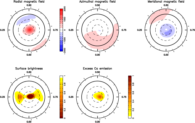
Figure 9: Maps of the radial, azimuthal and meridional components of the magnetic field $\bf B$ (first and third rows, left to right panels respectively), photospheric brightness and excess Ca ii IRT emission (second and fourth rows, first and second panels respectively) at the surface of DN Tau, in 2010 Dec (top two rows) and 2012 Dec (bottom two rows). Magnetic fluxes are labelled in G; local photospheric brightness (normalized to that of the quiet photosphere) varies from 1 (no spot) to 0 (no light); local excess Ca ii emission varies from 0 (no excess emission) to 1 (excess emission covering 100% of the local grid cell, assuming an intrinsic excess emission of 10$\times$ the quiet chromospheric emission). In all panels, the star is shown in flattened polar projection down to latitudes of $-30\hbox{${}^{\circ}$}$, with the equator depicted as a bold circle and parallels as dashed circles. Radial ticks around each plot indicate phases of observations. This figure is best viewed in color.

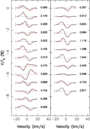
Figure 10: Maximum-entropy fit (thin red line) to the observed (thick black line) Stokes $I$ and Stokes $V$ LSD photospheric profiles (top panels) and Ca ii IRT profiles (bottom panels) of DN Tau. In each panel, the left and right columns correspond to the 2010 Dec and 2012 Dec data respectively. The light-blue curve in the bottom left panel shows the (constant) contribution of the quiet chromosphere to the Stokes $I$ Ca ii profiles. Rotational cycles and 3$\sigma$ error bars (for Stokes $V$ profiles) are also shown next to each profile.

The reconstructed magnetic, brightness and accretion maps of DN Tau are shown in Fig. 9 for both epochs, with the corresponding fits to the data shown in Fig. 10. Once again, we assume that the magnetic topology of DN Tau is antisymmetric with respect to the centre of the star; the spherical harmonic (SH) expansions describing the reconstructed field is limited to terms with $\ell\leq 7$, which is found to be adequate when $\hbox{$v\sin i$}<10$ km s^-1.

Error bars on Zeeman signatures were artificially expanded by a factor of 1.5 (in 2010) to 2 (in 2012), both for LSD profiles and for Ca ii emission, to compensate for the level of intrinsic variability specific to the Stokes $V$ data, obvious from the lower panels of Figs. 3 and 4 (where the observed dispersion on longitudinal fields is larger than formal error bars) and not removed by our filtering process (correcting irregular changes in line equivalent widths only). The fits we finally obtain correspond to a reduced chi-square $\chi^{2}_{\rm r}$ equal to 1, starting from initial values of about 9 and 16 in 2010 and 2012 respectively (for a null magnetic field and unspotted brightness and accretion maps, and with scaled-up error bars on Zeeman signatures).

As part of the imaging process, we obtain new, more accurate estimates for a number of parameters of DN Tau. We find in particular that the average RV of DN Tau is $17.0\pm 0.1$ km s^-1 at both epochs and that $v\sin i$ is equal to $9\pm 1$ km s^-1, compatible with previous literature estimates (e.g., Appenzeller et al., 2005). We also find that Zeeman signatures are best fitted for values of the local filling factor (describing the relative proportion of magnetic areas at any given cell of the stellar surface, see Donati et al., 2010b) equal to $\psi\simeq$1, significantly larger than that derived for most cTTSs analysed to date (for which $\psi\simeq 0.4$, e.g., Donati et al., 2011a).

5.2 Modelling results

As clear from Fig. 9, the large-scale fields reconstructed for DN Tau at both epochs are mainly axisymmetric. Their main feature is a region of positive radial field located at a latitude of 60^∘ and phase 0.50 in 2010 and almost exactly on the pole in 2012; the magnetic flux in this region reaches about 1.8 kG in 2010 and 1.3 kG in 2012, in good agreement with the maximum longitudinal field values probed by the He i accretion proxy (see Fig. 6, lower panels). Both maps include low-latitude arcs of negative radial field resembling those found on previously studied cTTSs (like GQ Lup, Donati et al., 2012) but with a lower contrast, i.e., a weaker flux relative to that of the main radial field region; similarly, both maps also feature a high-latitude ring of mostly negative (i.e., equatorward) meridional field surrounding the main magnetic pole.

The reconstructed field is mostly poloidal, the toroidal component storing no more than 10–15% of the overall magnetic energy. The poloidal component is mostly axisymmetric in 2012, with more than 80% of the magnetic energy concentrating in SH modes with $m<\ell/2$ ($\ell$ and $m$ denoting respectively the degrees and orders of the modes); this fraction drops down to only $\simeq$50% in 2010 as a result of the significant tilt of the large-scale field (with respect to the rotation axis).

We find that the octupole field dominates the large-scale surface field at both epochs, concentrating about 45 and 60% of the poloidal magnetic energy in 2010 and 2012 respectively, whereas the dipole field only stores 35 and 20% of the energy at these 2 epochs; their corresponding strengths at the surface of DN Tau are respectively equal to 780 and 600 G in 2010 and 2012 for the octupole component, and to 530 and 300 G for the dipole component, implying octupole to dipole intensity ratios of 1.5 and 2.0 at both epochs. This confirms in particular that the large-scale field of DN Tau significantly weakened between 2010 and 2012, as guessed from the long-term evolution of the longitudinal field curves (see Sec. 4). This weakening apparently affects the dipole component more than the octupole one; we however caution that the octupole to dipole intensity ratio, although well constrained in 2010 and rather insensitive to minor inversion parameters (like for instance the relative $\chi^{2}$ level to which the data are fitted or the relative weight assigned to the different reconstructed image quantities in the entropy functional), is more uncertain in 2012 with potential values varying from 1.5 to 2.5. We thus conclude that the weakening of the overall field is clear, but that the corresponding topological change to a more octupolar configuration of the field is only likely.

We also find that the dipole and octupole components are more or less parallel to each other, with respective tilts to the rotation axis of about 25–30^∘ for the dipole (towards phase 0.2 and 0.9 in 2010 and 2012 respectively), and 30 and 0^∘ for the octupole (towards phase 0.5 in 2010). In particular, the change in the tilt of the octupole component (to the rotation axis) between 2010 and 2012 is clear and well constrained by the observations; the tilts and phase of the dipole component is less secure, and likely not accurate to better than 10^∘ and 0.10 cycle respectively.

The surface brightness distributions that we reconstruct for DN Tau in 2010 and 2012 both include a dark spot close to the pole, but nevertheless feature a number of clear differences. In 2010, the polar spot is essentially monolithic, significantly off-centred from the pole (by about 30^∘ towards phase 0.50) and covering $\simeq$6% of the overall stellar surface. In 2012, the surface brightness distribution of DN Tau is more complex, as readily visible from the RV curve derived from LSD profiles (see top right panel of Fig. 3). It includes not only one cool polar spot almost centred on the pole (with a low-contrast appendage towards lower latitudes at phase 0.70), but also a second cool region located at intermediate latitudes and centred at phase 0.25; the overall filling factor associated with this brightness distribution is now only $\simeq$4.5% (including the contribution of both cool features), i.e., significantly smaller than that derived from our 2010 observations. This clearly demonstrates that the brightness distribution of DN Tau significantly evolved between 2010 and 2012; moreover, since the main cool polar spot overlaps almost perfectly with the main radial field magnetic region at both epochs, it suggests that the temporal evolution of the brightness distribution mostly reflects the underlying change in the large-scale magnetic topology.

The overlap of dark spots and magnetic regions also explains a posteriori why the most intense fields reconstructed at the surface of DN Tau are not detected through LSD photospheric profiles (see longitudinal field curves at both epochs, bottom panels of Fig. 3). Given their low relative brightness, dark spots emit few photons (compared to the surrounding unspotted photosphere) and therefore few circularly polarized photons from the magnetic regions that they harbor, even for strong magnetic fields; Stokes $V$ Zeeman signatures from the darkest magnetic regions imaged at the surface of DN Tau are thus too weak to allow retrieving the kG field regions they host from LSD profiles alone, even when brightness distributions are reconstructed simultaneously with magnetic maps. Photospheric lines are however crucial for reconstructing the magnetic topology at equatorial and intermediate latitudes - a key asset for unravelling the respective contribution of the dipolar and octupolar components in the mutipolar field expansion.

Maps of excess Ca ii emission show a clear accretion region located close to the pole, at latitude $\simeq$60^∘ and phase 0.55 in 2010, and latitude $\simeq$75^∘ and phase 0.75 in 2012. In both cases, this accretion region is located within the darkest spot traced by photospheric LSD profiles and covers about 1.5% of the overall stellar surface. Zeeman signatures from accretion proxies thus ideally complement those from photospheric LSD profiles, allowing us to derive a well-constrained description of the large-scale field by providing the missing piece of the puzzle (the kG fields within the dark polar spot). The latitudinal shift of the accretion region between 2010 and 2012 is readily visible from the rotational modulation of Ca ii and He i emission profiles (much smaller in 2012 than in 2010, see Figs. 4 and 6) and further supports our conclusion that the orientation of the overall magnetic topology evolved between the two epochs, getting better aligned with the rotation axis in 2012. We also note that the accretion region features a low-contrast crescent-shaped appendage in 2010, while it is more circular and compact during our second observing run (2012).

6 Summary & discussion

Our paper presents dual-epoch spectropolarimetric observations of the cTTS DN Tau aimed at unveiling the large-scale magnetic topology present at the surface of the protostar, at looking for potential long-term temporal variations of this magnetic topology, and at investigating how it impacts accretion from the inner regions of the accretion disc to the stellar surface. Being part of the MaPP Large program with ESPaDOnS at CFHT, this analysis comes as a follow-up of all similar studies published so far on this subject and brings further information on how large-scale fields of cTTSs depend on fundamental parameters such as mass and age. More specifically, the current paper focusses on the second lowest mass star of our sample, thus complementing the surprising results obtained on the only very-low-mass cTTS observed to date (i.e., the 0.35 ${\rm M}_{\odot}$ fully-convective protostar V2247 Oph, Donati et al., 2010a) and to get further clues on what large-scale fields of cTTSs look like in the very-low-mass regime where rotational evolution is different (see Sec.1).

Our spectropolarimetric data of DN Tau were collected in 2010 Dec and 2012 Dec with ESPaDOnS at CFHT, and first allowed us to derive a new estimate of the photospheric temperature (in reasonable agreement with previous reports in the literature) and to confirm that DN Tau is a $\simeq$2 Myr-old fully-convective $0.65\pm 0.05$ ${\rm M}_{\odot}$ star. Clear circularly-polarized Zeeman signatures are detected at most epochs in both LSD profiles of photospheric lines and in the narrow emission features probing ongoing accretion in chromospheric layers; the corresponding longitudinal fields range from –0.3 to 0.2 kG in photospheric lines, from –0.1 to 0.7 kG in the emission core of Ca ii lines, and from –0.4 to 1.8 kG in the narrow emission profile of He i $D_{3}$ lines. Temporal variability of both Zeeman signatures and unpolarized line profiles include a significant level of rotational modulation (see Sec. 4), with a period fully compatible with the most recent literature estimate (i.e., 6.32 d, Artemenko et al., 2012); this confirms in particular that the rotation axis of DN Tau is inclined at $\simeq$35^∘ to the line of sight.

Worth noting is that longitudinal fields of DN Tau as derived from LSD profiles and accretion proxies are not systematically of opposite signs (as was the case for, e.g., TW Hya, Donati et al., 2011b), and are even most of the time of the same sign in 2012 Dec (as was the case for AA Tau, Donati et al., 2010b); moreover, longitudinal field strengths in LSD profiles are, once averaged over the rotation cycle, much lower than those in Ca ii lines, by typically a factor of 5, rather than being comparable (as for TW Hya). This qualitatively suggests that the underlying large-scale magnetic topology of DN Tau is significantly simpler than that of TW Hya - a conclusion confirmed by the subsequent detailed profile modeling. We also report in this paper clear evidence that the large-scale field of DN Tau is evolving with time between our two observing campaigns, both in intensity and orientation, making DN Tau similar to V2129 Oph and GQ Lup in this respect (Donati et al., 2011a; Donati et al., 2012).

Thanks to our dedicated tomographic imaging code (tested and optimized for the specific needs of our MaPP observations), we derived, from simultaneous fits to our sets of unpolarized and circularly-polarized LSD photospheric profiles and accretion proxies, maps of the large-scale field of DN Tau at both observing epochs, along with surface distributions of its photospheric dark spots and its accretion regions. We find that DN Tau hosts a mostly poloidal large-scale field, largely axisymmetric with respect to the rotation axis and with a polar field strength reaching 1.8 and 1.3 kG at both epochs respectively. The octupolar component of the large-scale field (of polar strength 780 and 600 G in 2010 and 2012 respectively) is larger than the dipole component (530 and 300 G in 2010 and 2012) by a factor of 1.5 (in 2010) to 2.0 (in 2012); it implies that the overall topology of DN Tau remains rather simple, featuring in particular no high-contrast polarity reversals over the visible hemisphere. This makes DN Tau the cTTS harbouring the simplest magnetic topology of all MaPP stars observed to date, after that of AA Tau (whose large-scale field is dominated by a dipole at least $\simeq$4 times stronger than the octupole component). The orientation of the octupole component (roughly parallel to the dipole component) is clearly changing with time; tilted at $\simeq$30^∘ in 2010, it is almost aligned with the rotation axis in 2012, further demonstrating the genuine variability of the large-scale fields of cTTSs on timescales of years.

Figure 11: Basic properties of the large-scale magnetic topologies of cTTSs, as a function of their locations in the HR diagram. Symbol size indicates relative magnetic intensities, symbol color illustrates field configurations (red to blue for purely poloidal to purely toroidal fields), and symbol shape depicts the degree of axisymmetry of the poloidal field component (decagon and stars for purely axisymmetric and purely nonaxisymmetric poloidal fields, respectively). The large-scale field of DN Tau is weaker than that of AA Tau and BP Tau, but still mainly poloidal and largely axisymmetric (the non-decagonal shape of the symbol being due to the 30^∘ tilt of the octupole field in 2010). The PMS evolutionary tracks and corresponding isochrones (Siess et al., 2000) assume solar metallicity and include convective overshooting. The full lines depict where models predict cTTSs start developing their radiative core (green line) and when their convective envelope is thinner than 0.5 $R_{\star}$(red line), as they contract towards the main sequence. This figure is best viewed in color.

The large-scale field we recover for DN Tau features both similarities and differences with those of the other cTTSs observed in the MaPP framework (see Fig. 11). It is largely poloidal, with an octupole to dipole intensity ratio smaller than 2, like other fully-convective cTTSs located nearby in the HR diagram (namely AA Tau and BP Tau); it is however quite different from that of the very-low-mass cTTS V2247 Oph (the closest fully-convective neighbour of DN Tau on the very-low-mass side of the MaPP sample) whose large-scale field includes a significant toroidal component and a mostly non-axisymmetric poloidal component. However, the large-scale field of DN Tau is significantly weaker than that of its higher mass neighbours AA Tau and BP Tau and more comparable (in strength) to that of V2247 Oph despite the difference in topology. We think that these discrepancies are unlikely attributable to temporal variations of the large-scale fields resulting from non-stationary dynamos - usually much smaller in amplitude than this interpretation would require; we rather speculate that these differences illustrate the expected progressive topological transition between low-mass and very-low-mass fully-convective cTTSs, similar to that observed between mid-M and late-M main-sequence dwarfs (e.g., Morin et al., 2008, 2010). In both cases, our observations bring yet further support on the fact that large-scale fields of cTTSs are produced through non-stationary dynamo processes.

Gregory et al. (2012) reasoned that, as with late-M-dwarfs, the lowest mass cTTSs may host a variety of field topologies, some being significantly more complex than what is found for the more massive fully-convective stars such as AA Tau (Donati et al., 2010b). They argued that a bistable dynamo regime would exist somewhere between 0.2 ${\rm M}_{\odot}$ as a lower limit (the mass below which bistable dynamo behaviour has been observed for main sequence M-dwarfs, Morin et al., 2010) and 60% of the fully-convective limit at any given PMS age as an upper limit (as fully-convective stars are found below 0.35 ${\rm M}_{\odot}$ on the main sequence, and 0.2 ${\rm M}_{\odot}$ is $\simeq$60% of this mass). As we go to successively older ages, the mass below which fully-convective cTTSs are found decreases (see Fig. 11 and equation B1 in Gregory et al., 2012). At the age of DN Tau, $\simeq$1.7 Myr, the fully convective limit is $\simeq$1.2 ${\rm M}_{\odot}$. With a mass of 0.65 ${\rm M}_{\odot}$, DN Tau therefore lies below the upper limit where Gregory et al. (2012) argued that bistable dynamo behaviour may be found. This may explain the weaker field of DN Tau relative to the more massive fully convective stars AA Tau and BP Tau.

We report as well the presence of a dark photospheric region overlapping the main magnetic pole of DN Tau at both epochs, as in all other fully- or mainly-convective cTTSs with masses larger than 0.6 ${\rm M}_{\odot}$ observed so far with MaPP. Similarly, DN Tau also features an accretion region at chromospheric level, located close to the magnetic pole and within the dark photospheric spot, strongly suggesting that accretion from the inner disc regions is occurring mostly poleward in DN Tau as well. We note that the accretion region features a crescent shape in 2010, i.e., when the octupole to dipole intensity ratio is smallest, while it shows a more circular shape in 2012, i.e., when the octupole to dipole intensity ratio is largest (than in 2010); this behaviour is in qualitative agreement with what we expect for the shape of accretion spots from theoretical simulations of magnetospheric accretion (e.g., Romanova et al., 2004b, 2011).

Given the logarithmic mass accretion rate (of $-9.1\pm 0.3$ in ${\rm M}_{\odot}$ yr^-1) that we infer from emission fluxes of conventional accretion proxies, we obtain that the large-scale field of DN Tau should be able to disrupt the accretion disc up to a radius of $\hbox{$r_{\rm mag}$}\simeq 5.9$ $R_{\star}$ (0.052 au) in 2010 and $\simeq 4.3$ $R_{\star}$ (0.038 au) in 2012 (assuming an average dipole strength of 0.53 and 0.30 kG in 2010 and 2012 respectively, and using the analytical formula of Bessolaz et al., 2008). When $r_{\rm mag}$ is compared to the corotation radius $\hbox{$r_{\rm cor}$}\simeq 6.6$ $R_{\star}$ (or 0.058 au), at which the Keplerian period equals the stellar rotation period, we find that $\hbox{$r_{\rm mag}$}/\hbox{$r_{\rm cor}$}$ is equal to $\simeq 0.90$ and $\simeq 0.65$ in 2010 and 2012 respectively. We caution that this estimate of $\hbox{$r_{\rm mag}$}/\hbox{$r_{\rm cor}$}$ (assuming a sonic Mach number at disc mid-plane of $m_{\rm s}\simeq$1, see Bessolaz et al., 2008) is likely an upper limit only, numerical simulations suggesting a potential overestimate of $\simeq$20% (Bessolaz et al., 2008).

Whereas spin-down effects caused by star/disc magnetic coupling can be effective and partly counteract the accretion torque even when $\hbox{$r_{\rm mag}$}/\hbox{$r_{\rm cor}$}\simeq$ 0.5–0.8, recent numerical simulations suggest that they can only overcome both the accretion and stellar contraction torques for values of $\hbox{$r_{\rm mag}$}/\hbox{$r_{\rm cor}$}\simeq$ 0.8–1, at which outflows are generated in the form of magnetospheric ejections through a propeller-like mechanism (e.g., Romanova et al., 2004a; Zanni & Ferreira, 2013). Accretion-powered stellar winds (Matt & Pudritz, 2005, 2008) are also unlikely to succeed at spinning down DN Tau; the wind spin-down torque would indeed require the mass ejection rate of DN Tau to be several times larger than the mass accretion rate we determined - obviously not compatible with the fact that DN Tau is not in a propeller-like regime (where most of disc material is ejected and only a small fraction gets accreted). This suggests that DN Tau already entered a phase of spin-up, and potentially explains why it is rotating slightly faster (with a period of 6.32 d) than prototypical slowly-rotating cTTSs like AA Tau.

Conversely to the case of non-fully-convective cTTSs like TW Hya or V2129 Oph, the reason of the spin-up of DN Tau (and of the correspondingly weaker dipole component) is not attributable to a recent change in the internal stellar structure. We rather speculate that this is caused by a different regime of dynamo processes in very-low-mass stars, having much harder times at producing strong, aligned dipolar fields, with DN Tau and V2247 Oph providing examples of a smooth progressive transition to this new dynamo regime; this could qualitatively explain at the same time the specific rotational evolution that very-low-mass protostars are subject to. More spectropolarimetric observations like those reported here, especially in the low-mass, fully-convective region of the HR diagram, are required to confirm our speculations. In particular, SPIRou, the nIR spectropolarimeter / high-precision velocimeter presently designed as a next generation instrument for CFHT, should be particularly efficient at exploring this region of the HR diagram to investigate in more details bistable dynamos of cTTSs.

References

- Adams & Gregory (2012) Adams F. C., Gregory S. G., 2012, ApJ, 744, 55
- André et al. (2009) André P., Basu S., Inutsuka S., 2009, The formation and evolution of prestellar cores. Cambridge University Press, pp 254
- Appenzeller et al. (2005) Appenzeller I., Bertout C., Stahl O., 2005, A&A, 434, 1005
- Artemenko et al. (2012) Artemenko S. A., Grankin K. N., Petrov P. P., 2012, Astronomy Letters, 38, 783
- Bessell et al. (1998) Bessell M. S., Castelli F., Plez B., 1998, A&A, 333, 231
- Bessolaz et al. (2008) Bessolaz N., Zanni C., Ferreira J., Keppens R., Bouvier J., 2008, A&A, 478, 155
- Bouvier et al. (2007) Bouvier J., Alencar S. H. P., Harries T. J., Johns-Krull C. M., Romanova M. M., 2007, in Reipurth B., Jewitt D., Keil K., eds, Protostars and Planets V Magnetospheric Accretion in Classical T Tauri Stars. pp 479–494
- Bouvier & Bertout (1989) Bouvier J., Bertout C., 1989, A&A, 211, 99
- Cieza et al. (2010) Cieza L. A., Schreiber M. R., Romero G. A., Mora M. D., Merin B., Swift J. J., Orellana M., Williams J. P., Harvey P. M., Evans N. J., 2010, ApJ, 712, 925
- Cohen & Kuhi (1979) Cohen M., Kuhi L. V., 1979, ApJS, 41, 743
- Crockett et al. (2012) Crockett C. J., Mahmud N. I., Prato L., Johns-Krull C. M., Jaffe D. T., Hartigan P. M., Beichman C. A., 2012, ApJ, 761, 164
- Donati et al. (2011a) Donati J., Bouvier J., Walter F. M., Gregory S. G., Skelly M. B., Hussain G. A. J., Flaccomio E., Argiroffi C., Grankin K. N., Jardine M. M., Ménard F., Dougados C., Romanova M. M., 2011a, MNRAS, 412, 2454
- Donati & Landstreet (2009) Donati J., Landstreet J. D., 2009, ARA&A, 47, 333
- Donati et al. (2010b) Donati J., Skelly M. B., Bouvier J., Gregory S. G., Grankin K. N., Jardine M. M., Hussain G. A. J., Ménard F., Dougados C., Unruh Y., Mohanty S., Aurière M., Morin J., Farès R., 2010b, MNRAS, 409, 1347
- Donati et al. (2010a) Donati J., Skelly M. B., Bouvier J., Jardine M. M., Gregory S. G., Morin J., Hussain G. A. J., Dougados C., Ménard F., Unruh Y., 2010a, MNRAS, 402, 1426
- Donati (2003) Donati J.-F., 2003, in Trujillo-Bueno J., Sanchez Almeida J., eds, Astronomical Society of the Pacific Conference Series Vol. 307 of Astronomical Society of the Pacific Conference Series, ESPaDOnS: An Echelle SpectroPolarimetric Device for the Observation of Stars at CFHT. pp 41
- Donati et al. (2011b) Donati J.-F., Gregory S. G., Alencar S. H. P., Bouvier J., Hussain G., Skelly M., Dougados C., Jardine M. M., Ménard F., Romanova M. M., Unruh Y. C., 2011b, MNRAS, 417, 472
- Donati et al. (2012) Donati J.-F., Gregory S. G., Alencar S. H. P., Hussain G., Bouvier J., Dougados C., Jardine M. M., Ménard F., Romanova M. M., 2012, MNRAS, 425, 2948
- Donati et al. (2011c) Donati J.-F., Gregory S. G., Montmerle T., Maggio A., Argiroffi C., Sacco G., Hussain G., Kastner J., Alencar S. H. P., Audard M., Bouvier J., Damiani F., Güdel M., Huenemoerder D., Wade G. A., 2011c, MNRAS, 417, 1747
- Donati et al. (2007) Donati J.-F., Jardine M. M., Gregory S. G., Petit P., Bouvier J., Dougados C., Ménard F., Cameron A. C., Harries T. J., Jeffers S. V., Paletou F., 2007, MNRAS, 380, 1297
- Donati et al. (2008) Donati J.-F., Jardine M. M., Gregory S. G., Petit P., Paletou F., Bouvier J., Dougados C., Ménard F., Cameron A. C., Harries T. J., Hussain G. A. J., Unruh Y., Morin J., Marsden S. C., Manset N., Aurière M., Catala C., Alecian E., 2008, MNRAS, 386, 1234
- Donati et al. (1997) Donati J.-F., Semel M., Carter B. D., Rees D. E., Collier Cameron A., 1997, MNRAS, 291, 658
- Fang et al. (2009) Fang M., van Boekel R., Wang W., Carmona A., Sicilia-Aguilar A., Henning T., 2009, A&A, 504, 461
- Gregory et al. (2012) Gregory S. G., Donati J.-F., Morin J., Hussain G. A. J., Mayne N. J., Hillenbrand L. A., Jardine M., 2012, ApJ, 755, 97
- Gullbring et al. (1998) Gullbring E., Hartmann L., Briceno C., Calvet N., 1998, ApJ, 492, 323
- Irwin & Bouvier (2009) Irwin J., Bouvier J., 2009, in Mamajek E. E., Soderblom D. R., Wyse R. F. G., eds, IAU Symposium Vol. 258 of IAU Symposium, The rotational evolution of low-mass stars. pp 363–374
- Johns-Krull (2007) Johns-Krull C. M., 2007, ApJ, 664, 975
- Johns-Krull et al. (1999) Johns-Krull C. M., Valenti J. A., Koresko C., 1999, ApJ, 516, 900
- Kenyon & Hartmann (1995) Kenyon S. J., Hartmann L., 1995, ApJS, 101, 117
- Kurucz (1993) Kurucz R., 1993, CDROM # 13 (ATLAS9 atmospheric models) and # 18 (ATLAS9 and SYNTHE routines, spectral line database). Smithsonian Astrophysical Observatory, Washington D.C.
- Landi degl’Innocenti & Landolfi (2004) Landi degl’Innocenti E., Landolfi M., 2004, Polarisation in spectral lines. Dordrecht/Boston/London: Kluwer Academic Publishers
- Matt & Pudritz (2005) Matt S., Pudritz R. E., 2005, ApJL, 632, L135
- Matt & Pudritz (2008) Matt S., Pudritz R. E., 2008, ApJ, 681, 391
- Matt et al. (2012) Matt S. P., Pinzón G., Greene T. P., Pudritz R. E., 2012, ApJ, 745, 101
- Mohanty & Shu (2008) Mohanty S., Shu F. H., 2008, ApJ, 687, 1323
- Morin et al. (2010) Morin J., Donati J., Petit P., Delfosse X., Forveille T., Jardine M. M., 2010, MNRAS, 407, 2269
- Morin et al. (2008) Morin J., Donati J.-F., Petit P., Delfosse X., Forveille T., Albert L., Aurière M., Cabanac R., Dintrans B., Fares R., Gastine T., Jardine M. M., Lignières F., Paletou F., Ramirez Velez J. C., Théado S., 2008, MNRAS, 390, 567
- Muzerolle et al. (2003) Muzerolle J., Calvet N., Hartmann L., D’Alessio P., 2003, ApJL, 597, L149
- Natta et al. (2004) Natta A., Testi L., Muzerolle J., Randich S., Comerón F., Persi P., 2004, A&A, 424, 603
- Percy et al. (2010) Percy J. R., Grynko S., Seneviratne R., Herbst W., 2010, PASP, 122, 753
- Rigliaco et al. (2012) Rigliaco E., Natta A., Testi L., Randich S., Alcalà J. M., Covino E., Stelzer B., 2012, A&A, 548, A56
- Romanova et al. (2011) Romanova M. M., Long M., Lamb F. K., Kulkarni A. K., Donati J., 2011, MNRAS, 411, 915
- Romanova et al. (2004a) Romanova M. M., Ustyugova G. V., Koldoba A. V., Lovelace R. V. E., 2004a, ApJL, 616, L151
- Romanova et al. (2004b) Romanova M. M., Ustyugova G. V., Koldoba A. V., Lovelace R. V. E., 2004b, ApJ, 610, 920
- Siess et al. (2000) Siess L., Dufour E., Forestini M., 2000, A&A, 358, 593
- Valenti & Fischer (2005) Valenti J. A., Fischer D. A., 2005, ApJS, 159, 141
- Vrba et al. (1986) Vrba F. J., Rydgren A. E., Chugainov P. F., Shakovskaia N. I., Zak D. S., 1986, ApJ, 306, 199
- Zanni & Ferreira (2013) Zanni C., Ferreira J., 2013, A&A, 550, A99