TMD Evolution: Matching SIDIS to Drell-Yan and W/Z Boson Production

Abstract

We examine the QCD evolution for the transverse momentum dependent observables in hard processes of semi-inclusive hadron production in deep inelastic scattering and Drell-Yan lepton pair production in $pp$ collisions, including the spin-average cross sections and Sivers single transverse spin asymmetries. We show that the evolution equations derived by a direct integral of the Collins-Soper-Sterman evolution kernel from low to high $Q$ can describe well the transverse momentum distribution of the unpolarized cross sections in the $Q^{2}$ range from 2 to 100 GeV². In addition, the matching is established between our evolution and the Collins-Soper-Sterman resummation with $b_{*}$-prescription and Konychev-Nodalsky parameterization of the non-perturbative form factors, which are formulated to describe the Drell-Yan lepton pair and W/Z boson production in hadronic collisions. With these results, we present the predictions for the Sivers single transverse spin asymmetries in Drell-Yan lepton pair production and $W^{\pm}$ boson production in polarized $pp$ and $\pi^{-}p$ collisions for several proposed experiments. We emphasize that these experiments will not only provide crucial test of the sign change of the Sivers asymmetry, but also provide important opportunities to study the QCD evolution effects.

I introduction

Transverse momentum dependent (TMD) parton distributions and fragmentation functions are formally introduced as an extension to the parton model description of nucleon structure and an important tool to calculate hadronic processes. In the last few years, these distribution functions have attracted great attentions in hadron physics community. In particular, the novel single transverse spin asymmetries (SSAs) in semi-inclusive hadron production in deep inelastic scattering processes (SIDIS) observed by the HERMES, COMPASS, and JLab Hall A collaborations, have stimulated much theoretical developments. The TMD factorization provides a solid theoretical framework to understand these spin asymmetries. Moreover, together with the generalized parton distributions (GPDs), the TMDs unveil the internal structure of nucleon in a three dimension fashion, the so-called nucleon tomography. These topics are major emphases in the planed electron-ion collider Boer:2011fh .

An important theoretical aspect of the TMD parton distribution and fragmentation functions is the energy evolution, which was thoroughly studied in the early paper by Collins and Soper Collins:1981uk . This evolution is referred as the Collins-Soper (CS) evolution equation. It has been applied to formulate the perturbative resummation of large double logarithms in hard scattering processes where transverse momentum distribution are measured. The associated resummation is called Collins-Soper-Sterman (CSS) Collins:1984kg resummation, or transverse momentum resummation. In these hard processes, because of two separate scales, there exist large double logarithms in each order of perturbative calculations (originally from a QED calculation by Sudakov Sudakov:1954sw ), and the relevant resummation has to be taken in the calculation Dokshitzer:1978dr ; Parisi:1979se ; Collins:1984kg . For example, in Drell-Yan lepton pair production in $pp$ collisions, the invariant mass $Q$ is much larger than the total transverse momentum of the lepton pair $q_{\perp}$, $Q\gg q_{\perp}$, where perturbative corrections will induce large logarithms $\alpha_{s}^{i}\left(\ln Q^{2}/q_{\perp}^{2}\right)^{2i-1}$. The resummation of these large logarithms are performed by applying the TMD factorization and the CS evolution. Successful applications have been made to study the low transverse momentum distribution of Drell-Yan type of processes in hadronic collisions from fixed target experiments to highest collider energy experiments, such as the Tevatron at Fermilab and the large hadron collider (LHC) at CERN, see, for example, the relevant publications in Refs. Landry:2002ix ; Konychev:2005iy ; Qiu:2000ga ; Kulesza:2002rh ; Catani:2000vq ; Catani:2003zt ; Bozzi:2003jy .

The resummation for the hard processes are based on the TMD factorization for these processes Collins:1981uk ; Collins:1984kg ; Ji:2004wu ; Collins:2004nx ; Collins ; Aybat:2011zv ; Aybat:2011ge . Since the definition of the TMDs contains the light-cone singularity Collins:1981uk , the detailed calculations depend on the scheme to regulate this singularity. In the original paper of Collins-Soper Collins:1981uk , an axial gauge has been used. This was followed by a gauge invariant approach in Ji-Ma-Yuan with a slight off-light-cone gauge link in covariant gauge Ji:2004wu (referred as Ji-Ma-Yuan scheme in the following). A new definition for the TMD and the associated soft factor has been proposed in Ref. Collins where a subtraction method was used to regulate the light-cone singularity (referred as Collins-11 in the following), and the phenomenological applications were presented in Refs. Aybat:2011zv ; Aybat:2011ge . Although the TMDs depend on the regularization scheme, the resummation for the physical observables, such as the differential cross sections and the spin asymmetries, is independent on the scheme. We will present detailed discussions in the below between the two formalisms of Ref. Ji:2004wu and Ref. Collins .

To understand the energy evolution of the spin-dependent hard processes, such as the SSA in SIDIS and Drell-Yan lepton pair production, we need to extend the CS and CSS derivation to the interested observables Boer:2001he . The CS evolution equations for the TMDs was extensively discussed in Ref. Idilbi:2004vb , where the evolution kernel was derived for all the leading order TMD quark distributions. In particular, for the so-called $k_{\perp}$-even TMDs, the evolution is exactly the same as the original CS evolution. For the $k_{\perp}$-odd ones, a slightly different form has to be used, but with the same kernel. These evolution equations can be cross checked with the finite order perturbative calculations, which has been shown to yield consistent results Kang:2011mr .

Besides the above developments in the investigation of the TMDs in full QCD, recently an effective theory approach based on the soft-collinear-effective-theory has been applied to the evolution of the TMDs. Several different schemes are proposed in the literature Mantry:2009qz ; Becher:2010tm ; GarciaEchevarria:2011rb ; Chiu:2012ir . It has been shown in Ref. Collins:2012uy that one of the effective theory approach GarciaEchevarria:2011rb (referred as EIS in the following) is equivalent to the Collins-11 formalism Collins .

Although there are different ways to formulate the TMD distribution and fragmentation functions, the energy evolution and resummation for the physical observables (including the differential cross sections and spin asymmetries) will always take the same form as they should be. Therefore, in this paper, we will focus on the energy evolution for the differential cross section and spin asymmetries. Of course, to have a solid prediction for the physical observables, we need to have the TMD factorization proven for the relevant processes. The SIDIS and Drell-Yan lepton pair production in $pp$ collisions are two examples that a rigorous TMD factorization has been proven.

The main goal of this paper is to make predictions for the Sivers single spin asymmetries in Drell-Yan lepton pair production in $pp$ collisions from the constraints from the Sivers asymmetries observed in SIDIS from HERMES/COMPASS experiments. The TMD factorization and universality has predicted that the Sivers asymmetries in these two processes differ by a sign, because of difference between the initial/final state interaction  Brodsky:2002cx ; Collins:2002kn . The Sivers single spin asymmetries in SIDIS have been observed by HERMES/COMPASS/JLab Hall A collaborations with $Q^{2}$ at the region from 2 to 4 GeV² Airapetian:2009ae ; Airapetian:2010ds ; Alekseev:2008aa ; Adolph:2012sp ; Qian:2011py . However, the typical Drell-Yan measurements will be around the region from $4^{2}$ to $91.19^{2}$ GeV² compassdy ; fermilabdy ; futurerhic . Therefore, the energy evolution of the associated TMDs is important to carry out a rigorous test of the sign change prediction. Early calculations are based on the TMD factorization, however, without the energy evolution effects in the derivation Vogelsang:2005cs ; Collins:2005rq ; Anselmino:2005ea ; Anselmino:2005an ; Anselmino:2009st ; Kang:2009sm ; Bacchetta:2011gx ; Gamberg:2013kla . Recently, several studies have started to take into account the evolution effects Boer:2001he ; Anselmino:2012aa ; Sun:2013dya ; Aybat:2011ta . In particular, in Ref. Aybat:2011ta , a strong decreasing was found in comparing the SSA in typical Drell-Yan processes to those observed by HERMES/COMPASS. In this paper, we will carefully examine these predictions, and present a consistent calculation for the energy evolution in both spin-average and single-spin dependent cross sections. A brief summary has been published earlier Sun:2013dya .

The starting point of our calculations is to build the correct evolution framework which can describe the known experimental data of the unpolarized cross sections in the associated processes. One has to test the TMD evolution with the unpolarized cross sections before they can be applied to spin-dependent cross sections and the spin asymmetries. This is a very important point, which, unfortunately, is often forgotten in the phenomenological studies.

We will make use of the successful approach in the CSS resummation. In these formulations, a non-perturbative form factor has to be included. We follow the BLNY and KN calculations Landry:2002ix ; Konychev:2005iy , where $b_{*}$-prescription of CSS resummation is applied: $b\rightarrow b_{*}=b/\sqrt{1+b^{2}/b_{max}^{2}}$ with $b$ the impact parameter. This prescription guarantees that $1/b_{*}>1/b_{max}\gg\Lambda_{\rm QCD}$. The non-perturbative form factor takes a form as $(g_{1}+g_{2}\ln Q/2Q_{0}+g_{1}g_{3}\ln(100x_{1}x_{2}))b^{2}$ in the impact parameter space with $x_{1}$ and $x_{2}$ the longitudinal momentum fractions of the incoming nucleons carried by the initial state quark and antiquark. The parametrization was fitted to the typical Drell-Yan lepton pair production with $4\textmd{GeV}<Q<12\textmd{GeV}$ and $W/Z$ production ($Q\sim 90\textmd{GeV}$). By applying the universality argument, these parameterizations should be able to apply in the SIDIS processes for the associated quark distribution part. However, if we extrapolate the above parameterization down to the typical HERMES/COMPASS kinematics where $Q^{2}$ is around $3\textmd{GeV}^{2}$, we can not describe the transverse momentum distribution of hadron production in these experiments (see the discussion in Sec. III D). The main reason is that the logarithmic dependence leads to a strong change around low $Q^{2}$, which, however, contradicts with the smooth dependence from the experimental observation. It will be interesting to check other forms of non-perturative form factors to see if they can be extrapolated to HERMES/COMPASS energy region Meng:1995yn ; Nadolsky:1999kb . We will come back to this issue in a future publication.

Figure 1: Schematic matching for the Sivers single spin asymmetries in hard processes in the region of $Q$ from 4 to 10 GeV: left, apply the TMD evolution directly from $Q_{0}\approx 1/b_{max}$ to $Q$; right, apply CSS resummation with integral from $b_{*}$ to $Q$. The connections between the two evolutions are the TMD Sivers functions and their transverse-momentum moments. In the overlap region, both shall yield consistent results for the asymmetries.

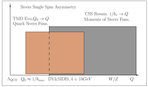
Meanwhile, for moderate $Q^{2}$ variation, there is an alternative approach to apply, from which we can directly solve the evolution by an integral of the kernel from low to high $Q$ Ji:2004wu . This is, in particular, useful at relative low $Q$ region, and can be applied to describe the transverse momentum distributions in SIDIS from HERMES/COMPASS experiments and fixed target Drell-Yan lepton pair production experiments Sun:2013dya . This will also help to build a connection to the ultimate CSS resummation in Drell-Yan and $W/Z$ production. As illustrated in Fig. 1, in the moderate $Q$ region (including HERMES/COMPASS kinematics of SIDIS and Drell-Yan process in fixed target experiments), we apply the evolution by a direct integral of the kernel from relative low $Q$ to relative high $Q$. In the high $Q$ region which covers Drell-Yan lepton pair production and $W/Z$ production, we apply the complete CSS resummation with $b_{*}$-prescription (following BLNY/KN parameterization of the non-perturbative form factors). In the overlap region, we shall obtain a consistent picture for the transverse momentum distribution of the cross section and the spin asymmetries.

Following this procedure, we will determine the quark Sivers functions from the HERMES/COMPASS experiments in SIDIS with $Q^{2}$-evolution taken into account using direct integral of the kernel. In particular, we constrain the transverse momentum moments of the quark Sivers functions, which correspond to the twist-three quark-gluon-quark correlation functions (so-called Qiu-Sterman matrix elements Efremov:1981sh ; Qiu:pp ). These are the bases to evaluate the Sivers single spin asymmetries in the CSS resummation formalism Kang:2011mr . We then calculate the Sivers asymmetries in Drell-Yan processes with the constrained Sivers functions. The consistent check is carried out by comparing the predictions between the evolutions done with direct integral of the kernel from $Q_{0}$ to $Q$ and that with CSS resummation with integral of the kernel from $1/b_{*}$ to $Q$. We notice that in the original BLNY parameterization, there is a strong $x$-dependence (which is correlated to the $Q^{2}$-dependence) in the non-perturbative form factor Landry:2002ix . To avoid this strong dependence, we follow an updated fit by Konychev and Nadolsky Konychev:2005iy which describes equally well the Drell-Yan and W/Z boson data with a mild dependence on $x$. We would like to emphasize that the Sivers asymmetries observed in HERMES/COMPASS experiments mainly focus on the moderate $x$-region around 0.1, which is also the typical $x$-range for the Drell-Yan fixed target experiments .

The rest of the paper is organized as follows. In Sec.II, we present a brief review on the theory of low transverse momentum hard processes as a self-contained introduction. In particular, we will present the detailed derivations of our previous publication of Ref. Kang:2011mr . We will also discuss various TMD factorizations. In Sec.III, we discuss the TMD evolution and resummation in the context of the transverse momentum dependent differential cross sections and the Sivers single spin asymmetries. We will illustrate the incompatibility between the BLNY parameterization of the CSS resummation and the HERMES/COMPASS measurements of the $p_{\perp}$ distribution in SIDIS process. We will also discuss in detail our approach to calculate the transverse momentum distribution in this kinematic region, and compare to the experimental data on multiplicity distribution in SIDIS from HERMES/COMPASS experiments and Drell-Yan fixed target experiments, and demonstrate that our approach consistently describe these data with the TMD evolution taken into account. In Sec.IV, we extend the evolution effects to the Sivers single spin asymmetries measured by the HERMES/COMPASS collaborations, and perform a combined analysis. In Sec. V, we present the predictions for the Sivers asymmetries in Drell-Yan lepton pair productions in the planed experiments, and $W^{\pm}$ production at RHIC. We demonstrate the matching between two different calculations. With this, we show the results for the proposed Drell-Yan experiments. We will emphasize the test of the sign change between SIDIS and Drell-Yan, and highlight the ability to separate the flavor dependence by combining Drell-Yan/W measurements with SIDIS results as well. In Sec. VI, we summarize our paper, and discuss further developments.

II Theory Review of Low Transverse Momentum Hard Processes

In this section, we present a brief review of the theory background for low transverse momentum hard processes. Under the context of this paper, the hard processes are hadronic processes with two separate scales: the invariant mass of virtual photon $Q$ and the transverse momentum of observed particles $q_{\perp}$ for lepton pair in Drell-Yan process or $P_{h\perp}$ for final state hadron in SIDIS.

TMD factorization applies in the kinematic region of low transverse momentum: $q_{\perp}\ll Q$. As mentioned in the Introduction, large double logarithms will arise from perturbative gluon radiation. These large logs have been demonstrated in the single transverse spin dependent differential cross sections as well Ji:2006ub ; Kang:2011mr . In the following, we will summarize these calculations, and, in particular, present detailed derivations of our previous publication Kang:2011mr . We will start with the low transverse momentum Drell-Yan lepton pair productions for both spin averaged and spin-dependent cross sections. We then examine the TMD factorization. Finally, we extend the discussions to the SIDIS process.

II.1 Low Transverse Momentum Drell-Yan

In the Drell-Yan lepton pair production in $pp$ collisions, we have

$$A(P_{A},S_{\perp})+B(P_{B})\to\gamma^{*}(q)+X\to\ell^{+}+\ell^{-}+X,$$ (1)

where $P_{A}$ and $P_{B}$ represent the momenta of hadrons $A$ and $B$, and $S_{\perp}$ for the transverse polarization vector of $A$, respectively. We further assume hadron $A$ moving in the $+\hat{z}$ direction. Light-cone momentum $p^{\pm}$ is defined as $p^{\pm}=1/\sqrt{2}(p^{0}\pm p^{z})$. Therefore, $P_{A}$ is dominated by its plus component, whereas $P_{B}$ by its minus component. The single transverse spin dependent differential cross section can be expressed as

$$\frac{d\Delta\sigma(S_{\perp})}{dydQ^{2}d^{2}q_{\perp}} = \sigma_{0}^{\rm(DY)}\left(W_{UU}(Q;q_{\perp})+\epsilon^{\alpha\beta}S_{\perp}^{\alpha}W_{UT}^{\beta}(Q;q_{\perp})\right)\ ,$$ (2)

where $q_{\perp}$ and $y$ are transverse momentum and rapidity of the lepton pair, $\sigma_{0}^{\rm(DY)}=4\pi\alpha_{em}^{2}/3N_{c}sQ^{2}$ with $s=(P_{A}+P_{B})^{2}$, and $\epsilon^{\alpha\beta}$ is defined as $\epsilon^{\alpha\beta\mu\nu}P_{A\mu}P_{B\nu}/P_{A}\cdot P_{B}$. When $q_{\perp}\ll Q$, the structure function $W_{UT}$ can be formulated in terms of the TMD factorization where the quark Sivers function is involved Brodsky:2002cx ; Collins:2002kn , whereas when $q_{\perp}\gg\Lambda_{\rm QCD}$ it can be calculated in the collinear factorization approach in terms of the twist-three quark-gluon-quark correlation functions Ji:2006ub ; Efremov:1981sh ; Qiu:pp . It has been shown that the TMD and collinear twist-three approaches give the consistent results in the intermediate transverse momentum region: $\Lambda_{\rm QCD}\ll q_{\perp}\ll Q$ Ji:2006ub ; bbdm . This consistency allows us to separate $W_{UT}$ into two terms Collins:1984kg ,

$$W_{UU}(Q;q_{\perp}) = \int\frac{d^{2}b}{(2\pi)^{2}}e^{i\vec{q}_{\perp}\cdot\vec{b}}\widetilde{W}_{UU}(Q;b)+Y_{UU}^{\alpha}(Q;q_{\perp})\ ,$$

$$W_{UT}^{\alpha}(Q;q_{\perp}) = \int\frac{d^{2}b}{(2\pi)^{2}}e^{i\vec{q}_{\perp}\cdot\vec{b}}\widetilde{W}_{UT}^{\alpha}(Q;b)+Y_{UT}^{\alpha}(Q;q_{\perp})\ ,$$

where the first term dominates in the $q_{\perp}\ll Q$ region, while the second term dominates in the region of $q_{\perp}\sim Q$ and $q_{\perp}>Q$. The latter is obtained by subtracting the the leading term of $q_{\perp}^{2}/Q^{2}$ from the full perturbative calculation. In this paper, we focus on the low transverse momentum region, where a TMD factorization is appropriate. We will review how perturbative corrections modify the differential cross sections, in particular, from the large logarithms in fixed order calculations. The results for $\widetilde{W}_{UU,UT}$ up to one-loop corrections will be shown.

II.2 Perturbative Contribution in the Small $b_{\perp}$ Region

To study the QCD dynamics, in particular, to understand the scale evolution of the TMDs, it is illustrative to have a perturbative calculation for the above quantities at small $b_{\perp}$ limit. It is straightforward to write down the leading Born diagram contributions to $\widetilde{W}_{UU}$ and $\widetilde{W}_{UT}$,

$$\widetilde{W}_{UU}^{(0)}(Q,b) = q(z_{1})\bar{q}(z_{2})\ ,$$

$$\widetilde{W}_{UT}^{(0)\alpha}(Q,b) = \left(\frac{-ib_{\perp}^{\alpha}}{2}\right)T_{F}(z_{1},z_{1})\bar{q}(z_{2})\ ,$$ (3)

where $z_{1}=Q/\sqrt{s}e^{y}$, $z_{2}=Q/\sqrt{s}e^{-y}$, $q(z_{1})$ and $\bar{q}(z_{2})$ are the integrated quark and antiquark distribution functions. The single transverse spin asymmetry comes from the quark Sivers function $T_{F}(z_{1},z_{1})=\int d^{2}k_{\perp}k_{\perp}^{2}/Mf_{1T}^{\perp(DY)}(z_{1},k_{\perp})$. The Sivers function $f_{1T}^{\perp}$ follows the Trento convention Bacchetta:2004jz . Since it is process dependent, we adopt that in the Drell-Yan process to calculate the transverse-momentum moment, which is also defined as twist-three quark-gluon-quark correlation function,

$$T_{F}(x_{1},x_{2}) = \int\frac{d\xi^{-}d\eta^{-}}{4\pi}e^{i(k_{q1}^{+}\eta^{-}+k_{g}^{+}\xi^{-})}\,\epsilon_{\perp}^{\beta\alpha}S_{\perp\beta}$$ (4)

$$\times\left\langle PS|\overline{\psi}(0){\cal L}(0,\xi^{-})\gamma^{+}gF_{\alpha}^{\ +}(\xi^{-}){\cal L}(\xi^{-},\eta^{-})\psi(\eta^{-})|PS\right\rangle\ ,$$

where $x_{1}=k_{q1}^{+}/P^{+}$ and $x_{2}=k_{q2}^{+}/P^{+}$ , while $x_{g}=k_{g}^{+}/P^{+}=x_{2}-x_{1}$, ${\cal L}$ is the light-cone gauge link to make the above definition gauge invariant.

At one-loop order, the gluon radiation contribution comes from real and virtual diagrams. The real diagrams have been calculated in the literature Ji:2006ub , and we can write down the results as Ji:2006ub

$$W_{UU}(Q,q_{\perp})|_{q_{\perp}\ll Q} = \frac{\alpha_{s}}{2\pi^{2}}C_{F}\frac{1}{q_{\perp}^{2}}\int\frac{dx}{x}\frac{dx^{\prime}}{x^{\prime}}q(x)\bar{q}(x^{\prime})\left\{\left[\left(\frac{1+\xi_{1}^{2}}{(1-\xi_{1})_{+}}+\frac{D-2}{2}(1-\xi_{2})\right)\delta(1-\xi_{1})\right.\right.$$ (5)

$$\left.\left.+(\xi_{1}\leftrightarrow\xi_{2})\right]+2\delta(1-\xi_{1})\delta(1-\xi_{2})\ln\frac{Q^{2}}{q_{\perp}^{2}}\right\}$$

$$W_{UT}^{\alpha}(Q,q_{\perp})|_{q_{\perp}\ll Q} = \frac{\alpha_{s}}{2\pi^{2}}\frac{q_{\perp}^{\alpha}}{(q_{\perp}^{2})^{2}}\int\frac{dx}{x}\frac{dx^{\prime}}{x^{\prime}}\bar{q}(x^{\prime})\left\{T_{F}(x,x)\delta(1-\xi_{1})\left(\frac{1+\xi_{2}^{2}}{(1-\xi_{2})_{+}}+\frac{D-2}{2}(1-\xi_{2})\right)\right.$$ (6)

$$\left.+2C_{F}T_{F}(x,x)\delta(1-\xi_{1})\delta(1-\xi_{2})\ln\frac{Q^{2}}{q_{\perp}^{2}}+\delta(1-\xi_{2})\frac{C_{A}}{2}T_{F}(x,z_{1})\frac{1+\xi_{1}}{(1-\xi_{1})_{+}}\right.$$

$$\left.+\delta(1-\xi_{2})\frac{1}{2N_{C}}\left[\left(x\frac{\partial}{\partial x}T_{F}(x,x)\right)(1+\xi_{1}^{2})+T_{F}(x,x)\frac{(1-\xi_{1})^{2}(2\xi_{1}+1)-2}{(1-\xi_{1})_{+}}\right]\right.$$

$$\left.+\delta(1-\xi_{2})\frac{1}{2N_{C}}T_{F}(x,x)\frac{D-2}{2}(1-\xi_{1})\right\}\ ,$$

where $\xi_{1}=z_{1}/x$ and $\xi_{2}=z_{2}/x^{\prime}$, and we have kept the $\epsilon=(2-D)/2$ (with $D$ represents the transverse dimension in the dimension regulation) term in the above calculations. After Fourier transformation into the impact parameter space, this will lead to a finite contribution. In the above results, we only keep the soft and hard gluon pole contributions in the $q\bar{q}$ channel for the single spin asymmetry calculations. All other contributions can be formulated similarly.

Applying the Fourier transform formulas we listed in the Appendix, we obtain the following result for the real gluon radiation contribution to $\widetilde{W}_{UU}(Q;b)$ at one-loop order,

$$\widetilde{W}_{UU}^{(r)}(b) = \frac{\alpha_{s}}{2\pi}C_{F}\left\{\left[-\frac{1}{\epsilon}+\ln\frac{c_{0}^{2}}{b_{\perp}^{2}\mu^{2}}\right]\left[\frac{1+\xi_{1}^{2}}{(1-\xi_{1})_{+}}\delta(1-\xi_{2})+\frac{1+\xi_{2}^{2}}{(1-\xi_{2})_{+}}\delta(1-\xi_{1})\right]\right.$$ (7)

$$+2\delta(1-\xi_{1})\delta(1-\xi_{2})\left[\frac{1}{\epsilon^{2}}-\frac{1}{\epsilon}\ln\frac{Q^{2}}{\mu^{2}}+\frac{1}{2}\left(\ln\frac{Q^{2}}{\mu^{2}}\right)^{2}-\frac{1}{2}\left(\ln\frac{Q^{2}b_{\perp}^{2}}{c_{0}^{2}}\right)^{2}-\frac{\pi^{2}}{12}\right]$$

$$\left.+(1-\xi_{1})\delta(1-\xi_{2})+(1-\xi_{2})\delta(1-\xi_{1})\right\}\ ,$$

where $c_{0}=2e^{-\gamma_{E}}$ and a common integral $\int dxdx^{\prime}/xx^{\prime}$ as that in Eq. (6) has been omitted for simplicity. To arrive the above result, we have applied the $\overline{\rm MS}$ subtraction scheme with $\mu^{2}\rightarrow 4\pi e^{-\gamma_{E}}\mu^{2}$. This is different from the $\overline{\rm MS}$ used in the Collins book Collins (see the discussions below).

The above result contains collinear and soft divergences. The soft divergences shall be cancelled by the virtual diagrams, whereas the collinear divergences absorbed into the renormalization of the parton distributions. The virtual diagrams contributes

$$\widetilde{W}_{UU}^{(v)}=\frac{\alpha_{s}}{2\pi}\left[-\frac{2}{\epsilon^{2}}-\frac{3}{\epsilon}+\frac{2}{\epsilon}\ln\frac{Q^{2}}{\mu^{2}}+\frac{7}{6}\pi^{2}+3\ln\frac{Q^{2}}{\mu^{2}}-\left(\ln\frac{Q^{2}}{\mu^{2}}\right)^{2}-8\right]\delta(1-\xi_{1})\delta(1-\xi_{2})\ .$$ (8)

Adding them together, we will have

$$\widetilde{W}_{UU}(Q,b) = \frac{\alpha_{s}}{2\pi}C_{F}\left\{\left(-\frac{1}{\epsilon}+\ln\frac{c_{0}^{2}}{b^{2}\mu^{2}}\right)\left({\cal P}_{q\to q}(\xi_{1})\delta(1-\xi_{2})+{\cal P}_{q\to q}(\xi_{2})\delta(1-\xi_{1})\right)\right.$$ (9)

$$+(1-\xi_{1})\delta(1-\xi_{2})+(1-\xi_{2})\delta(1-\xi_{1})$$

$$\left.+\delta(1-\xi_{1})\delta(1-\xi_{2})\left[3\ln\frac{Q^{2}b^{2}}{c_{0}^{2}}-\left(\ln\frac{Q^{2}b^{2}}{c_{0}^{2}}\right)^{2}+\pi^{2}-8\right]\right\}\ ,$$

where ${\cal P}_{q\to q}(\xi)=\left(\frac{1+\xi^{2}}{1-\xi}\right)_{+}$ is the quark splitting kernel.

Similarly, for the single-spin dependent cross section, we have for the real diagram contributions,

$$\widetilde{W}_{UT}^{\alpha(r)} = \frac{\alpha_{s}}{2\pi}\left(\frac{-ib_{\perp}^{\alpha}}{2}\right)\bar{q}(x^{\prime})\left\{\left(-\frac{1}{\epsilon}+\ln\frac{c_{0}^{2}}{b_{\perp}^{2}\mu^{2}}\right)\left[\frac{1+\xi_{2}^{2}}{(1-\xi_{2})_{+}}T_{F}(x,x)\delta(1-\xi_{1})+\delta(1-\xi_{2})\right.\right.$$ (10)

$$\left.\times\left(\frac{C_{A}}{2}T_{F}(x,z_{1})\frac{1+\xi_{1}}{(1-\xi_{1})_{+}}+\frac{1}{2N_{C}}T_{F}(x,x)\left(\frac{-1-\xi_{1}^{2}}{(1-\xi_{1})_{+}}-2\delta(1-\xi_{1})\right)\right)\right]$$

$$+2C_{F}T_{F}(x,x)\delta(1-\xi_{1})\delta(1-\xi_{2})\left[\frac{1}{\epsilon^{2}}-\frac{1}{\epsilon}\ln\frac{Q^{2}}{\mu^{2}}+\frac{1}{2}\left(\ln\frac{Q^{2}}{\mu^{2}}\right)^{2}-\frac{1}{2}\left(\ln\frac{Q^{2}b_{\perp}^{2}}{c_{0}^{2}}\right)^{2}-\frac{\pi^{2}}{12}\right]$$

$$-2C_{F}T_{F}(x,x)\delta(1-\xi_{1})\delta(1-\xi_{2})\left(-\frac{1}{\epsilon}+\ln\frac{c_{0}^{2}}{b^{2}\mu^{2}}\right)$$

$$\left.+\left(-\frac{1}{2N_{c}}\right)T_{F}(x,x)(1-\xi_{1})\delta(1-\xi_{2})+C_{F}T_{F}(x,x)(1-\xi_{2})\delta(1-\xi_{1})\right\}\ ,$$

where we have simplified the expression by integrating out the partial derivative in Eq. (6). The last second line comes from the second term in the Fourier transform formula of Eq. (98) in the Appendix . The virtual contribution has the similar form as Eq. (8). After adding them together, we find that the total contribution at one-loop order,

$$W_{UT} = \frac{\alpha_{s}}{2\pi}\left(\frac{-ib_{\perp}^{\alpha}}{2}\right)\left\{\left(-\frac{1}{\epsilon}+\ln\frac{c_{0}^{2}}{b^{2}\mu^{2}}\right)\left({\cal P}_{qg\to qg}^{T}\otimes T_{F}(z_{1})\delta(1-\xi_{2})+C_{F}{\cal P}_{q\to q}(\xi_{2})T_{F}(z_{1},z_{1})\delta(1-\xi_{1})\right)\right.$$ (11)

$$+T_{F}(x,x)\left[\left(-\frac{1}{2N_{c}}\right)(1-\xi_{1})\delta(1-\xi_{2})+C_{F}(1-\xi_{2})\delta(1-\xi_{1})\right]$$

$$\left.+\delta(1-\xi_{1})\delta(1-\xi_{2})T_{F}(z_{1},z_{1})C_{F}\left[3\ln\frac{Q^{2}b^{2}}{c_{0}^{2}}-\left(\ln\frac{Q^{2}b^{2}}{c_{0}^{2}}\right)^{2}+\pi^{2}-8\right]\right\}\ ,$$

where ${\cal P}_{q\to q}(\xi)$ is the same as above, and the splitting kernel for the Sivers function can be written as

$${\cal P}_{qg\to qg}^{T}\otimes T_{F}(z) = \int\frac{dx}{x}\left\{T_{F}(x,x)\left[C_{F}\left(\frac{1+\xi^{2}}{1-\xi}\right)_{+}-C_{A}\delta(1-\xi)\right]\right.$$ (12)

$$\left.+\frac{C_{A}}{2}\left(T_{F}(x,z)\frac{1+\xi}{1-\xi}-T_{F}(x,x)\frac{1+\xi^{2}}{1-\xi}\right)\right\}\ ,$$

which agrees with recent calculations for the splitting kernel for the part involved in the above calculations Braun:2009mi ; Schafer:2012ra ; Kang:2012em ; Ma:2012xn .

In the above results, the one-loop corrections Eqs. (9,11) clearly demonstrate large logarithms. To resum these large logs, we need to apply the TMD factorization, and solve the relevant evolution equation. Although the different TMD schemes have been used in the literature, the final evolution for the structure functions $\widetilde{W}_{UU,UT}$ remain the same. First, we examine the TMD factorization for the perturbative calculations at one-loop order.

II.3 Sivers Quark Distributions and TMD factorization

To demonstrate the factorization, we calculate the TMD quark and antiquark distributions, and show that the collinear part of the structure functions calculated in the last subsection can be absorbed into these TMD distributions. It has been known that, however, there is scheme-dependence in the TMD definitions. Therefore, the hard factors will also depend on which scheme you choose to calculate the TMDs. The scheme dependence comes from the fact that the TMD distributions have light-cone singularity, and different ways to regulate this singularity define different schemes of the TMD distributions.

II.3.1 Ji-Ma-Yuan Scheme

In the Ji-Ma-Yuan scheme, the light-cone gauge link in the TMD definition is chosen to be slightly off-light-cone, $n=(1^{-},0^{+},0_{\perp})\to v=(v^{-},v^{+},0_{\perp})$ with $v^{-}\gg v^{+}$. Similarly, for the TMD for the antiquark distribution, $\tilde{v}$ was introduced, $\tilde{v}=(\tilde{v}^{-},\tilde{v}^{+},0_{\perp})$ with $\tilde{v}^{+}\gg\tilde{v}^{-}$. Because of the additional $v$ and $\tilde{v}$, there are additional invariants: $\zeta_{1}^{2}=(2v\cdot P_{A})^{2}/v^{2}$, $\zeta_{2}^{2}=(2\tilde{v}\cdot P_{B})^{2}/\tilde{v}^{2}$, and $\rho^{2}=(2v\cdot\tilde{v})^{2}/v^{2}\tilde{v}^{2}$. The TMD quark distributions of a polarized proton is defined through the following matrix:

$${\cal M}^{\alpha\beta} = P^{+}\int\frac{d\xi^{-}}{2\pi}e^{-ix\xi^{-}P^{+}}\int\frac{d^{2}b_{\perp}}{(2\pi)^{2}}e^{i\vec{b}_{\perp}\cdot\vec{k}_{\perp}}$$ (13)

$$\times\left\langle PS\left|\overline{\psi}^{\beta}(\xi^{-},0,\vec{b}_{\perp}){\cal L}_{v}^{\dagger}(-\infty;\xi){\cal L}_{v}(-\infty;0)\psi^{\alpha}(0)\right|PS\right\rangle\ ,$$

with the gauge link

$${\cal L}_{v}(-\infty;\xi)\equiv\exp\left(-ig\int^{-\infty}_{0}d\lambda\,v\cdot A(\lambda v+\xi)\right)\ .$$ (14)

This gauge link goes to $-\infty$, indicating that we adopt the definition for the TMD quark distributions for the Drell-Yan process. Keeping only the unpolarized quark distribution and the Sivers function, we have the following expansion for the matrix ${\cal M}$:

$${\cal M}=\frac{1}{2}\left[q(x,k_{\perp})\gamma_{\mu}P^{\mu}+\frac{1}{M}\,f_{1T}^{\perp}(x,k_{\perp})\,\epsilon_{\mu\nu\alpha\beta}\gamma^{\mu}P^{\nu}k^{\alpha}S^{\beta}+\ldots\right]$$ (15)

where $q(x,k_{\perp})$ is the TMD distribution in an unpolarized proton, $f_{1T}^{\perp}(x,k_{\perp})$ is the Sivers function, and $M$ is a hadron mass, used to normalize $q(x,k_{\perp})$ and $f_{1T}^{\perp}(x,k_{\perp})$ to the same mass dimension.

First, the soft factor has been calculated,

$$S(b_{\perp})=\frac{\alpha_{s}}{2\pi}C_{F}\ln\frac{b^{2}\mu^{2}}{c_{0}^{2}}\left(2-\ln\rho^{2}\right)\ .$$ (16)

The calculations of the TMDs in the Ji-Ma-Yuan is straightforward, and we find that the quark distribution can be written as,

$$q(z,k_{\perp})|_{real}=\frac{\alpha_{s}}{2\pi^{2}}\frac{1}{k_{\perp}^{2}}C_{F}\int\frac{dx}{x}q(x)\left\{\frac{1+\xi^{2}}{(1-\xi)_{+}}+\frac{D-2}{2}(1-\xi)+\delta(1-\xi)\left(\ln\frac{z^{2}\zeta^{2}}{k_{\perp}^{2}}-1\right)\right\}\ ,$$ (17)

where $\xi=z/x$ and in the impact parameter space,

$$q(z,b_{\perp})|_{real} = \frac{\alpha_{s}}{2\pi}C_{F}\left\{\left(-\frac{1}{\epsilon}+\ln\frac{c_{0}^{2}}{b^{2}\mu^{2}}\right)\left[\frac{1+\xi^{2}}{(1-\xi_{1})_{+}}-\delta(1-\xi)\right]+(1-\xi)\right.$$ (18)

$$\left.+\delta(1-\xi)\left[\frac{1}{\epsilon^{2}}-\frac{1}{\epsilon}\ln\frac{z^{2}\zeta^{2}}{\mu^{2}}+\frac{1}{2}\left(\ln\frac{z^{2}\zeta^{2}}{\mu^{2}}\right)^{2}-\frac{1}{2}\left(\ln\frac{z^{2}\zeta^{2}b_{\perp}^{2}}{c_{0}^{2}}\right)^{2}-\frac{\pi^{2}}{12}\right]\right\}\ .$$

The virtual diagram contributes,

$$q(z,b_{\perp})|_{vir} = \frac{\alpha_{s}}{2\pi}\delta(1-\xi)\left[-\frac{1}{\epsilon^{2}}-\frac{5}{2\epsilon}+\frac{1}{\epsilon}\ln\frac{\zeta^{2}}{\mu^{2}}+\ln\frac{\zeta^{2}}{\mu^{2}}-\frac{1}{2}\left(\ln\frac{z^{2}\zeta^{2}}{\mu^{2}}\right)^{2}-\frac{5}{12}\pi^{2}-2\right]\ .$$ (19)

Adding them together, we have

$$q(z,b_{\perp}) = \frac{\alpha_{s}}{2\pi}C_{F}\left\{\left(-\frac{1}{\epsilon}+\ln\frac{c_{0}^{2}}{b^{2}\bar{\mu}^{2}}\right){\cal P}_{q\to q}(\xi)-\delta(1-\xi)\ln\frac{c_{0}^{2}}{b^{2}\mu^{2}}+(1-\xi)\right.$$ (20)

$$\left.+\delta(1-\xi)\left[\frac{3}{2}\ln\frac{b^{2}\mu^{2}}{c_{0}^{2}}+\ln\frac{z^{2}\zeta^{2}}{\mu^{2}}-\frac{1}{2}\left(\ln\frac{z^{2}\zeta^{2}b_{\perp}^{2}}{c_{0}^{2}}\right)^{2}-2-\frac{\pi^{2}}{2}\right]\right\}\ .$$

Similar expression can be written for the antiquark distribution. According to the TMD factorization, we can subtract the quark distribution, antiquark distribution and the soft factor, and obtain the hard factor,

$$W_{UU}(Q;b)=q(z_{1},b,\zeta_{1})\bar{q}(z_{2},b,\zeta_{2})H_{UU}(Q)\left(S(b,\rho)\right)^{-1}\ .$$ (21)

Applying these results, we have the following result for the hard factor,

$$H_{UU}(Q)=\frac{\alpha_{s}}{2\pi}C_{F}\left[\ln\frac{Q^{2}}{\mu^{2}}+\ln\rho^{2}\ln\frac{Q^{2}}{\mu^{2}}-\ln\rho^{2}+\ln^{2}\rho+2\pi^{2}-4\right]\ ,$$ (22)

where $z_{1}^{2}z_{2}^{2}\zeta_{1}^{2}\zeta_{2}^{2}=\rho^{2}Q^{4}$ has been used to simplify the hard factor.

We can follow the same procedure to calculate that for the Sivers asymmetry. The TMD quark Sivers function can be written as,

$$f_{1T}^{\perp}(z,k_{\perp}) = \frac{\alpha_{s}}{2\pi^{2}}\frac{M}{(k_{\perp}^{2})^{2}}\int\frac{dx}{x}\left\{\frac{C_{A}}{2}T_{F}(x,z)\frac{1+\xi}{(1-\xi)_{+}}+T_{F}(x,x)\frac{-1}{2N_{c}}\frac{D-2}{2}(1-\xi)\right.$$ (23)

$$+\frac{1}{2N_{C}}\left[\left(x\frac{\partial}{\partial x}T_{F}(x,x)\right)(1+\xi^{2})+T_{F}(x,x)\frac{(1-\xi)^{2}(2\xi+1)-2}{(1-\xi)_{+}}\right]$$

$$\left.+T_{F}(x,x)\delta(1-\xi)C_{F}\left(\ln\frac{x^{2}\zeta^{2}}{k_{\perp}^{2}}-2\right)\right\}\ .$$

We note a factor of (-2) in the last term, which is different from that in Ref. Ji:2006ub . This comes from a sub-leading expansion contribution from the soft-pole and hard-pole diagrams, which was omitted in Ref. Ji:2006ub . This term will contribute to the collinear singularity when Fourier transforming into the impact parameter space. Adding the virtual diagram contributions, we will have total result in the impact parameter space,

$$\tilde{f}_{1T}^{\alpha}(z,b) = \frac{\alpha_{s}}{2\pi}\left(\frac{-ib_{\perp}^{\alpha}}{2}\right)\left\{\left(-\frac{1}{\epsilon}+\ln\frac{c_{0}^{2}}{b^{2}\mu^{2}}\right){\cal P}_{qg\to qg}^{T}\otimes T_{F}(z)\right.$$ (24)

$$-\delta(1-\xi)T_{F}(x,x)C_{F}\ln\frac{c_{0}^{2}}{b^{2}\mu^{2}}-\frac{1}{2N_{c}}T_{F}(x,x)(1-\xi)$$

$$\left.+\delta(1-\xi)T_{F}(x,x)C_{F}\left[\frac{3}{2}\ln\frac{b^{2}\mu^{2}}{c_{0}^{2}}+\ln\frac{z^{2}\zeta^{2}}{\mu^{2}}-\frac{1}{2}\left(\ln\frac{z^{2}\zeta^{2}b_{\perp}^{2}}{c_{0}^{2}}\right)^{2}-2-\frac{\pi^{2}}{2}\right]\right\}\ ,$$

at one-loop order. By subtraction, we obtain the hard factor for the Sivers single spin asymmetry in Drell-Yan process,

$$H_{UT}(Q)=H_{UU}(Q)=\frac{\alpha_{s}}{2\pi}C_{F}\left[\ln\frac{Q^{2}}{\mu^{2}}+\ln\rho^{2}\ln\frac{Q^{2}}{\mu^{2}}-\ln\rho^{2}+\ln^{2}\rho+2\pi^{2}-4\right]\ .$$ (25)

This is an important result, as it shows that the hard factor is spin-independent.

II.3.2 Collins-11

In 2011, Collins introduces a new definition for the TMDs, where the soft gluon and light-cone singularities are subtracted in the TMDs from the beginning. As a result, there is no soft factor in the factorization formula, which is absorbed into the definition of PDF.

From its definition, we find that the real diagram contribution can be written as Collins

$$q_{\rm JCC}(z,k_{\perp})|_{real}=\frac{\alpha_{s}}{2\pi^{2}}\frac{1}{k_{\perp}^{2}}C_{F}\int\frac{dx}{x}q(x)\left\{\frac{1+\xi^{2}}{(1-\xi)_{+}}+\frac{D-2}{2}(1-\xi)+\delta(1-\xi)\left(\ln\frac{\zeta_{c}^{2}}{k_{\perp}^{2}}\right)\right\}\ ,$$ (26)

where $\zeta_{c}$ is defined as $\zeta_{c}^{2}=(z_{1}P_{A}^{+})^{2}e^{-2y_{n}}$ with $y_{n}$ the rapidity cutoff to regulate the light-cone singularity. The virtual diagram for $q_{\rm JCC}$ only contributes to the counter terms,

$$q_{\rm JCC}(z,b_{\perp})|_{vir} = \frac{\alpha_{s}}{2\pi}\delta(1-\xi)\left[-\frac{1}{\epsilon^{2}}-\frac{3}{2\epsilon}+\frac{1}{\epsilon}\ln\frac{\zeta_{c}^{2}}{\mu^{2}}\right]\ ,$$ (27)

where, to be consistent, we have followed the $S_{\epsilon}=(4\pi)^{\epsilon}/\Gamma(1-\epsilon)$ prescription of $\overline{\rm MS}$ subtraction of Ref. Collins .

Therefore, the total quark distribution can be written as,

$$q_{\rm JCC}(z,b_{\perp}) = \frac{\alpha_{s}}{2\pi}C_{F}\left\{\left(-\frac{1}{\epsilon}+\ln\frac{c_{0}^{2}}{b^{2}\bar{\mu}^{2}}\right){\cal P}_{q\to q}(\xi)+(1-\xi)\right.$$ (28)

$$\left.+\delta(1-\xi)\left[\frac{3}{2}\ln\frac{b^{2}\mu^{2}}{c_{0}^{2}}+\frac{1}{2}\left(\ln\frac{\zeta_{c}^{2}}{\mu^{2}}\right)^{2}-\frac{1}{2}\left(\ln\frac{\zeta_{c}^{2}b_{\perp}^{2}}{c_{0}^{2}}\right)^{2}\right]\right\}\ .$$

We notice that an additional term of $(-\frac{\pi^{2}}{12})$ shall be added to the above equation if we use the $\overline{\rm MS}$ subtraction method of the last subsection, see, also the detailed discussions in Ref. Collins:2012uy . To calculate the hard factor in this scheme, we apply the factorization

$$W_{UU}(Q;b)=q_{\rm JCC}(z_{1},b,\zeta_{c})\bar{q}_{\rm JCC}(z_{2},b,\zeta_{\bar{c}})H_{UU}^{(\rm JCC)}(Q)\ .$$ (29)

The hard factor can be calculated Collins ,

$$H_{UU}^{(\rm JCC)}(Q)=\frac{\alpha_{s}}{2\pi}C_{F}\left[3\ln\frac{Q^{2}}{\mu^{2}}+\ln^{2}\frac{Q^{2}}{\mu^{2}}+\frac{1}{2}\pi^{2}-8\right]\ ,$$ (30)

We notice that the different $\overline{\rm MS}$ subtraction method will lead to different hard factors in Collins-11 scheme for the TMD definition Collins:2012uy . In particular, the $\overline{\rm MS}$ subtraction used in the last sub-section will add additional term of $\pi^{2}/6$ in the above hard factor. This is because the Collins-11 definition of the TMD distribution, there is a double pole $1/\epsilon^{2}$ in the UV divergence in the dimensional regulation for the virtual diagram Collins:2012uy .

For the Sivers function, the calculations can follow similarly. The real diagram contribution for the quark Sivers function can be calculated in the Collins-11 definition,

$$f_{1T}^{({\rm JCC})\perp}(z,k_{\perp}) = \frac{\alpha_{s}}{2\pi^{2}}\frac{M}{(k_{\perp}^{2})^{2}}\int\frac{dx}{x}\left\{\frac{C_{A}}{2}T_{F}(x,z)\frac{1+\xi}{(1-\xi)_{+}}+T_{F}(x,x)\frac{-1}{2N_{c}}\frac{D-2}{2}(1-\xi)\right.$$ (31)

$$+\frac{1}{2N_{C}}\left[\left(x\frac{\partial}{\partial x}T_{F}(x,x)\right)(1+\xi^{2})+T_{F}(x,x)\frac{(1-\xi)^{2}(2\xi+1)-2}{(1-\xi)_{+}}\right]$$

$$\left.+T_{F}(x,x)\delta(1-\xi)C_{F}\left(\ln\frac{\zeta_{c}^{2}}{k_{\perp}^{2}}-1\right)\right\}\ .$$

Virtual diagram is the same as the unpolarized case, and the total quark Sivers function in $b$-space,

$$\tilde{f}_{1T}^{({\rm JCC})\alpha}(z,b) = \frac{\alpha_{s}}{2\pi}\left(\frac{-b_{\perp}^{\alpha}}{2}\right)\left\{\left(-\frac{1}{\epsilon}+\ln\frac{c_{0}^{2}}{b^{2}\mu^{2}}\right){\cal P}_{qg\to qg}^{T}\otimes T_{F}(z)-\frac{1}{2N_{c}}T_{F}(x,x)(1-\xi)\right.$$ (32)

$$\left.+\delta(1-\xi)C_{F}\left[\frac{3}{2}\ln\frac{b^{2}\mu^{2}}{c_{0}^{2}}+\frac{1}{2}\left(\ln\frac{\zeta_{c}^{2}}{\mu^{2}}\right)^{2}-\frac{1}{2}\left(\ln\frac{\zeta_{c}^{2}b_{\perp}^{2}}{c_{0}^{2}}\right)^{2}\right]\right\}\ ,$$

where, again, we have followed the $S_{\epsilon}$ prescription for $\overline{\rm MS}$ subtraction in Collins-11 definition of the TMDs. Again, we find that the hard factor can be calculated

$$H_{UT}^{(c)}(Q)=H_{UU}^{(c)}(Q)=\frac{\alpha_{s}}{2\pi}C_{F}\left[3\ln\frac{Q^{2}}{\mu^{2}}+\ln^{2}\frac{Q^{2}}{\mu^{2}}+\frac{1}{2}\pi^{2}-8\right]\ .$$ (33)

Again, if we choose the $\overline{\rm MS}$ subtraction method of the last sub-section, we would add additional term of $\pi^{2}/6$ to the above hard factor.

II.3.3 Echevarria-Idilbi-Scimemi (EIS)

In a recent publication by Collins and Rogers Collins:2012uy , it has been shown that EIS version GarciaEchevarria:2011rb of the soft-collinear-effective-theory approach for the TMD quark distribution is equivalent to that of the Collins-11 approach. Therefore, the calculations in the previous subsection can be carried out similarly for EIS TMD quark distributions. We omit the details of this calculation.

II.4 Semi-inclusive DIS

In this subsection, we briefly review the calculations for the semi-inclusive hadron production in deep inelastic scattering. Much of the results presented above can be followed. For SIDIS, we have,

$$e(\ell)+p(P)\to e(\ell^{\prime})+h(P_{h})+X\ ,$$ (34)

which proceeds through exchange of a virtual photon with momentum $q_{\mu}=\ell_{\mu}-\ell^{\prime}_{\mu}$ and invariant mass $Q^{2}=-q^{2}$. When $P_{h\perp}\ll Q$, the TMD factorization applies, according which the differential SIDIS cross section may be written as

$$\frac{d\sigma(S_{\perp})}{dx_{B}dydz_{h}d^{2}\vec{P}_{h\perp}} = \sigma_{0}^{\rm(DIS)}\times\left[F_{UU}+\epsilon^{\alpha\beta}S_{\perp}^{\alpha}F_{\rm sivers}^{\beta}\right]\ ,$$ (35)

where $\sigma_{0}^{\rm(DIS)}=4\pi\alpha^{2}_{\rm em}S_{ep}/{Q^{4}}\times(1-y+y^{2}/2)x_{B}$ with usual DIS kinematic variables $y$, $x_{B}$ and $Q^{2}$, $z_{h}=P_{h}\cdot P/q\cdot P$, $P_{h\perp}$ the transverse momentum of the final state hadron respect to the lepton plane, and where $\phi_{S}$ and $\phi_{h}$ are the azimuthal angles of the proton’s transverse polarization vector and the transverse momentum vector of the final-state hadron, respectively. We only keep the terms we are interested in: $F_{UU}$ corresponds to the unpolarized cross section, and $F_{\rm sivers}$ to the Sivers function contribution to the single-transverse-spin asymmetry. $F_{UU}$ and $F_{\rm sivers}$ depend on the kinematical variables, $x_{B}$, $z_{h}$, $Q^{2}$, $y$, and $P_{h\perp}$. Similar to that in the Drell-Yan process, at low transverse momentum ($P_{h\perp}\ll Q$) the structure functions can be formulated in terms of the TMD factorization, and they can be written into two terms,

$$F_{UU}(Q;q_{\perp}) = \int\frac{d^{2}b}{(2\pi)^{2}}e^{i\vec{q}_{\perp}\cdot\vec{b}}\widetilde{F}_{UU}(Q;b)+Y_{UU}(Q;q_{\perp})\ ,$$ (36)

$$F_{UT}^{\alpha}(Q;q_{\perp}) = \int\frac{d^{2}b}{(2\pi)^{2}}e^{i\vec{q}_{\perp}\cdot\vec{b}}\widetilde{F}_{UT}^{\alpha}(Q;b)+Y_{UT}^{\alpha}(Q;q_{\perp})\ ,$$ (37)

where the first term dominates in $P_{h\perp}\ll Q$ region, and the second term dominates in the region of $P_{h\perp}\sim Q$ and $P_{h\perp}>Q$. Again, the latter is obtained by subtracting the leading term of $P_{h\perp}^{2}/Q^{2}$ from the full perturbative calculation.

One perturbative gluon radiation contributes to finite $k_{\perp}$ for the differential cross section,

$$F_{UU}|_{P_{h\perp}\ll Q} = \frac{\alpha_{s}}{2\pi^{2}}\frac{1}{\vec{P}_{h\perp}^{2}}C_{F}\int\frac{dxdz}{xz}q(x)D(z)\left\{\left(\frac{1+\xi^{2}}{(1-\xi)_{+}}+\frac{D-2}{2}(1-\xi)\right)\delta(\hat{\xi}-1)\right.$$ (38)

$$\left.+\left(\frac{1+\hat{\xi}^{2}}{(1-\hat{\xi})_{+}}+\frac{D-2}{2}(1-\hat{\xi})\right)\delta(\xi-1)+2\delta(\xi-1)\delta(\hat{\xi}-1)\ln\frac{z_{h}^{2}Q^{2}}{\vec{P}_{h\perp}^{2}}\right\}\ ,$$

where $\xi=x_{B}/x$ and $\hat{\xi}=z_{h}/z$, $q(x)$ represents the integrated quark distribution, $D(z)$ the fragmentation function. Similarly, for the single-transverse-spin dependent cross section, we have

$$F_{UT}^{\beta}|_{P_{h\perp}\ll Q} = -\frac{z_{h}P_{h\perp}^{\beta}}{(\vec{P}_{h\perp}^{2})^{2}}\frac{\alpha_{s}}{2\pi^{2}}\int\frac{dxdz}{xz}D(z)\left\{C_{F}T_{F}(x,x)\delta(\xi-1)\left(\frac{1+\hat{\xi}^{2}}{(1-\hat{\xi})_{+}}+\frac{D-2}{2}(1-\hat{\xi})\right)\right.$$ (39)

$$+\delta(\hat{\xi}-1)\frac{1}{2N_{C}}\left[\left(x\frac{\partial}{\partial x}T_{F}(x,x)\right)(1+\xi^{2})+T_{F}(x,x)\frac{(1-\xi)^{2}(2\xi+1)-2}{(1-\xi)_{+}}\right]$$

$$+\delta(\hat{\xi}-1)\left[\frac{C_{A}}{2}T_{F}(x,x-\widehat{x}_{g})\frac{1+\xi}{(1-\xi)_{+}}+\left(-\frac{1}{2N_{c}}\right)T_{F}(x,x)\frac{D-2}{2}(1-\xi)\right]$$

$$\left.+2\delta(\hat{\xi}-1)\delta(\xi-1)C_{F}T_{F}(x,x)\ln\frac{z_{h}^{2}Q^{2}}{\vec{P}_{h\perp}^{2}}\right\}\ ,$$

where $\hat{x}_{g}=(1-\xi)x=x-x_{B}$.

By applying the Fourier transform (some of the useful integrals are listed in the Appendix), we obtain the following result for $\widetilde{F}_{UU}(Q,b)$ and $\widetilde{F}_{UT}^{\beta}(Q,b)$,

$$\widetilde{F}_{UU}|_{real} = \frac{\alpha_{s}}{2\pi}C_{F}\frac{1}{\hat{\xi}}\left\{\left[-\frac{1}{\epsilon}+\ln\frac{c_{0}^{2}}{b_{\perp}^{2}\mu^{2}}\right]\left[\frac{1+\xi^{2}}{(1-\xi)_{+}}\delta(1-\hat{\xi})+\frac{1+\hat{\xi}^{2}}{(1-\hat{\xi})_{+}}\delta(1-\xi)\right]\right.$$

$$+2\delta(1-\xi)\delta(1-\hat{\xi})\left[\frac{1}{\epsilon^{2}}-\frac{1}{\epsilon}\ln\frac{Q^{2}}{\mu^{2}}+\frac{1}{2}\left(\ln\frac{Q^{2}}{\mu^{2}}\right)^{2}-\frac{1}{2}\left(\ln\frac{Q^{2}b_{\perp}^{2}}{c_{0}^{2}}\right)^{2}-\frac{\pi^{2}}{12}\right]$$

$$\left.+(1-\xi)\delta(1-\hat{\xi})+(1-\hat{\xi})\delta(1-\xi)\right\}\ ,$$

$$\widetilde{F}_{UT}^{\beta}|_{real} = \frac{\alpha_{s}}{2\pi}\frac{1}{\hat{\xi}}\left(\frac{ib_{\perp}^{\alpha}}{2}\right)D(z)\left\{\left(-\frac{1}{\epsilon}+\ln\frac{c_{0}^{2}}{b_{\perp}^{2}\mu^{2}}\right)\left[\frac{1+\hat{\xi}^{2}}{(1-\hat{\xi})_{+}}T_{F}(x,x)\delta(1-\xi)+\delta(1-\hat{\xi})\right.\right.$$ (40)

$$\left.\times\left(\frac{C_{A}}{2}T_{F}(x,z_{1})\frac{1+\xi}{(1-\xi)_{+}}+\frac{1}{2N_{C}}T_{F}(x,x)\left(\frac{-1-\xi^{2}}{(1-\xi)_{+}}-2\delta(1-\xi)\right)\right)\right]$$

$$+2C_{F}T_{F}(x,x)\delta(1-\xi)\delta(1-\hat{\xi})\left[\frac{1}{\epsilon^{2}}-\frac{1}{\epsilon}\ln\frac{Q^{2}}{\mu^{2}}+\frac{1}{2}\left(\ln\frac{Q^{2}}{\mu^{2}}\right)^{2}-\frac{1}{2}\left(\ln\frac{Q^{2}b_{\perp}^{2}}{c_{0}^{2}}\right)^{2}-\frac{\pi^{2}}{12}\right]$$

$$-2C_{F}T_{F}(x,x)\delta(1-\xi)\delta(1-\hat{\xi})\left(-\frac{1}{\epsilon}+\ln\frac{c_{0}^{2}}{b^{2}\mu^{2}}\right)$$

$$\left.+\left(-\frac{1}{2N_{c}}\right)T_{F}(x,x)(1-\xi)\delta(1-\hat{\xi})+C_{F}T_{F}(x,x)(1-\hat{\xi})\delta(1-\xi)\right\}\ ,$$

Clearly, the real diagrams contributions contain soft divergence, which will be cancelled by the virtual diagrams contributions. The virtual diagram contributes to a factor,

$$\frac{\alpha_{s}}{2\pi}\left[-\frac{2}{\epsilon^{2}}-\frac{3}{\epsilon}+\frac{2}{\epsilon}\ln\frac{Q^{2}}{\mu^{2}}+\frac{1}{6}\pi^{2}+3\ln\frac{Q^{2}}{\mu^{2}}-\left(\ln\frac{Q^{2}}{\mu^{2}}\right)^{2}-8\right]\ ,$$ (41)

which differs from that for Drell-Yan process by a term of $\pi^{2}$. After canceling out these divergences, we have the total contribution at one-loop order,

$$\widetilde{F}_{UU} = \frac{\alpha_{s}}{2\pi}C_{F}\left\{\left(-\frac{1}{\epsilon}+\ln\frac{c_{0}^{2}}{b^{2}\mu^{2}}\right)\left({\cal P}_{q\to q}(\xi)\delta(1-\hat{\xi})+\frac{1}{\hat{\xi}}{\cal P}_{q\to q}(\hat{\xi})\delta(1-\xi)\right)\right.$$

$$+(1-\xi)\delta(1-\hat{\xi})+\frac{1}{\hat{\xi}}(1-\hat{\xi})\delta(1-\xi)$$

$$\left.+\delta(1-\xi)\delta(1-\hat{\xi})\left[3\ln\frac{Q^{2}b^{2}}{c_{0}^{2}}-\left(\ln\frac{Q^{2}b^{2}}{c_{0}^{2}}\right)^{2}-8\right]\right\}\ ,$$

$$\widetilde{F}_{UT}^{\beta} = \frac{\alpha_{s}}{2\pi}\left(\frac{ib_{\perp}^{\alpha}}{2}\right)\left\{\left(-\frac{1}{\epsilon}+\ln\frac{c_{0}^{2}}{b^{2}\mu^{2}}\right)\left({\cal P}_{qg\to qg}^{T}(\xi)\delta(1-\hat{\xi})+\frac{1}{\hat{\xi}}{\cal P}_{q\to q}(\hat{\xi})C_{F}\delta(1-\xi)\right)\right.$$ (42)

$$+\left(-\frac{1}{2N_{c}}\right)(1-\xi)\delta(1-\hat{\xi})+C_{F}\frac{1}{\hat{\xi}}(1-\hat{\xi})\delta(1-\xi)$$

$$\left.+\delta(1-\xi)\delta(1-\hat{\xi})C_{F}\left[3\ln\frac{Q^{2}b^{2}}{c_{0}^{2}}-\left(\ln\frac{Q^{2}b^{2}}{c_{0}^{2}}\right)^{2}-8\right]\right\}\ .$$

The sign change between the Sivers single spin asymmetries in DIS and Drell-Yan lepton pair production in $pp$ collisions can be seen by comparing the above equation with Eq. (11). Applying the TMD factorization, we will obtain the hard factors in the Ji-Ma-Yuan scheme,

$$H_{UT}^{({\rm DIS})}(Q)=H_{UU}^{({\rm DIS})}(Q)=\frac{\alpha_{s}}{2\pi}C_{F}\left[\ln\frac{Q^{2}}{\mu^{2}}+\ln\rho^{2}\ln\frac{Q^{2}}{\mu^{2}}-\ln\rho^{2}+\ln^{2}\rho+\pi^{2}-4\right]\ .$$ (43)

There is difference of $\pi^{2}$ in the hard factors as compared to those in the Drell-Yan processes.

Similar calculations can be performed for the Collions-11 TMDs. We omit these details.

III TMD evolution and resummation

From the above calculations, we find that the fixed order calculations contain large logarithms. In order to resum these large logarithms, we have to apply the TMD evolution. The resummation can be performed by solving various evolution equations and renormalization group equations. In particular, the TMDs obey the so-called Collins-Soper evolution equation, whose solution shall resum all the double logarithms. Additional single logarithms can be resummed by the renormalization group equation. Although there are different ways to define the TMDs, the final results for the resummed cross sections take the unique forms, in particular, in terms of the collinear parton distributions and correlation functions (in case of azimuthal angular asymmetries in the hard processes such as the Sivers effects). All the scheme dependence in the TMD definition cancels out in the final resummation form. In the following, we will review a straightforward derivation following Collins-Soper-Sterman 1985. The derivation is carried out for the differential cross sections, such as the structure functions discussed in the last section: $\widetilde{W}_{UU,UT}$, $\widetilde{F}_{UU,{\rm sivers}}$.

III.1 TMD Evolution

The TMD evolution was first derived in the context for the spin average cross section. The extension to the $k_{\perp}$-odd observables was discussed in Ref. Idilbi:2004vb , which showed that the evolution kernel is the same as that for the unpolarized case. Following this derivation, we will find out that the single spin dependent structure function, e.g., $\widetilde{F}_{\rm sivers}^{\alpha}$ obey the following evolution equation,

$$\frac{\partial}{\partial\ln Q^{2}}{\widetilde{F}}_{\rm sivers}^{\alpha}(Q;b)=\left(K(b,\mu)+G(Q,\mu)\right){\widetilde{F}}_{\rm sivers}^{\alpha}(Q;b)\ ,$$ (44)

where $K$ and $G$ are the associated soft and hard part in the evolution kernel. The above evolution can be derived from the relevant Collins-Soper evolution equation for the TMD quark distribution and fragmentation functions. The coefficients can also be obtained by comparing to the one-loop calculation we have showed in the last section. In particular, at one-loop order, we find that

$$K+G=-\frac{\alpha_{s}C_{F}}{\pi}\left(\ln\frac{Q^{2}b^{2}}{c_{0}^{2}}-\frac{3}{2}\right)\ ,$$ (45)

which is the same for all the structure functions we discussed in the last section. The soft part $K(b,\mu)$ can be derived from the evolution of the TMD parton distribution, and it is known at one-loop order,

$$K(b,\mu)=-\frac{\alpha_{s}C_{F}}{\pi}\ln\frac{b^{2}\mu^{2}}{c_{0}^{2}}\ ,$$ (46)

which again is the same for all the structure functions. Therefore, at one-loop order, $G$ can be written as

$$G(Q,\mu)=-\frac{\alpha_{s}C_{F}}{\pi}\left(\ln\frac{Q^{2}}{\mu^{2}}-\frac{3}{2}\right)\ .$$ (47)

To solve the evolution equation, we apply the renormalization equation for $K$ and $G$ ,

$$\frac{\partial}{\partial\ln\mu}K(b,\mu)=-\gamma_{K}=-\frac{\partial}{\partial\ln\mu}G(Q,\mu)\ ,$$ (48)

where $\gamma_{K}$ is the well-known cusp anomalous dimension. At one-loop order, $K=-2\alpha_{s}C_{F}/\pi$. By solving the above renormalization equation, we find that,

$$K(b,\mu)+G(Q,\mu)=K(b,\mu_{L})+G(Q,C_{2}/Q)-\int_{\mu_{L}}^{C_{2}/Q}\frac{d\mu}{\mu}\gamma_{K}\ ,$$ (49)

where we have chosen the upper limit of the integral around scale $Q$, i.e., $C_{2}$ is order 1. Substituting the above result into the evolution equation, and taking into account the running effects in $K$, we will obtain,

$$\widetilde{F}_{\rm sivers}^{\alpha}(Q;b)=\widetilde{F}_{\rm sivers}^{\alpha}(Q_{0}/C_{2};b)e^{-{\cal S}(Q,Q_{0},b,C_{2})}\ .$$ (50)

The Sudakov form factor reads as,

$$S(Q,Q_{0},b,C_{2})=\int_{Q_{0}}^{C_{2}Q}\frac{d\bar{\mu}}{\bar{\mu}}\left[\ln\left(\frac{C_{2}Q^{2}}{\bar{\mu}^{2}}\right)A(bQ_{0},\bar{\mu})+B(C_{2},bQ_{0},\bar{\mu})\right]\ ,$$ (51)

where $A$ and $B$ are defined as

$$A(bQ_{0},\bar{\mu}) = \gamma_{K}(\bar{\mu})+\beta\frac{\partial}{\partial g}K(b,Q_{0},g(\bar{\mu}))\ ,$$

$$B(C_{2},bQ_{0},\bar{\mu}) = -2K(b,Q_{0},g(\bar{\mu}))-2G(Q,Q/C_{2},g(\bar{\mu}))\ .$$ (52)

The $A$, $B$ coefficients can be calculated order by order in perturbation theory.

III.2 CSS Resummation and $b_{*}$-prescription

In the CSS resummation, $Q_{0}$ has to be set around $1/b$ to further absorb logarithms in the form factor,

$$\widetilde{F}_{\rm sivers}^{\alpha}(Q;b)|_{\rm css}=\widetilde{F}_{\rm sivers}^{\alpha}(C_{1}/C_{2}/b;b)e^{-{\cal S}(Q,C_{1}/b,b,C_{2})}\ .$$ (53)

With this choice, $A$ and $B$ coefficients can be expanded as perturbative series $A=\sum_{i}(\alpha_{s}/\pi)^{i}A^{(i)}$. Furthermore, in the CSS resummation $\widetilde{F}_{\rm sivers}^{\alpha}(C_{1}/C_{2}/b;b)$ is calculated in the collinear factorization in terms of collinear parton distributions and correlation functions,

$$\widetilde{F}_{\rm sivers}^{\alpha}(C_{1}/C_{2}/b;b)=\int\Delta C^{T}(C_{1}/C_{2},b_{\perp}\mu)\otimes T_{F}(z_{1},z_{2};\mu)C(C_{1}/C_{2},b_{\perp}\mu)\otimes D(z;\mu)\ ,$$ (54)

where $T_{F}(z_{1},z_{2};\mu)$ represents the moment of the quark Sivers function and $D(z,\mu)$ the integrated fragmentation function. From the results in the last section, we can immediately obtain the associated coefficients. In practice, a canonical choice is normally made for $C_{1}$ and $C_{2}$: $C_{1}=c_{0}$ and $C_{2}=1$, which we will follow in our calculations,

$$\widetilde{F}_{\rm sivers}^{\alpha}(Q;b)|_{\rm css}=\widetilde{F}_{\rm sivers}^{\alpha}(c_{0}/b;b)e^{-{\cal S}_{pert}(Q,b)}\ ,$$ (55)

where $S_{pert}$ is written as

$$S_{pert}(Q,b)=\int_{c_{0}/b}^{Q}\frac{d\bar{\mu}}{\bar{\mu}}\left[A\ln\frac{Q^{2}}{\bar{\mu}^{2}}+B\right]\ .$$ (56)

We would like to emphasize again, the above resummation formula do not depend on the scheme to define the transverse momentum dependent parton distributions. The $A$, $B$, $C$ coefficients can be calculated from perturbative diagrams once the factorization been established. In particular, for unpolarized Drell-Yan process, $A$ coefficient has been calculated up to $A^{(3)}$, while for $B$ up to $B^{(2)}$. Most recently, $C$ coefficients have been calculated up to $C^{(2)}$ as well. For single-spin dependent cross section, from the results in the last section, we shall be able to obtain $A^{(1)}$, $B^{(1)}$, and $C^{(1)}$. Since $A^{(2,3)}$ are spin-independent, they shall be the same as the unpolarized cross sections. In the following numeric calculations, we only keep $A^{(1)}$ and $B^{(1)}$ as example to demonstrate the evolution effects.

In the above equations, the Fourier transformation to obtain the transverse momentum distribution involves the large $b$ region, where the integral will encounter the so-called Landau pole singularity. In order to avoid the Landau pole singularity, it was suggested the $b_{*}$ prescription Collins:1984kg  ,

$$b\Rightarrow b_{*}=b/\sqrt{1+b^{2}/b_{max}^{2}}\ ,~{}~{}b_{max}<1/\Lambda_{QCD}\ ,$$ (57)

where $b_{max}$ is a parameter. From the above definition, $b_{*}$ is always in the perturbative region where $b_{max}$ is normally chosen to be around $1GeV^{-1}$. Because of the introduction of $b_{*}$ in the Sudakov form factor, the difference from the original form factor requires additional non-perturbative form factor, and a generic form as suggested,

$$S_{NP}=g_{2}(b)\ln Q/Q_{0}+g_{1}(b)\ .$$ (58)

Therefore, the final Sudakov form factor can be written as

$${\cal S}_{sud}\Rightarrow{\cal S}_{pert}(Q;b_{*})+S_{NP}(Q;b)\ .$$ (59)

With the non-perturbative form factor, we can write down final results for the structure functions as,

$$\widetilde{W}_{UU}(Q;b) = e^{-{\cal S}_{pert}(Q^{2},b_{*})-S_{NP}(Q,b)}\Sigma_{i,j}C_{qi}^{(DY)}\otimes f_{i/A}(z_{1})C_{\bar{q}j}^{(DY)}\otimes f_{j/B}(z_{2}^{\prime})\ ,$$ (60)

$$\widetilde{W}_{UT}^{\alpha}(Q;b) = \left(\frac{-ib_{\perp}^{\alpha}}{2}\right)e^{-{\cal S}_{pert}(Q^{2},b_{*})-S_{NP}^{T}(Q,b)}\Sigma_{i,j}\Delta C_{qi}^{T(DY)}\otimes f_{i/A}^{(3)}(z_{1}^{\prime},z_{1}^{\prime\prime})C_{\bar{q}j}^{(DY)}\otimes f_{j/B}(z_{2}^{\prime}),$$ (61)

$$\widetilde{F}_{UU}(Q;b) = e^{-{\cal S}_{pert}(Q^{2},b_{*})-S_{NP}(Q,b)}\Sigma_{i,j}C_{qi}^{(DIS)}\otimes f_{i/A}(z_{1})\hat{C}_{qj}^{(DIS)}\otimes D_{j/B}(z_{2}^{\prime})\ ,$$ (62)

$$\widetilde{F}_{\rm sivers}^{\alpha}(Q;b) = \left(\frac{-ib_{\perp}^{\alpha}}{2}\right)e^{-{\cal S}_{pert}(Q^{2},b_{*})-S_{NP}^{T}(Q,b)}\Sigma_{i,j}\Delta C_{qi}^{T(DIS)}\otimes f_{i/A}^{(3)}(z_{1}^{\prime},z_{1}^{\prime\prime})\hat{C}_{qj}^{(DIS)}\otimes D_{j/B}(z_{2}^{\prime})\ .$$ (63)

Because the $Q^{2}$ evolution for the Sivers term is the same as the unpolarized case, there shall be no difference in the perturbative part of the Sudakov form factor ${\cal S}_{pert}(Q^{2},b_{*})$. The same argument can be made for the $\ln Q$ term in the non-perturbative form factor. But they do differ for the constant term. Therefore, generically, we can write down,

$$S_{NP}(Q,b) = g_{2}(b)\ln Q+g_{1}(b;z_{1},z_{2})$$

$$S_{NP}^{T}(Q,b) = g_{2}(b)\ln Q+g_{1}^{T}(b;z_{1},z_{2})\ ,$$ (64)

where we have included a general dependence on $z_{1}$ and $z_{2}$ as well. Here, $z_{1}$ and $z_{2}$ represent the momentum fractions in the collinear parton distributions or fragmentation functions.

Our calculations in the last subsections lead to the following results of the $C$ coefficients,

$$C_{qq}^{(DY)} = \delta(1-z)+\frac{\alpha_{s}}{\pi}\left(\frac{C_{F}}{2}\left(1-z\right)+\frac{C_{F}}{4}\left(\pi^{2}-8\right)\delta(1-z)\right)\ ,$$ (65)

$$C_{qq}^{(DIS)} = \delta(1-z)+\frac{\alpha_{s}}{\pi}\left(\frac{C_{F}}{2}\left(1-z\right)-2C_{F}\delta(1-z)\right)\ ,$$ (66)

$$\hat{C}_{qq}^{(DIS)} = \delta(1-z)+\frac{\alpha_{s}}{\pi}\left(\frac{C_{F}}{2}\left(1-z\right)+{\cal P}_{q\to q}\ln z-2C_{F}\delta(1-z)\right)\ ,$$ (67)

$$\Delta C_{qq}^{T(DY)} = \delta(1-z)+\frac{\alpha_{s}}{\pi}\left(-\frac{1}{4N_{c}}\left(1-z\right)+\frac{C_{F}}{4}\left(\pi^{2}-8\right)\delta(1-z)\right)\ ,$$ (68)

$$\Delta C_{qq}^{T(DIS)} = \delta(1-z)+\frac{\alpha_{s}}{\pi}\left(-\frac{1}{4N_{c}}\left(1-z\right)-2C_{F}\delta(1-z)\right)\ ,$$ (69)

other coefficients can be found the literature Balazs:1997xd . In the following numeric calculations, however, we only keep the leading term $C^{(0)}$ in the above equations as a first step estimate. To have a complete calculations, we have to solve the DGLAP evolution for both integrated quark distribution and transverse momentum moment of the Sivers function. In Sec. IV, we will make an attempt to estimate the partial effects coming from the evolution of the above distributions.

III.3 BLNY/KN Parameterizations

The CSS resummation with $b_{*}$-prescription has been extensively applied to describe low transverse momentum Drell-Yan and W/Z boson production in hadronic collisions, in particular, in a series publications by C.P. Yuan and P. Nadolsky and their collaborators. These studies have demonstrated the prediction power of the CSS resummation formalism. Recent experimental measurements at the LHC have confirmed the predictions from this resummation calculation.

In the BLNY fit, the following functional form has been chosen,

$$S_{NP}=g_{1}b^{2}+g_{2}b^{2}\ln\left({Q}/{3.2}\right)+g_{1}g_{3}b^{2}\ln(100x_{1}x_{2})\ ,$$ (70)

for Drell-Yan type of processes in $pp$ collisions, where $g_{1,2,3}$ are fitting parameters Landry:2002ix ,

$$g_{1}=0.21,~{}~{}g_{2}=0.68,~{}~{}g_{1}g_{3}=-0.2,~{}~{}{\rm with}~{}~{}b_{max}=0.5\textmd{GeV}^{-1}\ .$$ (71)

We would like to point out a couple of points on BLNY parameterization. First, BNLY fit is only applied to the Drell-Yan type of processes (lepton pair production via virtual photon or W/Z boson) with relative high $Q^{2}$ ($>20\textmd{GeV}^{2}$). An attempt to understand the SIDIS from HERA data in the small-$x$ region has also been tried with different $x$-dependence in the form factor Nadolsky:1999kb . Second, the $x$ and $Q^{2}$ dependence are strongly correlated. This is simply because $x_{1}x_{2}=Q^{2}/s$. Therefore, $g_{2}$ coefficient is not completely reflecting $Q^{2}$-dependence in the non-perturbative form factor. Third, the form factor also strongly depends on $b_{max}$. In a later publication Konychev:2005iy , Konychev-Nadolsky (KN) have addressed this issue in great details. In that paper, they found that the following parameters,

$$g_{1}=0.20,~{}~{}g_{2}=0.184,~{}~{}g_{1}g_{3}=-0.026,~{}~{}{\rm with}~{}~{}b_{max}=1.5\textmd{GeV}^{-1}\ ,$$ (72)

instead of the original BLNY parameterization. Since this parameterization has mild $x$-dependence, we will use this form of the non-perturbative form factor to the Drell-Yan process in the following numeric calculations.

The CSS resummation formalism has also been applied to study semi-inclusive hadron production in DIS from HERA experiments as mentioned above. However, these studies focus on the small-$x$ region. It is interested to notice that, in order to describe the HERA data in the small-$x$ region, a different non-perturbative form factor was used in these studies. In this paper, since we focus on the Sivers single spin asymmetries from HERMES and COMPASS experiments which are mainly in the moderate $x$ range (around 0.1)  , we will not compare to the HERA data where small-$x$ resummation might be as important as the transverse momentum resummation.

III.4 Incompatibility between BLNY/KN and SIDIS Data from HERMES/COMPASS

In the BLNY (KN) fit to the Drell-Yan lepton pair production, the kinematics cover mostly the moderate $x$ range which overlaps with the SIDIS data from HERMES and COMPASS, in particular, where the large Sivers single spin asymmetries were observed around $x\sim 0.1$. Therefore, from the factorization and universality arguments, the non-perturbative form factors determined in these fits shall be used to understand the quark distribution contribution to the SIDIS data from HERMES and COMPASS. However, a careful examination has shown that either BLNY or KN parameterization can not be used to describe the SIDIS data from HERMES/COMPASS.

Figure 2: Coefficient $a(Q)$ in the non-perturbative form factor $e^{-S_{NP}}=e^{-a(Q)b^{2}}$ for the TMD quark distribution as function of $Q$: the dot represents the value needed for the SIDIS Schweitzer:2010tt as compared to the BLNY (dashed line) and KN (solid line) parameterizations for $x=0.1$.

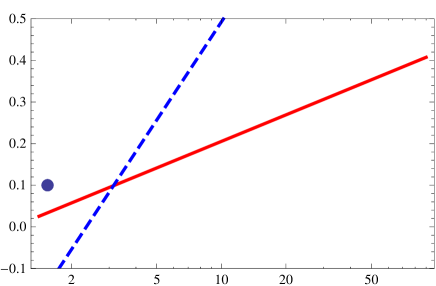
To illustrate this issue more clearly, in Fig. 1, we plot the non-perturbative form factor derived from these parameterizations, one from BLNY, and one from KN paper. If we extrapolate these parameterizations down to $Q^{2}\approx 3\textmd{GeV}^{2}$ for SIDIS at HERMES and COMPASS range, we find that $\left[\ln\left(e^{-S_{NP}}\right)\right]=-a(Q)b^{2}$ for typical value of $x\approx 0.1$ is too small to describe the data. For BLNY parameterization, even a negative value for $a(Q)$ will be found around $Q^{2}\sim 3\textmd{GeV}^{2}$, and the whole framework will break down.

The main reason of the above incompatibility is that the relative low $Q^{2}$ in current SIDIS experiments from HERMES: $Q^{2}$ is in the range of $2\sim 3\textmd{GeV}^{2}$. However, in the $b_{*}$-prescription, $1/b_{*}\sim 1/b_{max}\approx 1.5\textmd{GeV}$ is also in the similar range. The consequence is that the $Q^{2}$-dependence is mainly coming from the logarithmic dependence in the non-perturbative form factor, rather than that from the evolution itself. This has to be corrected in order to describe the SIDIS data from the CSS evolution.

On the other hand, for moderate $Q^{2}$ variations, we shall be able to understand the $Q^{2}$-dependence by directly solving the evolution equation. For example, in the Sudakov resummation formula, Eq. (50), we can, in principle, to study the $Q^{2}$ dependence by taking the structure functions at lower scale $Q_{0}$ as input, and calculate the structure function at higher $Q$ using the direct integral of the kernel from $Q_{0}$ to $Q$. That is the approach we are going to take in comparing SIDIS from HERMES/COMPASS to Drell-Yan lepton pair production. As we briefly shown in Ref. Sun:2013dya , this approach works well for $Q^{2}$ range from 2 to 100 GeV² and covers SIDIS from HERMES and COMPASS and most of the Drell-Yan processes from the fixed target experiments. Of course, for extreme high $Q$ such as $W/Z$ boson production, we have to take into account higher order corrections and back to the complete CSS resummation.

In the following, we will show that this evolution approach can describe the transverse momentum distribution in SIDIS and Drell-Yan processes up to $Q\sim 10\textmd{GeV}$. Since Drell-Yan data can also be understood from the CSS resummation with BLNY (KN) parameterization for the non-perturbative form factors, this provides a nature match between SIDIS and Drell-Yan experiments, and help us understand the TMD evolution in this particular energy range. Once we understand how this works for the unpolarized cross sections, we will extend to the Sivers single spin asymmetries in these processes.

III.5 Sun-Yuan Approach

In our calculations of the SIDIS from HERMES/COMPASS, we evolve the cross sections directly from lower to higher scale,

$$\widetilde{W}_{UU}(Q;b) = e^{-{\cal S}_{sud}(Q,Q_{0},b)}\widetilde{W}_{UU}(Q_{0};b)\ ,$$ (73)

$$\widetilde{W}_{UT}^{\alpha}(Q;b) = e^{-{\cal S}_{sud}(Q,Q_{0},b)}\widetilde{W}_{UT}^{\alpha}(Q_{0};b)\ ,$$ (74)

$$\widetilde{F}_{UU}(Q;b) = e^{-{\cal S}_{sud}(Q,Q_{0},b)}\widetilde{F}_{UU}(Q_{0};b)\ ,$$ (75)

$$\widetilde{F}_{\rm sivers}^{\alpha}(Q;b) = e^{-{\cal S}_{sud}(Q,Q_{0},b)}\widetilde{F}_{\rm sivers}^{\alpha}(Q_{0};b)\ ,$$ (76)

where the Sudakov form factor follows the above equation,

$${\cal S}_{Sud}={2C_{F}}\int_{Q_{0}}^{Q}\frac{d\bar{\mu}}{\bar{\mu}}\frac{\alpha_{s}(\bar{\mu})}{\pi}\left[\ln\left(\frac{Q^{2}}{\bar{\mu}^{2}}\right)+\ln\frac{Q_{0}^{2}b^{2}}{c_{0}^{2}}-\frac{3}{2}\right]\ .$$ (77)

The above Sudakov form factor comes from the one-loop calculations of the $A$ and $B$ coefficients of Eq. (52) in previous subsections. It has been used by Boer in previous analysis as well Boer:2001he . In the above equation, the second terms contains $b_{\perp}$ dependence which will lead to a $p_{\perp}$ broadening effects at higher $Q^{2}$ as compared to lower $Q^{2}$, whereas the first and third terms only change the normalization of the cross sections. We would like to emphasize that the Sudakov form factor is the same for the spin-average and single-spin dependent cross sections, because the associated evolution kernel is spin-independent. Moreover, both Drell-Yan and SIDIS obey the same evolution equations. The difference between the hard factors in the TMD factorization discussed in the last sections does not affect the evolution as function of $Q^{2}$.

It has been well understood that the SIDIS data from HERMES/COMPASS can be described by a Gaussian assumption for the TMDs Ref. Schweitzer:2010tt . We follow these suggestions to parameterize the lower $Q_{0}$ structure functions as,

$$\widetilde{W}_{UU}(Q_{0},b) = \sum_{q}\;e_{q}^{2}\;f_{q}(x,\mu=Q_{0})\;f_{\bar{q}}(x^{\prime},\mu=Q_{0})e^{-{g_{0}b^{2}}-{g_{0}b^{2}}}\ ,$$ (78)

$$\widetilde{W}_{UT}^{\alpha}(Q_{0},b) = \frac{-ib_{\perp}^{\alpha}M}{2}\sum_{q}\;e_{q}^{2}\;\Delta f_{q}^{\rm sivers}(x)\;f_{\bar{q}}(x^{\prime},\mu=Q_{0})e^{-(g_{0}-g_{s})b^{2}-{g_{0}b^{2}}}\ ,$$ (79)

$$\widetilde{F}_{UU}(Q_{0},b) = \sum_{q}\;e_{q}^{2}\;f_{q}(x_{B},\mu=Q_{0})\;D_{q}(z_{h},\mu=Q_{0})e^{-{g_{0}b^{2}}-{g_{h}b^{2}}/{z_{h}^{2}}}\ ,$$ (80)

$$\widetilde{F}_{\rm sivers}^{\alpha}(Q_{0},b) = \frac{ib_{\perp}^{\alpha}M}{2}\sum_{q}\;e_{q}^{2}\;\Delta f_{q}^{\rm sivers}(x)\;D_{q}(z,\mu=Q_{0})e^{-(g_{0}-g_{s})b^{2}-{g_{h}b^{2}}/{z_{h}^{2}}}\ ,$$ (81)

with $Q_{0}^{2}=2.4GeV^{2}$ chosen around HERMES kinematics, where $f$ and $D$ represent the integrated quark distribution and fragmentation functions and they are parameterized at the scale of $Q_{0}$ and we follow CT10 Lai:2010vv and DSS deFlorian:2007aj sets, respectively. In the above equations, $g_{0}$ and $g_{h}$ are chosen to be $g_{0}=0.097$ and $g_{h}=0.045$ . We have also simply assumed that all the quark flavors have the same parameters of $g_{0}$ and $g_{h}$, which shall be improved later on considering the sea quark distributions ought be different from the valence ones as demonstrated in a recent calculation Schweitzer:2012hh . The above Gaussian assumptions are simple parameterizations to describe low transverse momentum distributions. We can improve the prediction power of this simple assumption by adding a perturbative behavior at small $b_{\perp}$. However, since most of experimental data are in the low transverse momentum region, the Gaussian approximation shall be adequate to describe the majority of the data. For relative moderate transverse momentum, in particular, in high $Q^{2}$ processes, we shall improve that. The strategy of our calculations is to build match between low $Q$ SIDIS and moderate $Q$ Drell-Yan processes. Once the consistency is shown between the above evolution and the CSS resummation with BLNY (KN) parameterization of the non-perturbative form factors, it will be safe to extend to the predictions of the Sivers single spin asymmetries in Drell-Yan processes.

From the point of view of the TMD factorization, the above parameterizations correspond to the following choice for the TMD quark distribution and fragmentation functions ,

$$q(x,b_{\perp}) = f_{q}(x,Q_{0})e^{-g_{0}b^{2}}\ ,$$ (82)

$$D_{q}(z,b_{\perp}) = D_{q}(z,Q_{0})e^{-g_{h}b^{2}/z^{2}}\ ,$$ (83)

$$\tilde{f}_{1T}^{\perp(DY)}(x,b_{\perp}) = \frac{-ib_{\perp}M}{2}\Delta f^{\rm sivers}_{q}(x)\ ,$$ (84)

$$\tilde{f}_{1T}^{\perp(DIS)}(x,b_{\perp}) = \frac{ib_{\perp}M}{2}\Delta f^{\rm sivers}_{q}(x)\ ,$$ (85)

at the initial scale $Q_{0}^{2}=2.4GeV^{2}$. In terms of the Ji-Ma-Yuan scheme, the above expressions contain the soft factor contributions as well. In the Collins-11 scheme, because the soft factor has already been absorbed into the TMD quark distribution and fragmentation functions, the above expressions are just for the quark distribution and fragmentation themselves. We use the integrated quark distribution and fragmentation functions to parameterize the TMDs. The scales for the integrated distribution and fragmentation functions are set around the same scale $\mu=Q_{0}$. This is a reasonable choice, though it will introduce additional theoretical uncertainties. An aspect is that these expressions can phenomenologically reproduce the integrated distribution of the SIDIS data to a good approximation .

The opposite sign of the Sivers asymmetries between SIDIS and Drell-Yan processes is reflected by the opposite sign between $\widetilde{W}_{UT}(Q_{0})$ and $\widetilde{F}_{\rm sivers}(Q_{0})$ in the above equations. This comes from the opposite sign of the quark Sivers functions in these two processes. Comparing the above equations to those in previous sections, we find that the $\Delta f_{q}^{\rm sivers}$ parameterize the transverse-momentum moments of the quark Sivers function, $M\Delta f_{q}^{\rm sivers}=T_{F}(z,z;\mu=Q_{0})$. Again, the scale setting is similar to the above argument for the unpolarized quark distribution.

Figure 3: Multiplicity distribution as function of transverse momentum in semi-inclusive hadron production in deep inelastic scattering compared to the experimental data from HERMES collaboration at $Q^{2}=3.14$GeV² Ref. Airapetian:2012ki . These data are consistent with a Gaussian assumption in low energy scale Eq. (80).

Figure 4: Multiplicity distribution as function of transverse momentum in semi-inclusive hadron production in deep inelastic scattering compared to the experimental data from COMPASS collaboration at $Q^{2}=7.56$GeV² with moderate $x=0.1$ range of Ref. Adolph:2013stb on deuteron target. The COMPASS data, in particular, for the $p_{\perp}$ distributions, are consistent with the Sun-Yuan approach for the TMD evolution with a Gaussian assumption in low energy scale Eq. (80).

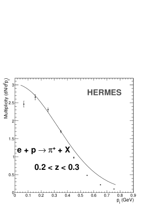
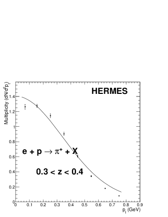
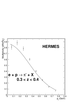
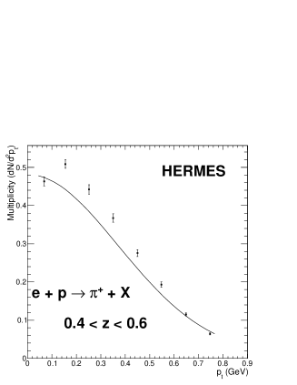
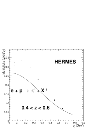
Let us first examine if the above evolution equations can describe the unpolarized cross sections in SIDIS from HERMES and COMPASS and the existing Drell-Yan lepton pair production in $pp$ collisions. Because the low $Q_{0}$ structure functions are parameterized according to HERMES data, we expect they are consistent with the experimental data from HERMES. Indeed, we show the comparisons between our calculations and the experimental data from HERMES collaboration on the charged hadron multiplicity distribution as function of the transverse momentum of final state hadron for different $z$ regions. To obtain the multiplicity distribution, we divide the differential cross section by the leading order total cross section, which contains an overall normalization uncertainty. We hope in the future that the differential cross sections for charged particles can be measured, and directly compared to the theory calculations. From these plots, we can see that the $P_{h\perp}$ distributions of the charged particle productions agree with the simple Gaussian parameterization. Since $Q^{2}=3.14GeV^{2}$ is not so different from the lower scale $Q_{0}^{2}=2.4GeV^{2}$, the evolution effects is not evident from the above comparison. We notice that the comparison at higher $z$ bin is not as good as moderate $z$ bins. This difference has also been noted in Ref. Airapetian:2012ki , where the integrated multiplicity was compared to the quark fragmentation function parameterization deFlorian:2007aj . In particular, for $\pi^{-}$, the data seems larger than the calculation based on the DSS fragmentation function in the large $z$ region. Since we have followed the DSS fragmentation functions, our predictions underestimated the experimental data at large $z$. We hope future experiments can provide more data in this region that we can constrain the theory more precisely.

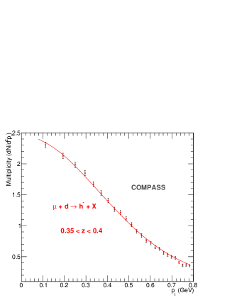
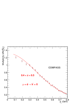
The COMPASS experiment Adolph:2013stb covers a wider range of $Q^{2}$. In particular, in the similar $x$-region, the overall $Q^{2}$ is about a factor of $2$ larger than that for HERMES experiment. Therefore, there shall be some $Q^{2}$ evolution effects in the $P_{h\perp}$ distribution for charged hadron production. In Fig. 4, we compare our predictions to the COMPASS data. Again, the multiplicity is obtained by dividing the total cross section. An additional normalization factor of 1.3 is included in these plots, which shall account for difference in the luminosity measurements in these two experiments and the possible higher order corrections. From these plots, we find an overall agreement between the theory and experiments. As we emphasized before, in this paper, we focus on the kinematic region of moderate $x$ range: $x\sim 0.1$. We do not compare our calculations with relative small-$x$ region of the COMPASS data. In the future, we hope to come back to this region, where small-$x$ effects in the transverse momentum distribution have to be taken into account.

Now, we turn to the Drell-Yan experimental data, which spans even higher $Q^{2}$ region. To calculate the transverse momentum spectrum for this process, we apply the universality of the TMD quark distributions, and the evolution equation from $Q_{0}$ scale to higher $Q$. In Fig. 5, we plot the comparisons between the theory calculations with the experimental data from E288 collaboration, where we have included an overall normalization to account for the uncertainty in the luminosity in the experiment and higher order corrections.The broadening effects for the Drell-Yan processes are well reproduced by the evolution effects of Eqs. (50,77). More comparisons between the theory calculations with the Drell-Yan data are plotted in Fig. 6. From these comparisons, we can clearly see that the evolution effects calculated from the above equations can well describe the experimental data on the unpolarized cross sections. In particular, in our calculations, the TMDs are parameterized in a Gaussian form at low scale $Q_{0}$ with a single parameter $g_{0}$, and the $Q^{2}$ dependence is calculated from the direct integral of the evolution kernel. It is almost a parameter free prediction.

As we mentioned in the Introduction, the Drell-Yan data of Figs. 5 and 6 are also extensively studied in the CSS resummation formalism. These data are actually used to constrain the associated non-perturbative form factors. To demonstrate the matching between the Sun-Yuan approach and the CSS resummation with $b_{*}$-prescription as we outlined in the Introduction, in these two plots, we also compare our calculations to the predictions from the CSS resummation with KN parameterization for the non-perturbative form factor. In these comparisons, we particularly focus on the normalized $p_{\perp}$ distribution which is crucial to estimate the single spin asymmetries in the latter calculations (Sec. V). Therefore, in the calculation, we neglect the scale dependence in the collinear parton distributions in the CSS resummation , where we have the following formula for the Drell-Yan lepton pair production,

$$\widetilde{W}_{UU}(Q;b)=e^{-{\cal S}_{pert}(Q^{2},b_{*})-S_{NP}(Q,b)}\Sigma_{q}f_{q}(z_{1},Q_{0})f_{\bar{q}}(z_{2},Q_{0})\ ,$$ (86)

where ${\cal S}_{pert}$ with $A^{(1)}$ and $B^{(1)}$ and $S_{NP}(Q,b)$ take the forms as in Eqs. (56) and (70,72), respectively. The scale of the integrated quark distributions has been fixed at $\mu^{2}=Q_{0}^{2}=2.4GeV^{2}$. These comparisons aim at a consistent check between our approach and the CSS resummation. For precise description of the experimental data, we need to implement the complete CSS resummation with the integrated quark distribution setting at the scale of $\mu=1/b_{*}$. From these comparisons, we also see that the non-perturbative form factor is the crucial part in the CSS resummation calculations for the $p_{\perp}$ spectrum for Drell-Yan processes.

Figure 5: Differential cross section for Drell-Yan lepton pair production in hadronic collisions from E288 collaboration Ito:1980ev compared to the theory predictions with TMD evolution from low energy scale $Q_{0}^{2}=2.4\textmd{GeV}^{2}$, Eqs. (73,77,78). The predictions calculated from the TMDs from Rogers et al are also shown as red curves. As a comparison, we also show predictions from the CSS resummation with the integrated quark distribution set at the scale $\mu=Q_{0}$, which gives similar results as distribution set at the scale $\mu=1/b_{*}$.

Figure 6: Same as Fig. 5 for Drell-Yan data from E605 Collaboration Moreno:1990sf .

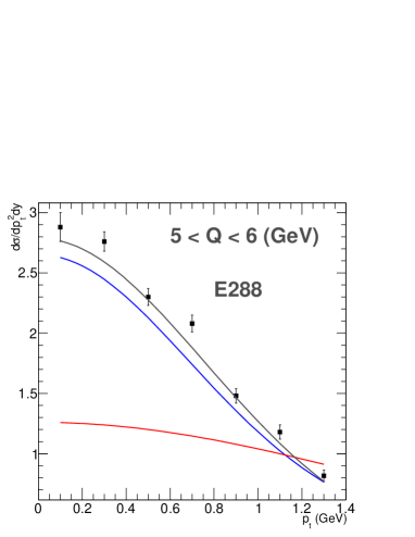
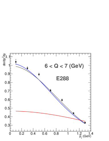
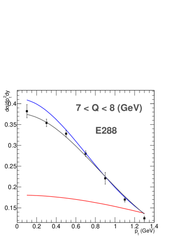
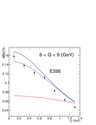
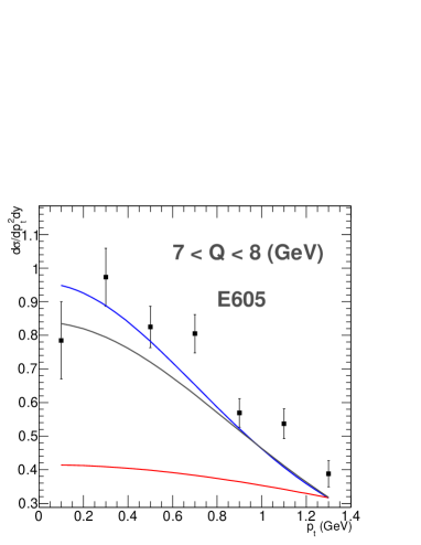
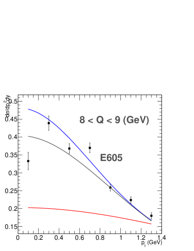
Figs. 5 and 6 provide an important evidence that we can match the different evolution formulas: at relative lower region of $Q^{2}$ we can apply the evolution equations of Eqs. (76,78); at higher region of $Q^{2}$ we apply the CSS resummation with the KN non-perturbative form factors; in the overlap region, both can be applied and present a consistent description of the experimental data. From these figures, we also observe that the CSS resummation with KN form factors describes better the experimental data than Sun-Yuan approach of the direct integral of the TMD evolution kernel. This indicates that we shall switch to the CSS resummation at high $Q^{2}$ Drell-Yan process, in particular, for $W/Z$ boson production.

The support of the matching from the above analysis encourage us to extend the above method to the Sivers single spin asymmetries in the SIDIS and Drell-Yan processes. However, the Sivers asymmetries are only observed in the SIDIS processes from HERMES and COMPASS experiments. Therefore, the measurements in the planed Drell-Yan processes will not only provide crucial test of the sign change between these two processes, but also provide unique opportunities to study the energy evolution for the spin asymmetries. This QCD dynamics shall be extensively investigated in the planed electron-ion colliders where wide coverage of $Q^{2}$ will ultimately help us understand the physics to great precision Boer:2011fh .

III.6 Rogers et al. Approach

Before we turn to the Sivers single spin asymmetry study in our calculation, in this subsection, we comment on the approach used in Rogers et al. By following Collins’ new definition for the TMD quark distributions, Rogers et al. derived an evolution equation the TMDs. However, in terms of cross section calculations, there is a simple way to understand the evolution derived by Rogers et al. For example, we can write down two equations by employing the CSS resummation with $b_{*}$-prescription,

$$\widetilde{F}_{\rm sivers}^{\alpha}(Q;b) = e^{-{\cal S}_{pert}(Q^{2},b_{*})-S_{NP}(Q,b)}\widetilde{F}_{\rm sivers}^{\alpha}(C_{1}/b,b)$$

$$\widetilde{F}_{\rm sivers}^{\alpha}(Q_{L};b) = e^{-{\cal S}_{pert}(Q_{L}^{2},b_{*})-S_{NP}(Q_{L},b)}\widetilde{F}_{\rm sivers}^{\alpha}(C_{1}/b,b)\ .$$ (87)

By combining the above two equations, we find that $F(Q)$ can be written in terms of $F(Q_{L})$,

$$\widetilde{F}_{\rm sivers}^{\alpha}(Q;b) = e^{-\left({\cal S}_{pert}(Q,b_{*})-{\cal S}_{pert}(Q_{L},b_{*})\right)}$$ (88)

$$\times e^{-\left({S}_{NP}(Q,b)-S_{NP}(Q_{L},b)\right)}$$

$$\times\widetilde{F}_{\rm sivers}^{\alpha}(Q_{L};b)\ .$$

The second exponential factor can be easily calculated $e^{-g_{2}b^{2}\ln\frac{Q}{Q_{L}}}$. It is this factor that leads to strong $Q$ dependence in the SSAs calculated in this approach in the relative low $Q$ region. However, this behavior over-predicts broadening effects in the Drell-Yan lepton pair production as compared to the experimental data. In other words, the adoption used by Rogers et al is not supported by the experimental data. In particular, the flat distribution of the transverse momentum as shown in Figs. 5 and 6 from Rogers et al. will lead to almost vanishing Sivers single spin asymmetries in the Drell-Yan processes in this transverse momentum region. Therefore, all the previous studies following this approach have to be re-examined, including, most importantly, the energy evolution for the Sivers single spin asymmetries.

IV Quark Sivers Functions from Combined Analysis of HERMES and COMPASS Data

To predict the Sivers single spin asymmetries in Drell-Yan processes, we need to constrain the quark Sivers functions from the current experimental measurements in SIDIS processes. In this section, we will perform a combined analysis of these measurements, and obtain constraints on the quark Sivers functions. A couple of comments are in order before we perform the combined fit. Our analysis of quark Sivers functions depends on the following assumptions: First, we assume that the systematics of the HERMES and COMPASS experiments are well under control. Both experiments have observed sizable Sivers asymmetries, in particular for positive charged hadrons ($\pi^{+}$ for HERMES). Second, our analysis relies on the applicability of the TMD factorization in these kinematics. Third, the experimental data are used to fit the quark Sivers functions, where we assume that it is the only contribution to the observed azimuthal asymmetries. All these important issues will be thoroughly addressed in the future SIDIS experiments, including the 12 GeV upgrade of JLab and the planed electron-ion collider. In addition, the relevant spin asymmetries in the Drell-Yan lepton pair production in $pp$ collisions in the proposed experiments shall also provide important information on the quark Sivers functions. We will discuss this in more details in Sec. V.

As we have showed in the last section, the evolution equations we derived for the moderate $Q^{2}$ range, can well describe the unpolarized differential cross sections in SIDIS and Drell-Yan processes which cover $2.5<Q^{2}<100\textmd{GeV}^{2}$. This demonstrates that the dominant evolution effects are taken into account in our derivations. In the following, we extend this approach to the Sivers single spin asymmetries in SIDIS process, and perform a combined fit to the HERMES/COMPASS data with the TMD evolution effects. Since the evolution kernel and the form of the solution is spin-independent, the structure functions at higher scale $Q$ are calculated from those from lower scale $Q_{0}$ with the Sudakov form factor, where $M=0.94\textmd{GeV}$ is a normalization scale, and we have chosen an additional parameter $g_{s}$ for transverse momentum dependence and the fragmentation part remains the same. In the following, we will fit Sivers functions by the forms:

$$\Delta f_{u}^{\rm sivers} = N_{u}x^{\alpha_{u}}(1-x)^{\beta}\frac{(\alpha_{u}+\beta)^{\alpha_{u}+\beta}}{\alpha_{u}^{\alpha_{u}}\;\beta^{\beta}}f_{u}(x,\mu=Q_{0})\ ,$$

$$\Delta f_{d}^{\rm sivers} = N_{d}x^{\alpha_{d}}(1-x)^{\beta}\frac{(\alpha_{d}+\beta)^{\alpha_{d}+\beta}}{\alpha_{d}^{\alpha_{d}}\;\beta^{\beta}}f_{d}(x,\mu=Q_{0})\ ,$$

$$\Delta f_{(\bar{u},\bar{d},s)}^{\rm sivers} = N_{(\bar{u},\bar{d},s)}x^{\alpha_{s}}(1-x)^{\beta}\frac{(\alpha_{s}+\beta)^{\alpha_{s}+\beta}}{\alpha_{s}^{\alpha_{s}}\;\beta^{\beta}}f_{(\bar{u},\bar{d},s)}(x,\mu=Q_{0})\ .$$ (89)

where $f_{u}$, $f_{d}$ and $f_{(\bar{u},\bar{d},s)}$ are integrated quark distributions at initial scale $\mu=Q_{0}$. As we have showed in the last section, that $\widetilde{F}_{UU}$ from the above equations can describe well the transverse momentum distributions in SIDIS experiments in HERMES/COMPASS kinematics. Therefore, the observed Sivers asymmetries can be used to constrain the quark Sivers functions.

In total we have ten parameters in the fit: $N_{u}$, $N_{d}$ and $N_{(\bar{u},\bar{d},s)}$ for the normalization, $\alpha_{u}$, $\alpha_{d}$, $\alpha_{s}$ and $\beta$ for $x$ and $(1-x)$ power behavior, and $g_{s}$ for the transverse momentum dependence in the Sives function. In our fit, we include the Sivers asymmetries in SIDIS, which include $\pi^{+}$, $\pi^{-}$, $\pi^{0}$, $K^{+}$, $K^{-}$ from HERMES/COMPASS, and positive and negative charged hadrons from COMPASS. We include all these in our fit . The total number of data points are 255. We use minimum $\chi^{2}$ fit by the MINUITE program package. The resulting fit gives $\chi^{2}/d.o.f=1.08$. The parameters are found to be,

$$N_{u}=0.13\pm 0.023,~{}~{}\alpha_{u}=0.81\pm 0.16,~{}~{}\beta=4.0\pm 1.2\ ,$$

$$N_{d}=-0.27\pm 0.12,~{}~{}\alpha_{d}=1.41\pm 0.28\ ,$$

$$N_{s}=0.07\pm 0.06,~{}~{}\alpha_{s}=0.58\pm 0.39\ ,$$

$$N_{\bar{u}}=-0.07\pm 0.05\ ,$$

$$N_{\bar{d}}=-0.19\pm 0.12\ ,$$

$$g_{s}=0.062\pm 0.0053\ .$$ (90)

We plot the comparisons between our fits to the experimental data in Figs. 7 and 8.

Figure 7: Comparison of our fits with the experimental data for the Sivers asymmetries as functions of $x_{B}$, $z_{h}$, and $P_{h\perp}$: HERMES data  Airapetian:2009ae .

Figure 8: Same as Fig. 7 but for COMPASS  Alekseev:2008aa ; Adolph:2012sp .

Figure 9: Moments of the quark Sivers functions $\Delta f_{q}=T_{F}(x,x)/M$ fitted to HERMES and COMPASS data: up and down quark (left) and anti-up quark (right). Upper and lower curves for the uncertainties.

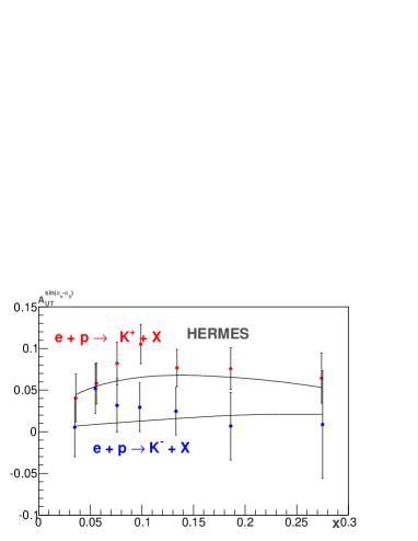
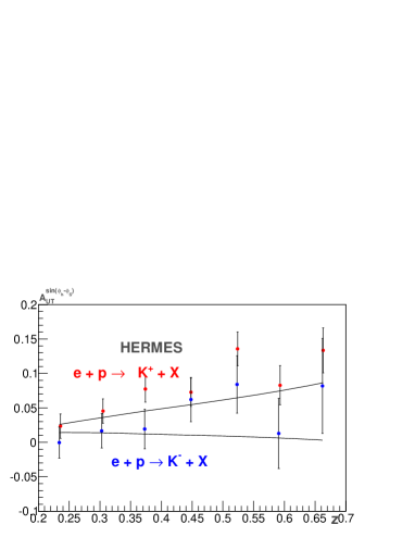
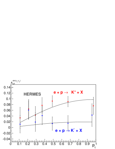
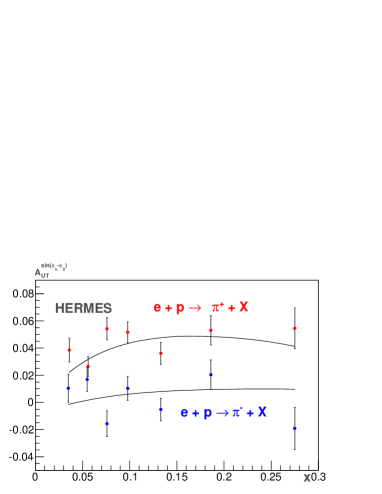
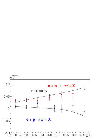
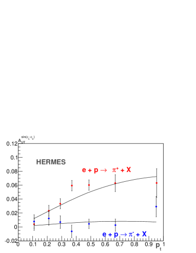
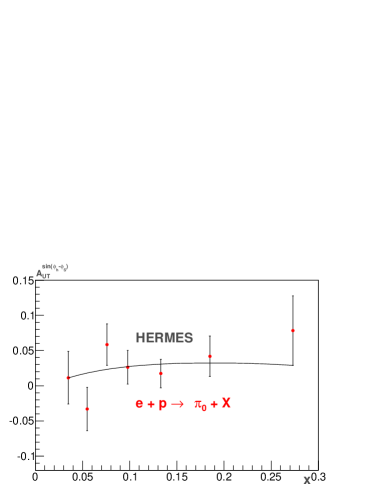
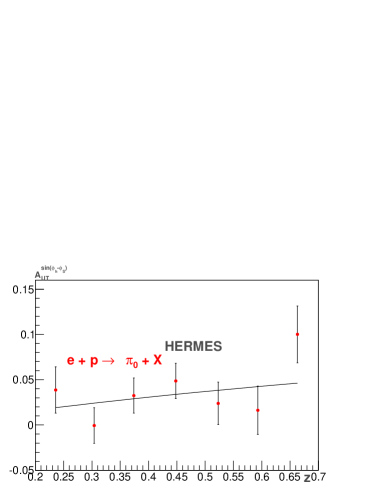
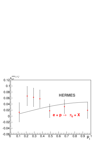
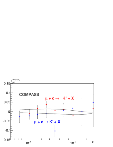
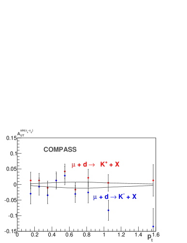
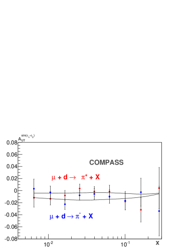
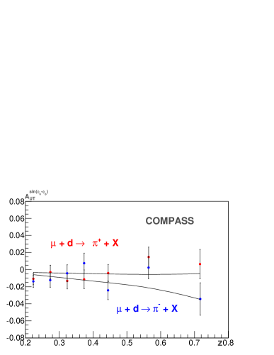
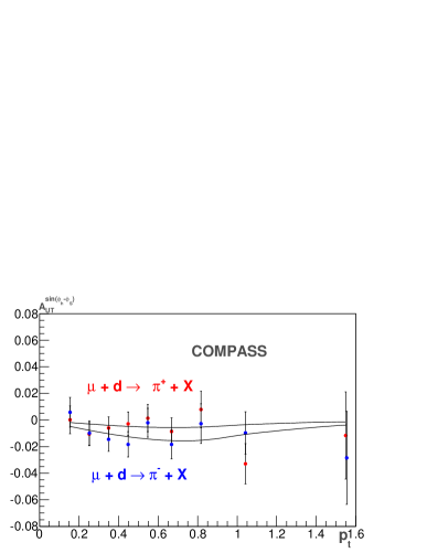
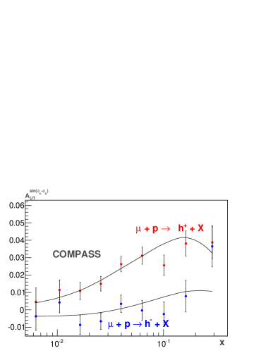
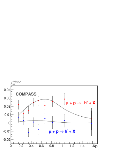
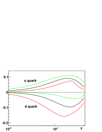
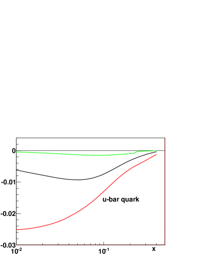
The determined Sivers functions are plotted in Fig. 9. From the above fits, we clearly see that the Sivers asymmetries in SIDIS from HERMES and COMPASS experiments have demonstrated the sizable quark Sivers functions. However, because of the experimental error bars are still large, the constraints on the quark Sivers functions are not strong enough to obtain a precise picture of the up and down quark Sivers functions. But, a number of features can be derived from the above analysis. First, the up quark Sivers function was best determined. This is because of the charge enhancement of the up quark as compared to the down quark. In other words, the SIDIS with proton target is most sensitive to the up quark contribution. Second, although the down quark Sivers was not strongly constrained from the current experimental observations, it seems that down quark Sivers function might be opposite to that of the up quark Sivers function in sign, with larger uncertainties though. Third, there is no constraints for the sea quark Sivers function at all. We need future experiments to pin down both down quark Sivers function and sea quark Sivers functions. As we mentioned above, SIDIS measurements in the 12 GeV upgrade of JLab and the planed electron-ion collider experiments, plus the Drell-Yan experiments which we will discuss in the following section, shall help us to achieve these goals.

Quark Sivers functions have been phenomenologically constrained from HERMES/COMPASS experiments by several groups in the literature Anselmino:2005an ; Anselmino:2005ea ; Anselmino:2012aa ; Bacchetta:2011gx ; Gamberg:2013kla . In the following, we briefly comment on the comparisons with these studies. First, early studies only consider the factorization of the SIDIS and the quark Sivers functions are determined by comparing the theory calculations with the experimental data without taking into account the $Q^{2}$-evolution effects. Second, Ref. Anselmino:2012aa has first started an analysis with TMD evolution following Rogers et al. approach. As we have demonstrated above, Rogers et al. approach overestimated the TMD evolution effects. The combined analysis of Ref. Anselmino:2012aa might need to be re-examined.

By comparing with previous constraints on the quark Sivers function, we notice an interesting aspect: our results agree roughly with the fits done without the TMD evolution effects. This comes from the fact that the HERMES and COMPASS experiments do not differ much on $Q^{2}$, and the evolution effects from our calculation is not so strong as naively expected. Certainly, more theoretical studies are needed to check the evolution effects.

As we emphasized above, in this paper, we focus on the quark Sivers functions in the moderate $x$ range around 0.1. this is also the region where the sizable Sivers single spin asymmetries are observed by HERMES/COMPASS experiments. For small-$x$ region quark Sivers functions, there are additional theoretical uncertainties from the TMD evolution, which has only be tested for moderate $x$ range as we showed in the last section. Therefore, the constraints for small-$x$ region quark Sivers function have to be taken a particular caution.

V Sivers SSAs in Drell-Yan and W/Z Boson Production

In this section, we present the predictions on the Sivers single spin asymmetries in Drell-Yan lepton pair production and W/Z boson production in polarized $pp$ collisions. These predictions not only serve as important base lines for the sign change tests of the Sivers asymmetry in these experimental proposals, but also provide guidelines for precision measurement of the TMD quark Sivers functions. In particular, the combination of different kinematic coverages in these experiments shall help to identify down quark and sea quark Sivers functions beyond what we can extract from the current HERMES/COMPASS experiments. Therefore, in the following, we will also highlight the opportunities in these experiments.

Since the observation of the Sivers single spin asymmetries in semi-inclusive hadron production in deep inelastic scattering process, there have been several proposals to measure the Sivers asymmetries in Drell-Yan lepton pair production in $pp$ collisions. The main focus is to observe the sign change between the Sivers asymmetries of these two processes. This is a fundamental prediction from QCD gauge theory, which is also crucial to understand the strong interaction dynamics, such as the factorization and energy evolution.

Two important issues arise when we predict the SSAs for the proposed Drell-Yan experiments. One is the flavor dependence, i.e., how precise the quark Sivers functions can be determined from the SIDIS experiments from HERMES/COMPASS collaborations. Another important issue is the energy dependence of these observables. The SIDIS experiments from HERMES and COMPASS are mainly in the relative low $Q^{2}\sim 3\textmd{GeV}^{2}$ range, whereas the Drell-Yan processes are typically range of $Q^{2}$ from $20\textmd{GeV}^{2}$ to $100\textmd{GeV}^{2}$. We have to understand the energy evolution of the Sivers spin asymmetries before we can make precise predictions.

The last few sections of this paper are dedicated to understand correctly the energy evolution of the hard processes in SIDIS and Drell-Yan lepton pair productions, including the unpolarized cross sections, and the Sivers single spin asymmetries. Our strategy has always been to test the evolution for the unpolarized cross sections before we can apply to the spin-dependent observables. We have been able to show that the energy evolution equations we used can successfully describe the transverse momentum distributions in SIDIS from HERMES/COMPASS experiments and Drell-Yan lepton pair production in fixed target experiments. HERMES/COMPASS experiments are where we observed the Sivers single spin asymmetries, whereas the Drell-Yan processes in our study are close to the kinematics of future proposed experiments to measure the Sivers single spin asymmetries. Most importantly, all these experiments (including SIDIS from HERMES/COMPASS and Drell-Yan in fixed target experiments) cover similar range of $x$. Therefore, we do not have to worry too much on additional complication involving $x$-dependence in the non-perturbative form factors in the TMD evolutions.

Let us briefly summarize our procedure to predict the SSAs in the Drell-Yan processes. We will mainly use the CSS resummation formalism in terms of the collinear parton distribution and correlation functions. The Sivers asymmetries depend on the transverse-momentum moments of the quark Sivers functions in the CSS resummation formula, which we will use the parameterization we extracted from the combined fit of the HERMES and COMPASS data from the last section. The non-perturbative form factors will follow those in Konychev-Nadolsky result, which are fitted to unpolarized Drell-Yan and W/Z boson production data. For the single spin dependent cross sections, the difference in the non-perturbative form factor $g_{s}$ was also fitted to the HERMES/COMPASS data. Since the $Q$-dependence of the non-perturbative form factors are the same for the spin-average and single-spin dependent cross sections (they obey the same evolution equation), this difference will not depend on $Q$. The fitted $g_{s}$ will be applied to the SSAs in Drell-Yan and W/Z production processes.

Before we present the detailed predictions for the Drell-Yan and W/Z processes, we would like to show that the consistency between the evolution we studied in Sec.IV and V and those from the CSS resummation with KN non-perturbative form factors. This will demonstrate that we do have a consistent match between relative low $Q$ (from which we extract the quark Sivers functions) and moderate high $Q$ (up to W/Z boson productions).

V.1 Matching SIDIS to Drell-Yan and W/Z Boson Production in $pp$ Collisions

In Sec.III, we have shown that for the unpolarized Drell-Yan cross sections from the fixed target experiments, the TMD evolution of Sun-Yuan approach is consistent with the CSS resummation with KN parameterization of the non-perturbative form factors, see Figs. 5 and 6. In this subsection, we will demonstrate that for the Sivers single spin asymmetries, both calculations will yield consistent predictions as well. This shall further strength the matching of the TMD evolution between relative low $Q$ SIDIS and moderate high $Q$ Drell-Yan processes.

The Sivers single spin asymmetries in Sun-Yuan approach are calculated with the expressions in Eqs. (73,78) for the unpolarized cross section, and equations of (74,79) for the single spin dependent cross section. We take the quark Sivers functions determined by the combined analysis in the last section. As mentioned before, the “special” universality of the quark Sivers function between Drell-Yan and SIDIS is reflected by the sign difference in Eqs. (79) and (81).

To calculate the Sivers single spin asymmetries in the CSS formalism, we follow what has been done for the unpolarized cross section of Eq. (70), and write down $\widetilde{W}_{UT}$ as

$$\widetilde{W}_{UT}(Q;b)=\left(\frac{-ib_{\perp}^{\alpha}}{2}\right)e^{-{\cal S}_{pert}(Q^{2},b_{*})-S_{NP}^{T}(Q,b)}\Sigma_{q}T_{F}^{q}(z_{1},z_{1};Q_{0})\bar{q}(z_{2},Q_{0})\ ,$$ (91)

where $S_{NP}$ follows Eqs.(70,72), and

$$S_{NP}^{T}(Q,b)=S_{NP}(Q,b)-g_{s}b^{2}$$

with $g_{s}=0.062$ fit from the HERMES and COMPASS experiments. $T_{F}(z)$ is calculated from the quark Sivers function,

$$T_{F}(z,z;\mu=Q_{0})=\int\frac{d^{2}k_{\perp}}{(2\pi)^{2}}\frac{k_{\perp}^{2}}{M}f_{1T}^{\perp(DY)}(z,k_{\perp})=M\Delta f^{\rm sivers}(z)\ ,$$ (92)

where $\Delta f^{\rm sivers}(z)$ has been determined from the combined analysis in the last section. The above identification depends on the TMD factorization, and the CSS resummation derived in Sec. II. Of course, the integrated parton correlation function, such as $T_{F}(x,x)$ depends on the scale, which is not easy to identity in the above equation. We argue that the TMD quark Sivers functions are determined at the low energy $Q_{0}$, which indicates that the moments of the quark Sivers functions calculated from the fit shall be in the similar range. Therefore, we shall be able to identify the scale for $T_{F}$ as $Q_{0}$. We notice that this will introduce some theoretical uncertainties. In particular, the scale evolution for $T_{F}$ is more complicated than that for the unpolarized quark distribution. In order to estimate the uncertainties that come from the scale setting, in the following we will make a rough estimate to see how large the scale setting affect the final results for the single spin asymmetries.

The evolution equation for $T_{F}$ has been derived in the literature. To solve this equation completely, we need input from $T_{F}(x_{1},x_{2})$ functions and $\tilde{T}_{F}$, and gluonic contributions as well. The complete solution is not available at current stage. As a first step, we take an approximate form of the splitting kernel, i.e., large $\xi$ limit. This should be relevant, in particular, in current case that the quark Sivers function mainly concentrate in the valence region. This limit has been discussed in Ref. Braun:2009mi , where the evolution can be simplified as

$$\frac{\partial}{\partial\ln\mu}T_{F}(z,z;\mu)=\frac{\alpha_{s}}{2\pi}\int\frac{dx}{x}T_{F}(x,x;\mu)\left[C_{F}\left(\frac{1+\xi^{2}}{(1-\xi)}\right)_{+}-C_{A}\delta(1-\xi)\right]\ ,$$ (93)

where $\xi=z/x$. In Ref. Braun:2009mi , it is further argued that an approximate solution of the above equation would lead to the following behavior for $T_{F}(z)$,

$$T_{F}(x,x,Q^{2})/f_{q}(x,Q^{2})\sim\left(\frac{\alpha_{s}(Q^{2})}{\alpha_{s}(Q_{0}^{2})}\right)^{2N_{c}/b_{0}}\ .$$ (94)

Since we have determined the $T_{F}$ at the scale around $\mu^{2}=2.4\textmd{GeV}^{2}$, we will be able to solve the above evolution equation numerically, by using the HOPPET program Salam:2008qg . We show the solution in Fig. 10. It is interesting to find that, indeed, in the valence region, the above approximation works for both up and down quark Sivers functions.

Figure 10: Transverse-momentum moments of the quark Sivers functions $T_{F}$ divided by the unpolarized quark distributions for up and down quarks, at the scale $\mu^{2}=Q_{0}^{2}=2.4\textmd{GeV}^{2}$, $5\textmd{GeV}^{2}$, and $10\textmd{GeV}^{2}$, respectively. $T_{F}(z,\mu)$ is obtained by solving the simplified evolution equation Eq. (93) with input parameterization at the initial scale $Q_{0}$.

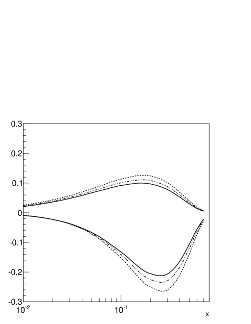
Although the scale dependence is stronger for $T_{F}$ as compared to the unpolarized quark distribution according to the evolution equation, its effects on the $p_{\perp}$ distribution from the resummation formalism may not be as strong as naively expected. This is because, in the CSS resummation formalism Eq. (55), the scale for both $T_{F}$ and $f_{q}$ is set at $\mu=1/b_{*}$ which does not change much with $Q$. To estimate this effect, we calculate the transverse momentum dependence of the Sivers single spin asymmetries in Drell-Yan lepton pair production of $Q=5.5\textmd{GeV}$ at a typical fixed target experiment with $\sqrt{S}=20\textmd{GeV}$, with three different assumptions: (1) CSS resummation with fixed scale for the parton distributions and the transverse momentum moment of the quark Sivers function $T_{F}$ as $\mu=Q_{0}$; (2) including the scale dependence in these two distributions as $\mu=c_{0}/b_{*}$; (3) Sun-Yuan approach from a direct integral of the Sudakov kernel from $Q_{0}$ to $Q$. These comparisons are plotted in Fig. 11.

Figure 11: Compare the predictions for the Sivers asymmetries in Drell-Yan lepton pair production in polarized $pp$ collisions: center of mass energy $\sqrt{S}=20\textmd{GeV}$ at $y=0$ with $Q=5.5\textmd{GeV}$: soid curve calculated with Sun-Yuan evolution, while the point curve and point slash curve are from the CSS resummation with $b_{*}$-prescription and KN paramterization of the non-perturbative form factors with fixing parton distribution scale at 2.4 GeV² and $C_{1}^{2}/b_{*}^{2}$ respectively.

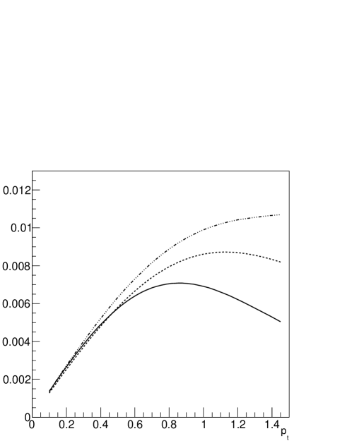
From this plot, in the low transverse momentum region, we can see that these calculations present consistent predictions for the SSAs. At higher transverse momentum, the TMD evolution of Sun-Yuan approach predicts smaller SSAs than that from the CSS resummation formalism with the two implementations (1) and (2). This comes from the Gaussian assumption of the TMDs at lower scale $Q_{0}$ which leads to more suppression of the spin asymmetry at moderate transverse momentum. However, with the CSS resummation correcting behavior for the transverse momentum distribution, this can be improved. Another point is the evolution of $T_{F}$ (implementation (2)) increases the asymmetry predictions than that without $T_{F}$ evolution. This is because for fixed scale, we have used $\mu^{2}=2.4\textmd{GeV}^{2}$, whereas at moderate transverse momentum the scale for $T_{F}$ in (2) is around $1/b_{max}$, and is smaller than $Q_{0}$. This will lead to larger $T_{F}$ contribution to the Sivers single spin asymmetries. This difference highlight the opportunities to study the QCD dynamics in this transverse momentum region, because it is sensitive to the QCD evolution. We hope in the future the Sivers single spin asymmetries can be measured in Drell-Yan process in the relative high transverse momentum region.

These two plots demonstrate that we do have a consistent picture for the Sivers single spin asymmetries in the Drell-Yan lepton pair production in the mass region of interest in the fixed target experiments. One approach (Sun-Yuan) uses the TMD evolution from SIDIS of HERMES/COMPASS to Drell-Yan processes; one approach uses the resummation formulas only for Drell-Yan processes but with the collinear correlation functions (transverse-momentum moments) extracted from HERMES/COMPASS experiments. The agreement between these two calculations shows that we understand the energy evolution effects on the Sivers single spin asymmetries.

In particular, the size and slope of the SSAs calculated from the above formulas in the low transverse momentum region agree with each other. This region is mainly determined by the ratio between the quark Sivers function and unpolarized quark distribution. The agreements indicate that the identification of $T_{F}(z,z)$ with $M\Delta f_{\rm sivers}$ is appropriate for the Sivers single spin asymmetry calculations. Of course, the difference in the relative high transverse momentum region will introduce additional theoretical uncertainties. From Fig. 11, we can estimate that the difference is around $10\%$ for the integrated asymmetries.

In the following, we will present the predictions with the CSS formalism and KN non-perturbative form factors. This approach does better job for moderate transverse momentum. In addition, it is the only approach that would predict correctly the cross section and spin asymmetries for W/Z production at RHIC.

We would like to add one more comment. From the analysis of the last section, we know that the uncertainties of the extracted quark Sivers functions from the HERMES/COMPASS experiments is not negligible. Therefore, in the following calculations, we will present the predictions with the standard one sigma uncertainty estimate for the Sivers single spin asymmetries in the Drell-Yan processes.

V.2 Drell-Yan Process in COMPASS at CERN

The COMPASS collaboration has planed to run Drell-Yan experiments in the coming years. They will use $\pi^{-}$ beam with energy 190GeV scattering on the polarized hydrogen target. The kinematic coverage can be found in the publication of Ref. compassdy .

Figure 12: Predictions for the Sivers single spin asymmetry for the Drell-Yan process at COMPASS, with $\pi^{-}$ beam of $190\textmd{GeV}$, as function of $x_{p}$. We have chosen the average $x_{\pi}\approx 0.55$ and integrate transverse momentum up to $2\textmd{GeV}$.

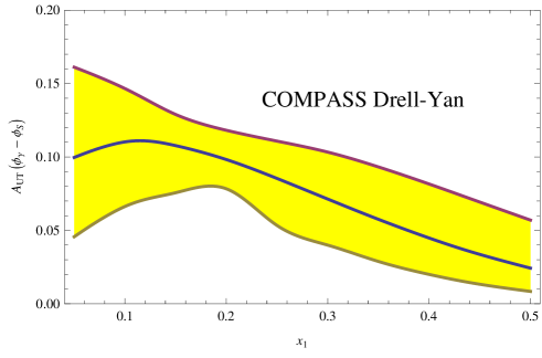
In order to make predictions for this experiment, we assume the non-perturbative form factors for $\pi^{-}N$ scattering follows the same KN parameterization. The predicted asymmetries as functions of $x_{p}$ (the momentum fraction of the proton carried by the di-lepton pair). The average $Q^{2}$ from the experimental simulation has been used in the calculations of the Sivers single spin asymmetries.

An important feature of this experiment is that the incoming $\pi^{-}$ is dominated by $\bar{u}$ and $d$ quarks from the pion, which leads to the dominant contribution from the up quark Sivers functions. The up quark Sivers function is constrained by the HERMES/COMPASS experiments. Therefore, the theory uncertainties are relative small.

There have been plan to measure the Sivers single spin asymmetries in the low mass region between $2$ and $3$ GeV for the di-lepton production in COMPASS experiment. However, in this mass region, we do have background from hadronic decays. Nevertheless, it will be interesting to measure the single spin asymmetries in these kinematics, including $J/\psi$ resonance. The latter process shall provide some information on the gluon Sivers function in the relevant kinematics.

V.3 Fermilab Fixed Target Experiments

The proposal of the polarized Drell-Yan experiments at the Fermilab contain two possible options fermilabdy : polarized beam or polarized target. Both cases can be used to measure the Sivers single spin asymmetries in the Drell-Yan lepton pair production. In the proposed experiment, the incoming beam has energy of 120GeV.

Different from the Drell-Yan experiments at COMPASS, the Fermilab proposal have proton-proton scattering. The flavor structure will be very different from that in COMPASS. This is because in the proposed kinematics, the sea quark contribution to the unpolarized cross section is not negligible. Therefore, we would expect that the sea quark Sivers functions will play an important role as well.

Figure 13: Predictions for the Sivers single spin asymmetry for the Drell-Yan process at Fermilab fixed target experiments, with proton beam of $120\textmd{GeV}$, as function of $x$ for the polarized proton: polarized beam (left) and polarized target (right).

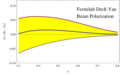
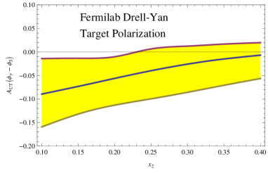
In Fig. 13, we plot our predictions for the Sivers single spin asymmetries in the Drell-Yan process at the fixed target experiment at Fermilab with polarized beam (left) or polarized target (right) options. For the beam polarization case, we show the Sivers single spin asymmetry as function of $x_{1}$ where $x_{1}$ is the momentum fraction of the polarized proton beam carried by the virtual photon in the final state, and we have chosen the average $\langle x_{2}\rangle=0.3$ from the kinematic simulation of the experimental proposal. Clearly, this experiment will mostly cover the valence region of the polarized proton, $x_{1}\geq 0.30$, which is beyond the current HERMES/COMPASS measurements. Our predictions come from the extrapolation of the function form constrained by the HERMES/COMPASS experiments. The measurements of this asymmetry in the proposed experiment shall, for the first time, investigate the Sivers asymmetries in this kinematic region.

On the other hand, for target polarization, because $x_{1}$ is still around valence region and the quark distribution is dominated by the valence up quark, the Sivers single spin asymmetry will be very sensitive to anti-up quark Sivers function. If there is no sea quark Sivers function, the asymmetry will be very small. However, with sea quark Sivers function allowed from HERMES/COMPASS experiments, we find that the Sivers asymmetry in Drell-Yan process at this experiment is relative sizable although the uncertainties are large. The predictions are shown in the right panel of Fig. 13, where average of $\langle x_{1}\rangle=0.55$ has been used in the calculations. The observation of this asymmetry will definitely signal non-zero sea quark Sivers function in this relevant kinematics.

V.4 Sivers Asymmetries in $W^{\pm}$ Production and Drell-Yan process at RHIC

Drell-Yan lepton pair production at RHIC of Brookhaven National Laboratory has been proposed for quite some time. We have presented the predictions for this experiment in Ref. Sun:2013dya . With the CSS resummation and KN parameterization for the non-perturbative form factors, we also estimated the asymmetries in Drell-Yan process at RHIC, and we obtain similar results as we showed in Sun:2013dya . In Fig. 14, we show the predictions for the Drell-Yan process in $\sqrt{S}=500\textmd{GeV}$.

Figure 14: Predictions of the Sivers single spin asymmetries for Drell-Yan process as function of rapidity at RHIC with $\sqrt{S}=500\textmd{GeV}$.

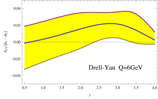
Besides the Drell-Yan process, RHIC experiments can, in principle, measure the Sivers single spin asymmetries in $W^{\pm}$ boson production in polarized proton-proton collision st $\sqrt{S}=500\textmd{GeV}$. Early calculations have emphasized the unique opportunity to test the sign change Kang:2009bp ; Metz:2010xs . In the following, we present the asymmetries calculated with the quark Sivers functions determined from HERMES/COMPASS experiments with the evolution effects taken into account.

For $W^{+}$ production, it is dominated by the Sivers up quark and anti-down quark from the polarized proton. As shown in Fig. 15, two important features can be found from our calculations: first, the prediction is much reduced as compared to the previous calculations; second, anti-down quark Sivers function also contributes significantly. However, because the uncertainties associated with the sea quark contribution is not negligible, even the sign of the Sivers asymmetries is not well constrained.

Figure 15: Predictions for the Sivers single spin asymmetries for $W^{+}$ (left) and $W^{-}$ (right) productions at RHIC with $\sqrt{S}=500\textmd{GeV}$ at mid-rapidity as functions of the transverse momenta of the vector bosons.

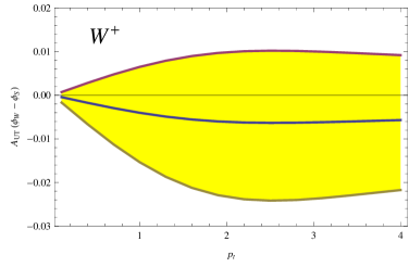
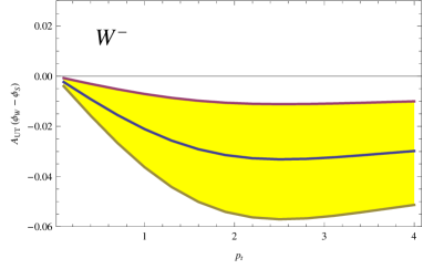
On the other hand, $W^{-}$ production is dominated by down quark and anti-up quark Sivers functions. Again, both quantities are not well constrained from HERMES/COMPASS experiments. Therefore, the observation of this asymmetry will tell us on the sea quark polarization.

We would like to emphasize that for $W/Z$ boson production, the TMD evolution directly from low scale can not describe the $p_{\perp}$ spectrum. For this, we have to use CSS resummation. The main reason is that the perturbative gluon radiation dominates the low transverse momentum $W/Z$ production, whereas the low scale TMD is not easy to generate these contributions. It may be improved by taking into account perturbative tail in the TMD quark distribution at low $Q$ scale.

VI summary and conclusion

In this paper, we have investigated the TMD evolution effects on semi-inclusive DIS and low transverse momentum Drell-Yan lepton pair production in $pp$ collisions, consistently describing both unpolarized and single transverse spin Sivers asymmetries. In particular, we have built up a framework to match SIDIS and Drell-Yan, which can cover the TMD physics with $Q^{2}$ from 2 $\textmd{GeV}^{2}$ to $10^{4}\textmd{GeV}^{2}$ (for W/Z boson production). By doing so, we constrained the transverse-momentum moments of the quark Sivers functions from the combined analysis of the HERMES/COMPASS data on the Sivers single spin asymmetries in semi-inclusive hadron production in DIS process with the TMD evolution for the spin-average and single-spin dependent differential cross sections. The TMD evolution was carefully examined against the transverse momentum distribution of unpolarized SIDIS and Drell-Yan processes in the $Q^{2}$ range from 2 to 100 $\textmd{GeV}^{2}$. Our approach agrees well with the existing experimental data.

Most importantly, we have demonstrated the matching between our evolution calculation with the well-established CSS resummation formalism with $b_{*}$-prescription and the KN parameterization of the non-perturbative form factors, for the spin-averaged cross sections, as well as the Sivers single spin asymmetries, in Drell-Yan lepton pair production in $pp$ collisions. This shows that our calculations are consistent within SIDIS from HERMES/COMPASS and Drell-Yan lepton pair production. Future experiments will provide important cross checks of our results.

A number of improvements shall follow. First, for the Drell-Yan lepton pair production, we shall include the DGLAP evolution in the CSS resummation, although the effects is not so large for low to moderate transverse momentum region. As we have shown in Fig. 11, in the relative high transverse momentum region, the DGLAP evolution is evident, and shall be able to distinguish different dynamics in the TMD evolution. Hope we will have precise experimental data in the future, which will provide unique opportunity to study the associated dynamics.

Second, our approach builds connection between relative low $Q$ hard processes to those with high $Q^{2}$ (up to $W/Z$ production): low $Q$ with direct integral of the evolution kernel; high $Q$ with CSS resummation with $b_{*}$ prescription. It will be nice to have a single framework to calculate both unpolarized and spin-dependent cross sections. To do that, we have to modify the current assumption on the non-perturbative form factors used in the literature. This will need additional research effort. We will come back to this issue later.

Third, in this paper, we only focused on the moderate $x$ range, where the $x$-dependence in the non-perturbative form factors in the CSS resummation is not so evident. In the future, we shall extend the studies to the small-$x$ region as well. For this, the HERA experiments have published data on SIDIS processes, and shall be taken into account for a global analysis.

In addition, the TMD evolutions we derived for the spin-averaged and spin-dependent cross sections can serve as guidelines for future theoretical developments. An immediate extension is to analyze the Collins asymmetries in SIDIS and di-hadron production in $e^{+}e^{-}$ annihilations. We will present a detailed calculations in a separate publication.

VII acknowledgements

We thank Z. Kang and B. Xiao for early collaboration related to Ref. Kang:2011mr . We thank A. Bressan, A. Martin, G. Schnell for communications concerning HERMES and COMPASS experimental data. We also thank Center of High Energy Physics, Peking University, for the warm host of our visits, during which this paper is finished. This work was partially supported by the U. S. Department of Energy via grant DE-AC02-05CH11231.

Appendix A Useful Fourier Transform Formulas

Let us start with the simple Fourier transform of $1/q_{\perp}^{2}$, in the $n=2-2\epsilon$ dimension,

$$\frac{\alpha_{s}}{2\pi^{2}}\int\frac{d^{n}q_{\perp}}{(2\pi)^{n}}\frac{1}{q_{\perp}^{2}}e^{iq_{\perp}\cdot b_{\perp}} = \frac{\alpha_{s}}{8\pi^{3}}\left(\frac{4}{4\pi b_{\perp}^{2}\mu^{2}}\right)^{-\epsilon}\Gamma(-\epsilon)$$ (95)

$$= \frac{\alpha_{s}}{8\pi^{3}}\left[-\frac{1}{\epsilon}+\ln\frac{c_{0}^{2}}{b_{\perp}^{2}\mu^{2}}\right]_{\rm\overline{MS}}\ ,$$

where $c_{0}=2e^{-\gamma_{E}}$ with $\gamma_{E}$ Euler constant, and the last equation is done with ${\rm\overline{MS}}$ subtraction. The leading double logarithmic term leads to the double pole contribution,

$$\frac{\alpha_{s}}{2\pi^{2}}\int\frac{d^{n}q_{\perp}}{(2\pi)^{n}}\frac{1}{q_{\perp}^{2}}\ln\frac{Q^{2}}{q_{\perp}^{2}}e^{iq_{\perp}\cdot b_{\perp}}=\frac{\alpha_{s}}{8\pi^{3}}\left(\frac{4}{4\pi b_{\perp}^{2}\mu^{2}}\right)^{-\epsilon}\lim_{\alpha\to 0}\partial_{\alpha}\left[\left(\frac{Q^{2}b_{\perp}^{2}}{4}\right)^{\alpha}\frac{\Gamma(-\epsilon-\alpha)}{\Gamma(1+\alpha)}\right]$$

$$~{}~{}~{}=\frac{\alpha_{s}}{8\pi^{3}}\left[\frac{1}{\epsilon^{2}}-\frac{1}{\epsilon}\ln\frac{Q^{2}}{\mu^{2}}+\frac{1}{2}\left(\ln\frac{Q^{2}}{\mu^{2}}\right)^{2}-\frac{1}{2}\left(\ln\frac{Q^{2}b_{\perp}^{2}}{c_{0}^{2}}\right)^{2}-\frac{\pi^{2}}{12}\right]_{\rm\overline{MS}}\ .$$ (96)

For the Sivers spin asymmetry, we have $q_{\perp}^{\beta}$ in the Fourier transform, which can be related to the above integral,

$$\int\frac{d^{n}q_{\perp}}{(2\pi)^{n}}\frac{q_{\perp}^{\beta}}{(q_{\perp}^{2})^{2}}e^{iq_{\perp}\cdot b_{\perp}} = \left(\frac{ib_{\perp}^{\beta}}{2}\right)\int\frac{d^{n}q_{\perp}}{(2\pi)^{n}}\frac{1}{q_{\perp}^{2}}e^{iq_{\perp}\cdot b_{\perp}}\ .$$ (97)

However, for the leading double logarithmic term, we have an additional term,

$$\int\frac{d^{n}q_{\perp}}{(2\pi)^{n}}\frac{q_{\perp}^{\beta}}{(q_{\perp}^{2})^{2}}\ln\frac{Q^{2}}{q_{\perp}^{2}}e^{iq_{\perp}\cdot b_{\perp}} = \left(\frac{ib_{\perp}^{\beta}}{2}\right)\left[\int\frac{d^{n}q_{\perp}}{(2\pi)^{n}}\frac{1}{q_{\perp}^{2}}\ln\frac{Q^{2}}{q_{\perp}^{2}}e^{iq_{\perp}\cdot b_{\perp}}-\int\frac{d^{n}q_{\perp}}{(2\pi)^{n}}\frac{1}{q_{\perp}^{2}}e^{iq_{\perp}\cdot b_{\perp}}\right]\ .$$ (98)

This additional term comes from the fact that the Sivers function is 2-dimension vector depending on the transverse momentum.

References

- (1) D. Boer et al., arXiv:1108.1713 [nucl-th]; A. Accardiet al., arXiv:1212.1701 [nucl-ex].
- (2) J. C. Collins and D. E. Soper, Nucl. Phys. B 193, 381 (1981) [Erratum-ibid. B 213, 545 (1983)]; Nucl. Phys. B 197, 446 (1982).
- (3) J. C. Collins, D. E. Soper and G. Sterman, Nucl. Phys. B 250, 199 (1985).
- (4) V. V. Sudakov, Sov. Phys. JETP 3, 65 (1956) [Zh. Eksp. Teor. Fiz. 30, 87 (1956)].
- (5) Y. L. Dokshitzer, D. Diakonov and S. I. Troian, Phys. Lett. B 78, 290 (1978); Phys. Lett. B 79, 269 (1978); Phys. Rept. 58, 269 (1980).
- (6) G. Parisi and R. Petronzio, Nucl. Phys. B 154, 427 (1979).
- (7) F. Landry, R. Brock, P. M. Nadolsky and C. P. Yuan, Phys. Rev. D 67, 073016 (2003); Phys. Rev. D 63, 013004 (2001).
- (8) A. V. Konychev and P. M. Nadolsky, Phys. Lett. B 633, 710 (2006).
- (9) J. -w. Qiu and X. -f. Zhang, Phys. Rev. Lett. 86, 2724 (2001) [hep-ph/0012058]; Phys. Rev. D 63, 114011 (2001) [hep-ph/0012348].
- (10) A. Kulesza, G. F. Sterman and W. Vogelsang, Phys. Rev. D 66, 014011 (2002) [hep-ph/0202251]; Phys. Rev. D 69, 014012 (2004) [hep-ph/0309264].
- (11) S. Catani, D. de Florian and M. Grazzini, Nucl. Phys. B 596, 299 (2001) [hep-ph/0008184].
- (12) S. Catani, D. de Florian, M. Grazzini and P. Nason, JHEP 0307, 028 (2003) [hep-ph/0306211].
- (13) G. Bozzi, S. Catani, D. de Florian and M. Grazzini, Phys. Lett. B 564, 65 (2003) [hep-ph/0302104]. Nucl. Phys. B 737, 73 (2006) [hep-ph/0508068]. Nucl. Phys. B 791, 1 (2008) [arXiv:0705.3887 [hep-ph]]. Nucl. Phys. B 815, 174 (2009) [arXiv:0812.2862 [hep-ph]]. Phys. Lett. B 696, 207 (2011) [arXiv:1007.2351 [hep-ph]].
- (14) X. Ji, J. P. Ma and F. Yuan, Phys. Rev. D 71, 034005 (2005); Phys. Lett. B 597, 299 (2004).
- (15) J. C. Collins and A. Metz, Phys. Rev. Lett. 93, 252001 (2004).
- (16) J.C.Collins, Foundations of Perturbative QCD, Cambridge University Press, Cambridge, 2011.
- (17) S. M. Aybat and T. C. Rogers, Phys. Rev. D 83, 114042 (2011).
- (18) S. M. Aybat, J. C. Collins, J. -W. Qiu and T. C. Rogers, Phys. Rev. D 85, 034043 (2012).
- (19) D. Boer, Nucl. Phys. B 603, 195 (2001); Nucl. Phys. B 806, 23 (2009); arXiv:1304.5387 [hep-ph].
- (20) A. Idilbi, X. Ji, J. P. Ma and F. Yuan, Phys. Rev. D 70, 074021 (2004).
- (21) Z. -B. Kang, B. -W. Xiao and F. Yuan, Phys. Rev. Lett. 107, 152002 (2011).
- (22) S. Mantry and F. Petriello, Phys. Rev. D 81, 093007 (2010) [arXiv:0911.4135 [hep-ph]]; Phys. Rev. D 83, 053007 (2011) [arXiv:1007.3773 [hep-ph]]; Phys. Rev. D 84, 014030 (2011) [arXiv:1011.0757 [hep-ph]].
- (23) T. Becher and M. Neubert, Eur. Phys. J. C 71, 1665 (2011) [arXiv:1007.4005 [hep-ph]]; T. Becher, M. Neubert and D. Wilhelm, JHEP 1202, 124 (2012) [arXiv:1109.6027 [hep-ph]]; JHEP 1305, 110 (2013) [arXiv:1212.2621 [hep-ph]].
- (24) M. G. Echevarria, A. Idilbi and I. Scimemi, JHEP 1207, 002 (2012) [arXiv:1111.4996 [hep-ph]]; arXiv:1211.1947 [hep-ph]; M. G. Echevarria, A. Idilbi, A. Schafer and I. Scimemi, arXiv:1208.1281 [hep-ph].
- (25) J. -Y. Chiu, A. Jain, D. Neill and I. Z. Rothstein, JHEP 1205, 084 (2012) [arXiv:1202.0814 [hep-ph]].
- (26) J. C. Collins and T. C. Rogers, arXiv:1210.2100 [hep-ph].
- (27) S. J. Brodsky, D. S. Hwang and I. Schmidt, Phys. Lett. B 530, 99 (2002); Nucl. Phys. B 642, 344 (2002).
- (28) J. C. Collins, Phys. Lett. B 536, 43 (2002).
- (29) A. Airapetian et al. [HERMES Collaboration], Phys. Rev. Lett. 103, 152002 (2009).
- (30) A. Airapetian et al. [HERMES Collaboration], Phys. Lett. B 693, 11 (2010).
- (31) M. Alekseev et al. [COMPASS Collaboration], Phys. Lett. B 673, 127 (2009).
- (32) C. Adolph et al. [COMPASS Collaboration], Phys. Lett. B 717, 383 (2012).
- (33) X. Qian et al. [Jefferson Lab Hall A Collaboration], Phys. Rev. Lett. 107, 072003 (2011) [arXiv:1106.0363 [nucl-ex]].
- (34) COMPASS proposal at CERN, http://wwwcompass.cern.ch/compass/proposal/compass-II_proposal/compass-II_proposal.pdf
- (35) Polarized Drell-Yan Measurements with the Fermilab Main Injector, W. Lorenzon, P.E. Reimer, et al., http://www.fnal.gov/directorate/program_planning/June2012Public/P-1027_Pol-Drell-Yan-proposal.pdf
- (36) E. C. Aschenauer, A. Bazilevsky, K. Boyle, K. O. Eyser, R. Fatemi, C. Gagliardi, M. Grosse-Perdekamp and J. Lajoie et al., arXiv:1304.0079 [nucl-ex].
- (37) W. Vogelsang and F. Yuan, Phys. Rev. D 72, 054028 (2005) [hep-ph/0507266].
- (38) J. C. Collins, A. V. Efremov, K. Goeke, M. Grosse Perdekamp, S. Menzel, B. Meredith, A. Metz and P. Schweitzer, Phys. Rev. D 73, 094023 (2006) [hep-ph/0511272].
- (39) M. Anselmino, et al., Phys. Rev. D 72, 094007 (2005) [Erratum-ibid. D 72, 099903 (2005)].
- (40) M. Anselmino, M. Boglione, J. C. Collins, U. D’Alesio, A. V. Efremov, K. Goeke, A. Kotzinian and S. Menzel et al., hep-ph/0511017.
- (41) M. Anselmino, M. Boglione, U. D’Alesio, S. Melis, F. Murgia and A. Prokudin, Phys. Rev. D 79, 054010 (2009) [arXiv:0901.3078 [hep-ph]].
- (42) Z. -B. Kang and J. -W. Qiu, Phys. Rev. D 81, 054020 (2010) [arXiv:0912.1319 [hep-ph]].
- (43) A. Bacchetta and M. Radici, Phys. Rev. Lett. 107, 212001 (2011) [arXiv:1107.5755 [hep-ph]].
- (44) L. Gamberg, Z. -B. Kang and A. Prokudin, Phys. Rev. Lett. 110, 232301 (2013) [arXiv:1302.3218 [hep-ph]].
- (45) S. M. Aybat, A. Prokudin and T. C. Rogers, Phys. Rev. Lett. 108, 242003 (2012).
- (46) M. Anselmino, M. Boglione and S. Melis, Phys. Rev. D 86, 014028 (2012).
- (47) P. Sun and F. Yuan, arXiv:1304.5037 [hep-ph].
- (48) R. Meng, F. I. Olness and D. E. Soper, Phys. Rev. D 54, 1919 (1996) [hep-ph/9511311].
- (49) P. M. Nadolsky, D. R. Stump and C. P. Yuan, Phys. Rev. D 61, 014003 (2000) [Erratum-ibid. D 64, 059903 (2001)] [hep-ph/9906280]; Phys. Rev. D 64, 114011 (2001) [hep-ph/0012261].
- (50) A. V. Efremov and O. V. Teryaev, Sov. J. Nucl. Phys. 36, 140 (1982) [Yad. Fiz. 36, 242 (1982)]; A. V. Efremov and O. V. Teryaev, Phys. Lett. B 150, 383 (1985).
- (51) J.W. Qiu and G. Sterman, Phys. Rev. Lett. 67, 2264 (1991); Nucl. Phys. B 378, 52 (1992); Phys. Rev. D 59, 014004 (1998).
- (52) X. Ji, J. W. Qiu, W. Vogelsang and F. Yuan, Phys. Rev. Lett. 97, 082002 (2006); Phys. Rev. D 73, 094017 (2006); Phys. Lett. B 638, 178 (2006); Y. Koike, W. Vogelsang and F. Yuan, Phys. Lett. B 659, 878 (2008).
- (53) A. Bacchetta, D. Boer, M. Diehl and P. J. Mulders, JHEP 0808, 023 (2008).
- (54) A. Bacchetta, U. D’Alesio, M. Diehl and C. A. Miller, Phys. Rev. D 70, 117504 (2004) [hep-ph/0410050].
- (55) W. Vogelsang and F. Yuan, Phys. Rev. D 79, 094010 (2009).
- (56) Z. B. Kang and J. W. Qiu, Phys. Rev. D 79, 016003 (2009); [arXiv:0811.3101 [hep-ph]].
- (57) J. Zhou, F. Yuan and Z. T. Liang, Phys. Rev. D 79, 114022 (2009); [arXiv:0812.4484 [hep-ph]].
- (58) V. M. Braun, A. N. Manashov and B. Pirnay, Phys. Rev. D 80, 114002 (2009). [arXiv:0909.3410 [hep-ph]].
- (59) A. Schafer and J. Zhou, Phys. Rev. D 85, 117501 (2012) [arXiv:1203.5293 [hep-ph]].
- (60) Z. -B. Kang and J. -W. Qiu, Phys. Lett. B 713, 273 (2012) [arXiv:1205.1019 [hep-ph]].
- (61) J. P. Ma and Q. Wang, Phys. Lett. B 715, 157 (2012) [arXiv:1205.0611 [hep-ph]].
- (62) A. Bacchetta, M. Diehl, K. Goeke, A. Metz, P. J. Mulders and M. Schlegel, JHEP 0702, 093 (2007).
- (63) C. Balazs and C. P. Yuan, Phys. Rev. D 56, 5558 (1997) P. M. Nadolsky, D. R. Stump and C. P. Yuan, Phys. Rev. D 61, 014003 (2000) [Erratum-ibid. D 64, 059903 (2001)]
- (64) P. Schweitzer, T. Teckentrup and A. Metz, Phys. Rev. D 81, 094019 (2010).
- (65) H. -L. Lai, M. Guzzi, J. Huston, Z. Li, P. M. Nadolsky, J. Pumplin and C. -P. Yuan, Phys. Rev. D 82, 074024 (2010) [arXiv:1007.2241 [hep-ph]].
- (66) D. de Florian, R. Sassot and M. Stratmann, Phys. Rev. D 75, 114010 (2007).
- (67) P. Schweitzer, M. Strikman and C. Weiss, JHEP 1301, 163 (2013) [arXiv:1210.1267 [hep-ph]].
- (68) A. Airapetian et al. [HERMES Collaboration], Phys. Rev. D 87, 074029 (2013).
- (69) C. Adolph et al. [COMPASS Collaboration], arXiv:1305.7317 [hep-ex].
- (70) A. S. Ito, et al., Phys. Rev. D 23, 604 (1981).
- (71) G. Moreno, C. N. Brown, W. E. Cooper, D. Finley, Y. B. Hsiung, A. M. Jonckheere, H. Jostlein and D. M. Kaplan et al., Phys. Rev. D 43, 2815 (1991).
- (72) G. P. Salam and J. Rojo, Comput. Phys. Commun. 180, 120 (2009) [arXiv:0804.3755 [hep-ph]].
- (73) Z. -B. Kang and J. -W. Qiu, Phys. Rev. Lett. 103, 172001 (2009) [arXiv:0903.3629 [hep-ph]].
- (74) A. Metz and J. Zhou, Phys. Lett. B 700, 11 (2011) [arXiv:1006.3097 [hep-ph]].