Matrix Completion in Colocated MIMO Radar:
Recoverability, Bounds & Theoretical Guarantees

Dionysios S. Kalogerias, and Athina P. Petropuluโˆ— D. S. Kalogerias and A. P. Petropulu are with the Department of Electrical & Computer Engineering, Rutgers, The State University of New Jersey, 94 Brett Rd, Piscataway, 08854, NJ, USA. e-mail: {d.kalogerias, athinap}@rutgers.eduThis work is supported by the NSF under Grant CNS-1239188, and the ONR under grant N00014-12-1-0036.
Abstract

It was recently shown that low rank matrix completion theory can be employed for designing new sampling schemes in the context of MIMO radars, which can lead to the reduction of the high volume of data typically required for accurate target detection and estimation. Employing random samplers at each reception antenna, a partially observed version of the received data matrix is formulated at the fusion center, which, under certain conditions, can be recovered using convex optimization. This paper presents the theoretical analysis regarding the performance of matrix completion in colocated MIMO radar systems, exploiting the particular structure of the data matrix. Both Uniform Linear Arrays (ULAs) and arbitrary 222-dimensional arrays are considered for transmission and reception. Especially for the ULA case, under some mild assumptions on the directions of arrival of the targets, it is explicitly shown that the coherence of the data matrix is both asymptotically and approximately optimal with respect to the number of antennas of the arrays involved and further, the data matrix is recoverable using a subset of its entries with minimal cardinality. Sufficient conditions guaranteeing low matrix coherence and consequently satisfactory matrix completion performance are also presented, including the arbitrary 222-dimensional array case.

Index Terms:
Matrix Completion, Subspace Coherence, Strong Incoherence Property, Colocated MIMO Radar, Array Processing

I Introduction

Low rank matrix completion aims at the reconstruction of a low rank data matrix using a set of limited observations of its entries. Recently, this type of estimation problems have received a lot of attention, because they arise in a variety of real world applications, such as collaborative filtering [1], sensor network positioning/localization [2] and remote sensing [3], just to name a few. Several theoretical results have been reported [4, 5, 6], and algorithms have been proposed (see, for example, [7]), providing the essential tools for solving the matrix completion problem reliably and robustly.

Most recently, matrix completion has been proposed as means for effectively reducing the volume of data required for target detection and estimation in MIMO radars [8] and more generally in array processing systems [9, 3, 10]. In [10], a collocated MIMO radar [11] scenario is considered, in which the transmission and reception antennas are organized in Uniform Linear Arrays (ULAs). Each transmission antenna transmits a narrowband waveform over a predefined carrier frequency, with the waveforms between different transmission antennas being orthogonal. At each reception antenna, after demodulation, matched filtering is performed with the transmit waveforms [10], extracting statistics and formulating a matrix (referred to here as the data matrix), which can be used by standard array processing methods for target detection and parameter estimation. For a sufficiently large number of transmission and reception antennas and a small number of targets, the data matrix is low-rank. Therefore, it can be recovered from a small number of its entries via matrix completion. This implies that, at each reception antenna, matched filtering does not need to be performed with all transmit waveforms, but rather with a small number of randomly selected ones from the waveform dictionary. The general conditions for the applicability of matrix completion were stated in [3, 10] and their validity was confirmed via simulations.

In this paper, we consider the matrix completion enabled MIMO radar system proposed in [10], and exploiting the special structure of the data matrix, we derive insightful theoretical results regarding its coherence, an important quantity closely related to its recoverability via matrix completion. Our contribution is summarized as follows:

  1. 1.

    We show that, for ULA configurations, and under mild assumptions on the Directions-Of-Arrival (DOAs) of the targets, the coherence of the data matrix is both asymptotically optimal with respect to the number of transmission and reception antennas, and nearly optimal for a sufficiently large but finite number of transmission and reception antennas.

  2. 2.

    Under common assumptions regarding the range of the pairwise differences of the target angles and the spacing of the antennas of the ULAs involved, we derive a simple sufficient condition, which essentially controls the coherence of the data matrix, as well as the rate of convergence to its optimum value. In all cases, we provide explicit and computationally tractable coherence bounds, with all results holding almost surely.

  3. 3.

    Invoking the recent theoretical results in low rank matrix completion presented in [5], we derive asymptotic bounds on the number of observations required for exact matrix completion, showing that, in fact, the matrix under consideration can be reconstructed using a subset of its entries with minimal cardinality.

  4. 4.

    We then generalize our coherence results for the more general case of arbitrary 222-dimensional transmission and reception arrays, showing that the coherence of the corresponding data can be easily and tightly bounded by simply looking at the values of the squared magnitude of a 222-dimensional complex function over a properly chosen subset of the x/y๐‘ฅ๐‘ฆx/y plane, directly related to the target angles. Essentially, by choosing a candidate pair of transmission/reception array topologies, this general result produces coherence bounds in a straightforward way, also holding true almost surely.

An important implication of the results presented in this paper is that the performance of matrix completion in colocated MIMO radar systems is completely independent of any other system design specification or target characteristic, except for the transmission/reception array topology, the target angles and possibly the wavelength of the carrier. That is, as far as matrix completion is concerned, the values of various important quantities, such as target reflection coefficients, Doppler shifts, pulse repetition intervals and the choice of the waveform dictionary are completely unconstrained. This fact makes matrix completion very appealing for reducing the number of samples needed for accurate detection and estimation in real world colocated MIMO radar systems. Also, compared to Compressive Sensing (CS) based MIMO radar, matrix completion has at least the same advantage in terms of sample reduction, justified by the strong theoretical guarantees presented here, while at the same time it avoids the angle discretization and basis mismatch issues inherent in CS-based approaches [12, 13, 14].

The paper is organized as follows. In Section II, we briefly introduce the required background in both noiseless and noisy matrix completion. We also restate the problem formulation for the MIMO radar case in a slightly more general form compared to [10]. In Section III, we present our coherence and recoverability results for ULA transmitter/receiver pairs, complete with detailed proofs and explanations. In Section IV, we present the generalization to the aforementioned coherence results for arbitrary 222-dimensional transmission/reception arrays, along with an instructive example. In Section IV, we state and prove a result for some special cases of spatial target configurations, completing our theoretical analysis. Finally, in Section V, we discuss further implications of our previously stated results and we present some simulations, validating their correctness.

II Background

II-A Noiseless Matrix Completion:
Problem Statement and Recoverability Conditions

Consider a generic complex matrix ๐Œโˆˆโ„‚N1ร—N2๐Œsuperscriptโ„‚subscript๐‘1subscript๐‘2\mathbf{M}\in\mathbb{C}^{N_{1}\times N_{2}} of rank r๐‘Ÿr, whose compact Singular Value Decomposition (SVD) is given by ๐Œ=๐”โ€‹๐šบโ€‹๐•๐‘ฏโ‰กโˆ‘iโˆˆโ„•r+ฯƒiโ€‹(๐Œ)โ€‹๐ฎiโ€‹๐ฏi๐‘ฏ๐Œ๐”๐šบsuperscript๐•๐‘ฏsubscript๐‘–superscriptsubscriptโ„•๐‘Ÿsubscript๐œŽ๐‘–๐Œsubscript๐ฎ๐‘–superscriptsubscript๐ฏ๐‘–๐‘ฏ\mathbf{M}=\mathbf{U}\boldsymbol{\Sigma}\mathbf{V}^{\boldsymbol{\mathit{H}}}\equiv\sum_{i\in\mathbb{N}_{r}^{+}}\sigma_{i}\left(\mathbf{M}\right)\mathbf{u}_{i}\mathbf{v}_{i}^{\boldsymbol{\mathit{H}}} and with column and row subspaces denoted as U๐‘ˆU and V๐‘‰V respectively, spanned by the sets {๐ฎiโˆˆโ„‚N1ร—1}iโˆˆโ„•r+subscriptsubscript๐ฎ๐‘–superscriptโ„‚subscript๐‘11๐‘–superscriptsubscriptโ„•๐‘Ÿ\left\{\mathbf{u}_{i}\in\mathbb{C}^{N_{1}\times 1}\right\}_{i\in\mathbb{N}_{r}^{+}} and {๐ฏiโˆˆโ„‚N2ร—1}iโˆˆโ„•r+subscriptsubscript๐ฏ๐‘–superscriptโ„‚subscript๐‘21๐‘–superscriptsubscriptโ„•๐‘Ÿ\left\{\mathbf{v}_{i}\in\mathbb{C}^{N_{2}\times 1}\right\}_{i\in\mathbb{N}_{r}^{+}}, respectively.

Let ๐’ซโ€‹(๐Œ)โˆˆโ„‚N1ร—N2๐’ซ๐Œsuperscriptโ„‚subscript๐‘1subscript๐‘2\mathcal{P}\left(\mathbf{M}\right)\in\mathbb{C}^{N_{1}\times N_{2}} denote an entrywise sampling of ๐Œ๐Œ\mathbf{M}. In all the analysis that follows, we will adopt the theoretical frameworks presented in [4] and [5], according to which one hopes to reconstruct ๐Œ๐Œ\mathbf{M} from ๐’ซโ€‹(๐Œ)๐’ซ๐Œ\mathcal{P}\left(\mathbf{M}\right) by solving the convex program

minimizeโ€–๐—โ€–โˆ—subjectโ€‹to๐—โ€‹(i,j)=๐Œโ€‹(i,j),โˆ€(i,j)โˆˆ๐›€,minimizesubscriptnorm๐—subjecttoformulae-sequence๐—๐‘–๐‘—๐Œ๐‘–๐‘—for-all๐‘–๐‘—๐›€\begin{array}[]{ll}\mathrm{minimize}&\left\|\mathbf{X}\right\|_{*}\\ \mathrm{subject\,to}&\mathbf{X}\left(i,j\right)=\mathbf{M}\left(i,j\right),\quad\forall\,\left(i,j\right)\in\boldsymbol{\Omega}\end{array}, (1)

where the set ๐›€๐›€\boldsymbol{\Omega} contains all matrix coordinates corresponding to the observed entries of ๐Œ๐Œ\mathbf{M} (contained in ๐’ซโ€‹(๐Œ)๐’ซ๐Œ\mathcal{P}\left(\mathbf{M}\right)) and where โ€–๐—โ€–โˆ—subscriptnorm๐—\left\|\mathbf{X}\right\|_{*} represents the nuclear norm of ๐—๐—\mathbf{X}. In the following, we will refer to (1) as the Matrix Completion (MC) problem.

Also in [4], the authors introduce the notion of subspace coherence, in order to derive specific conditions under which the solution of (1) coincides with ๐Œ๐Œ\mathbf{M}. The formal definition of subspace coherence follows, in a slightly more expanded form compared to the original definition stated in [4].

Definition 1.

(Subspace Coherence [4]) Let Uโ‰กโ„‚rโŠ†โ„‚N๐‘ˆsuperscriptโ„‚๐‘Ÿsuperscriptโ„‚๐‘U\equiv\mathbb{C}^{r}\subseteq\mathbb{C}^{N} be a subspace spanned by the set of orthonormal vectors {๐ฎiโˆˆโ„‚Nร—1}iโˆˆโ„•r+subscriptsubscript๐ฎ๐‘–superscriptโ„‚๐‘1๐‘–superscriptsubscriptโ„•๐‘Ÿ\left\{\mathbf{u}_{i}\in\mathbb{C}^{N\times 1}\right\}_{i\in\mathbb{N}_{r}^{+}}. Also, define the matrix ๐”โ‰œ[๐ฎ1โ€‹๐ฎ2โ€‹โ€ฆโ€‹๐ฎr]โˆˆโ„‚Nร—rโ‰œ๐”delimited-[]subscript๐ฎ1subscript๐ฎ2โ€ฆsubscript๐ฎ๐‘Ÿsuperscriptโ„‚๐‘๐‘Ÿ\mathbf{U}\triangleq\left[\mathbf{u}_{1}\,\mathbf{u}_{2}\,\ldots\,\mathbf{u}_{r}\right]\in\mathbb{C}^{N\times r} and let ๐Uโ‰œ๐”๐”๐‘ฏโˆˆโ„Nร—Nโ‰œsubscript๐๐‘ˆsuperscript๐”๐”๐‘ฏsuperscriptโ„๐‘๐‘\mathbf{P}_{U}\triangleq\mathbf{U}\mathbf{U}^{\boldsymbol{\mathit{H}}}\in\mathbb{R}^{N\times N} be the orthogonal projection onto U๐‘ˆU. Then, the coherence of U๐‘ˆU with respect to the standard basis {๐ži}iโˆˆโ„•N+subscriptsubscript๐ž๐‘–๐‘–superscriptsubscriptโ„•๐‘\left\{\mathbf{e}_{i}\right\}_{i\in\mathbb{N}_{N}^{+}} is defined as

ฮผโ€‹(U)๐œ‡๐‘ˆ\displaystyle\mu\left(U\right) โ‰œNrโ€‹supiโˆˆโ„•N+โ€–๐Uโ€‹๐žiโ€–22โ‰œabsent๐‘๐‘Ÿsubscriptsupremum๐‘–superscriptsubscriptโ„•๐‘superscriptsubscriptnormsubscript๐๐‘ˆsubscript๐ž๐‘–22\displaystyle\triangleq\frac{N}{r}\sup_{i\in\mathbb{N}_{N}^{+}}\left\|\mathbf{P}_{U}\mathbf{e}_{i}\right\|_{2}^{2}
โ‰กNrโ€‹supiโˆˆโ„•N+โˆ‘kโˆˆโ„•r+|๐”โ€‹(i,k)|2โˆˆ[1,Nr].absent๐‘๐‘Ÿsubscriptsupremum๐‘–superscriptsubscriptโ„•๐‘subscript๐‘˜superscriptsubscriptโ„•๐‘Ÿsuperscript๐”๐‘–๐‘˜21๐‘๐‘Ÿ\displaystyle\equiv\frac{N}{r}\sup_{i\in\mathbb{N}_{N}^{+}}\sum_{k\in\mathbb{N}_{r}^{+}}\left|\mathbf{U}\left(i,k\right)\right|^{2}\in\left[1,\dfrac{N}{r}\right]. (2)

As explained in [4], an intuitive motivation for defining subspace coherence stems from the fact that, in some sense, the singular vectors of the matrix under consideration need to be โ€œsufficiently spreadโ€, or more precisely, need to be uncorrelated to the standard basis, in order for the matrix to be fully recoverable using only a small number of its entries.

The following assumptions regarding the subspaces U๐‘ˆU and V๐‘‰V are of particular importance [4].
ย 
๐€๐ŸŽmaxโก{ฮผโ€‹(U),ฮผโ€‹(V)}โ‰คฮผ0โˆˆโ„++๐€๐ŸŽ๐œ‡๐‘ˆ๐œ‡๐‘‰subscript๐œ‡0subscriptโ„absent\mathbf{A0}\qquad\max\left\{\mu\left(U\right),\mu\left(V\right)\right\}\leq\mu_{0}\in\mathbb{R}_{++}.
ย 
๐€๐Ÿโ€–โˆ‘iโˆˆโ„•r+๐ฎiโ€‹๐ฏi๐‘ฏโ€–โˆžโ‰คฮผ1โ€‹rN1โ€‹N2,ฮผ1โˆˆโ„++formulae-sequence๐€๐Ÿsubscriptnormsubscript๐‘–superscriptsubscriptโ„•๐‘Ÿsubscript๐ฎ๐‘–superscriptsubscript๐ฏ๐‘–๐‘ฏsubscript๐œ‡1๐‘Ÿsubscript๐‘1subscript๐‘2subscript๐œ‡1subscriptโ„absent\mathbf{A1}\qquad\left\|\sum_{i\in\mathbb{N}_{r}^{+}}\mathbf{u}_{i}\mathbf{v}_{i}^{\boldsymbol{\mathit{H}}}\right\|_{\infty}\leq\mu_{1}\sqrt{\dfrac{r}{N_{1}N_{2}}},\quad\mu_{1}\in\mathbb{R}_{++}.
ย 
Indeed, if the constants ฮผ0subscript๐œ‡0\mu_{0} and ฮผ1subscript๐œ‡1\mu_{1} associated with the singular vectors of a matrix ๐Œ๐Œ\mathbf{M} are known, the following theorem holds.

Theorem 1.

(Exact MC [4]) Let ๐Œโˆˆโ„‚N1ร—N2๐Œsuperscriptโ„‚subscript๐‘1subscript๐‘2\mathbf{M}\in\mathbb{C}^{N_{1}\times N_{2}} be a matrix of rank r๐‘Ÿr obeying ๐€๐ŸŽ๐€๐ŸŽ\mathbf{A0} and ๐€๐Ÿ๐€๐Ÿ\mathbf{A1} and set Nโ‰œmaxโก{N1,N2}โ‰œ๐‘subscript๐‘1subscript๐‘2N\triangleq\max\left\{N_{1},N_{2}\right\}. Suppose we observe m๐‘šm entries of ๐Œ๐Œ\mathbf{M} with locations sampled uniformly at random. Then there exist constants C๐ถC, c๐‘c such that if

mโ‰ฅCโ€‹maxโก{ฮผ12,ฮผ01/2โ€‹ฮผ1,ฮผ0โ€‹N1/4}โ€‹Nโ€‹rโ€‹ฮฒโ€‹logโกN๐‘š๐ถsuperscriptsubscript๐œ‡12superscriptsubscript๐œ‡012subscript๐œ‡1subscript๐œ‡0superscript๐‘14๐‘๐‘Ÿ๐›ฝ๐‘m\geq C\max\left\{\mu_{1}^{2},\mu_{0}^{1/2}\mu_{1},\mu_{0}N^{1/4}\right\}Nr\beta\log N (3)

for some ฮฒ>2๐›ฝ2\beta>2, the minimizer to the program (1) is unique and equal to ๐Œ๐Œ\mathbf{M} with probability at least 1โˆ’cโ€‹Nโˆ’ฮฒ1๐‘superscript๐‘๐›ฝ1-cN^{-\beta}. For rโ‰คฮผ0โˆ’1โ€‹N1/5๐‘Ÿsuperscriptsubscript๐œ‡01superscript๐‘15r\leq\mu_{0}^{-1}N^{1/5} this estimate can be improved to

mโ‰ฅCโ€‹ฮผ0โ€‹N6/5โ€‹rโ€‹ฮฒโ€‹logโกN,๐‘š๐ถsubscript๐œ‡0superscript๐‘65๐‘Ÿ๐›ฝ๐‘m\geq C\mu_{0}N^{6/5}r\beta\log N, (4)

with the same probability of success.

If a matrix ๐Œ๐Œ\mathbf{M} obeys the assumptions ๐€๐ŸŽ๐€๐ŸŽ\mathbf{A0} and ๐€๐Ÿ๐€๐Ÿ\mathbf{A1} with parameters ฮผ0subscript๐œ‡0\mu_{0} and ฮผ1subscript๐œ‡1\mu_{1}, we will say that it obeys the incoherence property or, equivalently, that it is incoherent with parameters ฮผ0subscript๐œ‡0\mu_{0} and ฮผ1subscript๐œ‡1\mu_{1}.

In [5], the respective authors introduce a stricter assumption on the singular vectors of a generic matrix ๐Œ๐Œ\mathbf{M}, as a replacement for ๐€๐ŸŽ๐€๐ŸŽ\mathbf{A0}, enabling them to prove tighter -in fact, almost optimal- bounds on the number of observations required in order to achieve exact reconstruction of ๐Œ๐Œ\mathbf{M} by solving (1). Implicitly, they replace subspace coherence with a closely related quantity, which we will refer to as strong subspace coherence, whose definition is presented below.

Definition 2.

(Strong Subspace Coherence) Consider the hypotheses of Definition 1. Then, the strong coherence of U๐‘ˆU with respect to the standard basis {๐ži}iโˆˆโ„•N+subscriptsubscript๐ž๐‘–๐‘–superscriptsubscriptโ„•๐‘\left\{\mathbf{e}_{i}\right\}_{i\in\mathbb{N}_{N}^{+}} is defined as

ฮผsโ€‹(U)โ‰œsup(i,j)โˆˆโ„•N+ร—โ„•N+|Nrโ€‹โŸจ๐ži,๐Uโ€‹๐žjโŸฉโˆ’๐Ÿ™i=j|.โ‰œsubscript๐œ‡๐‘ ๐‘ˆsubscriptsupremum๐‘–๐‘—superscriptsubscriptโ„•๐‘superscriptsubscriptโ„•๐‘๐‘๐‘Ÿsubscript๐ž๐‘–subscript๐๐‘ˆsubscript๐ž๐‘—subscript1๐‘–๐‘—\mu_{s}\left(U\right)\triangleq\sup_{\left(i,j\right)\in\mathbb{N}_{N}^{+}\times\mathbb{N}_{N}^{+}}\left|\frac{N}{r}\left\langle\mathbf{e}_{i},\mathbf{P}_{U}\mathbf{e}_{j}\right\rangle-\mathds{1}_{i=j}\right|. (5)

Using the definition stated above, the authors in [5] essentially replace ๐€๐ŸŽ๐€๐ŸŽ\mathbf{A0} by the following assumption, concerning the singular vectors of ๐Œ๐Œ\mathbf{M}.
ย 
๐€๐Ÿmaxโก{ฮผsโ€‹(U),ฮผsโ€‹(V)}โ‰คฮผ0sr,ฮผ0sโˆˆโ„++formulae-sequence๐€๐Ÿsubscript๐œ‡๐‘ ๐‘ˆsubscript๐œ‡๐‘ ๐‘‰superscriptsubscript๐œ‡0๐‘ ๐‘Ÿsuperscriptsubscript๐œ‡0๐‘ subscriptโ„absent\mathbf{A2}\qquad\max\left\{\mu_{s}\left(U\right),\mu_{s}\left(V\right)\right\}\leq\dfrac{\mu_{0}^{s}}{\sqrt{r}},\quad\mu_{0}^{s}\in\mathbb{R}_{++}.
ย 
If ๐Œ๐Œ\mathbf{M} obeys the assumptions ๐€๐Ÿ๐€๐Ÿ\mathbf{A1} and ๐€๐Ÿ๐€๐Ÿ\mathbf{A2} with a parameter ฮผโ‰ฅmaxโก{ฮผ0s,ฮผ1}๐œ‡superscriptsubscript๐œ‡0๐‘ subscript๐œ‡1\mu\geq\max\left\{\mu_{0}^{s},\mu_{1}\right\}, we will say that it obeys the strong incoherence property or, equivalently, that it is strongly incoherent with parameter ฮผ๐œ‡\mu.

In addition, the following 222-in-111 theorem holds.

Theorem 2.

(Exact MC I & II [5]) Let ๐Œโˆˆโ„‚N1ร—N2๐Œsuperscriptโ„‚subscript๐‘1subscript๐‘2\mathbf{M}\in\mathbb{C}^{N_{1}\times N_{2}} be a matrix of rank r๐‘Ÿr obeying the strong incoherence property with parameter ฮผ๐œ‡\mu and set Nโ‰œmaxโก{N1,N2}โ‰œ๐‘subscript๐‘1subscript๐‘2N\triangleq\max\left\{N_{1},N_{2}\right\}. Suppose we observe m๐‘šm entries of ๐Œ๐Œ\mathbf{M} with locations sampled uniformly at random. Then, there exist positive numerical constants C1subscript๐ถ1C_{1} and C2subscript๐ถ2C_{2} such that if

m๐‘š\displaystyle m โ‰ฅC1โ€‹ฮผ4โ€‹Nโ€‹r2โ€‹log2โกNorabsentsubscript๐ถ1superscript๐œ‡4๐‘superscript๐‘Ÿ2superscript2๐‘or\displaystyle\geq C_{1}\mu^{4}Nr^{2}\log^{2}N\quad\text{or} (6)
m๐‘š\displaystyle m โ‰ฅC2โ€‹ฮผ2โ€‹Nโ€‹rโ€‹log6โกN,absentsubscript๐ถ2superscript๐œ‡2๐‘๐‘Ÿsuperscript6๐‘\displaystyle\geq C_{2}\mu^{2}Nr\log^{6}N, (7)

the minimizer to the program (1) is unique and equal to ๐Œ๐Œ\mathbf{M} with probability at least 1โˆ’Nโˆ’31superscript๐‘31-N^{-3}.

Further, it is easy to show that, in fact, incoherence implies strong incoherence (stated relatively informaly in [5]), as the following lemma asserts.

Lemma 1.

If a matrix ๐Œโˆˆโ„‚N1ร—N2๐Œsuperscriptโ„‚subscript๐‘1subscript๐‘2\mathbf{M}\in\mathbb{C}^{N_{1}\times N_{2}} of rank r๐‘Ÿr is incoherent with parameters ฮผ0subscript๐œ‡0\mu_{0} and ฮผ1subscript๐œ‡1\mu_{1}, it is also strongly incoherent with parameter ฮผโ‰คฮผ0โ€‹r๐œ‡subscript๐œ‡0๐‘Ÿ\mu\leq\mu_{0}\sqrt{r}.

Proof of Lemma 1.

See Appendix A.โˆŽ

II-B Noisy Matrix Completion: Stability

In the previous subsection, we have focused on cases in which the matrix observations are perfectly noiseless. Of course, in any realistic setting, these observations will be corrupted by noise, yielding the observation model (for the same generic matrix ๐Œ๐Œ\mathbf{M})

๐’ซโ€‹(๐˜)โ‰œ๐’ซโ€‹(๐Œ)+๐’ซโ€‹(๐™),โ‰œ๐’ซ๐˜๐’ซ๐Œ๐’ซ๐™\mathcal{P}\left(\mathbf{Y}\right)\triangleq\mathcal{P}\left(\mathbf{M}\right)+\mathcal{P}\left(\mathbf{Z}\right), (8)

where ๐™โˆˆโ„‚N1ร—N2๐™superscriptโ„‚subscript๐‘1subscript๐‘2\mathbf{Z}\in\mathbb{C}^{N_{1}\times N_{2}} constitutes a noise matrix with โ€–๐’ซโ€‹(๐™)โ€–Fโ‰คฮดsubscriptnorm๐’ซ๐™๐น๐›ฟ\left\|\mathcal{P}\left(\mathbf{Z}\right)\right\|_{F}\leq\delta for some known constant ฮด>0๐›ฟ0\delta>0. If ๐™๐™\mathbf{Z} is random, then ฮด๐›ฟ\delta is such that โ€–๐’ซโ€‹(๐™)โ€–Fโ‰คฮดsubscriptnorm๐’ซ๐™๐น๐›ฟ\left\|\mathcal{P}\left(\mathbf{Z}\right)\right\|_{F}\leq\delta with high probability. Then, instead of (1), the authors in [15] propose solving the program

minimizeโ€–๐—โ€–โˆ—subjectโ€‹toโ€–๐’ซโ€‹(๐—โˆ’๐˜)โ€–Fโ‰คฮด.minimizesubscriptnorm๐—subjecttosubscriptnorm๐’ซ๐—๐˜๐น๐›ฟ\begin{array}[]{ll}\mathrm{minimize}&\left\|\mathbf{X}\right\|_{*}\\ \mathrm{subject\,to}&\left\|\mathcal{P}\left(\mathbf{X}-\mathbf{Y}\right)\right\|_{F}\leq\delta\end{array}. (9)

Indeed, under the same hypotheses of Theorem 2, it can be shown that the error norm โ€–๐Œโˆ’๐Œ^โ€–Fsubscriptnorm๐Œ^๐Œ๐น\left\|\mathbf{M}-\widehat{\mathbf{M}}\right\|_{F} is bounded from above as [15]

โ€–๐Œโˆ’๐Œ^โ€–Fโ‰ค4โ€‹(2โ€‹N1โ€‹N2+m)โ€‹minโก(N1,N2)mโ€‹ฮด+2โ€‹ฮดsubscriptnorm๐Œ^๐Œ๐น42subscript๐‘1subscript๐‘2๐‘šsubscript๐‘1subscript๐‘2๐‘š๐›ฟ2๐›ฟ\left\|\mathbf{M}-\widehat{\mathbf{M}}\right\|_{F}\leq 4\sqrt{\dfrac{\left(2N_{1}N_{2}+m\right)\min\left(N_{1},N_{2}\right)}{m}}\delta+2\delta (10)

with very high probability, where ๐Œ^^๐Œ\widehat{\mathbf{M}} denotes the solution to (9). In a nutshell, as the authors in [15] aptly explain, โ€œwhen perfect noiseless recovery occurs, then matrix completion is stable vis a vis perturbationsโ€. Consequently, if ๐Œ๐Œ\mathbf{M} exhibits favorable coherence properties, both noiseless and noisy matrix completion will be more realistic. Therefore, in order to guarantee satisfactory performance for matrix completion, it suffices to study the conditions under which the coherence of ๐Œ๐Œ\mathbf{M} will be as low as possible.

II-C Matrix Completion in Colocated MIMO Radar

We consider the respective problem formulation proposed in [10] (see Subsection A of Section II in [10]). Extending the problem to the case of arbitrary 222-dimensional arrays in an obvious way [16], the matrix to be completed at the fusion center of the receiver, ๐’ซโ€‹(๐˜)๐’ซ๐˜\mathcal{P}\left(\mathbf{Y}\right), obeys the special observation model

๐˜โ‰œ๐šซ+๐™โˆˆโ„‚Mrร—Mt,โ‰œ๐˜๐šซ๐™superscriptโ„‚subscript๐‘€๐‘Ÿsubscript๐‘€๐‘ก\mathbf{Y}\triangleq\boldsymbol{\Delta}+\mathbf{Z}\in\mathbb{C}^{M_{r}\times M_{t}}, (11)

where Mrsubscript๐‘€๐‘ŸM_{r} and Mtsubscript๐‘€๐‘กM_{t} denote the numbers of reception and transmission antennas, respectively, ๐™๐™\mathbf{Z} is an interference/observation noise matrix as defined above and

๐šซโ‰œ๐—rโ€‹๐ƒ๐—t๐‘ป,โ‰œ๐šซsubscript๐—๐‘Ÿsuperscriptsubscript๐ƒ๐—๐‘ก๐‘ป\boldsymbol{\Delta}\triangleq\mathbf{X}_{r}\mathbf{D}\mathbf{X}_{t}^{\boldsymbol{T}}, (12)

where ๐—rโˆˆโ„‚Mrร—Ksubscript๐—๐‘Ÿsuperscriptโ„‚subscript๐‘€๐‘Ÿ๐พ\mathbf{X}_{r}\in\mathbb{C}^{M_{r}\times K} (respectively for ๐—tโˆˆโ„‚Mtร—Ksubscript๐—๐‘กsuperscriptโ„‚subscript๐‘€๐‘ก๐พ\mathbf{X}_{t}\in\mathbb{C}^{M_{t}\times K}) constitutes an alternant matrix defined as

๐—rsubscript๐—๐‘Ÿ\displaystyle\mathbf{X}_{r} โ‰œ[ฮณ00ฮณ10โ‹ฏฮณKโˆ’10ฮณ01ฮณ11โ‹ฏฮณKโˆ’11โ‹ฎโ‹ฎโ‹ฑโ‹ฎฮณ0Mtโˆ’1ฮณ1Mtโˆ’1โ‹ฏฮณKโˆ’1Mtโˆ’1]โˆˆโ„‚Mrร—K,โ‰œabsentmatrixsuperscriptsubscript๐›พ00superscriptsubscript๐›พ10โ‹ฏsuperscriptsubscript๐›พ๐พ10superscriptsubscript๐›พ01superscriptsubscript๐›พ11โ‹ฏsuperscriptsubscript๐›พ๐พ11โ‹ฎโ‹ฎโ‹ฑโ‹ฎsuperscriptsubscript๐›พ0subscript๐‘€๐‘ก1superscriptsubscript๐›พ1subscript๐‘€๐‘ก1โ‹ฏsuperscriptsubscript๐›พ๐พ1subscript๐‘€๐‘ก1superscriptโ„‚subscript๐‘€๐‘Ÿ๐พ\displaystyle\triangleq\begin{bmatrix}\gamma_{0}^{0}&\gamma_{1}^{0}&\cdots&\gamma_{K-1}^{0}\\ \gamma_{0}^{1}&\gamma_{1}^{1}&\cdots&\gamma_{K-1}^{1}\\ \vdots&\vdots&\ddots&\vdots\\ \gamma_{0}^{M_{t}-1}&\gamma_{1}^{M_{t}-1}&\cdots&\gamma_{K-1}^{M_{t}-1}\end{bmatrix}\in\mathbb{C}^{M_{r}\times K}, (13)

with

ฮณklsuperscriptsubscript๐›พ๐‘˜๐‘™\displaystyle\gamma_{k}^{l} โ‰œejโ€‹2โ€‹ฯ€โ€‹๐ซr๐‘ปโ€‹(l)โ€‹๐’ฏโ€‹(ฮธk),(l,k)โˆˆโ„•Mrโˆ’1ร—โ„•Kโˆ’1formulae-sequenceโ‰œabsentsuperscript๐‘’๐‘—2๐œ‹superscriptsubscript๐ซ๐‘Ÿ๐‘ป๐‘™๐’ฏsubscript๐œƒ๐‘˜๐‘™๐‘˜subscriptโ„•subscript๐‘€๐‘Ÿ1subscriptโ„•๐พ1\displaystyle\triangleq e^{j2\pi\mathbf{r}_{r}^{\boldsymbol{T}}\left(l\right)\mathcal{T}\left(\theta_{k}\right)},\quad\left(l,k\right)\in\mathbb{N}_{M_{r}-1}\times\mathbb{N}_{K-1} (14)
๐ซrโ€‹(l)subscript๐ซ๐‘Ÿ๐‘™\displaystyle\mathbf{r}_{r}\left(l\right) โ‰œ1ฮปโ€‹[xlrโ€‹ylr]๐‘ปโˆˆโ„2ร—1,lโˆˆโ„•Mrโˆ’1formulae-sequenceโ‰œabsent1๐œ†superscriptdelimited-[]superscriptsubscript๐‘ฅ๐‘™๐‘Ÿsuperscriptsubscript๐‘ฆ๐‘™๐‘Ÿ๐‘ปsuperscriptโ„21๐‘™subscriptโ„•subscript๐‘€๐‘Ÿ1\displaystyle\triangleq\dfrac{1}{\lambda}\left[x_{l}^{r}\,y_{l}^{r}\right]^{\boldsymbol{T}}\in\mathbb{R}^{2\times 1},\quad l\in\mathbb{N}_{M_{r}-1} (15)
๐’ฏโ€‹(ฮธk)๐’ฏsubscript๐œƒ๐‘˜\displaystyle\mathcal{T}\left(\theta_{k}\right) โ‰œ[cosโก(ฮธk)sinโก(ฮธk)]โˆˆโ„2ร—1,kโˆˆโ„•Kโˆ’1,formulae-sequenceโ‰œabsentmatrixsubscript๐œƒ๐‘˜subscript๐œƒ๐‘˜superscriptโ„21๐‘˜subscriptโ„•๐พ1\displaystyle\triangleq\begin{bmatrix}\cos\left(\theta_{k}\right)\\ \sin\left(\theta_{k}\right)\end{bmatrix}\in\mathbb{R}^{2\times 1},\quad k\in\mathbb{N}_{K-1}, (16)

with the sets {[xlrโ€‹ylr]๐‘ป}lโˆˆโ„•Mrโˆ’1subscriptsuperscriptdelimited-[]superscriptsubscript๐‘ฅ๐‘™๐‘Ÿsuperscriptsubscript๐‘ฆ๐‘™๐‘Ÿ๐‘ป๐‘™subscriptโ„•subscript๐‘€๐‘Ÿ1\left\{\left[x_{l}^{r}\,y_{l}^{r}\right]^{\boldsymbol{T}}\right\}_{l\in\mathbb{N}_{M_{r}-1}} and {ฮธk}kโˆˆโ„•Kโˆ’1subscriptsubscript๐œƒ๐‘˜๐‘˜subscriptโ„•๐พ1\left\{\theta_{k}\right\}_{k\in\mathbb{N}_{K-1}} containing the 222-dimensional antenna coordinates of the reception array and the target angles, respectively and ฮป๐œ†\lambda denoting the carrier wavelength utilized for the communication, and where ๐ƒโˆˆโ„‚Kร—K๐ƒsuperscriptโ„‚๐พ๐พ\mathbf{D}\in\mathbb{C}^{K\times K} constitutes a non - zero - diagonal matrix defined as

๐ƒ๐ƒ\displaystyle\mathbf{D} โ‰œdiagโ€‹([ฮถ1โ€‹ฯ1โ€‹ฮถ2โ€‹ฯ2โ€‹โ€ฆโ€‹ฮถKโ€‹ฯK]),withโ‰œabsentdiagdelimited-[]subscript๐œ1subscript๐œŒ1subscript๐œ2subscript๐œŒ2โ€ฆsubscript๐œ๐พsubscript๐œŒ๐พwith\displaystyle\triangleq\mathrm{diag}\left(\left[\zeta_{1}\rho_{1}\,\zeta_{2}\rho_{2}\,\ldots\,\zeta_{K}\rho_{K}\right]\right),\quad\text{with} (17)
ฯisubscript๐œŒ๐‘–\displaystyle\rho_{i} โ‰œexpโก(jโ€‹4โ€‹ฯ€ฮปโ€‹ฯ‘iโ€‹(qโˆ’1)โ€‹TPโ€‹R),iโˆˆโ„•Kโˆ’1,formulae-sequenceโ‰œabsent๐‘—4๐œ‹๐œ†subscriptitalic-ฯ‘๐‘–๐‘ž1subscript๐‘‡๐‘ƒ๐‘…๐‘–subscriptโ„•๐พ1\displaystyle\triangleq\exp\left(j\dfrac{4\pi}{\lambda}\vartheta_{i}\left(q-1\right)T_{PR}\right),\quad i\in\mathbb{N}_{K-1}, (18)

where the sets {ฮถk}kโˆˆโ„•Kโˆ’1subscriptsubscript๐œ๐‘˜๐‘˜subscriptโ„•๐พ1\left\{\zeta_{k}\right\}_{k\in\mathbb{N}_{K-1}} and {ฯ‘k}kโˆˆโ„•Kโˆ’1subscriptsubscriptitalic-ฯ‘๐‘˜๐‘˜subscriptโ„•๐พ1\left\{\vartheta_{k}\right\}_{k\in\mathbb{N}_{K-1}} contain the target reflection coefficients and target speeds, respectively and q๐‘žq and TPโ€‹Rsubscript๐‘‡๐‘ƒ๐‘…T_{PR} denote the pulse index and the pulse repetition interval, respectively. For the simplest ULA case (as treated in [10]),

[xlrโ€‹(t)โ€‹ylrโ€‹(t)]๐‘ปโ‰ก[0โ€‹lโ€‹drโ€‹(t)]๐‘ป,lโˆˆโ„•Mrโ€‹(t)โˆ’1,formulae-sequencesuperscriptdelimited-[]superscriptsubscript๐‘ฅ๐‘™๐‘Ÿ๐‘กsuperscriptsubscript๐‘ฆ๐‘™๐‘Ÿ๐‘ก๐‘ปsuperscriptdelimited-[]0๐‘™subscript๐‘‘๐‘Ÿ๐‘ก๐‘ป๐‘™subscriptโ„•subscript๐‘€๐‘Ÿ๐‘ก1\left[x_{l}^{r\left(t\right)}\,y_{l}^{r\left(t\right)}\right]^{\boldsymbol{T}}\equiv\left[0\,ld_{r\left(t\right)}\right]^{\boldsymbol{T}},\quad l\in\mathbb{N}_{M_{r\left(t\right)}-1}, (19)

where drโ€‹(t)subscript๐‘‘๐‘Ÿ๐‘กd_{r\left(t\right)} denotes the respective array antenna spacing, and ๐—rsubscript๐—๐‘Ÿ\mathbf{X}_{r} and ๐—tsubscript๐—๐‘ก\mathbf{X}_{t} degenerate to Vandermonde matrices.

In the next sections, we focus almost exclusively on bounding the coherence of ๐šซ๐šซ\boldsymbol{\Delta}, first for the ULA case and then for the more general arbitrary 222-dimensional array case. Also, when possible, we derive sufficient conditions under which the coherence the aforementioned matrix is small.

III Coherence and Recoverability of ๐šซ๐šซ\boldsymbol{\Delta} for
ULA Transmitter - Receiver Pairs

In this section, we present our coherence and recoverability results for the case in which ULAs are utilized for transmission and reception. In short, we prove:

  • โ€ข

    Asymptotic and approximate optimality of the coherence of ๐šซ๐šซ\boldsymbol{\Delta} with respect to the number of transmission/reception antennas and

  • โ€ข

    Near optimal recoverability of ๐šซ๐šซ\boldsymbol{\Delta} via matrix completion.

III-A Coherence of ๐šซ๐šซ\boldsymbol{\Delta}

Theorem 3.

(Coherence for ULAs) Consider a Uniform Linear Array (ULA) transmitter - receiver pair and assume that the set of target angles {ฮธk}kโˆˆโ„•Kโˆ’1subscriptsubscript๐œƒ๐‘˜๐‘˜subscriptโ„•๐พ1\left\{\theta_{k}\right\}_{k\in\mathbb{N}_{K-1}} consists of almost surely distinct members. Then, for any fixed Mtsubscript๐‘€๐‘กM_{t} and Mrsubscript๐‘€๐‘ŸM_{r}, as long as

Kโ‰คmaxiโˆˆ{t,r}โก{Miฮฒฮพiโ€‹(Mi)},๐พsubscript๐‘–๐‘ก๐‘Ÿsubscript๐‘€๐‘–subscript๐›ฝsubscript๐œ‰๐‘–subscript๐‘€๐‘–K\leq\max_{i\in\left\{t,r\right\}}\left\{\dfrac{M_{i}}{\sqrt{\beta_{\xi_{i}}\left(M_{i}\right)}}\right\}, (20)

the associated matrix ๐šซ๐šซ\boldsymbol{\Delta} obeys the assumptions ๐€๐ŸŽ๐€๐ŸŽ\mathbf{A0} and ๐€๐Ÿ๐€๐Ÿ\mathbf{A1} with

ฮผ0subscript๐œ‡0\displaystyle\mu_{0} โ‰œmaxiโˆˆ{t,r}โก{MiMiโˆ’(Kโˆ’1)โ€‹ฮฒฮพiโ€‹(Mi)}andโ‰œabsentsubscript๐‘–๐‘ก๐‘Ÿsubscript๐‘€๐‘–subscript๐‘€๐‘–๐พ1subscript๐›ฝsubscript๐œ‰๐‘–subscript๐‘€๐‘–and\displaystyle\triangleq\max_{i\in\left\{t,r\right\}}\left\{\dfrac{M_{i}}{M_{i}-\left(K-1\right)\sqrt{\beta_{\xi_{i}}\left(M_{i}\right)}}\right\}\quad\text{and} (21)
ฮผ1subscript๐œ‡1\displaystyle\mu_{1} โ‰œmaxiโˆˆ{t,r}โก{Miโ€‹KMiโˆ’(Kโˆ’1)โ€‹ฮฒฮพiโ€‹(Mi)}โ‰œabsentsubscript๐‘–๐‘ก๐‘Ÿsubscript๐‘€๐‘–๐พsubscript๐‘€๐‘–๐พ1subscript๐›ฝsubscript๐œ‰๐‘–subscript๐‘€๐‘–\displaystyle\triangleq\max_{i\in\left\{t,r\right\}}\left\{\dfrac{M_{i}\sqrt{K}}{M_{i}-\left(K-1\right)\sqrt{\beta_{\xi_{i}}\left(M_{i}\right)}}\right\} (22)

with probability 111. In the above,

ฮฒฮพkโ€‹(Mk)subscript๐›ฝsubscript๐œ‰๐‘˜subscript๐‘€๐‘˜\displaystyle\beta_{\xi_{k}}\left(M_{k}\right) โ‰œsupxโˆˆ[ฮพk,12]sin2โก(ฯ€โ€‹Mkโ€‹x)sin2โก(ฯ€โ€‹x),โ‰œabsentsubscriptsupremum๐‘ฅsubscript๐œ‰๐‘˜12superscript2๐œ‹subscript๐‘€๐‘˜๐‘ฅsuperscript2๐œ‹๐‘ฅ\displaystyle\triangleq\sup_{x\in\left[\xi_{k},\frac{1}{2}\right]}\dfrac{\sin^{2}\left(\pi M_{k}x\right)}{\sin^{2}\left(\pi x\right)}, (23)
ฮพkโ‰œmin(i,j)โˆˆโ„•Kโˆ’1ร—โ„•Kโˆ’1iโ‰ jโกgโ€‹(dkฮปโ€‹|sinโก(ฮธi)โˆ’sinโก(ฮธj)|)โ‰œsubscript๐œ‰๐‘˜subscript๐‘–๐‘—subscriptโ„•๐พ1subscriptโ„•๐พ1๐‘–๐‘—๐‘”subscript๐‘‘๐‘˜๐œ†subscript๐œƒ๐‘–subscript๐œƒ๐‘—\xi_{k}\triangleq\min_{\begin{subarray}{c}\left(i,j\right)\in\mathbb{N}_{K-1}\times\mathbb{N}_{K-1}\\ i\neq j\end{subarray}}g\left(\dfrac{d_{k}}{\lambda}\left|\sin\left(\theta_{i}\right)-\sin\left(\theta_{j}\right)\right|\right) (24)

for kโˆˆ{t,r}๐‘˜๐‘ก๐‘Ÿk\in\left\{t,r\right\} and

gโ€‹(x)โ‰œ{โŒˆxโŒ‰โˆ’x,โŒˆxโŒ‰โˆ’xโ‰ค12xโˆ’โŒŠxโŒ‹,otherwise.โ‰œ๐‘”๐‘ฅcases๐‘ฅ๐‘ฅ๐‘ฅ๐‘ฅ12๐‘ฅ๐‘ฅotherwiseg\left(x\right)\triangleq\begin{cases}\left\lceil x\right\rceil-x,&\left\lceil x\right\rceil-x\leq\dfrac{1}{2}\\ x-\left\lfloor x\right\rfloor,&\text{otherwise}\end{cases}. (25)

Further, if ฮพโ‰œminโก{ฮพr,ฮพt}โ‰ 0โ‰œ๐œ‰subscript๐œ‰๐‘Ÿsubscript๐œ‰๐‘ก0\xi\triangleq\min\left\{\xi_{r},\xi_{t}\right\}\neq 0, then, for any fixed K๐พK, as long as

miniโˆˆ{t,r}โกMiโ‰ฅKโ€‹ฮฒฮพ=๐’ชโ€‹(K),subscript๐‘–๐‘ก๐‘Ÿsubscript๐‘€๐‘–๐พsubscript๐›ฝ๐œ‰๐’ช๐พ\min_{i\in\left\{t,r\right\}}M_{i}\geq K\sqrt{\beta_{\xi}}=\mathcal{O}\left(K\right), (26)

where

ฮฒฮพsubscript๐›ฝ๐œ‰\displaystyle\beta_{\xi} โ‰œsupxโˆˆ[ฮพ,12]Mtโˆˆโ„++sin2โก(ฯ€โ€‹Mtโ€‹x)sin2โก(ฯ€โ€‹x)โ‰กsupxโˆˆ[ฮพ,12]Mrโˆˆโ„++sin2โก(ฯ€โ€‹Mrโ€‹x)sin2โก(ฯ€โ€‹x),โ‰œabsentsubscriptsupremum๐‘ฅ๐œ‰12subscript๐‘€๐‘กsubscriptโ„absentsuperscript2๐œ‹subscript๐‘€๐‘ก๐‘ฅsuperscript2๐œ‹๐‘ฅsubscriptsupremum๐‘ฅ๐œ‰12subscript๐‘€๐‘Ÿsubscriptโ„absentsuperscript2๐œ‹subscript๐‘€๐‘Ÿ๐‘ฅsuperscript2๐œ‹๐‘ฅ\displaystyle\triangleq\sup_{\begin{subarray}{c}x\in\left[\xi,\frac{1}{2}\right]\\ M_{t}\in\mathbb{R}_{++}\end{subarray}}\dfrac{\sin^{2}\left(\pi M_{t}x\right)}{\sin^{2}\left(\pi x\right)}\equiv\sup_{\begin{subarray}{c}x\in\left[\xi,\frac{1}{2}\right]\\ M_{r}\in\mathbb{R}_{++}\end{subarray}}\dfrac{\sin^{2}\left(\pi M_{r}x\right)}{\sin^{2}\left(\pi x\right)}, (27)

(21) and (22) hold replacing both ฮฒฮพtโ€‹(Mt)subscript๐›ฝsubscript๐œ‰๐‘กsubscript๐‘€๐‘ก\beta_{\xi_{t}}\left(M_{t}\right) and ฮฒฮพrโ€‹(Mr)subscript๐›ฝsubscript๐œ‰๐‘Ÿsubscript๐‘€๐‘Ÿ\beta_{\xi_{r}}\left(M_{r}\right) by the constant ฮฒฮพsubscript๐›ฝ๐œ‰\beta_{\xi} (that is, independent of both Mtsubscript๐‘€๐‘กM_{t} and Mrsubscript๐‘€๐‘ŸM_{r}). Additionally, in the limit we respect to Mtsubscript๐‘€๐‘กM_{t} and Mrsubscript๐‘€๐‘ŸM_{r}, we have

ฮผโ€‹(V)โ‰กฮผโ€‹(U)โ‰ก1,๐œ‡๐‘‰๐œ‡๐‘ˆ1\mu\left(V\right)\equiv\mu\left(U\right)\equiv 1, (28)

that is, the coherence of ๐šซ๐šซ\boldsymbol{\Delta} is asymptotically optimal. Finally, if ฮพ๐œ‰\xi is safely bounded away from zero, then, for sufficiently large Mtsubscript๐‘€๐‘กM_{t} and Mrsubscript๐‘€๐‘ŸM_{r}, it is true that

ฮผโ€‹(V)โ‰ˆฮผโ€‹(U)โ‰ˆ1.๐œ‡๐‘‰๐œ‡๐‘ˆ1\mu\left(V\right)\approx\mu\left(U\right)\approx 1. (29)

that is, the smallest possible coherence for ๐šซ๐šซ\boldsymbol{\Delta} can be approximately attained even for finite values of Mtsubscript๐‘€๐‘กM_{t} and Mrsubscript๐‘€๐‘ŸM_{r}.

Before we proceed with the proof of the theorem, let us state the following standard result, which will help us develop our arguments easily and concretely.

Theorem 4.

[17] Let ๐Œโˆˆโ„‚Nร—N๐Œsuperscriptโ„‚๐‘๐‘\mathbf{M}\in\mathbb{C}^{N\times N} be a matrix with real eigenvalues. Define

ฯ„โ‰œtrโ€‹(๐Œ)Nands2โ‰œtrโ€‹(๐Œ2)Nโˆ’ฯ„2.formulae-sequenceโ‰œ๐œtr๐Œ๐‘andโ‰œsuperscript๐‘ 2trsuperscript๐Œ2๐‘superscript๐œ2\tau\triangleq\dfrac{\mathrm{tr}\left(\mathbf{M}\right)}{N}\quad\text{and}\quad s^{2}\triangleq\dfrac{\mathrm{tr}\left(\mathbf{M}^{2}\right)}{N}-\tau^{2}. (30)

Then, it is true that

ฯ„โˆ’sโ€‹Nโˆ’1๐œ๐‘ ๐‘1\displaystyle\tau-s\sqrt{N-1} โ‰คฮปmโ€‹iโ€‹nโ€‹(๐Œ)โ‰คฯ„โˆ’sNโˆ’1andformulae-sequenceabsentsubscript๐œ†๐‘š๐‘–๐‘›๐Œ๐œ๐‘ ๐‘1and\displaystyle\leq\lambda_{min}\left(\mathbf{M}\right)\leq\tau-\dfrac{s}{\sqrt{N-1}}\quad\text{and} (31)
ฯ„+sNโˆ’1๐œ๐‘ ๐‘1\displaystyle\tau+\dfrac{s}{\sqrt{N-1}} โ‰คฮปmโ€‹aโ€‹xโ€‹(๐Œ)โ‰คฯ„+sโ€‹Nโˆ’1.absentsubscript๐œ†๐‘š๐‘Ž๐‘ฅ๐Œ๐œ๐‘ ๐‘1\displaystyle\leq\lambda_{max}\left(\mathbf{M}\right)\leq\tau+s\sqrt{N-1}. (32)

Further, equality holds on the left (right) of (31) if and only if equality holds on the left (right) of (32) if and only if the Nโˆ’1๐‘1N-1 largest (smallest) eigenvalues are equal.

Proof of Theorem 3.

In order to make it more tractable, we divide the proof into the following two subsections. In the first subsection, we present a suitable characterization of the SVD of ๐šซ๐šซ\boldsymbol{\Delta} which will come in handy in identifying the essential actions needed to be taken in order to bound its coherence. However, the methodology presented is very general and can be applied to any given rank-L๐ฟL matrix ๐Œ๐Œ\mathbf{M}, as long as it can be explicitly written as the product ๐Œ=๐Œ1โ€‹๐ƒ๐Œ2โˆˆโ„‚M1ร—M2๐Œsubscript๐Œ1subscript๐ƒ๐Œ2superscriptโ„‚subscript๐‘€1subscript๐‘€2\mathbf{M}=\mathbf{M}_{1}\mathbf{D}\mathbf{M}_{2}\in\mathbb{C}^{M_{1}\times M_{2}}, with ๐ƒโˆˆโ„‚Lร—L๐ƒsuperscriptโ„‚๐ฟ๐ฟ\mathbf{D}\in\mathbb{C}^{L\times L} being an arbitrary full rank matrix. In the second subsection, we use the results from the first, as well as the special structure of ๐šซ๐šซ\boldsymbol{\Delta} in order to derive quantitatively useful results regarding its coherence.

III-A1 Characterization of the SVD of ๐šซ๐šซ\boldsymbol{\Delta}

We would like to study the coherence of the almost surely rank-K๐พK matrix

๐šซ=๐—rโ€‹๐ƒ๐—t๐‘ปโˆˆโ„‚Mrร—Mt,๐šซsubscript๐—๐‘Ÿsuperscriptsubscript๐ƒ๐—๐‘ก๐‘ปsuperscriptโ„‚subscript๐‘€๐‘Ÿsubscript๐‘€๐‘ก\boldsymbol{\Delta}=\mathbf{X}_{r}\mathbf{D}\mathbf{X}_{t}^{\boldsymbol{T}}\in\mathbb{C}^{M_{r}\times M_{t}}, (33)

where the Vandermonde matrix ๐—rโˆˆโ„‚Mrร—Ksubscript๐—๐‘Ÿsuperscriptโ„‚subscript๐‘€๐‘Ÿ๐พ\mathbf{X}_{r}\in\mathbb{C}^{M_{r}\times K} (respectively for ๐—tโˆˆโ„‚Mtร—Ksubscript๐—๐‘กsuperscriptโ„‚subscript๐‘€๐‘ก๐พ\mathbf{X}_{t}\in\mathbb{C}^{M_{t}\times K}) is defined by the generating vector

ฮ“โ‰œ[ฮณ0โ€‹ฮณ1โ€‹โ€ฆโ€‹ฮณKโˆ’1]๐‘ปโˆˆโ„‚Kร—1,โ‰œฮ“superscriptdelimited-[]subscript๐›พ0subscript๐›พ1โ€ฆsubscript๐›พ๐พ1๐‘ปsuperscriptโ„‚๐พ1\Gamma\triangleq\left[\gamma_{0}\,\gamma_{1}\,\ldots\,\gamma_{K-1}\right]^{\boldsymbol{T}}\in\mathbb{C}^{K\times 1}, (34)

with

ฮณkโ‰œejโ€‹2โ€‹ฯ€โ€‹ฮฑkrandฮฑkrโ‰œdrโ€‹sinโก(ฮธk)ฮป,kโˆˆโ„•Kโˆ’1,formulae-sequenceโ‰œsubscript๐›พ๐‘˜superscript๐‘’๐‘—2๐œ‹superscriptsubscript๐›ผ๐‘˜๐‘Ÿandformulae-sequenceโ‰œsuperscriptsubscript๐›ผ๐‘˜๐‘Ÿsubscript๐‘‘๐‘Ÿsubscript๐œƒ๐‘˜๐œ†๐‘˜subscriptโ„•๐พ1\gamma_{k}\triangleq e^{j2\pi\alpha_{k}^{r}}\quad\text{and}\quad\alpha_{k}^{r}\triangleq\frac{d_{r}\sin\left(\theta_{k}\right)}{\lambda},\quad k\in\mathbb{N}_{K-1}, (35)

and ๐ƒโˆˆโ„‚Kร—K๐ƒsuperscriptโ„‚๐พ๐พ\mathbf{D}\in\mathbb{C}^{K\times K} is an arbitrary non - zero - diagonal matrix. Since ๐šซ๐šซ\boldsymbol{\Delta} is assumed to be of rank-K๐พK almost surely, we implicitly consider the case where the set of angles {ฮธk}kโˆˆโ„•Kโˆ’1subscriptsubscript๐œƒ๐‘˜๐‘˜subscriptโ„•๐พ1\left\{\theta_{k}\right\}_{k\in\mathbb{N}_{K-1}} consists of almost surely distinct members.

In general, the compact SVD of ๐šซ๐šซ\boldsymbol{\Delta} can be expressed as

๐šซ=๐”โ€‹๐šบโ€‹๐•๐‘ฏ,๐šซ๐”๐šบsuperscript๐•๐‘ฏ\boldsymbol{\Delta}=\mathbf{U}\boldsymbol{\Sigma}\mathbf{V}^{\boldsymbol{H}}, (36)

where ๐”โˆˆโ„‚Mrร—K๐”superscriptโ„‚subscript๐‘€๐‘Ÿ๐พ\mathbf{U}\in\mathbb{C}^{M_{r}\times K}, ๐•โˆˆโ„‚Mtร—K๐•superscriptโ„‚subscript๐‘€๐‘ก๐พ\mathbf{V}\in\mathbb{C}^{M_{t}\times K} such that ๐”๐‘ฏโ€‹๐”=๐ˆKsuperscript๐”๐‘ฏ๐”subscript๐ˆ๐พ\mathbf{U}^{\boldsymbol{H}}\mathbf{U}=\mathbf{I}_{K}, ๐•๐‘ฏโ€‹๐•=๐ˆKsuperscript๐•๐‘ฏ๐•subscript๐ˆ๐พ\mathbf{V}^{\boldsymbol{H}}\mathbf{V}=\mathbf{I}_{K} and ๐šบโˆˆโ„Kร—K๐šบsuperscriptโ„๐พ๐พ\boldsymbol{\Sigma}\in\mathbb{R}^{K\times K} constitutes a diagonal matrix containing the (non zero) singular values of ๐šซ๐šซ\boldsymbol{\Delta}.

Respectively for ๐—tsubscript๐—๐‘ก\mathbf{X}_{t}, consider the thin QR decomposition of ๐—rsubscript๐—๐‘Ÿ\mathbf{X}_{r} given by ๐—r=๐•rโ€‹๐€rsubscript๐—๐‘Ÿsubscript๐•๐‘Ÿsubscript๐€๐‘Ÿ\mathbf{X}_{r}=\mathbf{V}_{r}\mathbf{A}_{r}, where ๐•rโˆˆโ„‚Mrร—Ksubscript๐•๐‘Ÿsuperscriptโ„‚subscript๐‘€๐‘Ÿ๐พ\mathbf{V}_{r}\in\mathbb{C}^{M_{r}\times K} is such that ๐•r๐‘ฏโ€‹๐•rโ‰ก๐ˆKsuperscriptsubscript๐•๐‘Ÿ๐‘ฏsubscript๐•๐‘Ÿsubscript๐ˆ๐พ\mathbf{V}_{r}^{\boldsymbol{\mathit{H}}}\mathbf{V}_{r}\equiv\mathbf{I}_{K} and ๐€rโˆˆโ„‚Kร—Ksubscript๐€๐‘Ÿsuperscriptโ„‚๐พ๐พ\mathbf{A}_{r}\in\mathbb{C}^{K\times K} constitutes an upper triangular matrix. Then, ๐šซ=๐•rโ€‹๐€rโ€‹๐ƒ๐€t๐‘ปโ€‹๐•t๐‘ป๐šซsubscript๐•๐‘Ÿsubscript๐€๐‘Ÿsuperscriptsubscript๐ƒ๐€๐‘ก๐‘ปsuperscriptsubscript๐•๐‘ก๐‘ป\boldsymbol{\Delta}=\mathbf{V}_{r}\mathbf{A}_{r}\mathbf{D}\mathbf{A}_{t}^{\boldsymbol{\mathit{T}}}\mathbf{V}_{t}^{\boldsymbol{\mathit{T}}} and since the matrix ๐€rโ€‹๐ƒ๐€t๐‘ปโˆˆโ„‚Kร—Ksubscript๐€๐‘Ÿsuperscriptsubscript๐ƒ๐€๐‘ก๐‘ปsuperscriptโ„‚๐พ๐พ\mathbf{A}_{r}\mathbf{D}\mathbf{A}_{t}^{\boldsymbol{\mathit{T}}}\in\mathbb{C}^{K\times K} is almost surely of full rank by definition, its SVD is given by ๐€rโ€‹๐ƒ๐€t๐‘ป=๐rโ€‹๐šฒโ€‹๐t๐‘ฏsubscript๐€๐‘Ÿsuperscriptsubscript๐ƒ๐€๐‘ก๐‘ปsubscript๐๐‘Ÿ๐šฒsuperscriptsubscript๐๐‘ก๐‘ฏ\mathbf{A}_{r}\mathbf{D}\mathbf{A}_{t}^{\boldsymbol{\mathit{T}}}=\mathbf{Q}_{r}\boldsymbol{\Lambda}\mathbf{Q}_{t}^{\boldsymbol{\mathit{H}}}, where ๐rโˆˆโ„‚Kร—Ksubscript๐๐‘Ÿsuperscriptโ„‚๐พ๐พ\mathbf{Q}_{r}\in\mathbb{C}^{K\times K} is such that ๐rโ€‹๐r๐‘ฏ=๐r๐‘ฏโ€‹๐rโ‰ก๐ˆKsubscript๐๐‘Ÿsuperscriptsubscript๐๐‘Ÿ๐‘ฏsuperscriptsubscript๐๐‘Ÿ๐‘ฏsubscript๐๐‘Ÿsubscript๐ˆ๐พ\mathbf{Q}_{r}\mathbf{Q}_{r}^{\boldsymbol{\mathit{H}}}=\mathbf{Q}_{r}^{\boldsymbol{\mathit{H}}}\mathbf{Q}_{r}\equiv\mathbf{I}_{K} (respectively for ๐rsubscript๐๐‘Ÿ\mathbf{Q}_{r}) and ๐šฒโˆˆโ„Kร—K๐šฒsuperscriptโ„๐พ๐พ\boldsymbol{\Lambda}\in\mathbb{R}^{K\times K} is non - zero - diagonal, containing the singular values of ๐€rโ€‹๐ƒ๐€t๐‘ปsubscript๐€๐‘Ÿsuperscriptsubscript๐ƒ๐€๐‘ก๐‘ป\mathbf{A}_{r}\mathbf{D}\mathbf{A}_{t}^{\boldsymbol{\mathit{T}}}. Thus, we arrive at the expression

๐šซ=๐•rโ€‹๐rโ€‹๐šฒโ€‹๐t๐‘ฏโ€‹๐•t๐‘ปโ‰ก๐•rโ€‹๐rโ€‹๐šฒโ€‹(๐•tโˆ—โ€‹๐t)๐‘ฏ,๐šซsubscript๐•๐‘Ÿsubscript๐๐‘Ÿ๐šฒsuperscriptsubscript๐๐‘ก๐‘ฏsuperscriptsubscript๐•๐‘ก๐‘ปsubscript๐•๐‘Ÿsubscript๐๐‘Ÿ๐šฒsuperscriptsuperscriptsubscript๐•๐‘กsubscript๐๐‘ก๐‘ฏ\boldsymbol{\Delta}=\mathbf{V}_{r}\mathbf{Q}_{r}\boldsymbol{\Lambda}\mathbf{Q}_{t}^{\boldsymbol{\mathit{H}}}\mathbf{V}_{t}^{\boldsymbol{\mathit{T}}}\equiv\mathbf{V}_{r}\mathbf{Q}_{r}\boldsymbol{\Lambda}\left(\mathbf{V}_{t}^{*}\mathbf{Q}_{t}\right)^{\boldsymbol{\mathit{H}}}, (37)

which constitutes a valid SVD of ๐šซ๐šซ\boldsymbol{\Delta}, since (๐•rโ€‹๐r)๐‘ฏโ€‹๐•rโ€‹๐rโ‰ก๐ˆKsuperscriptsubscript๐•๐‘Ÿsubscript๐๐‘Ÿ๐‘ฏsubscript๐•๐‘Ÿsubscript๐๐‘Ÿsubscript๐ˆ๐พ\left(\mathbf{V}_{r}\mathbf{Q}_{r}\right)^{\boldsymbol{\mathit{H}}}\mathbf{V}_{r}\mathbf{Q}_{r}\equiv\mathbf{I}_{K} and (๐•tโˆ—โ€‹๐t)๐‘ฏโ€‹๐•tโˆ—โ€‹๐tโ‰ก๐ˆKsuperscriptsuperscriptsubscript๐•๐‘กsubscript๐๐‘ก๐‘ฏsuperscriptsubscript๐•๐‘กsubscript๐๐‘กsubscript๐ˆ๐พ\left(\mathbf{V}_{t}^{*}\mathbf{Q}_{t}\right)^{\boldsymbol{\mathit{H}}}\mathbf{V}_{t}^{*}\mathbf{Q}_{t}\equiv\mathbf{I}_{K} and consequently, by the uniqueness of the singular values of a matrix, ๐šฒโ‰ก๐šบ๐šฒ๐šบ\boldsymbol{\Lambda}\equiv\boldsymbol{\Sigma}. Therefore, we can set ๐”=๐•rโ€‹๐r๐”subscript๐•๐‘Ÿsubscript๐๐‘Ÿ\mathbf{U}=\mathbf{V}_{r}\mathbf{Q}_{r} and ๐•=๐•tโˆ—โ€‹๐t๐•superscriptsubscript๐•๐‘กsubscript๐๐‘ก\mathbf{V}=\mathbf{V}_{t}^{*}\mathbf{Q}_{t}.

If ๐•riโˆˆโ„‚1ร—Ksuperscriptsubscript๐•๐‘Ÿ๐‘–superscriptโ„‚1๐พ\mathbf{V}_{r}^{i}\in\mathbb{C}^{1\times K} and ๐—riโˆˆโ„‚1ร—K,iโˆˆโ„•Mr+formulae-sequencesuperscriptsubscript๐—๐‘Ÿ๐‘–superscriptโ„‚1๐พ๐‘–superscriptsubscriptโ„•subscript๐‘€๐‘Ÿ\mathbf{X}_{r}^{i}\in\mathbb{C}^{1\times K},i\in\mathbb{N}_{M_{r}}^{+} denote the i๐‘–i-th row of ๐•rsubscript๐•๐‘Ÿ\mathbf{V}_{r} and ๐—rsubscript๐—๐‘Ÿ\mathbf{X}_{r}, respectively, it holds that

ฮผโ€‹(U)๐œ‡๐‘ˆ\displaystyle\mu\left(U\right) =MrKโ€‹supiโˆˆโ„•N+โ€–๐•riโ€‹๐rโ€–22absentsubscript๐‘€๐‘Ÿ๐พsubscriptsupremum๐‘–superscriptsubscriptโ„•๐‘superscriptsubscriptnormsuperscriptsubscript๐•๐‘Ÿ๐‘–subscript๐๐‘Ÿ22\displaystyle=\frac{M_{r}}{K}\sup_{i\in\mathbb{N}_{N}^{+}}\left\|\mathbf{V}_{r}^{i}\mathbf{Q}_{r}\right\|_{2}^{2}
โ‰กMrKโ€‹supiโˆˆโ„•N+โ€–๐•riโ€–22absentsubscript๐‘€๐‘Ÿ๐พsubscriptsupremum๐‘–superscriptsubscriptโ„•๐‘superscriptsubscriptnormsuperscriptsubscript๐•๐‘Ÿ๐‘–22\displaystyle\equiv\frac{M_{r}}{K}\sup_{i\in\mathbb{N}_{N}^{+}}\left\|\mathbf{V}_{r}^{i}\right\|_{2}^{2} (38)
=MrKโ€‹supiโˆˆโ„•N+โ€–๐—riโ€‹๐€rโˆ’1โ€–22absentsubscript๐‘€๐‘Ÿ๐พsubscriptsupremum๐‘–superscriptsubscriptโ„•๐‘superscriptsubscriptnormsuperscriptsubscript๐—๐‘Ÿ๐‘–superscriptsubscript๐€๐‘Ÿ122\displaystyle=\frac{M_{r}}{K}\sup_{i\in\mathbb{N}_{N}^{+}}\left\|\mathbf{X}_{r}^{i}\mathbf{A}_{r}^{-1}\right\|_{2}^{2} (39)
โ‰คMrKโ€‹supiโˆˆโ„•N+โ€–๐—riโ€–22ฯƒmโ€‹iโ€‹n2โ€‹(๐€r)absentsubscript๐‘€๐‘Ÿ๐พsubscriptsupremum๐‘–superscriptsubscriptโ„•๐‘superscriptsubscriptnormsuperscriptsubscript๐—๐‘Ÿ๐‘–22superscriptsubscript๐œŽ๐‘š๐‘–๐‘›2subscript๐€๐‘Ÿ\displaystyle\leq\frac{M_{r}}{K}\sup_{i\in\mathbb{N}_{N}^{+}}\dfrac{\left\|\mathbf{X}_{r}^{i}\right\|_{2}^{2}}{\sigma_{min}^{2}\left(\mathbf{A}_{r}\right)}
=Mrฯƒmโ€‹iโ€‹n2โ€‹(๐€r)absentsubscript๐‘€๐‘Ÿsuperscriptsubscript๐œŽ๐‘š๐‘–๐‘›2subscript๐€๐‘Ÿ\displaystyle=\dfrac{M_{r}}{\sigma_{min}^{2}\left(\mathbf{A}_{r}\right)}
โ‰กMrฮปmโ€‹iโ€‹nโ€‹(๐€r๐‘ฏโ€‹๐€r)absentsubscript๐‘€๐‘Ÿsubscript๐œ†๐‘š๐‘–๐‘›superscriptsubscript๐€๐‘Ÿ๐‘ฏsubscript๐€๐‘Ÿ\displaystyle\equiv\dfrac{M_{r}}{\lambda_{min}\left(\mathbf{A}_{r}^{\boldsymbol{\mathit{H}}}\mathbf{A}_{r}\right)}
โ‰กMrฮปmโ€‹iโ€‹nโ€‹(๐€r๐‘ฏโ€‹๐•r๐‘ฏโ€‹๐•rโ€‹๐€r)absentsubscript๐‘€๐‘Ÿsubscript๐œ†๐‘š๐‘–๐‘›superscriptsubscript๐€๐‘Ÿ๐‘ฏsuperscriptsubscript๐•๐‘Ÿ๐‘ฏsubscript๐•๐‘Ÿsubscript๐€๐‘Ÿ\displaystyle\equiv\dfrac{M_{r}}{\lambda_{min}\left(\mathbf{A}_{r}^{\boldsymbol{\mathit{H}}}\mathbf{V}_{r}^{\boldsymbol{\mathit{H}}}\mathbf{V}_{r}\mathbf{A}_{r}\right)} (40)

or, equivalently,

ฮผโ€‹(U)โ‰คMrฮปmโ€‹iโ€‹nโ€‹(๐—r๐‘ฏโ€‹๐—r),๐œ‡๐‘ˆsubscript๐‘€๐‘Ÿsubscript๐œ†๐‘š๐‘–๐‘›superscriptsubscript๐—๐‘Ÿ๐‘ฏsubscript๐—๐‘Ÿ\mu\left(U\right)\leq\dfrac{M_{r}}{\lambda_{min}\left(\mathbf{X}_{r}^{\boldsymbol{\mathit{H}}}\mathbf{X}_{r}\right)}, (41)

where (39) stems from the fact that the columns of ๐—rsubscript๐—๐‘Ÿ\mathbf{X}_{r} are linearly independent almost surely and, as a result, ๐€rsubscript๐€๐‘Ÿ\mathbf{A}_{r} is almost surely invertible. Likewise, regarding the coherence of the row space of ๐šซ๐šซ\boldsymbol{\Delta}, we get

ฮผโ€‹(V)โ‰คMtฮปmโ€‹iโ€‹nโ€‹(๐—t๐‘ฏโ€‹๐—t).๐œ‡๐‘‰subscript๐‘€๐‘กsubscript๐œ†๐‘š๐‘–๐‘›superscriptsubscript๐—๐‘ก๐‘ฏsubscript๐—๐‘ก\mu\left(V\right)\leq\dfrac{M_{t}}{\lambda_{min}\left(\mathbf{X}_{t}^{\boldsymbol{\mathit{H}}}\mathbf{X}_{t}\right)}. (42)

III-A2 Effective Bounding of ฮปmโ€‹iโ€‹nโ€‹(๐—tโ€‹(r)๐‘ฏโ€‹๐—tโ€‹(r))subscript๐œ†๐‘š๐‘–๐‘›superscriptsubscript๐—๐‘ก๐‘Ÿ๐‘ฏsubscript๐—๐‘ก๐‘Ÿ\lambda_{min}\left(\mathbf{X}_{t\left(r\right)}^{\boldsymbol{\mathit{H}}}\mathbf{X}_{t\left(r\right)}\right)

In the following, we will mainly focus on the matrix ๐—t๐‘ฏโ€‹๐—tsuperscriptsubscript๐—๐‘ก๐‘ฏsubscript๐—๐‘ก\mathbf{X}_{t}^{\boldsymbol{\mathit{H}}}\mathbf{X}_{t}, since the respective analysis for ๐—r๐‘ฏโ€‹๐—rsuperscriptsubscript๐—๐‘Ÿ๐‘ฏsubscript๐—๐‘Ÿ\mathbf{X}_{r}^{\boldsymbol{\mathit{H}}}\mathbf{X}_{r} is identical.

Due to (41), we need a strictly positive lower bound for ฮปmโ€‹iโ€‹nโ€‹(๐—t๐‘ฏโ€‹๐—t)subscript๐œ†๐‘š๐‘–๐‘›superscriptsubscript๐—๐‘ก๐‘ฏsubscript๐—๐‘ก\lambda_{min}\left(\mathbf{X}_{t}^{\boldsymbol{\mathit{H}}}\mathbf{X}_{t}\right), with

๐—t๐‘ฏโ€‹๐—tโ‰œ[Mtฮด1,0โ‹ฏฮดKโˆ’1,0ฮด1,0โˆ—Mtโ‹ฏฮดKโˆ’1,1โ‹ฎโ‹ฎโ‹ฑโ‹ฎฮดKโˆ’1,0โˆ—ฮดKโˆ’1,1โˆ—โ‹ฏMt],โ‰œsuperscriptsubscript๐—๐‘ก๐‘ฏsubscript๐—๐‘กmatrixsubscript๐‘€๐‘กsubscript๐›ฟ10โ‹ฏsubscript๐›ฟ๐พ10superscriptsubscript๐›ฟ10subscript๐‘€๐‘กโ‹ฏsubscript๐›ฟ๐พ11โ‹ฎโ‹ฎโ‹ฑโ‹ฎsuperscriptsubscript๐›ฟ๐พ10superscriptsubscript๐›ฟ๐พ11โ‹ฏsubscript๐‘€๐‘ก\mathbf{X}_{t}^{\boldsymbol{\mathit{H}}}\mathbf{X}_{t}\triangleq\begin{bmatrix}M_{t}&\delta_{1,0}&\cdots&\delta_{K-1,0}\\ \delta_{1,0}^{*}&M_{t}&\cdots&\delta_{K-1,1}\\ \vdots&\vdots&\ddots&\vdots\\ \delta_{K-1,0}^{*}&\delta_{K-1,1}^{*}&\cdots&M_{t}\end{bmatrix}, (43)

where

ฮดi,jโ‰œโˆ‘m=0Mtโˆ’1ejโ€‹2โ€‹ฯ€โ€‹mโ€‹(ฮฑitโˆ’ฮฑjt),โˆ€(i,j)โˆˆโ„•Kโˆ’1ร—โ„•Kโˆ’1.formulae-sequenceโ‰œsubscript๐›ฟ๐‘–๐‘—superscriptsubscript๐‘š0subscript๐‘€๐‘ก1superscript๐‘’๐‘—2๐œ‹๐‘šsuperscriptsubscript๐›ผ๐‘–๐‘กsuperscriptsubscript๐›ผ๐‘—๐‘กfor-all๐‘–๐‘—subscriptโ„•๐พ1subscriptโ„•๐พ1\displaystyle\delta_{i,j}\triangleq{\displaystyle\sum_{m=0}^{M_{t}-1}}e^{j2\pi m\left(\alpha_{i}^{t}-\alpha_{j}^{t}\right)},\;\forall\,\left(i,j\right)\in\mathbb{N}_{K-1}\times\mathbb{N}_{K-1}. (44)

Obviously, Mtโ‰กฮดi,i,โˆ€iโˆˆโ„•Kโˆ’1.formulae-sequencesubscript๐‘€๐‘กsubscript๐›ฟ๐‘–๐‘–for-all๐‘–subscriptโ„•๐พ1M_{t}\equiv\delta_{i,i},\forall\,i\in\mathbb{N}_{K-1}.

Let us now apply Theorem 4 to the almost surely positive definite matrix ๐Œโ‰œ๐—t๐‘ฏโ€‹๐—tโˆˆโ„‚Kร—Kโ‰œ๐Œsuperscriptsubscript๐—๐‘ก๐‘ฏsubscript๐—๐‘กsuperscriptโ„‚๐พ๐พ\mathbf{M}\triangleq\mathbf{X}_{t}^{\boldsymbol{\mathit{H}}}\mathbf{X}_{t}\in\mathbb{C}^{K\times K}. The trace of ๐Œ๐Œ\mathbf{M} is simply Mtโ€‹Ksubscript๐‘€๐‘ก๐พM_{t}K. Hence,

ฯ„=Mtโ€‹KKโ‰กMt.๐œsubscript๐‘€๐‘ก๐พ๐พsubscript๐‘€๐‘ก\tau=\dfrac{M_{t}K}{K}\equiv M_{t}. (45)
Refer to caption
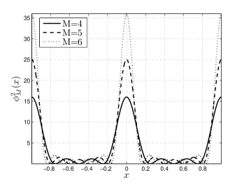
Figure 1: Square of ฯ•Mโ€‹(x)subscriptitalic-ฯ•๐‘€๐‘ฅ\phi_{M}\left(x\right) for different values of M๐‘€M.

We also need the trace of ๐Œ2superscript๐Œ2\mathbf{M}^{2}. Since ๐Œ๐Œ\mathbf{M} is a Hermitian matrix, it is true that

trโ€‹(๐Œ2)trsuperscript๐Œ2\displaystyle\mathrm{tr}\left(\mathbf{M}^{2}\right) =โˆ‘k1=0Kโˆ’1โˆ‘k2=0Kโˆ’1|ฮดk1,k2|2absentsuperscriptsubscriptsubscript๐‘˜10๐พ1superscriptsubscriptsubscript๐‘˜20๐พ1superscriptsubscript๐›ฟsubscript๐‘˜1subscript๐‘˜22\displaystyle=\sum_{k_{1}=0}^{K-1}\sum_{k_{2}=0}^{K-1}\left|\delta_{k_{1},k_{2}}\right|^{2}
โ‰กโˆ‘k1=0Kโˆ’1{Mt2+โˆ‘k2=0k1โ‰ k2Kโˆ’1|โˆ‘m=0Mtโˆ’1ejโ€‹2โ€‹ฯ€โ€‹mโ€‹(ฮฑk1tโˆ’ฮฑk2t)|2}absentsuperscriptsubscriptsubscript๐‘˜10๐พ1superscriptsubscript๐‘€๐‘ก2superscriptsubscriptsubscript๐‘˜20subscript๐‘˜1subscript๐‘˜2๐พ1superscriptsuperscriptsubscript๐‘š0subscript๐‘€๐‘ก1superscript๐‘’๐‘—2๐œ‹๐‘šsuperscriptsubscript๐›ผsubscript๐‘˜1๐‘กsuperscriptsubscript๐›ผsubscript๐‘˜2๐‘ก2\displaystyle\equiv\sum_{k_{1}=0}^{K-1}\left\{M_{t}^{2}+\sum_{\begin{subarray}{c}k_{2}=0\\ k_{1}\neq k_{2}\end{subarray}}^{K-1}\left|{\displaystyle\sum_{m=0}^{M_{t}-1}}e^{j2\pi m\left(\alpha_{k_{1}}^{t}-\alpha_{k_{2}}^{t}\right)}\right|^{2}\right\}
=โˆ‘k1=0Kโˆ’1{Mt2+โˆ‘k2=0k1โ‰ k2Kโˆ’1sin2โก(ฯ€โ€‹Mtโ€‹(ฮฑk1tโˆ’ฮฑk2t))sin2โก(ฯ€โ€‹(ฮฑk1tโˆ’ฮฑk2t))}absentsuperscriptsubscriptsubscript๐‘˜10๐พ1superscriptsubscript๐‘€๐‘ก2superscriptsubscriptsubscript๐‘˜20subscript๐‘˜1subscript๐‘˜2๐พ1superscript2๐œ‹subscript๐‘€๐‘กsuperscriptsubscript๐›ผsubscript๐‘˜1๐‘กsuperscriptsubscript๐›ผsubscript๐‘˜2๐‘กsuperscript2๐œ‹superscriptsubscript๐›ผsubscript๐‘˜1๐‘กsuperscriptsubscript๐›ผsubscript๐‘˜2๐‘ก\displaystyle=\sum_{k_{1}=0}^{K-1}\left\{M_{t}^{2}+\sum_{\begin{subarray}{c}k_{2}=0\\ k_{1}\neq k_{2}\end{subarray}}^{K-1}\dfrac{\sin^{2}\left(\pi M_{t}\left(\alpha_{k_{1}}^{t}-\alpha_{k_{2}}^{t}\right)\right)}{\sin^{2}\left(\pi\left(\alpha_{k_{1}}^{t}-\alpha_{k_{2}}^{t}\right)\right)}\right\}
โ‰œโˆ‘k1=0Kโˆ’1{Mt2+โˆ‘k2=0k1โ‰ k2Kโˆ’1ฯ•Mt2โ€‹(ฮฑk1tโˆ’ฮฑk2t)}.โ‰œabsentsuperscriptsubscriptsubscript๐‘˜10๐พ1superscriptsubscript๐‘€๐‘ก2superscriptsubscriptsubscript๐‘˜20subscript๐‘˜1subscript๐‘˜2๐พ1superscriptsubscriptitalic-ฯ•subscript๐‘€๐‘ก2superscriptsubscript๐›ผsubscript๐‘˜1๐‘กsuperscriptsubscript๐›ผsubscript๐‘˜2๐‘ก\displaystyle\triangleq\sum_{k_{1}=0}^{K-1}\left\{M_{t}^{2}+\sum_{\begin{subarray}{c}k_{2}=0\\ k_{1}\neq k_{2}\end{subarray}}^{K-1}\phi_{M_{t}}^{2}\left(\alpha_{k_{1}}^{t}-\alpha_{k_{2}}^{t}\right)\right\}. (46)

At this point, it is instructive to at least qualitatively study the behavior of the square of ฯ•Mโ€‹(x)subscriptitalic-ฯ•๐‘€๐‘ฅ\phi_{M}\left(x\right) (for a general parameter Mโˆˆโ„•+๐‘€superscriptโ„•M\in\mathbb{N}^{+}) defined above111This function constitutes a trivial variation of the so called Dirichlet kernel or periodic sinc function.. Fig. 1 shows the square of the function for three different values of M๐‘€M. We can directly identify the following useful fact:

Fact 1.

If

xโˆˆ[k,k+12],โˆ€kโˆˆโ„ค,formulae-sequence๐‘ฅ๐‘˜๐‘˜12for-all๐‘˜โ„คx\in\left[k,k+\dfrac{1}{2}\right],\>\forall\,k\in\mathbb{Z}, (47)

then the entire sequence of local maxima of ฯ•M2โ€‹(x)superscriptsubscriptitalic-ฯ•๐‘€2๐‘ฅ\phi_{M}^{2}\left(x\right) is strictly decreasing.

Next, define the function g:โ„+โ†’โ„+:๐‘”โ†’subscriptโ„subscriptโ„g:\mathbb{R}_{+}\rightarrow\mathbb{R}_{+} as

gโ€‹(x)โ‰œ{โŒˆxโŒ‰โˆ’x,โŒˆxโŒ‰โˆ’xโ‰ค12xโˆ’โŒŠxโŒ‹,otherwiseโ‰œ๐‘”๐‘ฅcases๐‘ฅ๐‘ฅ๐‘ฅ๐‘ฅ12๐‘ฅ๐‘ฅotherwiseg\left(x\right)\triangleq\begin{cases}\left\lceil x\right\rceil-x,&\left\lceil x\right\rceil-x\leq\dfrac{1}{2}\\ x-\left\lfloor x\right\rfloor,&\text{otherwise}\end{cases} (48)

and let

ฮพtโ‰œmin(i,j)โˆˆโ„•Kโˆ’1ร—โ„•Kโˆ’1iโ‰ jโกgโ€‹(|ฮฑitโˆ’ฮฑjt|)โˆˆ[0,12].โ‰œsubscript๐œ‰๐‘กsubscript๐‘–๐‘—subscriptโ„•๐พ1subscriptโ„•๐พ1๐‘–๐‘—๐‘”superscriptsubscript๐›ผ๐‘–๐‘กsuperscriptsubscript๐›ผ๐‘—๐‘ก012\xi_{t}\triangleq\min_{\begin{subarray}{c}\left(i,j\right)\in\mathbb{N}_{K-1}\times\mathbb{N}_{K-1}\\ i\neq j\end{subarray}}g\left(\left|\alpha_{i}^{t}-\alpha_{j}^{t}\right|\right)\in\left[0,\dfrac{1}{2}\right]. (49)

The motivation for defining ฮพtsubscript๐œ‰๐‘ก\xi_{t} stems from the fact that the function ฯ•M2โ€‹(x)superscriptsubscriptitalic-ฯ•๐‘€2๐‘ฅ\phi_{M}^{2}\left(x\right) is both periodic with unitary period and symmetric and thus it suffices to study its behavior only for xโˆˆ[0,12]๐‘ฅ012x\in\left[0,\dfrac{1}{2}\right]. Then, due to Fact 1, we can upper bound (46) as

trโ€‹(๐Œ2)trsuperscript๐Œ2\displaystyle\mathrm{tr}\left(\mathbf{M}^{2}\right) โ‰คโˆ‘k1=0Kโˆ’1{Mt2+(Kโˆ’1)โ€‹supxโˆˆ[ฮพt,12]ฯ•Mt2โ€‹(x)}absentsuperscriptsubscriptsubscript๐‘˜10๐พ1superscriptsubscript๐‘€๐‘ก2๐พ1subscriptsupremum๐‘ฅsubscript๐œ‰๐‘ก12superscriptsubscriptitalic-ฯ•subscript๐‘€๐‘ก2๐‘ฅ\displaystyle\leq\sum_{k_{1}=0}^{K-1}\left\{M_{t}^{2}+\left(K-1\right)\sup_{x\in\left[\xi_{t},\frac{1}{2}\right]}\phi_{M_{t}}^{2}\left(x\right)\right\} (50)
โ‰œKโ€‹Mt2+Kโ€‹(Kโˆ’1)โ€‹ฮฒฮพtโ€‹(Mt).โ‰œabsent๐พsuperscriptsubscript๐‘€๐‘ก2๐พ๐พ1subscript๐›ฝsubscript๐œ‰๐‘กsubscript๐‘€๐‘ก\displaystyle\triangleq KM_{t}^{2}+K\left(K-1\right)\beta_{\xi_{t}}\left(M_{t}\right). (51)

Consequently, by Theorem 4,

s2superscript๐‘ 2\displaystyle s^{2} =trโ€‹(๐Œ2)Kโˆ’Mt2absenttrsuperscript๐Œ2๐พsuperscriptsubscript๐‘€๐‘ก2\displaystyle=\dfrac{\mathrm{tr}\left(\mathbf{M}^{2}\right)}{K}-M_{t}^{2}
โ‰คMt2+ฮฒฮพโ€‹(Mt)โ€‹(Kโˆ’1)โˆ’Mt2absentsuperscriptsubscript๐‘€๐‘ก2subscript๐›ฝ๐œ‰subscript๐‘€๐‘ก๐พ1superscriptsubscript๐‘€๐‘ก2\displaystyle\leq M_{t}^{2}+\beta_{\xi}\left(M_{t}\right)\left(K-1\right)-M_{t}^{2}
โ‰กฮฒฮพtโ€‹(Mt)โ€‹(Kโˆ’1)absentsubscript๐›ฝsubscript๐œ‰๐‘กsubscript๐‘€๐‘ก๐พ1\displaystyle\equiv\beta_{\xi_{t}}\left(M_{t}\right)\left(K-1\right) (52)

and consequently we can bound ฮปmโ€‹iโ€‹nโ€‹(๐Œ)โ‰กฮปmโ€‹iโ€‹nโ€‹(๐—t๐‘ฏโ€‹๐—t)subscript๐œ†๐‘š๐‘–๐‘›๐Œsubscript๐œ†๐‘š๐‘–๐‘›superscriptsubscript๐—๐‘ก๐‘ฏsubscript๐—๐‘ก\lambda_{min}\left(\mathbf{M}\right)\equiv\lambda_{min}\left(\mathbf{X}_{t}^{\boldsymbol{\mathit{H}}}\mathbf{X}_{t}\right) from below as

ฮปmโ€‹iโ€‹nโ€‹(๐—t๐‘ฏโ€‹๐—t)โ‰ฅMtโˆ’(Kโˆ’1)โ€‹ฮฒฮพtโ€‹(Mt).subscript๐œ†๐‘š๐‘–๐‘›superscriptsubscript๐—๐‘ก๐‘ฏsubscript๐—๐‘กsubscript๐‘€๐‘ก๐พ1subscript๐›ฝsubscript๐œ‰๐‘กsubscript๐‘€๐‘ก\lambda_{min}\left(\mathbf{X}_{t}^{\boldsymbol{\mathit{H}}}\mathbf{X}_{t}\right)\geq M_{t}-\left(K-1\right)\sqrt{\beta_{\xi_{t}}\left(M_{t}\right)}. (53)

Respectively, we get

ฮปmโ€‹iโ€‹nโ€‹(๐—r๐‘ฏโ€‹๐—r)โ‰ฅMrโˆ’(Kโˆ’1)โ€‹ฮฒฮพrโ€‹(Mr).subscript๐œ†๐‘š๐‘–๐‘›superscriptsubscript๐—๐‘Ÿ๐‘ฏsubscript๐—๐‘Ÿsubscript๐‘€๐‘Ÿ๐พ1subscript๐›ฝsubscript๐œ‰๐‘Ÿsubscript๐‘€๐‘Ÿ\lambda_{min}\left(\mathbf{X}_{r}^{\boldsymbol{\mathit{H}}}\mathbf{X}_{r}\right)\geq M_{r}-\left(K-1\right)\sqrt{\beta_{\xi_{r}}\left(M_{r}\right)}. (54)

Therefore, for fixed Mtsubscript๐‘€๐‘กM_{t} and Mrsubscript๐‘€๐‘ŸM_{r}, as long as

Kโ‰คmaxiโˆˆ{t,r}โก{Miฮฒฮพiโ€‹(Mi)},๐พsubscript๐‘–๐‘ก๐‘Ÿsubscript๐‘€๐‘–subscript๐›ฝsubscript๐œ‰๐‘–subscript๐‘€๐‘–K\leq\max_{i\in\left\{t,r\right\}}\left\{\dfrac{M_{i}}{\sqrt{\beta_{\xi_{i}}\left(M_{i}\right)}}\right\}, (55)

the upper bounds

ฮผโ€‹(U)๐œ‡๐‘ˆ\displaystyle\mu\left(U\right) โ‰คMtMtโˆ’(Kโˆ’1)โ€‹ฮฒฮพtโ€‹(Mt)andabsentsubscript๐‘€๐‘กsubscript๐‘€๐‘ก๐พ1subscript๐›ฝsubscript๐œ‰๐‘กsubscript๐‘€๐‘กand\displaystyle\leq\dfrac{M_{t}}{M_{t}-\left(K-1\right)\sqrt{\beta_{\xi_{t}}\left(M_{t}\right)}}\quad\text{and} (56)
ฮผโ€‹(V)๐œ‡๐‘‰\displaystyle\mu\left(V\right) โ‰คMrMrโˆ’(Kโˆ’1)โ€‹ฮฒฮพrโ€‹(Mr)absentsubscript๐‘€๐‘Ÿsubscript๐‘€๐‘Ÿ๐พ1subscript๐›ฝsubscript๐œ‰๐‘Ÿsubscript๐‘€๐‘Ÿ\displaystyle\leq\dfrac{M_{r}}{M_{r}-\left(K-1\right)\sqrt{\beta_{\xi_{r}}\left(M_{r}\right)}} (57)

both hold true with probability 1. Consequently,

maxโก{ฮผโ€‹(U),ฮผโ€‹(V)}โ‰คmaxiโˆˆ{t,r}โก{MiMiโˆ’(Kโˆ’1)โ€‹ฮฒฮพiโ€‹(Mi)}โ‰œฮผ0.๐œ‡๐‘ˆ๐œ‡๐‘‰subscript๐‘–๐‘ก๐‘Ÿsubscript๐‘€๐‘–subscript๐‘€๐‘–๐พ1subscript๐›ฝsubscript๐œ‰๐‘–subscript๐‘€๐‘–โ‰œsubscript๐œ‡0\max\left\{\mu\left(U\right),\mu\left(V\right)\right\}\leq\max_{i\in\left\{t,r\right\}}\left\{\dfrac{M_{i}}{M_{i}-\left(K-1\right)\sqrt{\beta_{\xi_{i}}\left(M_{i}\right)}}\right\}\triangleq\mu_{0}. (58)

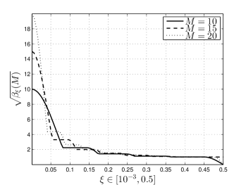
Fig. 2 depicts the parameter ฮฒฮพโ€‹(M)subscript๐›ฝ๐œ‰๐‘€\sqrt{\beta_{\xi}\left(M\right)} (either for ฮพrsubscript๐œ‰๐‘Ÿ\xi_{r} or ฮพtsubscript๐œ‰๐‘ก\xi_{t} and Mrsubscript๐‘€๐‘ŸM_{r} or Mtsubscript๐‘€๐‘กM_{t}) as a function of ฮพ๐œ‰\xi for three values of M๐‘€M.

Refer to caption
Figure 2: Values of ฮฒฮพโ€‹(M)subscript๐›ฝ๐œ‰๐‘€\sqrt{\beta_{\xi}\left(M\right)} for different values of M๐‘€M.

Further, the following fact also holds true, stemming directly from the behavior of ฯ•M2โ€‹(x)superscriptsubscriptitalic-ฯ•๐‘€2๐‘ฅ\phi_{M}^{2}\left(x\right) (also see Fig. 1).

Refer to caption
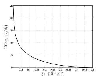
Figure 3: Values of ฮฒฮพsubscript๐›ฝ๐œ‰\sqrt{\beta_{\xi}} in the interval [10โˆ’3,0.5]superscript1030.5\left[10^{-3},0.5\right].
Fact 2.

Restricting our attention at the principal period of ฯ•M2โ€‹(x)superscriptsubscriptitalic-ฯ•๐‘€2๐‘ฅ\phi_{M}^{2}\left(x\right) ([โˆ’1,1]11\left[-1,1\right]), as M is getting larger, the main lobe of the function gets taller and narrower. Also, by definition of ฯ•M2โ€‹(x)superscriptsubscriptitalic-ฯ•๐‘€2๐‘ฅ\phi_{M}^{2}\left(x\right), it follows that for any Mโˆˆโ„•+๐‘€superscriptโ„•M\in\mathbb{N}^{+} (and even when Mโ†’โˆžโ†’๐‘€M\rightarrow\infty), the function possesses only one singularity (in the principal period) occurring at xโ‰ก0๐‘ฅ0x\equiv 0.

Now, assume that ฮพโ‰œminโก{ฮพr,ฮพt}โ‰ 0โ‰œ๐œ‰subscript๐œ‰๐‘Ÿsubscript๐œ‰๐‘ก0\xi\triangleq\min\left\{\xi_{r},\xi_{t}\right\}\neq 0. Then, we can write

ฮฒฮพtโ€‹(Mt)subscript๐›ฝsubscript๐œ‰๐‘กsubscript๐‘€๐‘ก\displaystyle\beta_{\xi_{t}}\left(M_{t}\right) โ‰กsupxโˆˆ[ฮพt,12]ฯ•Mt2โ€‹(x)absentsubscriptsupremum๐‘ฅsubscript๐œ‰๐‘ก12superscriptsubscriptitalic-ฯ•subscript๐‘€๐‘ก2๐‘ฅ\displaystyle\equiv\sup_{x\in\left[\xi_{t},\frac{1}{2}\right]}\phi_{M_{t}}^{2}\left(x\right)
โ‰คsupxโˆˆ[ฮพ,12]ฯ•Mt2โ€‹(x)absentsubscriptsupremum๐‘ฅ๐œ‰12superscriptsubscriptitalic-ฯ•subscript๐‘€๐‘ก2๐‘ฅ\displaystyle\leq\sup_{x\in\left[\xi,\frac{1}{2}\right]}\phi_{M_{t}}^{2}\left(x\right)
โ‰คsupxโˆˆ[ฮพ,12]Mtโˆˆโ„•+ฯ•Mt2โ€‹(x)โ‰กsupxโˆˆ[ฮพ,12]Mrโˆˆโ„•+ฯ•Mr2โ€‹(x)โ‰œฮฒฮพ.absentsubscriptsupremum๐‘ฅ๐œ‰12subscript๐‘€๐‘กsuperscriptโ„•superscriptsubscriptitalic-ฯ•subscript๐‘€๐‘ก2๐‘ฅsubscriptsupremum๐‘ฅ๐œ‰12subscript๐‘€๐‘Ÿsuperscriptโ„•superscriptsubscriptitalic-ฯ•subscript๐‘€๐‘Ÿ2๐‘ฅโ‰œsubscript๐›ฝ๐œ‰\displaystyle\leq\sup_{\begin{subarray}{c}x\in\left[\xi,\frac{1}{2}\right]\\ M_{t}\in\mathbb{N}^{+}\end{subarray}}\phi_{M_{t}}^{2}\left(x\right)\equiv\sup_{\begin{subarray}{c}x\in\left[\xi,\frac{1}{2}\right]\\ M_{r}\in\mathbb{N}^{+}\end{subarray}}\phi_{M_{r}}^{2}\left(x\right)\triangleq\beta_{\xi}. (59)

Since ฮพโ‰ 0๐œ‰0\xi\neq 0 by assumption and due to Fact 2, the supremum appearing in (59) will be always finite and, consequently the respective bound will be non trivial.

Therefore, in this case, for fixed K๐พK, (55) becomes

miniโˆˆ{t,r}โกMiโ‰ฅKโ€‹ฮฒฮพ=๐’ชโ€‹(K).subscript๐‘–๐‘ก๐‘Ÿsubscript๐‘€๐‘–๐พsubscript๐›ฝ๐œ‰๐’ช๐พ\min_{i\in\left\{t,r\right\}}M_{i}\geq K\sqrt{\beta_{\xi}}=\mathcal{O}\left(K\right). (60)

Passing to the limit with respect to Mtsubscript๐‘€๐‘กM_{t} (respectively Mrsubscript๐‘€๐‘ŸM_{r}), we get

lim supMtโ†’โˆžฮผโ€‹(U)subscriptlimit-supremumโ†’subscript๐‘€๐‘ก๐œ‡๐‘ˆ\displaystyle\limsup_{M_{t}\rightarrow\infty}\mu\left(U\right) โ‰คlim supMtโ†’โˆžMtMtโˆ’(Kโˆ’1)โ€‹ฮฒฮพabsentsubscriptlimit-supremumโ†’subscript๐‘€๐‘กsubscript๐‘€๐‘กsubscript๐‘€๐‘ก๐พ1subscript๐›ฝ๐œ‰\displaystyle\leq\limsup_{M_{t}\rightarrow\infty}\dfrac{M_{t}}{M_{t}-\left(K-1\right)\sqrt{\beta_{\xi}}}
โ‰กlimMtโ†’โˆžMtMtโˆ’(Kโˆ’1)โ€‹ฮฒฮพ=1absentsubscriptโ†’subscript๐‘€๐‘กsubscript๐‘€๐‘กsubscript๐‘€๐‘ก๐พ1subscript๐›ฝ๐œ‰1\displaystyle\equiv\lim_{M_{t}\rightarrow\infty}\dfrac{M_{t}}{M_{t}-\left(K-1\right)\sqrt{\beta_{\xi}}}=1 (61)

and since ฮผโ€‹(U)โ‰ฅ1๐œ‡๐‘ˆ1\mu\left(U\right)\geq 1 by definition [4], it must be true that, in the limit, ฮผโ€‹(U)โ‰ก1๐œ‡๐‘ˆ1\mu\left(U\right)\equiv 1. Likewise, it will also be true that, in the limit, ฮผโ€‹(V)โ‰ก1๐œ‡๐‘‰1\mu\left(V\right)\equiv 1.

If additionally ฮพ๐œ‰\xi is safely bounded away from zero, then ฮฒฮพsubscript๐›ฝ๐œ‰\beta_{\xi} will be small (due to Fact 1) and thus for sufficiently large but finite Mtsubscript๐‘€๐‘กM_{t} and Mrsubscript๐‘€๐‘ŸM_{r},

ฮผโ€‹(U)โ‰ˆฮผโ€‹(V)โ‰ˆ1.๐œ‡๐‘ˆ๐œ‡๐‘‰1\mu\left(U\right)\approx\mu\left(V\right)\approx 1. (62)

An experimental calculation of the square root of the supremum ฮฒฮพsubscript๐›ฝ๐œ‰\beta_{\xi} for ฮพโˆˆ[10โˆ’3,0.5]๐œ‰superscript1030.5\xi\in\left[10^{-3},0.5\right] shown in Fig. 3 (in logarithmic scale) can validate and possibly strengthen our theoretical arguments presented above. We observe that ฮฒฮพsubscript๐›ฝ๐œ‰\sqrt{\beta_{\xi}} over ฮพ๐œ‰\xi constitutes a hyperbolic function, converging rapidly to 1 (linear scale), which corresponds to its minimum value.

Finally, regarding the Assumption ๐€๐Ÿ๐€๐Ÿ\mathbf{A1}, by a simple argument involving the Cauchy - Schwarz inequality, it can be shown that [4], in the general case, one can choose

ฮผ1โ‰œฮผ0โ€‹K=maxiโˆˆ{t,r}โก{Miโ€‹KMiโˆ’(Kโˆ’1)โ€‹ฮฒฮพiโ€‹(Mi)},โ‰œsubscript๐œ‡1subscript๐œ‡0๐พsubscript๐‘–๐‘ก๐‘Ÿsubscript๐‘€๐‘–๐พsubscript๐‘€๐‘–๐พ1subscript๐›ฝsubscript๐œ‰๐‘–subscript๐‘€๐‘–\mu_{1}\triangleq\mu_{0}\sqrt{K}=\max_{i\in\left\{t,r\right\}}\left\{\dfrac{M_{i}\sqrt{K}}{M_{i}-\left(K-1\right)\sqrt{\beta_{\xi_{i}}\left(M_{i}\right)}}\right\}, (63)

holding true also with probability 1. The results presented in the statement of Theorem 3 readily follow.โˆŽ

In colocated MIMO Radar systems, due to the need for unambiguous angle estimation (target detection), it is very common to assume that ฮธiโˆˆ[โˆ’ฯ€/2,ฯ€/2],โˆ€iโˆˆโ„•Kโˆ’1formulae-sequencesubscript๐œƒ๐‘–๐œ‹2๐œ‹2for-all๐‘–subscriptโ„•๐พ1\theta_{i}\in\left[-\pi/2,\pi/2\right],\forall\,i\in\mathbb{N}_{K-1}. Also, especially for the case where ULAs are employed for transmission and reception, another common assumption is to choose drโ‰กdt=ฮป/2subscript๐‘‘๐‘Ÿsubscript๐‘‘๐‘ก๐œ†2d_{r}\equiv d_{t}=\lambda/2. Under this setting, the following lemma provides a simple sufficient condition, which guarantees that the asymptotics of Theorem 3 hold true and, as a result, that for a sufficiently large number of transmission/reception antennas, the coherence of ๐šซ๐šซ\boldsymbol{\Delta} will be small.

Lemma 2.

(ULA Pairs Coherence Control) Consider the hypotheses and definitions of Theorem 3. Set drโ‰กdt=ฮป/2subscript๐‘‘๐‘Ÿsubscript๐‘‘๐‘ก๐œ†2d_{r}\equiv d_{t}=\lambda/2. If additionally

(ฮธi,ฮธj)โˆˆ๐’œ,withsubscript๐œƒ๐‘–subscript๐œƒ๐‘—๐’œwith\displaystyle\left(\theta_{i},\theta_{j}\right)\in\mathcal{A},\quad\text{with} (64)
๐’œโ‰œ{(x,y)โˆˆ[โˆ’ฯ€2,ฯ€2]2|ฮทโ‰ค|yโˆ’x|โ‰คฯ€โˆ’ฮท}โ‰œ๐’œconditional-set๐‘ฅ๐‘ฆsuperscript๐œ‹2๐œ‹22๐œ‚๐‘ฆ๐‘ฅ๐œ‹๐œ‚\displaystyle\mathcal{A}\triangleq\left\{\left.\left(x,y\right)\in\left[-\dfrac{\pi}{2},\dfrac{\pi}{2}\right]^{2}\right|\eta\leq\left|y-x\right|\leq\pi-\eta\right\} (65)

โˆ€(i,j)โˆˆโ„•Kโˆ’1ร—โ„•Kโˆ’1for-all๐‘–๐‘—subscriptโ„•๐พ1subscriptโ„•๐พ1\forall\,\left(i,j\right)\in\mathbb{N}_{K-1}\times\mathbb{N}_{K-1} with iโ‰ j๐‘–๐‘—i\neq j and for some apriori chosen ฮทโˆˆ(0,ฯ€2]๐œ‚0๐œ‹2\eta\in\left(0,\dfrac{\pi}{2}\right], then

ฮพ=1โˆ’cosโก(ฮท2)โˆˆ(0,2โˆ’22]๐œ‰1๐œ‚20222\xi=1-\cos\left(\dfrac{\eta}{2}\right)\in\left(0,\dfrac{2-\sqrt{2}}{2}\right] (66)

and the asymptotics of Theorem 3 always hold true. In particular, the higher the value of ฮท๐œ‚\eta, the higher the value of ฮพ๐œ‰\xi and the lower the coherence of ๐šซ๐šซ\boldsymbol{\Delta}.

Proof of Lemma 2.

See Appendix B.โˆŽ

III-B Near Optimal Recoverability of ๐šซ๐šซ\boldsymbol{\Delta}

Using Lemma 1, we can now directly combine Theorem 2 with the coherence results presented in the previous subsection, producing (asymptotic) bounds regarding the number of observations required for the exact reconstruction of the matrix ๐šซ๐šซ\boldsymbol{\Delta} by solving the convex program (1). Specifically for ULA transmitter/receiver pairs, we present the following interesting result. Since the proof is straightforward, it is omitted.

Theorem 5.

(Near Optimal Recoverability for ULA Pairs) Consider the hypotheses of Theorem 3 and assume that ฮพ๐œ‰\xi is safely bounded away from zero. Also, set Mโ‰œmaxโก{Mr,Mt}โ‰œ๐‘€subscript๐‘€๐‘Ÿsubscript๐‘€๐‘กM\triangleq\max\left\{M_{r},M_{t}\right\}. Suppose we observe m๐‘šm entries of ๐šซ๐šซ\boldsymbol{\Delta} with locations sampled uniformly at random. Then, for Mrsubscript๐‘€๐‘ŸM_{r} and Mtsubscript๐‘€๐‘กM_{t} sufficiently large satisfying

miniโˆˆ{t,r}โกMiโ‰ฅKโ€‹ฮฒฮพsubscript๐‘–๐‘ก๐‘Ÿsubscript๐‘€๐‘–๐พsubscript๐›ฝ๐œ‰\min_{i\in\left\{t,r\right\}}M_{i}\geq K\sqrt{\beta_{\xi}} (67)

for a fixed number of targets K๐พK, ๐šซ๐šซ\boldsymbol{\Delta} is strongly incoherent with parameter

ฮผโ‰คฮผ0โ€‹Kโ‰ˆK๐œ‡subscript๐œ‡0๐พ๐พ\mu\leq\mu_{0}\sqrt{K}\approx\sqrt{K} (68)

and there exist positive numerical constants C1subscript๐ถ1C_{1} and C2subscript๐ถ2C_{2} such that if

m๐‘š\displaystyle m โ‰ณC1โ€‹K4โ€‹Mโ€‹log2โกM=๐’ชโ€‹(Mโ€‹log2โกM)orformulae-sequencegreater-than-or-equivalent-toabsentsubscript๐ถ1superscript๐พ4๐‘€superscript2๐‘€๐’ช๐‘€superscript2๐‘€or\displaystyle\gtrsim C_{1}K^{4}M\log^{2}M=\mathcal{O}\left(M\log^{2}M\right)\quad\text{or} (69)
m๐‘š\displaystyle m โ‰ณC2โ€‹K2โ€‹Mโ€‹log6โกM=๐’ชโ€‹(Mโ€‹log6โกM),greater-than-or-equivalent-toabsentsubscript๐ถ2superscript๐พ2๐‘€superscript6๐‘€๐’ช๐‘€superscript6๐‘€\displaystyle\gtrsim C_{2}K^{2}M\log^{6}M=\mathcal{O}\left(M\log^{6}M\right), (70)

the minimizer to the program (1) is unique and equal to ๐šซ๐šซ\boldsymbol{\Delta} with probability at least 1โˆ’Mโˆ’31superscript๐‘€31-M^{-3}.

Roughly speaking, Theorem 5 implies that as long as ULAs are concerned, for a sufficiently large number of transmission and reception antennas and for a fixed and relatively small number of targets, matrix completion is exact if the number of observations is at least of an order of Mโ€‹polylogโ€‹(M)๐‘€polylog๐‘€M\mathrm{polylog}\left(M\right), that is, matrix completion is exact for a slightly larger number of observations than the information theoretic limit (see [5] for details).

IV Coherence of ๐šซ๐šซ\boldsymbol{\Delta} for Arbitrary 2D Arrays

It is possible to generalize Theorem 3 for a far more general case, that is, when the transmitter and the receiver employ arbitrary 222-dimensional arrays. However, in this case, since our knowledge about the specific characteristics of the topologies of the arrays involved is very restricted, our bounds, although tight, are not expected to be as easily handleable as in the ULA case (see Theorem 3 and Lemma 2). Next, we state and prove the following theorem in this respect.

Theorem 6.

(Coherence for Arbitrary 2D Arrays) Consider an arbitrary array transmitter - receiver pair equipped with Mtsubscript๐‘€๐‘กM_{t} and Mrsubscript๐‘€๐‘ŸM_{r} antennas, respectively. Assume that the set of target angles {ฮธk}kโˆˆโ„•Kโˆ’1subscriptsubscript๐œƒ๐‘˜๐‘˜subscriptโ„•๐พ1\left\{\theta_{k}\right\}_{k\in\mathbb{N}_{K-1}} consists of almost surely distinct members and that

(ฮธi,ฮธj)โˆˆ๐’œโŠ†โ„2โˆ’{(x,y)โˆˆโ„2|xโ‰ y}subscript๐œƒ๐‘–subscript๐œƒ๐‘—๐’œsuperscriptโ„2conditional-set๐‘ฅ๐‘ฆsuperscriptโ„2๐‘ฅ๐‘ฆ\left(\theta_{i},\theta_{j}\right)\in\mathcal{A}\subseteq\mathbb{R}^{2}-\left\{\left.\left(x,y\right)\in\mathbb{R}^{2}\right|x\neq y\right\} (71)

โˆ€(i,j)โˆˆโ„•Kโˆ’1ร—โ„•Kโˆ’1for-all๐‘–๐‘—subscriptโ„•๐พ1subscriptโ„•๐พ1\forall\,\left(i,j\right)\in\mathbb{N}_{K-1}\times\mathbb{N}_{K-1} with iโ‰ j๐‘–๐‘—i\neq j, where ๐’œ๐’œ\mathcal{A} constitutes a nominal point set for all admissible angle pair combinations. Also, let the abstract sets ๐”—๐”—\mathfrak{T} and โ„œโ„œ\mathfrak{R} contain all the essential information regarding the transmitter and receiver topologies, also assumed fixed and known apriori. Then, for any Mtsubscript๐‘€๐‘กM_{t} and Mrsubscript๐‘€๐‘ŸM_{r}, as long as

Kโ‰คmaxiโˆˆ{t,r}โก{Miฮฒi},๐พsubscript๐‘–๐‘ก๐‘Ÿsubscript๐‘€๐‘–subscript๐›ฝ๐‘–K\leq\max_{i\in\left\{t,r\right\}}\left\{\dfrac{M_{i}}{\sqrt{\beta_{i}}}\right\}, (72)

the associated matrix ๐šซ๐šซ\boldsymbol{\Delta} obeys the assumptions ๐€๐ŸŽ๐€๐ŸŽ\mathbf{A0} and ๐€๐Ÿ๐€๐Ÿ\mathbf{A1} with

ฮผ0subscript๐œ‡0\displaystyle\mu_{0} โ‰œmaxiโˆˆ{t,r}โก{MiMiโˆ’(Kโˆ’1)โ€‹ฮฒi}andโ‰œabsentsubscript๐‘–๐‘ก๐‘Ÿsubscript๐‘€๐‘–subscript๐‘€๐‘–๐พ1subscript๐›ฝ๐‘–and\displaystyle\triangleq\max_{i\in\left\{t,r\right\}}\left\{\dfrac{M_{i}}{M_{i}-\left(K-1\right)\sqrt{\beta_{i}}}\right\}\quad\text{and} (73)
ฮผ1subscript๐œ‡1\displaystyle\mu_{1} โ‰œmaxiโˆˆ{t,r}โก{Miโ€‹KMiโˆ’(Kโˆ’1)โ€‹ฮฒi}โ‰œabsentsubscript๐‘–๐‘ก๐‘Ÿsubscript๐‘€๐‘–๐พsubscript๐‘€๐‘–๐พ1subscript๐›ฝ๐‘–\displaystyle\triangleq\max_{i\in\left\{t,r\right\}}\left\{\dfrac{M_{i}\sqrt{K}}{M_{i}-\left(K-1\right)\sqrt{\beta_{i}}}\right\} (74)

with probability 111 and where

ฮฒtโ€‹(r)subscript๐›ฝ๐‘ก๐‘Ÿ\displaystyle\beta_{t\left(r\right)} โ‰œsup(x,y)โˆˆ๐’œ|ฯ†tโ€‹(r)(x,y|๐”—(โ„œ))|2โˆˆ[0,Mtโ€‹(r)2),\displaystyle\triangleq\sup_{\left(x,y\right)\in\mathcal{A}}\left|\varphi_{t\left(r\right)}\left(x,y\left|\mathfrak{T}\left(\mathfrak{R}\right)\right.\right)\right|^{2}\in\left[0,M_{t\left(r\right)}^{2}\right), (75)

with ฯ†tโ€‹(r):๐’œโ†’โ„‚:subscript๐œ‘๐‘ก๐‘Ÿโ†’๐’œโ„‚\varphi_{t\left(r\right)}:\mathcal{A}\rightarrow\mathbb{C} given by

ฯ†tโ€‹(r)โ€‹(x,y|๐”—โ€‹(โ„œ))โ‰œโˆ‘m=0Mtโ€‹(r)โˆ’1expโก(jโ€‹2โ€‹ฯ€โ€‹๐ซtโ€‹(r)๐‘ปโ€‹(m)โ€‹(๐’ฏโ€‹(x)โˆ’๐’ฏโ€‹(y))),โ‰œsubscript๐œ‘๐‘ก๐‘Ÿ๐‘ฅconditional๐‘ฆ๐”—โ„œsuperscriptsubscript๐‘š0subscript๐‘€๐‘ก๐‘Ÿ1๐‘—2๐œ‹superscriptsubscript๐ซ๐‘ก๐‘Ÿ๐‘ป๐‘š๐’ฏ๐‘ฅ๐’ฏ๐‘ฆ\varphi_{t\left(r\right)}\left(x,y\left|\mathfrak{T}\left(\mathfrak{R}\right)\right.\right)\triangleq{\displaystyle\sum_{m=0}^{M_{t\left(r\right)}-1}}\exp\left(j2\pi\mathbf{r}_{t\left(r\right)}^{\boldsymbol{T}}\left(m\right)\left(\mathcal{T}\left(x\right)-\mathcal{T}\left(y\right)\right)\right), (76)

where

๐ซtโ€‹(r)โ€‹(l)subscript๐ซ๐‘ก๐‘Ÿ๐‘™\displaystyle\mathbf{r}_{t\left(r\right)}\left(l\right) โ‰œ1ฮปโ€‹[xltโ€‹(r)โ€‹yltโ€‹(r)]๐‘ปโˆˆโ„2ร—1,lโˆˆโ„•Mtโ€‹(r)โˆ’1formulae-sequenceโ‰œabsent1๐œ†superscriptdelimited-[]superscriptsubscript๐‘ฅ๐‘™๐‘ก๐‘Ÿsuperscriptsubscript๐‘ฆ๐‘™๐‘ก๐‘Ÿ๐‘ปsuperscriptโ„21๐‘™subscriptโ„•subscript๐‘€๐‘ก๐‘Ÿ1\displaystyle\triangleq\dfrac{1}{\lambda}\left[x_{l}^{t\left(r\right)}\,y_{l}^{t\left(r\right)}\right]^{\boldsymbol{T}}\in\mathbb{R}^{2\times 1},l\in\mathbb{N}_{M_{t\left(r\right)}-1} (77)
๐’ฏโ€‹(x)๐’ฏ๐‘ฅ\displaystyle\mathcal{T}\left(x\right) โ‰œ[cosโก(x)sinโก(x)]โˆˆโ„2ร—1,โ‰œabsentmatrix๐‘ฅ๐‘ฅsuperscriptโ„21\displaystyle\triangleq\begin{bmatrix}\cos\left(x\right)\\ \sin\left(x\right)\end{bmatrix}\in\mathbb{R}^{2\times 1}, (78)

with the collection of vectors {[xltโ€‹(r)โ€‹yltโ€‹(r)]๐“}lโˆˆโ„•Mtโ€‹(r)โˆ’1subscriptsuperscriptdelimited-[]superscriptsubscript๐‘ฅ๐‘™๐‘ก๐‘Ÿsuperscriptsubscript๐‘ฆ๐‘™๐‘ก๐‘Ÿ๐“๐‘™subscriptโ„•subscript๐‘€๐‘ก๐‘Ÿ1\left\{\left[x_{l}^{t\left(r\right)}\,y_{l}^{t\left(r\right)}\right]^{\boldsymbol{T}}\right\}_{l\in\mathbb{N}_{M_{t\left(r\right)}-1}} denoting the 222-dimensional antenna coordinates of the respective array.

Proof of Theorem 6.

Again, we divide the proof into the following subsections, in similar fashion as in the proof of Theorem 3.

IV-1 Characterization of the SVD of ๐šซ๐šซ\boldsymbol{\Delta}

We now consider the almost surely rank-K๐พK matrix

๐šซ=๐—rโ€‹๐ƒ๐—t๐‘ปโˆˆโ„‚Mtร—Mr,๐šซsubscript๐—๐‘Ÿsuperscriptsubscript๐ƒ๐—๐‘ก๐‘ปsuperscriptโ„‚subscript๐‘€๐‘กsubscript๐‘€๐‘Ÿ\boldsymbol{\Delta}=\mathbf{X}_{r}\mathbf{D}\mathbf{X}_{t}^{\boldsymbol{T}}\in\mathbb{C}^{M_{t}\times M_{r}}, (79)

exactly as defined in Subsection C of Section II. Of course, since ๐šซ๐šซ\boldsymbol{\Delta} is assumed to be of rank-K๐พK almost surely, the members of the set of angles {ฮธk}kโˆˆโ„•Kโˆ’1subscriptsubscript๐œƒ๐‘˜๐‘˜subscriptโ„•๐พ1\left\{\theta_{k}\right\}_{k\in\mathbb{N}_{K-1}} are implicitly assumed to be almost surely distinct.

By almost identical reasoning as in the proof of Theorem 3, the coherences of the column and row spaces of ๐šซ๐šซ\boldsymbol{\Delta}, U๐‘ˆU and V๐‘‰V, can be upper bounded using (41) and (42), respectively.

IV-2 Bounding ฮปmโ€‹iโ€‹nโ€‹(๐—tโ€‹(r)๐‘ฏโ€‹๐—tโ€‹(r))subscript๐œ†๐‘š๐‘–๐‘›superscriptsubscript๐—๐‘ก๐‘Ÿ๐‘ฏsubscript๐—๐‘ก๐‘Ÿ\lambda_{min}\left(\mathbf{X}_{t\left(r\right)}^{\boldsymbol{\mathit{H}}}\mathbf{X}_{t\left(r\right)}\right)

We directly focus on the matrix ๐—t๐‘ฏโ€‹๐—tโˆˆโ„‚Kร—Ksuperscriptsubscript๐—๐‘ก๐‘ฏsubscript๐—๐‘กsuperscriptโ„‚๐พ๐พ\mathbf{X}_{t}^{\boldsymbol{\mathit{H}}}\mathbf{X}_{t}\in\mathbb{C}^{K\times K} defined as in (43), where this time, โˆ€(i,j)โˆˆโ„•Kโˆ’1ร—โ„•Kโˆ’1for-all๐‘–๐‘—subscriptโ„•๐พ1subscriptโ„•๐พ1\forall\,\left(i,j\right)\in\mathbb{N}_{K-1}\times\mathbb{N}_{K-1},

ฮดi,jโ‰œโˆ‘m=0Mtโˆ’1ejโ€‹2โ€‹ฯ€โ€‹๐ซt๐‘ปโ€‹(m)โ€‹(๐’ฏโ€‹(ฮธi)โˆ’๐’ฏโ€‹(ฮธj)),โ‰œsubscript๐›ฟ๐‘–๐‘—superscriptsubscript๐‘š0subscript๐‘€๐‘ก1superscript๐‘’๐‘—2๐œ‹superscriptsubscript๐ซ๐‘ก๐‘ป๐‘š๐’ฏsubscript๐œƒ๐‘–๐’ฏsubscript๐œƒ๐‘—\displaystyle\delta_{i,j}\triangleq{\displaystyle\sum_{m=0}^{M_{t}-1}}e^{j2\pi\mathbf{r}_{t}^{\boldsymbol{T}}\left(m\right)\left(\mathcal{T}\left(\theta_{i}\right)-\mathcal{T}\left(\theta_{j}\right)\right)}, (80)

with Mtโ‰กฮดi,i,โˆ€iโˆˆโ„•Kโˆ’1formulae-sequencesubscript๐‘€๐‘กsubscript๐›ฟ๐‘–๐‘–for-all๐‘–subscriptโ„•๐พ1M_{t}\equiv\delta_{i,i},\forall\,i\in\mathbb{N}_{K-1}.

Applying Theorem 3 to ๐Œโ‰œ๐—t๐‘ฏโ€‹๐—tโˆˆโ„‚Kร—Kโ‰œ๐Œsuperscriptsubscript๐—๐‘ก๐‘ฏsubscript๐—๐‘กsuperscriptโ„‚๐พ๐พ\mathbf{M}\triangleq\mathbf{X}_{t}^{\boldsymbol{\mathit{H}}}\mathbf{X}_{t}\in\mathbb{C}^{K\times K}, we get ฯ„โ‰กMt๐œsubscript๐‘€๐‘ก\tau\equiv M_{t} and, concerning the trace of ๐Œ2superscript๐Œ2\mathbf{M}^{2}, it is true that

trโ€‹(๐Œ2)trsuperscript๐Œ2\displaystyle\mathrm{tr}\left(\mathbf{M}^{2}\right) =โˆ‘k1=0Kโˆ’1โˆ‘k2=0Kโˆ’1|ฮดk1,k2|2absentsuperscriptsubscriptsubscript๐‘˜10๐พ1superscriptsubscriptsubscript๐‘˜20๐พ1superscriptsubscript๐›ฟsubscript๐‘˜1subscript๐‘˜22\displaystyle=\sum_{k_{1}=0}^{K-1}\sum_{k_{2}=0}^{K-1}\left|\delta_{k_{1},k_{2}}\right|^{2}
=โˆ‘k1=0Kโˆ’1{Mt2+โˆ‘k2=0k1โ‰ k2Kโˆ’1|โˆ‘m=0Mtโˆ’1ejโ€‹2โ€‹ฯ€โ€‹๐ซt๐‘ปโ€‹(m)โ€‹(๐’ฏโ€‹(ฮธk1)โˆ’๐’ฏโ€‹(ฮธk2))|2}.absentsuperscriptsubscriptsubscript๐‘˜10๐พ1superscriptsubscript๐‘€๐‘ก2superscriptsubscriptsubscript๐‘˜20subscript๐‘˜1subscript๐‘˜2๐พ1superscriptsuperscriptsubscript๐‘š0subscript๐‘€๐‘ก1superscript๐‘’๐‘—2๐œ‹superscriptsubscript๐ซ๐‘ก๐‘ป๐‘š๐’ฏsubscript๐œƒsubscript๐‘˜1๐’ฏsubscript๐œƒsubscript๐‘˜22=\sum_{k_{1}=0}^{K-1}\left\{M_{t}^{2}+\sum_{\begin{subarray}{c}k_{2}=0\\ k_{1}\neq k_{2}\end{subarray}}^{K-1}\left|{\displaystyle\sum_{m=0}^{M_{t}-1}}e^{j2\pi\mathbf{r}_{t}^{\boldsymbol{T}}\left(m\right)\left(\mathcal{T}\left(\theta_{k_{1}}\right)-\mathcal{T}\left(\theta_{k_{2}}\right)\right)}\right|^{2}\right\}.

Let all the assumptions of the statement of Theorem 6 hold true. Then, we can define a bivariate function ฯ†t:๐’œโ†’โ„‚:subscript๐œ‘๐‘กโ†’๐’œโ„‚\varphi_{t}:\mathcal{A}\rightarrow\mathbb{C} given by222The form of this function is identical with (80). However, it is defined on a different set.

ฯ†tโ€‹(x,y|๐”—)โ‰œโˆ‘m=0Mtโˆ’1ejโ€‹2โ€‹ฯ€โ€‹๐ซt๐‘ปโ€‹(m)โ€‹(๐’ฏโ€‹(x)โˆ’๐’ฏโ€‹(y)),โ‰œsubscript๐œ‘๐‘ก๐‘ฅconditional๐‘ฆ๐”—superscriptsubscript๐‘š0subscript๐‘€๐‘ก1superscript๐‘’๐‘—2๐œ‹superscriptsubscript๐ซ๐‘ก๐‘ป๐‘š๐’ฏ๐‘ฅ๐’ฏ๐‘ฆ\varphi_{t}\left(x,y\left|\mathfrak{T}\right.\right)\triangleq{\displaystyle\sum_{m=0}^{M_{t}-1}}e^{j2\pi\mathbf{r}_{t}^{\boldsymbol{T}}\left(m\right)\left(\mathcal{T}\left(x\right)-\mathcal{T}\left(y\right)\right)}, (81)

whose norm can be bounded as

|ฯ†t(x,y|๐”—)|2\displaystyle\left|\varphi_{t}\left(x,y\left|\mathfrak{T}\right.\right)\right|^{2} โ‰คsup(x,y)โˆˆ๐’œ|ฯ†t(x,y|๐”—)|2โˆˆ[0,Mt2),\displaystyle\leq\sup_{\left(x,y\right)\in\mathcal{A}}\left|\varphi_{t}\left(x,y\left|\mathfrak{T}\right.\right)\right|^{2}\in\left[0,M_{t}^{2}\right), (82)

Observe that in the expressions above, the supremum is taken conditional on the set ๐”—๐”—\mathfrak{T} and, as a result, it is highly dependent on the array topology of the transmitter and therefore also on Mtsubscript๐‘€๐‘กM_{t}, but of course independent of any combination of the angles.

Then, we can bound trโ€‹(๐Œ2)trsuperscript๐Œ2\mathrm{tr}\left(\mathbf{M}^{2}\right) as

trโ€‹(๐Œ2)trsuperscript๐Œ2\displaystyle\mathrm{tr}\left(\mathbf{M}^{2}\right) โ‰คโˆ‘k1=0Kโˆ’1{Mt2+(Kโˆ’1)sup(x,y)โˆˆ๐’œ|ฯ†t(x,y|๐”—)|2}\displaystyle\leq\sum_{k_{1}=0}^{K-1}\left\{M_{t}^{2}+\left(K-1\right)\sup_{\left(x,y\right)\in\mathcal{A}}\left|\varphi_{t}\left(x,y\left|\mathfrak{T}\right.\right)\right|^{2}\right\}
โ‰œKโ€‹Mt2+Kโ€‹(Kโˆ’1)โ€‹ฮฒtโ‰œabsent๐พsuperscriptsubscript๐‘€๐‘ก2๐พ๐พ1subscript๐›ฝ๐‘ก\displaystyle\triangleq KM_{t}^{2}+K\left(K-1\right)\beta_{t} (83)

and the results follow using similar procedure to the respective part of the proof of Theorem 3.โˆŽ

Remark 1.

Indeed, one may claim that Theorem 6 is mostly of theoretical value and that its practical applicability is limited. On the one hand, this is true, since, except for the ULA case, for which explicit results are available (see Theorem 3 and Lemma 2), the computation of closed form expressions for the supremum appearing in (75) is almost impossible. Actually, bounding norms of sums of complex exponentials, whose exponents are arbitrary real variable functions constitutes a difficult mathematical problem. However, from an engineering point of view, for a given pair of transmitter - receiver topologies, we can always compute the aforementioned supremum empirically, as it becomes clear by the following example.
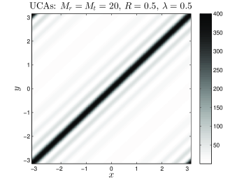
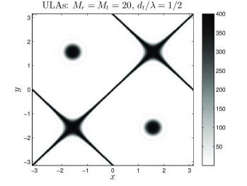
Refer to caption
(a)
Refer to caption
(b)
Figure 4: The function |ฯ†tโ€‹(r)(x,y|๐”—(โ„œ))|2\left|\varphi_{t\left(r\right)}\left(x,y\left|\mathfrak{T}\left(\mathfrak{R}\right)\right.\right)\right|^{2} of Example 1 with respect to (x,y)โˆˆ[โˆ’ฯ€,ฯ€]2๐‘ฅ๐‘ฆsuperscript๐œ‹๐œ‹2\left(x,y\right)\in\left[-\pi,\pi\right]^{2} (just for visualization purposes) for the case of (a) a symmetric UCA pair and (b) a symmetric ULA pair.
Example 1.

Consider a MIMO Radar system equipped (for simplicity) with identical Uniform Circular Arrays (UCAs) with Mr=Mt=20โ‰œMsubscript๐‘€๐‘Ÿsubscript๐‘€๐‘ก20โ‰œ๐‘€M_{r}=M_{t}=20\triangleq M antennas, whose positions in the 222-dimensional plane are defined as

[xltโ€‹(r)yltโ€‹(r)]โ‰œRโ€‹[cosโก(2โ€‹ฯ€โ€‹(lโˆ’1)M)sinโก(2โ€‹ฯ€โ€‹(lโˆ’1)M)],โ‰œmatrixsuperscriptsubscript๐‘ฅ๐‘™๐‘ก๐‘Ÿsuperscriptsubscript๐‘ฆ๐‘™๐‘ก๐‘Ÿ๐‘…matrix2๐œ‹๐‘™1๐‘€2๐œ‹๐‘™1๐‘€\begin{bmatrix}x_{l}^{t\left(r\right)}\\ y_{l}^{t\left(r\right)}\end{bmatrix}\triangleq R\begin{bmatrix}\cos\left(\dfrac{2\pi\left(l-1\right)}{M}\right)\\ \sin\left(\dfrac{2\pi\left(l-1\right)}{M}\right)\end{bmatrix}, (84)

lโˆˆโ„•Mโˆ’1๐‘™subscriptโ„•๐‘€1l\in\mathbb{N}_{M-1}, where R=0.5โ€‹m๐‘…0.5๐‘šR=0.5\,m. The wavelength utilized for the communication is chosen as ฮป=0.5โ€‹m๐œ†0.5๐‘š\lambda=0.5\,m. Then, Theorem 6 suggests that in order to bound the coherence of the respective matrix ๐šซ๐šซ\boldsymbol{\Delta}, a uniformly sampled version of which is available at the receiverโ€™s fusion center, we have to specify the supremum given by (75), which, of course, cannot be computed analytically. Fig. 4(a) shows the function |ฯ†tโ€‹(r)(x,y|๐”—(โ„œ))|2\left|\varphi_{t\left(r\right)}\left(x,y\left|\mathfrak{T}\left(\mathfrak{R}\right)\right.\right)\right|^{2} with respect to (x,y)โˆˆ[โˆ’ฯ€,ฯ€]2๐‘ฅ๐‘ฆsuperscript๐œ‹๐œ‹2\left(x,y\right)\in\left[-\pi,\pi\right]^{2}. We observe that this function is periodic in the 222-dimensional plane, with period equal to 2โ€‹ฯ€2๐œ‹2\pi in each dimension.

Let us now assume that

๐’œโ‰œ{(x,y)โˆˆ[โˆ’ฯ€2,ฯ€2]2|ฮทโ‰ค|yโˆ’x|โ‰คฯ€},โ‰œ๐’œconditional-set๐‘ฅ๐‘ฆsuperscript๐œ‹2๐œ‹22๐œ‚๐‘ฆ๐‘ฅ๐œ‹\mathcal{A}\triangleq\left\{\left.\left(x,y\right)\in\left[-\dfrac{\pi}{2},\dfrac{\pi}{2}\right]^{2}\right|\eta\leq\left|y-x\right|\leq\pi\right\}, (85)

for some ฮทโˆˆ(0,ฯ€)๐œ‚0๐œ‹\eta\in\left(0,\pi\right), that is, every pair of distinct angles ฮธisubscript๐œƒ๐‘–\theta_{i} and ฮธjsubscript๐œƒ๐‘—\theta_{j} are such that the magnitudes of their differences are lying in two non intersecting halfplanes, one above and one below the hyperplane y=x๐‘ฆ๐‘ฅy=x, within a margin of ฮท๐œ‚\eta.

Empirically, using the graph of |ฯ†tโ€‹(r)(x,y|๐”—(โ„œ))|2\left|\varphi_{t\left(r\right)}\left(x,y\left|\mathfrak{T}\left(\mathfrak{R}\right)\right.\right)\right|^{2}, we can easily specify its supremum over the set ๐’œ๐’œ\mathcal{A}, which is required in order to bound the coherence of ๐šซ๐šซ\boldsymbol{\Delta}. Additionally, it is obvious that if ฮท๐œ‚\eta is sufficiently large, the coherence of ๐šซ๐šซ\boldsymbol{\Delta} will be essentially relatively small.

Interestingly, this fact draws immediate connections regarding the coherence between the UCA and the ULA case (see Theorem 3 and Lemma 2). The function |ฯ†tโ€‹(r)(x,y|๐”—(โ„œ))|2\left|\varphi_{t\left(r\right)}\left(x,y\left|\mathfrak{T}\left(\mathfrak{R}\right)\right.\right)\right|^{2} resulting from the application of Theorem 6 for the ULA case is shown in Fig. 4(b). We observe that the sufficient condition for low coherence of ๐šซ๐šซ\boldsymbol{\Delta} presented in Lemma 2 can be immediately validated.

Comparing the two graphs shown in Fig. 4, we can infer that in the UCA case the allowable region for the magnitudes of the differences of the angle pairs, given by the set ๐’œ๐’œ\mathcal{A}, is larger than the respective region for the ULA case (Lemma 2). On the other hand, the values of |ฯ†tโ€‹(r)(x,y|๐”—(โ„œ))|2\left|\varphi_{t\left(r\right)}\left(x,y\left|\mathfrak{T}\left(\mathfrak{R}\right)\right.\right)\right|^{2} for the ULA case in the interior of the allowable region are considerably smaller than the values of the respective function in the interior of the respective set for the UCA case. Consequently, regarding our choice of transmission/reception arrays, there is an obvious trade - off between โ€œresolutionโ€ and coherence. โ– โ– \blacksquare

Remark 2.

There are other fancier types of 222-dimensional arrays that can achieve a much better โ€œresolution/coherence ratioโ€. For instance, we have found experimentally that carefully designed spiral arrays, whose antenna positions constitute a sampling of the usual Archimedean Spiral, possess the advantages of both the aforementioned cases and, additionally, they exhibit very good asymptotic properties, guaranteeing low coherence for a sufficiently large number of antennas.

V Coherence of ๐šซ๐šซ\boldsymbol{\Delta} for the case where
ฮธiโ‰กฮธjsubscript๐œƒ๐‘–subscript๐œƒ๐‘—\theta_{i}\equiv\theta_{j} for some (i,j)โˆˆโ„•Kโˆ’1ร—โ„•Kโˆ’1๐‘–๐‘—subscriptโ„•๐พ1subscriptโ„•๐พ1\left(i,j\right)\in\mathbb{N}_{K-1}\times\mathbb{N}_{K-1} with iโ‰ j๐‘–๐‘—i\neq j

Until now, in all the results we have presented, we have assumed that the target angles ฮธk,kโˆˆโ„•Kโˆ’1subscript๐œƒ๐‘˜๐‘˜subscriptโ„•๐พ1\theta_{k},k\in\mathbb{N}_{K-1} are almost surely distinct. Apparently, this required property of distinctness is far weaker than (statistical) independence. In fact, our results presented in detail in the previous sections continue to hold without any modification for any set of dependent target angles, as long as they are all different from each other with probability 111 (recall the Vandermonde/alternant structure of the matrices ๐—rsubscript๐—๐‘Ÿ\mathbf{X}_{r} and ๐—tsubscript๐—๐‘ก\mathbf{X}_{t} in the proofs of Theorems 3 and 6). Therefore, regarding the coherence of ๐šซ๐šซ\boldsymbol{\Delta} for arbitrary 222-dimensional arrays (and thus also for ULAs), the only case that needs special treatment is when ฮธiโ‰กฮธjsubscript๐œƒ๐‘–subscript๐œƒ๐‘—\theta_{i}\equiv\theta_{j} for some (i,j)โˆˆโ„•Kโˆ’1ร—โ„•Kโˆ’1๐‘–๐‘—subscriptโ„•๐พ1subscriptโ„•๐พ1\left(i,j\right)\in\mathbb{N}_{K-1}\times\mathbb{N}_{K-1} with iโ‰ j๐‘–๐‘—i\neq j, for which we present and prove the following result.

Theorem 7.

(Coherence for Non - Distinct Angles) Consider an arbitrary 222-dimensional array transmitter - receiver pair equipped with Mtsubscript๐‘€๐‘กM_{t} and Mrsubscript๐‘€๐‘ŸM_{r} antennas, respectively. Assume that the set of angles ฮ˜โ‰œ{ฮธk}kโˆˆโ„•Kโˆ’1โ‰œฮ˜subscriptsubscript๐œƒ๐‘˜๐‘˜subscriptโ„•๐พ1\Theta\triangleq\left\{\theta_{k}\right\}_{k\in\mathbb{N}_{K-1}} is such that it can be partitioned as

ฮ˜=๐’Ÿโ€‹โ‹ƒโ„›with๐’Ÿโ€‹โ‹‚โ„›โ‰กร˜,formulae-sequenceฮ˜๐’Ÿโ„›with๐’Ÿโ„›ร˜\Theta=\mathcal{D}\bigcup\mathcal{R}\quad\text{with}\quad\mathcal{D}\bigcap\mathcal{R}\equiv\textrm{\O}, (86)

where ๐’ŸโŠ†ฮ˜๐’Ÿฮ˜\mathcal{D}\subseteq\Theta contains almost surely distinct members and

โ„›โ‰œ{ฮธโˆˆฮ˜\๐’Ÿ|ฮธโ‰กฯโ€‹ย a.s.ย for someย โ€‹ฯโˆˆ๐’Ÿ}.โ‰œโ„›conditional-set๐œƒ\ฮ˜๐’Ÿ๐œƒ๐œŒย a.s.ย for someย ๐œŒ๐’Ÿ\mathcal{R}\triangleq\left\{\theta\in\Theta\backslash\mathcal{D}\left|\theta\equiv\rho\text{ a.s.}\text{ for some }\rho\in\mathcal{D}\right.\right\}. (87)

Let ๐šซ๐šซ\boldsymbol{\Delta} and ๐šซ๐’Ÿsubscript๐šซ๐’Ÿ\boldsymbol{\Delta}_{\mathcal{D}} be the matrices associated with the angle sets ฮ˜ฮ˜\Theta and ๐’Ÿ๐’Ÿ\mathcal{D}, respectively. Then, it is true that

ฮผโ€‹(U)โ€‹โ‰กa.s.โ€‹ฮผโ€‹(U๐’Ÿ)andฮผโ€‹(V)โ€‹โ‰กa.s.โ€‹ฮผโ€‹(V๐’Ÿ).๐œ‡๐‘ˆa.s.๐œ‡subscript๐‘ˆ๐’Ÿand๐œ‡๐‘‰a.s.๐œ‡subscript๐‘‰๐’Ÿ\mu\left(U\right)\overset{\text{a.s.}}{\equiv}\mu\left(U_{\mathcal{D}}\right)\quad\text{and}\quad\mu\left(V\right)\overset{\text{a.s.}}{\equiv}\mu\left(V_{\mathcal{D}}\right). (88)
Proof of Theorem 7.

Consider the matrix

๐šซ=๐—rโ€‹๐ƒ๐—t๐‘ปโˆˆโ„‚Mtร—Mr,๐šซsubscript๐—๐‘Ÿsuperscriptsubscript๐ƒ๐—๐‘ก๐‘ปsuperscriptโ„‚subscript๐‘€๐‘กsubscript๐‘€๐‘Ÿ\boldsymbol{\Delta}=\mathbf{X}_{r}\mathbf{D}\mathbf{X}_{t}^{\boldsymbol{T}}\in\mathbb{C}^{M_{t}\times M_{r}}, (89)

where ๐—rโˆˆโ„‚Mrร—Ksubscript๐—๐‘Ÿsuperscriptโ„‚subscript๐‘€๐‘Ÿ๐พ\mathbf{X}_{r}\in\mathbb{C}^{M_{r}\times K}, ๐—tโˆˆโ„‚Mtร—Ksubscript๐—๐‘กsuperscriptโ„‚subscript๐‘€๐‘ก๐พ\mathbf{X}_{t}\in\mathbb{C}^{M_{t}\times K} and ๐ƒโˆˆโ„‚Kร—K๐ƒsuperscriptโ„‚๐พ๐พ\mathbf{D}\in\mathbb{C}^{K\times K} are defined as in the proof of either Theorem 3 or Theorem 6. Let the assumptions of the statement of Theorem 7 hold true. Then, only |๐’Ÿ|โ‰œLโ‰œ๐’Ÿ๐ฟ\left|\mathcal{D}\right|\triangleq L columns of both ๐—rsubscript๐—๐‘Ÿ\mathbf{X}_{r} and ๐—tsubscript๐—๐‘ก\mathbf{X}_{t} will be almost surely linearly independent, whereas the rest |โ„›|โ‰กKโˆ’Lโ„›๐พ๐ฟ\left|\mathcal{R}\right|\equiv K-L columns of both matrices constitute repetitions of the aforementioned L๐ฟL ones. As a result, ๐šซ๐šซ\boldsymbol{\Delta} will be almost surely of rank L๐ฟL.

Let us re-express ๐šซ๐šซ\boldsymbol{\Delta} as

๐šซ=๐—~rโ€‹๐๐ƒ๐๐‘ปโ€‹๐—~t๐‘ปโ‰ก๐—~rโ€‹๐ƒ~โ€‹๐—~t๐‘ป,๐šซsubscript~๐—๐‘Ÿsuperscript๐๐ƒ๐๐‘ปsuperscriptsubscript~๐—๐‘ก๐‘ปsubscript~๐—๐‘Ÿ~๐ƒsuperscriptsubscript~๐—๐‘ก๐‘ป\boldsymbol{\Delta}=\widetilde{\mathbf{X}}_{r}\mathbf{P}\mathbf{D}\mathbf{P}^{\boldsymbol{T}}\widetilde{\mathbf{X}}_{t}^{\boldsymbol{T}}\equiv\widetilde{\mathbf{X}}_{r}\widetilde{\mathbf{D}}\widetilde{\mathbf{X}}_{t}^{\boldsymbol{T}}, (90)

where ๐โˆˆโ„Kร—K๐superscriptโ„๐พ๐พ\mathbf{P}\in\mathbb{R}^{K\times K} constitutes an appropriately chosen permutation matrix such that

๐—~rsubscript~๐—๐‘Ÿ\displaystyle\widetilde{\mathbf{X}}_{r} โ‰œ[๐—r๐’Ÿ๐—rโ„›]andโ‰œabsentdelimited-[]superscriptsubscript๐—๐‘Ÿ๐’Ÿsuperscriptsubscript๐—๐‘Ÿโ„›and\displaystyle\triangleq\left[\begin{array}[]{c|c}\mathbf{X}_{r}^{\mathcal{D}}&\mathbf{X}_{r}^{\mathcal{R}}\end{array}\right]\quad\text{and} (92)
๐—~tsubscript~๐—๐‘ก\displaystyle\widetilde{\mathbf{X}}_{t} โ‰œ[๐—t๐’Ÿ๐—tโ„›],โ‰œabsentdelimited-[]superscriptsubscript๐—๐‘ก๐’Ÿsuperscriptsubscript๐—๐‘กโ„›\displaystyle\triangleq\left[\begin{array}[]{c|c}\mathbf{X}_{t}^{\mathcal{D}}&\mathbf{X}_{t}^{\mathcal{R}}\end{array}\right], (94)

where ๐—r๐’Ÿโˆˆโ„‚Mrร—Lsuperscriptsubscript๐—๐‘Ÿ๐’Ÿsuperscriptโ„‚subscript๐‘€๐‘Ÿ๐ฟ\mathbf{X}_{r}^{\mathcal{D}}\in\mathbb{C}^{M_{r}\times L} (respectively for ๐—t๐’Ÿโˆˆโ„‚Mtร—Lsuperscriptsubscript๐—๐‘ก๐’Ÿsuperscriptโ„‚subscript๐‘€๐‘ก๐ฟ\mathbf{X}_{t}^{\mathcal{D}}\in\mathbb{C}^{M_{t}\times L}) contains the columns of ๐—rsubscript๐—๐‘Ÿ\mathbf{X}_{r} associated with the almost surely distinct angles in ๐’Ÿ๐’Ÿ\mathcal{D} and ๐—rโ„›โˆˆโ„‚Mrร—Kโˆ’Lsuperscriptsubscript๐—๐‘Ÿโ„›superscriptโ„‚subscript๐‘€๐‘Ÿ๐พ๐ฟ\mathbf{X}_{r}^{\mathcal{R}}\in\mathbb{C}^{M_{r}\times K-L} (respectively for ๐—tโ„›โˆˆโ„‚Mtร—Kโˆ’Lsuperscriptsubscript๐—๐‘กโ„›superscriptโ„‚subscript๐‘€๐‘ก๐พ๐ฟ\mathbf{X}_{t}^{\mathcal{R}}\in\mathbb{C}^{M_{t}\times K-L}) contains the rest of columns of ๐—rsubscript๐—๐‘Ÿ\mathbf{X}_{r}, associated with the rest of the angles in โ„›โ„›\mathcal{R}. Of course, ๐ƒ~โˆˆโ„‚Kร—K~๐ƒsuperscriptโ„‚๐พ๐พ\widetilde{\mathbf{D}}\in\mathbb{C}^{K\times K} constitutes a non - zero - diagonal matrix.

Respectively for ๐—~tsubscript~๐—๐‘ก\widetilde{\mathbf{X}}_{t}, the thin QR decomposition of ๐—~rsubscript~๐—๐‘Ÿ\widetilde{\mathbf{X}}_{r} can be expressed as

๐—~rsubscript~๐—๐‘Ÿ\displaystyle\widetilde{\mathbf{X}}_{r} =๐•~rโ€‹๐€~rabsentsubscript~๐•๐‘Ÿsubscript~๐€๐‘Ÿ\displaystyle=\widetilde{\mathbf{V}}_{r}\widetilde{\mathbf{A}}_{r}
โ‰œ[๐•r๐’Ÿ๐•rโ„›]โ€‹[๐€r๐’Ÿ๐ŸŽ]โ‰œabsentdelimited-[]superscriptsubscript๐•๐‘Ÿ๐’Ÿsuperscriptsubscript๐•๐‘Ÿโ„›delimited-[]superscriptsubscript๐€๐‘Ÿ๐’Ÿmissing-subexpression0\displaystyle\triangleq\left[\begin{array}[]{c|c}\mathbf{V}_{r}^{\mathcal{D}}&\mathbf{V}_{r}^{\mathcal{R}}\end{array}\right]\left[\begin{array}[]{c}\mathbf{A}_{r}^{\mathcal{D}}\\ \hline\cr\mathbf{0}\end{array}\right] (98)
โ‰ก๐•r๐’Ÿโ€‹๐€r๐’Ÿ,absentsuperscriptsubscript๐•๐‘Ÿ๐’Ÿsuperscriptsubscript๐€๐‘Ÿ๐’Ÿ\displaystyle\equiv\mathbf{V}_{r}^{\mathcal{D}}\mathbf{A}_{r}^{\mathcal{D}}, (99)

where ๐•~rโˆˆโ„‚Mrร—Ksubscript~๐•๐‘Ÿsuperscriptโ„‚subscript๐‘€๐‘Ÿ๐พ\widetilde{\mathbf{V}}_{r}\in\mathbb{C}^{M_{r}\times K} is such that ๐•~r๐‘ฏโ€‹๐•~rโ‰ก๐ˆKsuperscriptsubscript~๐•๐‘Ÿ๐‘ฏsubscript~๐•๐‘Ÿsubscript๐ˆ๐พ\widetilde{\mathbf{V}}_{r}^{\boldsymbol{\mathit{H}}}\widetilde{\mathbf{V}}_{r}\equiv\mathbf{I}_{K}, ๐•r๐’Ÿโˆˆโ„‚Mrร—Lsuperscriptsubscript๐•๐‘Ÿ๐’Ÿsuperscriptโ„‚subscript๐‘€๐‘Ÿ๐ฟ\mathbf{V}_{r}^{\mathcal{D}}\in\mathbb{C}^{M_{r}\times L} is such that (๐•r๐’Ÿ)๐‘ฏโ€‹๐•r๐’Ÿโ‰ก๐ˆLsuperscriptsuperscriptsubscript๐•๐‘Ÿ๐’Ÿ๐‘ฏsuperscriptsubscript๐•๐‘Ÿ๐’Ÿsubscript๐ˆ๐ฟ\left(\mathbf{V}_{r}^{\mathcal{D}}\right)^{\boldsymbol{\mathit{H}}}\mathbf{V}_{r}^{\mathcal{D}}\equiv\mathbf{I}_{L}, ๐€~rโˆˆโ„‚Kร—Ksubscript~๐€๐‘Ÿsuperscriptโ„‚๐พ๐พ\widetilde{\mathbf{A}}_{r}\in\mathbb{C}^{K\times K} is a specially structured singular upper triangular matrix (see expressions above) of rank L๐ฟL and ๐€r๐’Ÿโˆˆโ„‚Lร—Ksuperscriptsubscript๐€๐‘Ÿ๐’Ÿsuperscriptโ„‚๐ฟ๐พ\mathbf{A}_{r}^{\mathcal{D}}\in\mathbb{C}^{L\times K} constitutes a rectangular matrix also of rank L๐ฟL.

Let (๐•rโ€‹(t)๐’Ÿ)iโˆˆโ„‚1ร—Lsuperscriptsuperscriptsubscript๐•๐‘Ÿ๐‘ก๐’Ÿ๐‘–superscriptโ„‚1๐ฟ\left(\mathbf{V}_{r\left(t\right)}^{\mathcal{D}}\right)^{i}\in\mathbb{C}^{1\times L}, iโˆˆโ„•Mrโ€‹(t)+๐‘–superscriptsubscriptโ„•subscript๐‘€๐‘Ÿ๐‘กi\in\mathbb{N}_{M_{r\left(t\right)}}^{+} denote the i๐‘–i-th row of ๐•rโ€‹(t)๐’Ÿsuperscriptsubscript๐•๐‘Ÿ๐‘ก๐’Ÿ\mathbf{V}_{r\left(t\right)}^{\mathcal{D}}. Then, based on (99) and using an almost identical procedure as in the first part of the proof of Theorem 3, we can directly show that the coherence of the column space of ๐šซ๐šซ\boldsymbol{\Delta}, U๐‘ˆU, is given by

ฮผโ€‹(U)๐œ‡๐‘ˆ\displaystyle\mu\left(U\right) =MrLโ€‹supiโˆˆโ„•N+โ€–(๐•r๐’Ÿ)iโ€–22.absentsubscript๐‘€๐‘Ÿ๐ฟsubscriptsupremum๐‘–superscriptsubscriptโ„•๐‘superscriptsubscriptnormsuperscriptsuperscriptsubscript๐•๐‘Ÿ๐’Ÿ๐‘–22\displaystyle=\frac{M_{r}}{L}\sup_{i\in\mathbb{N}_{N}^{+}}\left\|\left(\mathbf{V}_{r}^{\mathcal{D}}\right)^{i}\right\|_{2}^{2}. (100)

Respectively, the coherence of the row space of of ๐šซ๐šซ\boldsymbol{\Delta}, V๐‘‰V, is given by

ฮผโ€‹(V)=MtLโ€‹supiโˆˆโ„•N+โ€–(๐•t๐’Ÿ)iโ€–22.๐œ‡๐‘‰subscript๐‘€๐‘ก๐ฟsubscriptsupremum๐‘–superscriptsubscriptโ„•๐‘superscriptsubscriptnormsuperscriptsuperscriptsubscript๐•๐‘ก๐’Ÿ๐‘–22\mu\left(V\right)=\frac{M_{t}}{L}\sup_{i\in\mathbb{N}_{N}^{+}}\left\|\left(\mathbf{V}_{t}^{\mathcal{D}}\right)^{i}\right\|_{2}^{2}. (101)

Now, consider the almost surely rank-L๐ฟL matrix

๐šซ๐’Ÿโ‰œ๐—r๐’Ÿโ€‹๐ƒ๐’Ÿโ€‹๐—t๐’Ÿโˆˆโ„‚Mtร—Mr,โ‰œsubscript๐šซ๐’Ÿsuperscriptsubscript๐—๐‘Ÿ๐’Ÿsuperscript๐ƒ๐’Ÿsuperscriptsubscript๐—๐‘ก๐’Ÿsuperscriptโ„‚subscript๐‘€๐‘กsubscript๐‘€๐‘Ÿ\boldsymbol{\Delta}_{\mathcal{D}}\triangleq\mathbf{X}_{r}^{\mathcal{D}}\mathbf{D}^{\mathcal{D}}\mathbf{X}_{t}^{\mathcal{D}}\in\mathbb{C}^{M_{t}\times M_{r}}, (102)

where the diagonal matrix ๐ƒ๐’Ÿโˆˆโ„‚Lร—Lsuperscript๐ƒ๐’Ÿsuperscriptโ„‚๐ฟ๐ฟ\mathbf{D}^{\mathcal{D}}\in\mathbb{C}^{L\times L} is defined in an obvious way (see (90) - (94)). Then, by construction of the QR decomposition, it must be true that

๐—r๐’Ÿ=๐•r๐’Ÿโ€‹๐€^r๐’Ÿand๐—t๐’Ÿ=๐•t๐’Ÿโ€‹๐€^t๐’Ÿ,formulae-sequencesuperscriptsubscript๐—๐‘Ÿ๐’Ÿsuperscriptsubscript๐•๐‘Ÿ๐’Ÿsuperscriptsubscript^๐€๐‘Ÿ๐’Ÿandsuperscriptsubscript๐—๐‘ก๐’Ÿsuperscriptsubscript๐•๐‘ก๐’Ÿsuperscriptsubscript^๐€๐‘ก๐’Ÿ\mathbf{X}_{r}^{\mathcal{D}}=\mathbf{V}_{r}^{\mathcal{D}}\widehat{\mathbf{A}}_{r}^{\mathcal{D}}\quad\text{and}\quad\mathbf{X}_{t}^{\mathcal{D}}=\mathbf{V}_{t}^{\mathcal{D}}\widehat{\mathbf{A}}_{t}^{\mathcal{D}}, (103)

where, ๐€^t๐’Ÿโˆˆโ„‚Lร—Lsuperscriptsubscript^๐€๐‘ก๐’Ÿsuperscriptโ„‚๐ฟ๐ฟ\widehat{\mathbf{A}}_{t}^{\mathcal{D}}\in\mathbb{C}^{L\times L} and ๐€^r๐’Ÿโˆˆโ„‚Lร—Lsuperscriptsubscript^๐€๐‘Ÿ๐’Ÿsuperscriptโ„‚๐ฟ๐ฟ\widehat{\mathbf{A}}_{r}^{\mathcal{D}}\in\mathbb{C}^{L\times L} constitute almost surely full rank matrices. Recall (38) and adapt it appropriately for expressing the coherences of the column and row spaces of ๐šซ๐’Ÿsubscript๐šซ๐’Ÿ\boldsymbol{\Delta}_{\mathcal{D}}, U๐’Ÿsubscript๐‘ˆ๐’ŸU_{\mathcal{D}} and V๐’Ÿsubscript๐‘‰๐’ŸV_{\mathcal{D}}, respectively. Our claims follow.โˆŽ

Remark 3.

Indeed, in many applications (Radar and non - Radar), it is very likely that the situations Theorem 7 is dealing with may correspond to events of zero measure. However, we feel that stating this result is important, in order for the coherence analysis we presented in the previous chapters to be entirely complete. Also, interestingly, the simple implication of Theorem 7 is somewhat not intuitive: As the difference between two angles is decreasing, the coherence of ๐šซ๐šซ\boldsymbol{\Delta} becomes worse (that is, increases), but if the difference is exactly zero, then the coherence of ๐šซ๐šซ\boldsymbol{\Delta} is identical to the coherence of the variation of ๐šซ๐šซ\boldsymbol{\Delta} resulting from simply removing the information corresponding to any of the two identical angles. Clearly, this result does not in any way contradict the ones presented in the previous sections.

VI Discussion and Some Simulations

In this section, we present some simulations, validating our main results presented above and discuss some further implications of our respective theoretical analysis.

For simplicity, we consider a MIMO radar system equipped with identical ULAs for transmission and reception, with drโ‰กdt=ฮป/2subscript๐‘‘๐‘Ÿsubscript๐‘‘๐‘ก๐œ†2d_{r}\equiv d_{t}=\lambda/2 and Mrโ‰กMtโ‰œMsubscript๐‘€๐‘Ÿsubscript๐‘€๐‘กโ‰œ๐‘€M_{r}\equiv M_{t}\triangleq M. We also consider K=4๐พ4K=4 targets in the far field, with angles independently distributed in (โˆ’ฯ€2,ฯ€2)๐œ‹2๐œ‹2\left(-\dfrac{\pi}{2},\dfrac{\pi}{2}\right).

Refer to caption
Figure 5: Behavior of the coherence of ๐šซ๐šซ\boldsymbol{\Delta} and the proposed bound with respect to the number of antennas M๐‘€M.

In this synthetic example, in order to demonstrate the validity of Theorem 3, we assume that the target angles are known apriori. By Lemma 2, we know that the condition ฮพโ‰ 0๐œ‰0\xi\neq 0 will always hold and consequently the asymptotics of Theorem 3 must also hold true. Of course, ฮพ๐œ‰\xi can be computed either using (24) or (66) (for some sufficiently chosen value of ฮท๐œ‚\eta), with the latter producing a worst - case bound regarding the coherence of the associated matrix ๐šซ๐šซ\boldsymbol{\Delta}. Also, in this example, we obviously have ฮผโ€‹(U)โ‰กฮผโ€‹(V)๐œ‡๐‘ˆ๐œ‡๐‘‰\mu\left(U\right)\equiv\mu\left(V\right).

Using (24) for the computation of ฮพ๐œ‰\xi, Fig. 5 shows the behavior of both the coherence of ๐šซ๐šซ\boldsymbol{\Delta} and its bound ฮผ0subscript๐œ‡0\mu_{0}, which results by directly applying Theorem 3, as a function of the number of transmission/reception antennas M๐‘€M. We observe that, clearly, the proposed bound is tight and it tracks the convergence of the coherence of ๐šซ๐šซ\boldsymbol{\Delta} to unity very accurately. We should mention here that for very small angle differences, the bound becomes somewhat looser. However, our numerical simulations have shown that our bound constitutes a very reasonable coherence estimate in all cases.
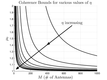
Refer to caption
Figure 6: Our proposed bound with respect to the number of antennas M๐‘€M, for different values of ฮท๐œ‚\eta, according to Lemma 2.

Apparently, in any realistic situation, the actual values of the target angles are unknown. Assuming generically that each of the angle differences belongs to a set given by (65) for some ฮทโˆˆ(0,ฯ€2)๐œ‚0๐œ‹2\eta\in\left(0,\dfrac{\pi}{2}\right) -ฮท๐œ‚\eta depends on the specific radar application-, we can invoke Lemma 2 in order to bound the coherence of ๐šซ๐šซ\boldsymbol{\Delta} in this more general case. Fig. 6 depicts a number of bounds produced by Lemma 2 for various values of ฮท๐œ‚\eta, as functions of the number of antennas M๐‘€M. One can observe that, as the value of ฮท๐œ‚\eta increases, the respective coherence bound converges much faster to unity, therefore increasing our confidence that the performance of matrix completion will be satisfactory for a relatively smaller number of transmission/reception antennas.
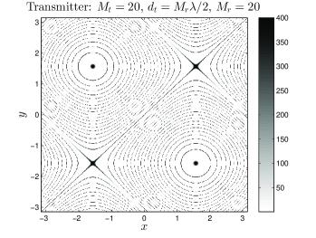
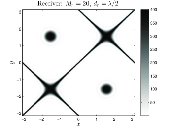
Refer to caption
(a)
Refer to caption
(b)
Figure 7: The function |ฯ†tโ€‹(r)(x,y|๐”—(โ„œ))|2\left|\varphi_{t\left(r\right)}\left(x,y\left|\mathfrak{T}\left(\mathfrak{R}\right)\right.\right)\right|^{2} with respect to (x,y)โˆˆ[โˆ’ฯ€,ฯ€]2๐‘ฅ๐‘ฆsuperscript๐œ‹๐œ‹2\left(x,y\right)\in\left[-\pi,\pi\right]^{2} for (a) the transmission array (๐”—๐”—\mathfrak{T}) and (b) the reception array (โ„œโ„œ\mathfrak{R}) of the high degree of freedom MIMO radar considered in this case.

However, we should stress that Lemma 2 essentially produces worst case bounds, which might be too pessimistic for specific applications. If this is the case, one could use Theorem 6, which provides greater versatility for deriving more accurate bounds for more specific target configurations and for given number of antennas or, alternatively, one could derive variants of Lemma 2 for special target configurations.

Another important ULA configuration in MIMO radar systems results by choosing dt=Mrโ€‹ฮป/2subscript๐‘‘๐‘กsubscript๐‘€๐‘Ÿ๐œ†2d_{t}=M_{r}\lambda/2 and dr=ฮป/2subscript๐‘‘๐‘Ÿ๐œ†2d_{r}=\lambda/2. It is well known that this particular choice for the transmitter antenna spacing increases the degrees of freedom of the system to Mtโ€‹Mrsubscript๐‘€๐‘กsubscript๐‘€๐‘ŸM_{t}M_{r} using only Mt+Mrsubscript๐‘€๐‘กsubscript๐‘€๐‘ŸM_{t}+M_{r} physical antenna elements and consequently, higher spatial resolution can be obtained (see, for instance, [18]). If we are interested in the performance of matrix completion, as far as ฮผโ€‹(V)๐œ‡๐‘‰\mu\left(V\right) is concerned, associated solely with the reception array, we can directly use Theorem 3 in conjunction with Lemma 2 as explained above in order to derive the respective coherence bound. However, the behavior of ฮผโ€‹(U)๐œ‡๐‘ˆ\mu\left(U\right) is much more complicated and the application of Theorem 3 leads to an unreasonably involved analysis. But one could invoke Theorem 6 in this case. Fig. 7(a) shows the function |ฯ†t(x,y|๐”—)|2\left|\varphi_{t}\left(x,y\left|\mathfrak{T}\right.\right)\right|^{2} with respect to (x,y)โˆˆ[โˆ’ฯ€,ฯ€]2๐‘ฅ๐‘ฆsuperscript๐œ‹๐œ‹2\left(x,y\right)\in\left[-\pi,\pi\right]^{2}. Assuming that the angles are independently and uniformly distributed in (โˆ’ฯ€2,ฯ€2)๐œ‹2๐œ‹2\left(-\dfrac{\pi}{2},\dfrac{\pi}{2}\right) and that the contours of |ฯ†t(x,y|๐”—)|2\left|\varphi_{t}\left(x,y\left|\mathfrak{T}\right.\right)\right|^{2} are sufficiently dense (for Mrsubscript๐‘€๐‘ŸM_{r} properly chosen), then the respective values of the aforementioned function will be essentially small, since, technically speaking, the probability of any (ฮธi,ฮธj)subscript๐œƒ๐‘–subscript๐œƒ๐‘—\left(\theta_{i},\theta_{j}\right) belonging to the union of the strict subsets of (โˆ’ฯ€2,ฯ€2)2superscript๐œ‹2๐œ‹22\left(-\dfrac{\pi}{2},\dfrac{\pi}{2}\right)^{2} corresponding to the contours of |ฯ†t(x,y|๐”—)|2\left|\varphi_{t}\left(x,y\left|\mathfrak{T}\right.\right)\right|^{2} shown in Fig. 7(a) will be essentially zero. Therefore, a low value for ฮผโ€‹(U)๐œ‡๐‘ˆ\mu\left(U\right) is guaranteed with very high probability.

VII Conclusion

In this paper, we have presented a detailed analysis regarding the recoverability of the data matrix in colocated MIMO radar systems via convex optimization (matrix completion), for a number of commonly used array configurations. We showed that, in most cases, the data matrix is indeed recoverable from a minimal number of observations, as long as the number of transmission and reception antennas is sufficiently large and under common assumptions on the DOAs of the targets. Consequently, the matrix completion approach for reducing the sampling requirements in colocated MIMO radar is indeed theoretically robust and also appealing for practical consideration in real world applications. However, although we have explicitly shown that the choice of ULAs for transmission and reception leads to asymptotically and approximately optimal coherence of the data matrix, the important and more general problem of optimally choosing the array topologies for minimizing matrix coherence still remains open, clearly suggesting new directions for further research.

Appendix A
Proof of Lemma 1

Let the hypothesis of the statement of Lemma 1 hold true. In the following, we consider only the column space of ๐Œ๐Œ\mathbf{M}, U๐‘ˆU, since, for V๐‘‰V the procedure is identical. First, consider the set ๐’ขโ‰œ{(i,j)โˆˆโ„•N+ร—โ„•N+|iโ‰กj}โ‰œ๐’ขconditional-set๐‘–๐‘—superscriptsubscriptโ„•๐‘superscriptsubscriptโ„•๐‘๐‘–๐‘—\mathcal{G}\triangleq\left\{\left(i,j\right)\in\mathbb{N}_{N}^{+}\times\mathbb{N}_{N}^{+}\left|i\equiv j\right.\right\}. Then,

sup(i,j)โˆˆ๐’ข|Nrโ€‹โŸจ๐ži,๐Uโ€‹๐žjโŸฉโˆ’๐Ÿ™i=j|subscriptsupremum๐‘–๐‘—๐’ข๐‘๐‘Ÿsubscript๐ž๐‘–subscript๐๐‘ˆsubscript๐ž๐‘—subscript1๐‘–๐‘—\displaystyle\sup_{\left(i,j\right)\in\mathcal{G}}\left|\frac{N}{r}\left\langle\mathbf{e}_{i},\mathbf{P}_{U}\mathbf{e}_{j}\right\rangle-\mathds{1}_{i=j}\right|
โ‰ก\displaystyle\equiv supiโˆˆโ„•N+Nrโ€‹โ€–๐Uโ€‹๐žiโ€–22โˆ’1โ‰คฮผ0โˆ’1.subscriptsupremum๐‘–superscriptsubscriptโ„•๐‘๐‘๐‘Ÿsuperscriptsubscriptnormsubscript๐๐‘ˆsubscript๐ž๐‘–221subscript๐œ‡01\displaystyle\sup_{i\in\mathbb{N}_{N}^{+}}\frac{N}{r}\left\|\mathbf{P}_{U}\mathbf{e}_{i}\right\|_{2}^{2}-1\leq\mu_{0}-1. (104)

Next, consider the set โ„‹โ‰œโ„•N+ร—โ„•N+โˆ’๐’ขโ‰œโ„‹superscriptsubscriptโ„•๐‘superscriptsubscriptโ„•๐‘๐’ข\mathcal{H}\triangleq\mathbb{N}_{N}^{+}\times\mathbb{N}_{N}^{+}-\mathcal{G}. In this case,

sup(i,j)โˆˆโ„‹|Nrโ€‹โŸจ๐ži,๐Uโ€‹๐žjโŸฉโˆ’๐Ÿ™i=j|subscriptsupremum๐‘–๐‘—โ„‹๐‘๐‘Ÿsubscript๐ž๐‘–subscript๐๐‘ˆsubscript๐ž๐‘—subscript1๐‘–๐‘—\displaystyle\sup_{\left(i,j\right)\in\mathcal{H}}\left|\frac{N}{r}\left\langle\mathbf{e}_{i},\mathbf{P}_{U}\mathbf{e}_{j}\right\rangle-\mathds{1}_{i=j}\right|
โ‰ก\displaystyle\equiv sup(i,j)โˆˆโ„‹Nrโ€‹|โŸจ๐Uโ€‹๐ži,๐Uโ€‹๐žjโŸฉ|subscriptsupremum๐‘–๐‘—โ„‹๐‘๐‘Ÿsubscript๐๐‘ˆsubscript๐ž๐‘–subscript๐๐‘ˆsubscript๐ž๐‘—\displaystyle\sup_{\left(i,j\right)\in\mathcal{H}}\frac{N}{r}\left|\left\langle\mathbf{P}_{U}\mathbf{e}_{i},\mathbf{P}_{U}\mathbf{e}_{j}\right\rangle\right|
โ‰ค\displaystyle\leq sup(i,j)โˆˆโ„‹Nrโ€‹โ€–๐Uโ€‹๐žiโ€–2โ€‹โ€–๐Uโ€‹๐žjโ€–2โ‰คฮผ0.subscriptsupremum๐‘–๐‘—โ„‹๐‘๐‘Ÿsubscriptnormsubscript๐๐‘ˆsubscript๐ž๐‘–2subscriptnormsubscript๐๐‘ˆsubscript๐ž๐‘—2subscript๐œ‡0\displaystyle\sup_{\left(i,j\right)\in\mathcal{H}}\frac{N}{r}\left\|\mathbf{P}_{U}\mathbf{e}_{i}\right\|_{2}\left\|\mathbf{P}_{U}\mathbf{e}_{j}\right\|_{2}\leq\mu_{0}. (105)

In all cases, it is true that

ฮผsโ€‹(U)โ‰คฮผ0andฮผsโ€‹(V)โ‰คฮผ0.formulae-sequencesubscript๐œ‡๐‘ ๐‘ˆsubscript๐œ‡0andsubscript๐œ‡๐‘ ๐‘‰subscript๐œ‡0\mu_{s}\left(U\right)\leq\mu_{0}\quad\text{and}\quad\mu_{s}\left(V\right)\leq\mu_{0}. (106)

Consequently, the assumption ๐€๐Ÿ๐€๐Ÿ\mathbf{A2} is trivially satisfied with

maxโก{ฮผsโ€‹(U),ฮผsโ€‹(V)}โ‰คฮผ0subscript๐œ‡๐‘ ๐‘ˆsubscript๐œ‡๐‘ ๐‘‰subscript๐œ‡0\max\left\{\mu_{s}\left(U\right),\mu_{s}\left(V\right)\right\}\leq\mu_{0} (107)

and then we can take ฮผ0sโ‰คฮผ0โ€‹rsuperscriptsubscript๐œ‡0๐‘ subscript๐œ‡0๐‘Ÿ\mu_{0}^{s}\leq\mu_{0}\sqrt{r}. Also, ฮผ1โ‰คฮผ0โ€‹rsubscript๐œ‡1subscript๐œ‡0๐‘Ÿ\mu_{1}\leq\mu_{0}\sqrt{r} [4, 5]. Choosing ฮผโ‰œmaxโก{ฮผ0s,ฮผ1}โ‰œ๐œ‡superscriptsubscript๐œ‡0๐‘ subscript๐œ‡1\mu\triangleq\max\left\{\mu_{0}^{s},\mu_{1}\right\} completes the proof. โˆŽ

Appendix B
Proof of Lemma 2

Let the hypotheses of the statement of Lemma 2 hold true and consider a bivariate function f:๐’œโ†’โ„ฑโŠ‚(0,2):๐‘“โ†’๐’œโ„ฑ02f:\mathcal{A}\rightarrow\mathcal{F}\subset\left(0,2\right) defined as

fโ€‹(x,y)โ‰œ|sinโก(x)โˆ’sinโก(y)|,โ‰œ๐‘“๐‘ฅ๐‘ฆ๐‘ฅ๐‘ฆf\left(x,y\right)\triangleq\left|\sin\left(x\right)-\sin\left(y\right)\right|, (108)

obviously bounded from above and below as

inf(x,y)โˆˆ๐’œfโ€‹(x,y)โ‰คfโ€‹(x,y)โ‰คsup(x,y)โˆˆ๐’œfโ€‹(x,y).subscriptinfimum๐‘ฅ๐‘ฆ๐’œ๐‘“๐‘ฅ๐‘ฆ๐‘“๐‘ฅ๐‘ฆsubscriptsupremum๐‘ฅ๐‘ฆ๐’œ๐‘“๐‘ฅ๐‘ฆ\inf_{\left(x,y\right)\in\mathcal{A}}f\left(x,y\right)\leq f\left(x,y\right)\leq\sup_{\left(x,y\right)\in\mathcal{A}}f\left(x,y\right). (109)

In the following, our goal will be to explicitly specify the infimum and the supremum appearing in (109), or equivalently the set โ„ฑโ„ฑ\mathcal{F}.

Consider the case where (x,y)โˆˆ{(x,y)โˆˆ๐’œ|y>x}โ‰œ๐’œ+๐‘ฅ๐‘ฆconditional-set๐‘ฅ๐‘ฆ๐’œ๐‘ฆ๐‘ฅโ‰œsubscript๐’œ\left(x,y\right)\in\left\{\left(x,y\right)\in\mathcal{A}\left|y>x\right.\right\}\triangleq\mathcal{A}_{+}. Thus,

fโ€‹(x,y)=sinโก(y)โˆ’sinโก(x)โ‰œf+โ€‹(x,y).๐‘“๐‘ฅ๐‘ฆ๐‘ฆ๐‘ฅโ‰œsubscript๐‘“๐‘ฅ๐‘ฆf\left(x,y\right)=\sin\left(y\right)-\sin\left(x\right)\triangleq f_{+}\left(x,y\right). (110)

Also, let us define the set

โ„’ฮฒโ‰œ{(x,y)โˆˆ๐’œ+|y=x+ฮฒ,ฮฒโˆˆ[ฮท,ฯ€โˆ’ฮท]}.โ‰œsubscriptโ„’๐›ฝconditional-set๐‘ฅ๐‘ฆsubscript๐’œformulae-sequence๐‘ฆ๐‘ฅ๐›ฝ๐›ฝ๐œ‚๐œ‹๐œ‚\mathcal{L}_{\beta}\triangleq\left\{\left(x,y\right)\in\mathcal{A}_{+}\left|y=x+\beta,\beta\in\left[\eta,\pi-\eta\right]\right.\right\}. (111)

Then, restricted to โ„’ฮฒsubscriptโ„’๐›ฝ\mathcal{L}_{\beta}, the function f+โ€‹(x,y)subscript๐‘“๐‘ฅ๐‘ฆf_{+}\left(x,y\right) can be expressed as

f+โ€‹(x,x+ฮฒ)=sinโก(x+ฮฒ)โˆ’sinโก(x)โ‰œf+โ€‹(x;ฮฒ),subscript๐‘“๐‘ฅ๐‘ฅ๐›ฝ๐‘ฅ๐›ฝ๐‘ฅโ‰œsubscript๐‘“๐‘ฅ๐›ฝf_{+}\left(x,x+\beta\right)=\sin\left(x+\beta\right)-\sin\left(x\right)\triangleq f_{+}\left(x;\beta\right), (112)

where xโˆˆ[โˆ’ฯ€2,ฯ€2โˆ’ฮฒ]๐‘ฅ๐œ‹2๐œ‹2๐›ฝx\in\left[-\dfrac{\pi}{2},\dfrac{\pi}{2}-\beta\right]. By a simple second derivative test, it can be shown that f+โ€‹(x;ฮฒ)subscript๐‘“๐‘ฅ๐›ฝf_{+}\left(x;\beta\right) is a strictly concave function in the set that it is defined. It is then very easy to show that f+โ€‹(x;ฮฒ)subscript๐‘“๐‘ฅ๐›ฝf_{+}\left(x;\beta\right) is maximized at x^โ‰กโˆ’ฮฒ2^๐‘ฅ๐›ฝ2\widehat{x}\equiv-\dfrac{\beta}{2} over the set [โˆ’ฯ€2,ฯ€2โˆ’ฮฒ]๐œ‹2๐œ‹2๐›ฝ\left[-\dfrac{\pi}{2},\dfrac{\pi}{2}-\beta\right], whereas its infimum occurs at either of the boundaries of the feasible set, say, at x~โ‰กโˆ’ฯ€2~๐‘ฅ๐œ‹2\widetilde{x}\equiv-\dfrac{\pi}{2}. Thus, trivially, the maximum of f+โ€‹(x,y)subscript๐‘“๐‘ฅ๐‘ฆf_{+}\left(x,y\right) over the set โ„’ฮฒsubscriptโ„’๐›ฝ\mathcal{L}_{\beta} occurs at the point

(x^,y^)^๐‘ฅ^๐‘ฆ\displaystyle\left(\widehat{x},\widehat{y}\right) โ‰ก(โˆ’ฮฒ2,ฮฒ2),withabsent๐›ฝ2๐›ฝ2with\displaystyle\equiv\left(-\dfrac{\beta}{2},\dfrac{\beta}{2}\right),\quad\text{with} (113)
max(x,y)โˆˆโ„’ฮฒโกf+โ€‹(x,y)subscript๐‘ฅ๐‘ฆsubscriptโ„’๐›ฝsubscript๐‘“๐‘ฅ๐‘ฆ\displaystyle\max_{\left(x,y\right)\in\mathcal{L}_{\beta}}f_{+}\left(x,y\right) โ‰ก2โ€‹sinโก(ฮฒ2),โˆ€ฮฒโˆˆ[ฮท,ฯ€โˆ’ฮท],formulae-sequenceabsent2๐›ฝ2for-all๐›ฝ๐œ‚๐œ‹๐œ‚\displaystyle\equiv 2\sin\left(\dfrac{\beta}{2}\right),\quad\forall\,\beta\in\left[\eta,\pi-\eta\right], (114)

whereas its infimum occurs at

(x~,y~)~๐‘ฅ~๐‘ฆ\displaystyle\left(\widetilde{x},\widetilde{y}\right) โ‰ก(โˆ’ฯ€2,ฮฒโˆ’ฯ€2),withabsent๐œ‹2๐›ฝ๐œ‹2with\displaystyle\equiv\left(-\dfrac{\pi}{2},\beta-\dfrac{\pi}{2}\right),\quad\text{with} (115)
inf(x,y)โˆˆโ„’ฮฒf+โ€‹(x,y)subscriptinfimum๐‘ฅ๐‘ฆsubscriptโ„’๐›ฝsubscript๐‘“๐‘ฅ๐‘ฆ\displaystyle\inf_{\left(x,y\right)\in\mathcal{L}_{\beta}}f_{+}\left(x,y\right) โ‰ก1โˆ’cosโก(ฮฒ),โˆ€ฮฒโˆˆ[ฮท,ฯ€โˆ’ฮท].formulae-sequenceabsent1๐›ฝfor-all๐›ฝ๐œ‚๐œ‹๐œ‚\displaystyle\equiv 1-\cos\left(\beta\right),\quad\forall\,\beta\in\left[\eta,\pi-\eta\right]. (116)

Apparently, both the maximum and infimum of f+โ€‹(x,y)subscript๐‘“๐‘ฅ๐‘ฆf_{+}\left(x,y\right) over โ„’ฮฒsubscriptโ„’๐›ฝ\mathcal{L}_{\beta} constitute strictly increasing functions of ฮฒ๐›ฝ\beta, which directly implies that

sup(x,y)โˆˆ๐’œ+f+โ€‹(x,y)โ‰ก2โ€‹sinโก(ฯ€โˆ’ฮท2)โ‰ก2โ€‹cosโก(ฮท2)subscriptsupremum๐‘ฅ๐‘ฆsubscript๐’œsubscript๐‘“๐‘ฅ๐‘ฆ2๐œ‹๐œ‚22๐œ‚2\sup_{\left(x,y\right)\in\mathcal{A}_{+}}f_{+}\left(x,y\right)\equiv 2\sin\left(\dfrac{\pi-\eta}{2}\right)\equiv 2\cos\left(\dfrac{\eta}{2}\right) (117)

and

inf(x,y)โˆˆ๐’œ+f+โ€‹(x,y)โ‰ก1โˆ’cosโก(ฮท).subscriptinfimum๐‘ฅ๐‘ฆsubscript๐’œsubscript๐‘“๐‘ฅ๐‘ฆ1๐œ‚\inf_{\left(x,y\right)\in\mathcal{A}_{+}}f_{+}\left(x,y\right)\equiv 1-\cos\left(\eta\right). (118)

Further, observe that fโ€‹(x,y)๐‘“๐‘ฅ๐‘ฆf\left(x,y\right) for (x,y)โˆˆ๐’œ๐‘ฅ๐‘ฆ๐’œ\left(x,y\right)\in\mathcal{A} is symmetric with respect to its main diagonal. Consequently, it must be true that

sup(x,y)โˆˆ๐’œfโ€‹(x,y)subscriptsupremum๐‘ฅ๐‘ฆ๐’œ๐‘“๐‘ฅ๐‘ฆ\displaystyle\sup_{\left(x,y\right)\in\mathcal{A}}f\left(x,y\right) โ‰ก2โ€‹cosโก(ฮท2)andabsent2๐œ‚2and\displaystyle\equiv 2\cos\left(\dfrac{\eta}{2}\right)\quad\text{and} (119)
inf(x,y)โˆˆ๐’œfโ€‹(x,y)subscriptinfimum๐‘ฅ๐‘ฆ๐’œ๐‘“๐‘ฅ๐‘ฆ\displaystyle\inf_{\left(x,y\right)\in\mathcal{A}}f\left(x,y\right) โ‰ก1โˆ’cosโก(ฮท),โˆ€ฮทโˆˆ(0,ฯ€2].formulae-sequenceabsent1๐œ‚for-all๐œ‚0๐œ‹2\displaystyle\equiv 1-\cos\left(\eta\right),\quad\forall\,\eta\in\left(0,\dfrac{\pi}{2}\right]. (120)

Therefore, โˆ€(x,y)โˆˆ๐’œfor-all๐‘ฅ๐‘ฆ๐’œ\forall\,\left(x,y\right)\in\mathcal{A},

fโ€‹(x,y)โˆˆ[1โˆ’cosโก(ฮท),2โ€‹cosโก(ฮท2)]โ‰กโ„ฑ.๐‘“๐‘ฅ๐‘ฆ1๐œ‚2๐œ‚2โ„ฑf\left(x,y\right)\in\left[1-\cos\left(\eta\right),2\cos\left(\dfrac{\eta}{2}\right)\right]\equiv\mathcal{F}. (121)

Now, substituting x๐‘ฅx and y๐‘ฆy with ฮธisubscript๐œƒ๐‘–\theta_{i} and ฮธjsubscript๐œƒ๐‘—\theta_{j}, respectively, (121) yields

1โˆ’cosโก(ฮท)2โ‰ค12โ€‹|sinโก(ฮธi)โˆ’sinโก(ฮธj)|โ‰คcosโก(ฮท2),1๐œ‚212subscript๐œƒ๐‘–subscript๐œƒ๐‘—๐œ‚2\dfrac{1-\cos\left(\eta\right)}{2}\leq\dfrac{1}{2}\left|\sin\left(\theta_{i}\right)-\sin\left(\theta_{j}\right)\right|\leq\cos\left(\dfrac{\eta}{2}\right), (122)

holding true โˆ€(i,j)โˆˆโ„•Kโˆ’1ร—โ„•Kโˆ’1for-all๐‘–๐‘—subscriptโ„•๐พ1subscriptโ„•๐พ1\forall\,\left(i,j\right)\in\mathbb{N}_{K-1}\times\mathbb{N}_{K-1} with iโ‰ j๐‘–๐‘—i\neq j and โˆ€ฮทโˆˆ(0,ฯ€2)for-all๐œ‚0๐œ‹2\forall\,\eta\in\left(0,\dfrac{\pi}{2}\right), where, in general,

1โˆ’cosโก(ฮท)21๐œ‚2\displaystyle\dfrac{1-\cos\left(\eta\right)}{2} โˆˆ(0,12]andabsent012and\displaystyle\in\left(0,\dfrac{1}{2}\right]\quad\text{and} (123)
cosโก(ฮท2)๐œ‚2\displaystyle\cos\left(\dfrac{\eta}{2}\right) โˆˆ[22,1).absent221\displaystyle\in\left[\dfrac{\sqrt{2}}{2},1\right). (124)

As a result, for a fixed ฮท๐œ‚\eta (recall the definition of ฮพ๐œ‰\xi in the statement of Theorem 3),

ฮพ๐œ‰\displaystyle\xi =min(i,j)โˆˆโ„•Kโˆ’1ร—โ„•Kโˆ’1iโ‰ jโกgโ€‹(12โ€‹|sinโก(ฮธi)โˆ’sinโก(ฮธj)|)absentsubscript๐‘–๐‘—subscriptโ„•๐พ1subscriptโ„•๐พ1๐‘–๐‘—๐‘”12subscript๐œƒ๐‘–subscript๐œƒ๐‘—\displaystyle=\min_{\begin{subarray}{c}\left(i,j\right)\in\mathbb{N}_{K-1}\times\mathbb{N}_{K-1}\\ i\neq j\end{subarray}}g\left(\dfrac{1}{2}\left|\sin\left(\theta_{i}\right)-\sin\left(\theta_{j}\right)\right|\right)
=minโก{1โˆ’cosโก(ฮท)2,gโ€‹(cosโก(ฮท2))}absent1๐œ‚2๐‘”๐œ‚2\displaystyle=\min\left\{\dfrac{1-\cos\left(\eta\right)}{2},g\left(\cos\left(\dfrac{\eta}{2}\right)\right)\right\}
โ‰กminโก{1โˆ’cosโก(ฮท)2,1โˆ’cosโก(ฮท2)}absent1๐œ‚21๐œ‚2\displaystyle\equiv\min\left\{\dfrac{1-\cos\left(\eta\right)}{2},1-\cos\left(\dfrac{\eta}{2}\right)\right\}
โ‰ก1โˆ’cosโก(ฮท2)โˆˆ(0,2โˆ’22],absent1๐œ‚20222\displaystyle\equiv 1-\cos\left(\dfrac{\eta}{2}\right)\in\left(0,\dfrac{2-\sqrt{2}}{2}\right], (125)

thus completing the proof. โˆŽ

References

  • [1] NetFlix Prize, www.netflixprize.com.
  • [2] P.ย Drineas, A.ย Javed, M.ย Magdon-Ismail, G.ย Pandurangant, R.ย Virrankoski, and A.ย Savvides, โ€œDistance matrix reconstruction from incomplete distance information for sensor network localization,โ€ in Proc. IEEE SECON 2006, Reston, VA, Reston, VA, September 2006, pp. 536 โ€“ 544.
  • [3] S.ย Sun, A.ย P. Petropulu, and W.ย U. Bajwa, โ€œTarget estimation in colocated MIMO radar via matrix completion,โ€ in Proc. of 38th International Conference on Acoustics, Speech, and Signal Processing (ICASSP 2013), May 26 - 31 2013.
  • [4] E.ย J. Candรจs and B.ย Recht, โ€œExact matrix completion via convex optimization,โ€ Foundations of Computational Mathematics, vol.ย 9, no.ย 6, pp. 717 โ€“ 722, 2009.
  • [5] E.ย J. Candรจs and T.ย Tao, โ€œThe power of convex relaxation: Near - optimal matrix completion,โ€ IEEE Trans. on Information Theory, vol.ย 56, no.ย 5, pp. 2053 โ€“ 2080, May 2010.
  • [6] R.ย H. Keshavan, A.ย Montanari, and S.ย Oh, โ€œMatrix completion from a few entries,โ€ IEEE Trans. on Information Theory, vol.ย 56, no.ย 6, pp. 2980 โ€“ 2998, June 2010.
  • [7] J.ย F. Cai, E.ย J. Candes, and Z.ย Shen, โ€œA singular value thresholding algorithm for matrix completion,โ€ Tech. Rep., 2008, http://arxiv.org/abs/0810.3286.
  • [8] E.ย Fishler, A.ย Haimovich, R.ย Blum, L.ย Cimini, D.ย Chizhik, and R.ย Valenzuela, โ€œMIMO radar: An idea whose time has come,โ€ in Proc. of the IEEE Int. Conf. on Radar, Philadelphia, PA, 2004.
  • [9] Z.ย Weng and X.ย Wang, โ€œLow rank matrix completion for array signal processing,โ€ in Proc. of 37th International Conference on Acoustics, Speech, and Signal Processing (ICASSP 2012), 2012.
  • [10] S.ย Sun, W.ย U. Bajwa, and A.ย P. Petropulu, โ€œMC-MIMO radar: A MIMO radar approach based on matrix completion,โ€ IEEE Trans. on Aerospace and Electronic Systems, under review in 2013.
  • [11] J.ย Li and P.ย Stoica, โ€œMIMO radar with colocated antennas,โ€ IEEE Signal Processing Magazine, vol.ย 24, pp. 106 โ€“ 114, Sept. 2007.
  • [12] Y.ย Yu, A.ย P. Petropulu, and H.ย V. Poor, โ€œMIMO radar using compressive sampling,โ€ IEEE Trans. on Signal Processing, vol.ย 4, no.ย 1, pp. 146 โ€“ 163, 2010.
  • [13] S.ย Gogineni and A.ย Nehorai, โ€œTarget estimation using sparse modeling for distributed MIMO radar,โ€ IEEE Trans. on Signal Processing, vol.ย 59, no.ย 11, pp. 5315 โ€“ 5325, 2011.
  • [14] M.ย Rossi, A.ย M. Haimovich, and Y.ย C. Eldar, โ€œSpatial compressive sensing for MIMO radar,โ€ IEEE Trans. on Signal Processing (submitted), http://arxiv.org/pdf/1304.4578v1.pdf, 2013.
  • [15] E.ย J. Candรจs and Y.ย Plan, โ€œMatrix completion with noise,โ€ Proceedings of the IEEE, vol.ย 98, no.ย 6, pp. 925 โ€“ 936, 2009.
  • [16] H.ย Krim and M.ย Viberg, โ€œTwo decades of array signal processing research,โ€ IEEE Signal Processing Magazine, vol.ย 13, pp. 67 โ€“ 94, 1996.
  • [17] H.ย Wolkowicz and G.ย P. Styan, โ€œBounds for eigenvalues using traces,โ€ Linear Algebra and Its Applications, vol.ย 29, pp. 471โ€“506, 1980.
  • [18] C.ย Y. Chen and P.ย P. Vaidyanathan, โ€œMIMO radar space - time adaptive processing using prolate spheroidal wave functions,โ€ IEEE Trans. on Signal Processing, vol.ย 56, no.ย 2, pp. 623 โ€“ 635, 2008.