Phase diagram for the Kuramoto model with van Hemmen interactions

Abstract

We consider a Kuramoto model of coupled oscillators that includes quenched random interactions of the type used by van Hemmen in his model of spin glasses. The phase diagram is obtained analytically for the case of zero noise and a Lorentzian distribution of the oscillators’ natural frequencies. Depending on the size of the attractive and random coupling terms, the system displays four states: complete incoherence, partial synchronization, partial antiphase synchronization, and a mix of antiphase and ordinary synchronization.

In 1967, Winfree Winfree (1967) discovered that synchronization in large systems of coupled oscillators occurs cooperatively, in a manner strikingly analogous to a phase transition. In this analogy, the temporal alignment of oscillator phases plays the same role as the spatial alignment of spins in a ferromagnet. Since then, Kuramoto and many other theorists have deepened and extended this analogy Kuramoto (1984); Acebrón et al. (2005); Strogatz (2000); Pikovsky et al. (2003); Strogatz (2003).

Yet one question has remained murky. Can a population of oscillators with a random mix of attractive and repulsive couplings undergo a transition to an “oscillator glass” Daido (1987), the temporal analog of a spin glass Binder and Young (1986)? Daido Daido (1992) simulated an oscillator analog of the Sherrington-Kirkpatrick spin-glass model Sherrington and Kirkpatrick (1975) and reported evidence for algebraic relaxation to a glassy form of synchronization Stiller and Radons (1998); Daido (2000); Stiller and Radons (2000), but those results are not yet understood analytically. Others have looked for oscillator glass in simpler models with site disorder (where the randomness is intrinsic to the oscillators themselves, not to the couplings between them) Daido (1987); Bonilla et al. (1993); Paissan and Zanette (2008); Iatsenko et al. (2013); Hong and Strogatz (2011). Even in this setting the existence of an oscillator glass state remains an open problem.

In this paper we revisit one of the earliest models proposed for oscillator glass Bonilla et al. (1993): a Kuramoto model whose attractive coupling is modified to include quenched random interactions of the form used by van Hemmen in his model of spin glasses van Hemmen (1982). The model can now be solved exactly, thanks to a remarkable ansatz recently discovered by Ott and Antonsen Ott and Antonsen (2008). Their breakthrough has already cleared up many other longstanding problems about the Kuramoto model and its offshoots Childs and Strogatz (2008); Pikovsky and Rosenblum (2008); Ott and Antonsen (2009); Martens et al. (2009); Laing (2009); Hong and Strogatz (2011); Komarov and Pikovsky (2011); Montbrió and Pazó (2011); Iatsenko et al. (2013, 2013). For the Kuramoto-van Hemmen model examined here, the Ott-Antonsen ansatz reveals that the model’s long-term macroscopic dynamics are reducible to an eight-dimensional system of ordinary differential equations. Two physically important consequences are that the model does not exhibit algebraic relaxation to any of its attractors, nor does it have the vast number of metastable states one would expect of a glass. On the other hand, the frustration in the system does give rise to two states whose glass order parameter is non-zero above a critical value of the van Hemmen coupling strength. Our main results are exact solutions for the model’s macroscopic states, their associated order parameters, and the phase boundaries between them.

The governing equations of the model are

$$\dot{\theta}_{i}=\ \omega_{i}+\sum_{j=1}^{N}K_{ij}\sin(\theta_{j}-\theta_{i})$$ (1)

for $i=1,\dots,N\gg 1$, where

$$K_{ij}=\dfrac{K_{0}}{N}+\dfrac{K_{1}}{N}(\xi_{i}\eta_{j}+\xi_{j}\eta_{i}).$$ (2)

Here $\theta_{i}$ is the phase of oscillator $i$ and $\omega_{i}$ is its natural frequency, randomly chosen from a Lorentzian distribution of width $\gamma$ and zero mean: $g(\omega)=\gamma/[\pi(\omega^{2}+\gamma^{2})]$. By rescaling time, we may set $\gamma=1$ without loss of generality. The parameters $K_{0},\ K_{1}\geq 0$ are the Kuramoto and van Hemmen coupling strengths, respectively. The random variables $\xi_{i}$ and $\eta_{i}$ are independent and take the values $\pm 1$ with equal probability.

Simulations of the model (Fig. 1) show four types of long-term behavior. (1) Incoherence (Fig. 1(a)): When $K_{0}$ and $K_{1}$ are small, the oscillators run at their natural frequencies and their phases scatter. (2) Partial locking (Fig. 1(b)): If we increase $K_{0}$ while keeping $K_{1}$ small, oscillators in the middle of the frequency distribution lock their phases while those in the tails remain desynchronized. (3) Partial antiphase locking (Fig. 1(c)): If instead we increase $K_{1}$ while keeping $K_{0}$ small, the system settles into a state of partial antiphase synchronization, where half of the central oscillators lock their phases 180 degrees apart while the other half behaves incoherently. (4) Mixed state (Fig. 1(d)): If both $K_{0}$ and $K_{1}$ are sufficiently large and in the right proportion, we find a mixed state that combines aspects of the partially locked and antiphase locked states. But note two changes—the central oscillators that behaved incoherently in Fig. 1(c) now lock as in Fig. 1(b), and the antiphase locked oscillators of Fig. 1(c) are now less than 180 degrees apart.

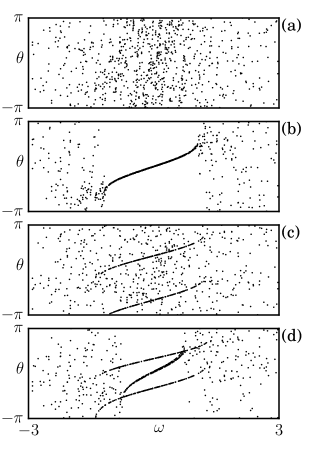
Figure 1: Statistical steady states for the Kuramoto-van Hemmen model. Equation (1) was integrated numerically for $N=1000$ oscillators with Lorentzian distributed frequencies and random initial phases, using a fourth-order Runge-Kutta method with a fixed step size of 0.05. Parameter values: (a) Incoherence: $K_{0}=1,K_{1}=1$; (b) Partial locking: $K_{0}=2.5,K_{1}=1$; (c) Partial antiphase locking: $K_{0}=1,K_{1}=2.75$; (d) Mixed state: $K_{0}=2.5,K_{1}=2.75$. Only oscillators with $-3\leq\omega\leq 3$ are shown.

These four states are not new. They were found and analyzed by Bonilla et al. Bonilla et al. (1993) for a variant of Eq. (1) with a white noise term and a uniform (not Lorentzian) distribution of natural frequencies. The advantage of the present system is that the stability properties and phase boundaries of the four states can be obtained analytically. Figure 2 shows the resulting phase diagram.

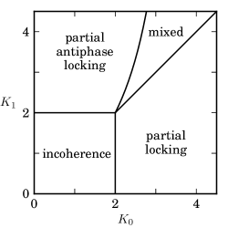
Figure 2: Phase diagram for (1), (2) with $g(\omega)=1/[\pi(1+\omega^{2})]$.

We turn now to the analysis. As mentioned above, the Ott-Antonsen ansatz Ott and Antonsen (2008) has become standard, so we suppress the intermediate steps in the following derivation (but see Ott and Antonsen (2008) for details). The ansatz applies to (1) in the continuum limit and restricts attention to an invariant manifold that determines the system’s long-term dynamics Ott and Antonsen (2009). On this manifold the time-dependent density $\rho(\theta,t,\omega,\xi,\eta)$ of oscillators at phase $\theta$ with natural frequency $\omega$ and van Hemmen parameters $\xi,\eta$ is given by

$$\rho=\frac{1}{2\pi}\left\{1+\left[\sum_{n=1}^{\infty}(\alpha^{*}e^{i\theta})^{n}+{\rm~{}c.c.}\right]\right\}$$ (3)

where $\alpha=\alpha(t,\omega,\xi,\eta)$ and the asterisk and c.c. denote complex conjugation. This density evolves according to

$$\frac{\partial\rho}{\partial t}+\frac{\partial}{\partial\theta}(\rho v) = 0$$ (4)

where $v=v(t,\omega,\xi,\eta)$ denotes the velocity field in the continuum limit,

$$v=\omega+{\rm Im}[e^{-i\theta}(K_{0}Z+K_{1}\xi W_{\eta}+K_{1}\eta W_{\xi})+{\rm~{}c.c.}]$$ (5)

and the complex order parameters $Z$, $W_{\xi}$, and $W_{\eta}$ are

$$Z = \langle e^{i\theta}\rangle,$$

$$W_{\xi} = \langle\xi e^{i\theta}\rangle,$$

$$W_{\eta} = \langle\eta e^{i\theta}\rangle.$$ (6)

The angle brackets $\langle\cdot\rangle$ denote integration with respect to the probability measure $\rho(\theta)d\theta\,g(\omega)d\omega\,p(\xi)d\xi\,p(\eta)d\eta$. The distribution $p$ is normalized so that $\xi$ and $\eta$ equal $\pm 1$ with equal probability $\frac{1}{2}$.

When (3) and (5) are inserted into (4), one finds that the dependence on $\theta$ is satisfied identically if $\alpha(t,\omega,\xi,\eta)$ evolves according to:

$$\dot{\alpha} = -\frac{\alpha^{2}}{2}\left[K_{0}Z^{*}+K_{1}\left(\xi W_{\eta}^{*}+\eta W_{\xi}^{*}\right)\right]+i\omega\alpha$$ (7)

$$+\frac{1}{2}[K_{0}Z+K_{1}(\xi W_{\eta}+\eta W_{\xi})].$$

This system is infinite-dimensional, since there is one equation for each real $\omega$. But its macroscopic dynamics are governed by a much smaller, finite-dimensional set of ODEs. The reduction occurs because the different $\alpha(t,\omega,\xi,\eta)$ in (7) are coupled only through the order parameters $Z$, $W_{\xi}$, and $W_{\eta}$. Those order parameters in turn are expressible, via (6), as integrals involving $\rho$ and therefore $\alpha$ itself. Under the usual analyticity assumptions Ott and Antonsen (2008) on $\alpha$, the various integrals can be expressed in terms of a finite set of $\alpha$’s, and these obey the promised ODEs, as follows.

Consider $Z=\int e^{i\theta}\rho(\theta)d\theta\,g(\omega)d\omega\,p(\xi)d\xi\,p(\eta)d\eta$. To calculate this multiple integral, first substitute (3) for $\rho$ and perform the integration over $\theta$ to get $Z=\int\alpha\,g(\omega)d\omega\,p(\xi)d\xi\,p(\eta)d\eta$. Second, evaluate the integral $\int_{-\infty}^{\infty}\alpha\,g(\omega)d\omega$ by considering $\omega$ as a complex number and computing the resulting contour integral, choosing the contour to be an infinitely large semicircle closed in the upper half plane. The Lorentzian $g(\omega)=1/[\pi(1+\omega^{2})]$ has a simple pole at $\omega=i$, so the residue theorem yields

$$\int_{-\infty}^{\infty}\alpha\,g(\omega)d\omega = \alpha(t,i,\xi,\eta).$$ (8)

Third, integrate over $\xi$ and $\eta$. Since these variables take on the values $\pm 1$ with equal probability, $Z$ receives contributions from four subpopulations: $(\xi,\eta)$=$(+1,+1)$, $(+1,-1)$, $(-1,+1)$, and $(-1,-1)$. If we define the sub-order parameters for these subpopulations as

$$A(t) = \alpha(t,i,+1,+1)$$

$$B(t) = \alpha(t,i,-1,-1)$$

$$C(t) = \alpha(t,i,+1,-1)$$

$$D(t) = \alpha(t,i,-1,+1),$$ (9)

we find that $Z$ is given by

$$Z = \frac{1}{4}(A+B+C+D).$$ (10)

Similar calculations show that the glass order parameters can also be expressed in terms of $A,B,C,D$:

$$W_{\xi} = \dfrac{1}{4}(A-B+C-D),$$

$$W_{\eta} = \dfrac{1}{4}(A-B-C+D).$$ (11)

The sub-order parameters $A,B,C,D$ have physical meanings. For example, $A$ can be thought of as a giant oscillator, a proxy for all the microscopic oscillators with $(\xi,\eta)=(+1,+1)$. Likewise, $B,C$ and $D$ represent giant oscillators for the other subpopulations.

The equations of motion for these giant oscillators are obtained by inserting (10), (11) into (7) and analytically continuing to $\omega=i$. The result is the following closed system:

$$\dot{A} = -\frac{1}{2}A^{2}[K_{0}Z^{*}+\frac{K_{1}}{2}(A^{*}-B^{*})]-A$$

$$+\frac{1}{2}[K_{0}Z+\frac{K_{1}}{2}(A-B)]$$

$$\dot{B} = -\frac{1}{2}B^{2}[K_{0}Z^{*}+\frac{K_{1}}{2}(B^{*}-A^{*})]-B$$

$$+\frac{1}{2}[K_{0}Z+\frac{K_{1}}{2}(B-A)]$$

$$\dot{C} = -\frac{1}{2}C^{2}[K_{0}Z^{*}+\frac{K_{1}}{2}(D^{*}-C^{*})]-C$$

$$+\frac{1}{2}[K_{0}Z+\frac{K_{1}}{2}(D-C)]$$

$$\dot{D} = -\frac{1}{2}D^{2}[K_{0}Z^{*}+\frac{K_{1}}{2}(C^{*}-D^{*})]-D$$ (12)

$$+\frac{1}{2}[K_{0}Z+\frac{K_{1}}{2}(C-D)].$$

Since $A,B,C,$ and $D$ are complex numbers, the system (12) is eight-dimensional.

The four steady states shown in Fig. 1 correspond to four families of fixed points of (12), each of which is characterized by a simple configuration of $A,B,C,D$ in the complex plane. Figure 3 plots those four families schematically on the phase diagram, showing where each exists and is linearly stable. We discuss them in turn.

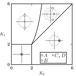
Figure 3: Stable fixed points $A,B,C,D$ for the four states. In each panel, the axes show the region of the complex plane with $-1\leq{\rm~{}Re}(z)\leq 1$ and $-1\leq{\rm~{}Im}(z)\leq 1$. Rotationally equivalent fixed points lie on the dashed circles.

The incoherent state of Fig. 1(a) corresponds to the fixed point at the origin, $A=B=C=D=0$, with order parameters $Z=W_{\xi}=W_{\eta}=0.$ It exists for all $K_{0},\ K_{1}\geq 0$ but is linearly stable iff (if and only if) $K_{0}<2$ and $K_{1}<2$. This stability region is shown as the square in the lower left of Fig. 3.

The partially locked state (Fig. 1(b)) corresponds to a configuration where $A,B,C$ and $D$ all equal the same nonzero complex number, as shown in the lower right panel of Fig. 3. By rotational symmetry, we can assume that $A=B=C=D=R_{PL}>0$. Such a state is a fixed point of (12) iff $K_{0}>2$ and $R_{PL}=\sqrt{1-2/K_{0}}$, in which case it is linearly stable iff $K_{1}<K_{0}$. (There is a trivial zero eigenvalue associated with the rotational symmetry, so what we really mean is that the state is linearly stable to all perturbations other than rotational ones. Likewise, there is a whole circle of partially locked states, all equivalent up to rotation, as indicated by the dashed circle in the lower right panel of Fig. 3.) The order parameters are $Z=\sqrt{1-2/K_{0}}$ and $W_{\xi}=W_{\eta}=0.$

The antiphase state (Fig. 1(c)) corresponds to a fixed point where $A=-B=R_{A}>0$ and $C=D=0$. It exists iff $K_{1}>2$ and $R_{A}=\sqrt{1-2/K_{1}}$. When it exists it is linearly stable iff

$$K_{0}<4K_{1}/(2+K_{1}).$$ (13)

Finally, the mixed state (Fig. 1(d)) corresponds to a configuration where $A=B^{*}$ and $C=D=R_{M}>0$. It exists iff $K_{1}>2$ and $4K_{1}/(2+K_{1})<K_{0}<K_{1}$ (the wedge in the upper right of Fig. 3) and satisfies

$${\rm~{}Re}(A) = \frac{K_{0}}{2K_{1}-K_{0}}\sqrt{1+\frac{2}{K_{1}}-\frac{4}{K_{0}}}$$

$${\rm~{}Im}(A) = 2\sqrt{\frac{(K_{1}-K_{0})(K_{1}(K_{1}-2)+K_{0})}{K_{1}(2K_{1}-K_{0})^{2}}}$$

$$R_{M} = \sqrt{1+\frac{2}{K_{1}}-\frac{4}{K_{0}}}.$$ (14)

We were unable to find the eigenvalues analytically in this final case, but we verified linear stability numerically for a sample of mixed states up to $K_{1}=10^{5}$.

All the transitions in Fig. 3 are continuous (Fig. 4). In particular, the mixed state morphs into the antiphase state on the left side of its stability region, and into the partially locked state on the right side. To verify this, observe that the configuration of $A,B,C,D$ in the mixed state, as parametrized by Eq. (14), continuously deforms into the states on either side of it as $(K_{0},K_{1})$ approaches the relevant stability boundary.

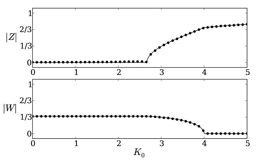
Figure 4: Theory vs. simulation for order parameters. Solid line, exact results; circles, simulations for $N$=$50,000$ oscillators. For $K_{1}$=4, Eq. (1) was integrated using an Euler method with step size 0.01. Each combination of $(\xi,\eta)=(\pm 1,\pm 1)$ was assigned $N/4$ oscillators, with natural frequencies taken from a deterministic Lorentzian distribution: $\omega_{i}$ = $\tan\left[(\pi/2)(2i-n-1)/(n+1)\right]$, for $i=1,\dots,n$ and $n$=$N/4$. The values of the order parameters are shown at $t=200$, by which time convergence to a statistical steady state has occurred.

The glass order parameters $W_{\xi}$ and $W_{\eta}$ are nonzero for the antiphase and mixed states, so in that specific sense the model can be said to exhibit a glassy form of synchronization  Bonilla et al. (1993). Moreover, $W_{\xi}=W_{\eta}$ for all four states, which confirms a conjecture of Bonilla et al. Bonilla et al. (1993). On the other hand, the oscillator model (1), (2) lacks other defining features of a glass, such as a large multiplicity of metastable states and non-exponential relaxation dynamics; the same is true of the original van Hemmen spin-glass model Choy and Sherrington (1984).

Experimental tests of the phase diagram predicted here may be possible in a variety of oscillator systems with programmable coupling. Prime candidates are optical arrays Hagerstrom et al. (2012) or populations of photosensitive chemical oscillators Tinsley et al. (2012) in which the interactions are mediated by a computer-controlled spatial light modulator.

Research supported in part by an NSF Graduate Research Fellowship to I.M.K and NSF Award 1006272 to I.M.L. We thank Murray Strogatz for helpful discussions.

References

- Winfree (1967) A. T. Winfree, J. Theor. Biol. 16, 15 (1967).
- Kuramoto (1984) Y. Kuramoto, Chemical Oscillations, Waves, and Turbulence (Springer, Berlin, 1984).
- Acebrón et al. (2005) J. A. Acebrón, L. L. Bonilla, C. J. Pérez Vicente, F. Ritort, and R. Spigler, Rev. Mod. Phys. 77, 137 (2005).
- Strogatz (2000) S. H. Strogatz, Physica D 143, 1 (2000).
- Pikovsky et al. (2003) A. Pikovsky, M. Rosenblum, and J. Kurths, Synchronization (Cambridge University Press, 2003).
- Strogatz (2003) S. H. Strogatz, Sync (Hyperion, 2003).
- Daido (1987) H. Daido, Prog. Theor. Phys. 77, 622 (1987).
- Binder and Young (1986) K. Binder and A. P. Young, Rev. Mod. Phys. 58, 801 (1986).
- Daido (1992) H. Daido, Phys. Rev. Lett. 68, 1073 (1992).
- Sherrington and Kirkpatrick (1975) D. Sherrington and S. Kirkpatrick, Phys. Rev. Lett. 35, 1792 (1975).
- Stiller and Radons (1998) J. C. Stiller and G. Radons, Phys. Rev. E 58, 1789 (1998).
- Daido (2000) H. Daido, Phys. Rev. E 61, 2145 (2000).
- Stiller and Radons (2000) J. C. Stiller and G. Radons, Phys. Rev. E 61, 2148 (2000).
- Bonilla et al. (1993) L. Bonilla, C. P. Vicente, and J. Rubi, Journal of Statistical Physics 70, 921 (1993).
- Paissan and Zanette (2008) G. H. Paissan and D. H. Zanette, Physica D 237, 818 (2008).
- Iatsenko et al. (2013) D. Iatsenko, P. V. McClintock, and A. Stefanovska, arXiv preprint arXiv:1303.4453 (2013).
- Hong and Strogatz (2011) H. Hong and S. H. Strogatz, Phys. Rev. Lett. 106, 054102 (2011).
- van Hemmen (1982) J. L. van Hemmen, Phys. Rev. Lett. 49, 409 (1982).
- Ott and Antonsen (2008) E. Ott and T. M. Antonsen, Chaos 18, 037113 (2008).
- Childs and Strogatz (2008) L. M. Childs and S. H. Strogatz, Chaos 18, 043128 (2008).
- Pikovsky and Rosenblum (2008) A. Pikovsky and M. Rosenblum, Phys. Rev. Lett. 101, 264103 (2008).
- Ott and Antonsen (2009) E. Ott and T. M. Antonsen, Chaos 19, 023117 (2009).
- Martens et al. (2009) E. A. Martens, E. Barreto, S. H. Strogatz, E. Ott, P. So, and T. M. Antonsen, Phys. Rev. E 79, 026204 (2009).
- Laing (2009) C. R. Laing, Physica D 238, 1569 (2009).
- Komarov and Pikovsky (2011) M. Komarov and A. Pikovsky, Phys. Rev. E 84, 016210 (2011).
- Montbrió and Pazó (2011) E. Montbrió and D. Pazó, Phys. Rev. E 84, 046206 (2011).
- Iatsenko et al. (2013) D. Iatsenko, S. Petkoski, P. V. E. McClintock, and A. Stefanovska, Phys. Rev. Lett. 110, 064101 (2013).
- Choy and Sherrington (1984) T. Choy and D. Sherrington, Journal of Physics C: Solid State Physics 17, 739 (1984).
- Hagerstrom et al. (2012) A. M. Hagerstrom, T. E. Murphy, R. Roy, P. Hövel, I. Omelchenko, and E. Schöll, Nature Physics 8, 658 (2012).
- Tinsley et al. (2012) M. R. Tinsley, S. Nkomo, and K. Showalter, Nature Physics 8, 662 (2012).