Synthetic light curves and spectra for three-dimensional delayed-detonation models of Type Ia supernovae

Abstract

In a companion paper, Seitenzahl et al. (2013) have presented a set of three-dimensional delayed detonation models for thermonuclear explosions of near-Chandrasekhar mass white dwarfs (WDs). Here, we present multi-dimensional radiative transfer simulations that provide synthetic light curves and spectra for those models. The model sequence explores both changes in the strength of the deflagration phase (which is controlled by the ignition configuration in our models) and the WD central density. In agreement with previous studies, we find that the strength of the deflagration significantly affects the explosion and the observables. Variations in the central density also have an influence on both brightness and colour, but overall it is a secondary parameter in our set of models. In many respects, the models yield a good match to the observed properties of normal Type Ia supernovae (SNe Ia): peak brightness, rise/decline time scales and synthetic spectra are all in reasonable agreement. There are, however, several differences. In particular, the models are systematically too red around maximum light, manifest spectral line velocities that are a little too high and yield $I$-band light curves that do not match observations. Although some of these discrepancies may simply relate to approximations made in the modelling, some pose real challenges to the models. If viewed as a complete sequence, our models do not reproduce the observed light-curve width-luminosity relation (WLR) of SNe Ia: all our models show rather similar $B$-band decline rates, irrespective of peak brightness. This suggests that simple variations in the strength of the deflagration phase in Chandrasekhar-mass deflagration-to-detonation models do not readily explain the observed diversity of normal SNe Ia. This may imply that some other parameter within the Chandrasekhar-mass paradigm is key to the WLR, or that a substantial fraction of normal SNe Ia arise from an alternative explosion scenario.

1 Introduction

It is generally accepted that Type Ia supernovae (SNe Ia) are the result of the thermonuclear explosion of carbon-oxygen (CO) white dwarf (WD) stars (see e.g.  Hillebrandt & Niemeyer, 2000; Hillebrandt et al., 2013). However, the evolutionary channel leading to explosion and the mechanisms by which the thermonuclear flame ignites and propagates remain unclear. The best known and most widely studied explosion model for SNe Ia is the single-degenerate Chandrasekhar-mass scenario. In that model, a CO WD gains mass by accretion from a non-degenerate companion star. When the WD mass draws near to the Chandrasekhar limit, carbon burning ignites near to the centre of the WD. Although initially neutrino cooling is sufficient to prevent explosion, heat released by carbon burning eventually gives rise to local conditions where a thermonuclear runaway can occur, leading to the birth of a thermonuclear deflagration flame.

Three-dimensional (3D) explosion simulations of pure deflagration models for SNe Ia have been considered in several studies (e.g.  Reinecke et al., 2002; Gamezo et al., 2003; Röpke & Hillebrandt, 2005; Röpke & Bruckschen, 2008). Although it is possible for deflagration models to yield explosions in which the WD is entirely disrupted, such models struggle to produce a sufficiently large mass of ⁵⁶Ni to account for the observed brightness of normal SNe Ia: even with favourably chosen initial conditions, only around ${\sim}0.33$ M_⊙ of ⁵⁶Ni are produced (Röpke et al. 2007; see also Ma et al. 2013). Deflagration models are therefore most promising for explaining certain sub-luminous SNe Ia. We also note that, depending on the ignition configuration, deflagration simulations can give rise to explosions in which only a part of the mass of the WD is ejected (Jordan et al., 2012) – this scenario gives a good match to the observed properties of the faint/spectroscopically peculiar class of 2002cx-like SNe Ia (Kromer et al., 2013).

To account for the brightness of normal SNe Ia, more ⁵⁶Ni must be synthesised than is expected from pure deflagration models. For near-Chandrasekhar mass models, this can be achieved by invoking a thermonuclear detonation at some point during or after the propagation of the deflagration flame. A few such “delayed detonation” mechanisms have been proposed, including spontaneous deflagration-to-detonation transition (DDT) models (Khokhlov, 1991), the gravitationally confined detonation model (Plewa et al., 2004), the pulsational detonation model (e.g.  Khokhlov et al., 1992; Bravo & García-Senz, 2009; Bravo et al., 2009) and the pulsationally assisted gravitationally confined detonation model (Jordan et al., 2012). In this study, we will focus on DDT models, in which it is argued that the deflagration flame transitions into a detonation during the late stages of the explosion. This may occur when, due to the low fuel densities, the flame structure broadens and turbulence starts to affect the microphysical processes. If in this “distributed burning regime” turbulent velocity fluctuations are strong enough to mix fuel and ashes efficiently, a detonation may ignite via the Zel’dovich gradient mechanism (e.g., Woosley, 2007; Woosley et al., 2009).

Synthetic spectra and light curves have been presented for sets of near-Chandrasekhar mass DDT models in several previous studies. One-dimensional (1D) DDT models have been studied by e.g. Höflich et al. (1995), Höflich & Khokhlov (1996) and Blondin et al. (2013), while 2D simulations were presented by Kasen et al. (2009) and Blondin et al. (2011). Dimensionality, however, is an important consideration for DDT models. Since the propagation of the deflagration flame is controlled by turbulence and the hot deflagration ash is subject to buoyancy (and secondary) instabilities, full 3D simulations are needed both to model the flame propagation and predict the final composition of the ejecta. Recently, Seitenzahl et al. (2013) presented a set of fourteen 3D DDT explosion simulations (and associated nucleosynthesis post-processing) for SNe Ia. These models differ from each other in the adopted ignition configuration of the deflagration flame and in the central density of the WD. Therefore, they provide a useful set of models with which to consider whether fully 3D DDT models can account for the observed properties of normal SNe Ia and to investigate how observable quantities are affected by key initial conditions of explosion simulations. To this end, in this paper we present the results of radiative transfer calculations for the Seitenzahl et al. (2013) models and compare them with observed properties of SNe Ia.

In Section 2 we remind the reader of salient details of the Seitenzahl et al. (2013) models and describe our radiative transfer calculations. We present results of our calculations in Section 3. Implications of our work are discussed in Section 4 and conclusions are summarised in Section 5.

2 Simulations

2.1 Explosion models

Below we will present the results of radiative transfer calculations applied to the set of fourteen explosion models described by Seitenzahl et al. (2013). The hydrodynamics simulations were carried out using leafs, which is a 3D finite-volume code that uses a levelset method to track thermonuclear flame fronts (see Seitenzahl et al., 2013, and references therein). As initial conditions for the explosion simulation, Seitenzahl et al. (2013) adopted a cold hydrostatic WD with uniform composition: ¹²C/¹⁶O/²²Ne of 47.5/50/2.5 per cent by mass. In a future study, we plan to investigate the consequences of adopting more realistic, non-uniform initial compositions, but for all models in this paper, the WD composition is homogeneous.

The explosions are ignited by inserting a distribution of deflagration sparks: small spherical ($10^{6}$ cm radius) regions where it is assumed that a local thermonuclear runaway has given birth to a deflagration. It is well established from multi-dimensional simulations that the ignition configuration can significantly affect the outcome of DDT models (Golombek & Niemeyer, 2005; Röpke et al., 2007; Mazzali et al., 2007; Bravo & García-Senz, 2008; Kasen et al., 2009; Krueger et al., 2012; Seitenzahl et al., 2013). In our models, a larger number of sparks means that the total surface area of the deflagration is initially bigger, leading to more rapid fuel consumption. Also, more sparks lead to higher order spatial modes being excited in the structure of the flame front, affecting the growth of instabilities and the development of turbulence. It follows that models ignited with large numbers of sparks have stronger deflagration phases. We stress that the number of ignition sparks in any given model should not be interpreted literally: the numbers of sparks used in this study were chosen, by trial and error, in order to produce models with a sufficiently wide range of ⁵⁶Ni masses to encompass the bulk of normal SNe Ia. Thus, the models are not motivated by consideration of ignition conditions and do not address the question of whether deflagrations of the corresponding strength would be realised in Nature. Instead, the purpose of these models is twofold. First, to investigate whether a good match to observed SNe Ia can be found for some choice of the deflagration strength. Second, to explore the hypothesis that simple variations in the deflagration strength in DDT models might explain the observed diversity of SNe Ia. In this context, the number / location of sparks is merely a convenient parametrization that allows us to realise a set of models with a wide range of rates of fuel consumption during the deflagration phase.

Twelve of the fourteen models form a sequence along which the models differ only in the number (and location) of the ignition sparks adopted for the deflagration flame. In these models, the number of ignition sparks varies from 1 to 1600: throughout this paper we will refer to the individual models by their number of ignition sparks as Nx (x ranging from 1 to 1600). The ignition sparks are placed fairly close to the centre of the WD ($r<2.5\times 10^{7}$ cm). In two of the models the sparks are particularly centrally concentrated: these two models are identified by NxC. For details of the ignition geometries and the algorithm used to place the sparks, see Seitenzahl et al. (2013). In each of these twelve models, the WD central density was chosen to be $2.9\times 10^{9}$ g cm^-3 (which gives a total WD mass of $1.400$ $\mathrm{M}_{\odot}$).

The remaining two models differ from the other twelve in the choice of WD central density. In one case a low central density of $1\times 10^{9}$ g cm^-3 ($1.361$ $\mathrm{M}_{\odot}$) is adopted, while in the other a high value of $5.5\times 10^{9}$ g cm^-3 ($1.416$ $\mathrm{M}_{\odot}$) is used. The WD central density has been suggested as a potential secondary parameter that can affect the outcome of a DDT explosion, primarily via its influence on the masses of both ⁵⁶Ni and stable iron-group elements that are synthesised during nuclear burning at high density (Krueger et al., 2010; Seitenzahl et al., 2011; Krueger et al., 2012; Seitenzahl et al., 2013). To facilitate direct comparison, the ignition geometries for our two models with different central densities were chosen to be the same as for the N100 model. We will therefore refer to the models with high and low central densities as N100H and N100L, respectively.

Table 1: Asymptotic ejecta kinetic energies, ⁵⁶Ni masses, light-curve rise and decline parameters, peak absolute optical magnitudes and colours for our simulations. For each quantity, the value derived from the angle-averaged light curve is quoted along with the range obtained from our full set of orientation-dependent light curves (specified as a $\pm$ range on each derived value).

Model	$E_{\rm kin}$	$M(^{56}$Ni$)$	$t_{\rm max}^{\rm bol}$	$t_{\rm max}^{B}$	$M^{\rm bol}_{\rm max}$	$U_{\rm max}$	$B_{\rm max}$	$V_{\rm max}$	$R_{\rm max}$	$I_{\rm max}$
	$10^{51}$ erg	M⊙	daysa	days	maga	mag	mag	mag	mag	mag
N1	$1.67$	$1.10$	$16.6_{-0.4}^{+0.4}$	$16.5_{-0.6}^{+0.4}$	$-19.48^{-0.06}_{+0.06}$	$-20.39^{-0.13}_{+0.17}$	$-19.93^{-0.06}_{+0.05}$	$-20.12^{-0.03}_{+0.02}$	$-19.56^{-0.05}_{+0.04}$	$-19.70^{-0.05}_{+0.05}$
N3	$1.61$	$1.03$	$17.7_{-0.6}^{+1.2}$	$17.4_{-0.7}^{+0.6}$	$-19.40^{-0.21}_{+0.40}$	$-20.18^{-0.40}_{+1.19}$	$-19.80^{-0.22}_{+0.57}$	$-20.08^{-0.11}_{+0.13}$	$-19.59^{-0.09}_{+0.06}$	$-19.63^{-0.13}_{+0.14}$
N5	$1.59$	$0.97$	$18.0_{-0.7}^{+0.9}$	$17.7_{-0.7}^{+0.9}$	$-19.33^{-0.16}_{+0.21}$	$-20.05^{-0.31}_{+0.50}$	$-19.71^{-0.18}_{+0.31}$	$-20.00^{-0.09}_{+0.09}$	$-19.60^{-0.08}_{+0.06}$	$-19.60^{-0.10}_{+0.09}$
N10	$1.60$	$0.93$	$18.1_{-0.7}^{+0.7}$	$17.7_{-0.5}^{+0.5}$	$-19.29^{-0.17}_{+0.11}$	$-19.94^{-0.30}_{+0.25}$	$-19.66^{-0.16}_{+0.14}$	$-19.96^{-0.10}_{+0.06}$	$-19.60^{-0.12}_{+0.07}$	$-19.59^{-0.11}_{+0.06}$
N20	$1.52$	$0.77$	$18.3_{-1.1}^{+1.2}$	$17.7_{-1.0}^{+1.0}$	$-19.09^{-0.13}_{+0.07}$	$-19.55^{-0.26}_{+0.15}$	$-19.34^{-0.15}_{+0.16}$	$-19.73^{-0.07}_{+0.06}$	$-19.55^{-0.09}_{+0.06}$	$-19.51^{-0.11}_{+0.08}$
N100H	$1.53$	$0.69$	$18.2_{-0.9}^{+1.0}$	$16.8_{-1.1}^{+1.0}$	$-18.96^{-0.09}_{+0.08}$	$-19.08^{-0.23}_{+0.22}$	$-19.10^{-0.18}_{+0.14}$	$-19.65^{-0.08}_{+0.07}$	$-19.57^{-0.04}_{+0.04}$	$-19.53^{-0.05}_{+0.08}$
N40	$1.47$	$0.65$	$18.3_{-1.1}^{+0.7}$	$17.3_{-1.0}^{+0.7}$	$-18.93^{-0.07}_{+0.09}$	$-19.14^{-0.28}_{+0.33}$	$-19.11^{-0.12}_{+0.16}$	$-19.57^{-0.05}_{+0.07}$	$-19.50^{-0.03}_{+0.03}$	$-19.46^{-0.08}_{+0.06}$
N100	$1.46$	$0.60$	$18.2_{-0.7}^{+0.8}$	$17.0_{-0.7}^{+0.7}$	$-18.87^{-0.07}_{+0.05}$	$-18.98^{-0.19}_{+0.22}$	$-19.02^{-0.10}_{+0.07}$	$-19.51^{-0.05}_{+0.06}$	$-19.47^{-0.03}_{+0.03}$	$-19.44^{-0.04}_{+0.04}$
N150	$1.41$	$0.56$	$18.0_{-0.6}^{+0.9}$	$16.5_{-0.9}^{+1.0}$	$-18.80^{-0.05}_{+0.08}$	$-18.94^{-0.14}_{+0.18}$	$-18.82^{-0.10}_{+0.13}$	$-19.39^{-0.05}_{+0.05}$	$-19.43^{-0.03}_{+0.04}$	$-19.43^{-0.04}_{+0.05}$
N100L	$1.37$	$0.53$	$18.2_{-1.1}^{+0.9}$	$17.2_{-1.0}^{+0.8}$	$-18.76^{-0.09}_{+0.12}$	$-18.89^{-0.30}_{+0.37}$	$-18.89^{-0.16}_{+0.22}$	$-19.34^{-0.09}_{+0.10}$	$-19.34^{-0.05}_{+0.04}$	$-19.29^{-0.06}_{+0.07}$
N300C	$1.42$	$0.51$	$17.4_{-0.8}^{+0.7}$	$16.0_{-1.4}^{+0.8}$	$-18.76^{-0.04}_{+0.06}$	$-18.70^{-0.13}_{+0.14}$	$-18.69^{-0.11}_{+0.17}$	$-19.29^{-0.06}_{+0.08}$	$-19.38^{-0.04}_{+0.05}$	$-19.41^{-0.06}_{+0.06}$
N200	$1.34$	$0.41$	$18.1_{-1.3}^{+0.9}$	$16.1_{-2.0}^{+1.2}$	$-18.53^{-0.07}_{+0.11}$	$-18.46^{-0.18}_{+0.25}$	$-18.46^{-0.12}_{+0.20}$	$-19.06^{-0.06}_{+0.13}$	$-19.20^{-0.06}_{+0.10}$	$-19.28^{-0.06}_{+0.05}$
N1600	$1.32$	$0.36$	$18.4_{-0.8}^{+1.0}$	$16.0_{-1.1}^{+1.4}$	$-18.39^{-0.07}_{+0.09}$	$-18.10^{-0.26}_{+0.30}$	$-18.26^{-0.14}_{+0.21}$	$-18.93^{-0.06}_{+0.10}$	$-19.10^{-0.05}_{+0.09}$	$-19.18^{-0.05}_{+0.04}$
N1600C	$1.20$	$0.32$	$18.5_{-0.7}^{+0.6}$	$16.0_{-0.7}^{+0.6}$	$-18.26^{-0.06}_{+0.08}$	$-18.13^{-0.36}_{+0.29}$	$-18.16^{-0.11}_{+0.14}$	$-18.73^{-0.06}_{+0.07}$	$-18.94^{-0.03}_{+0.05}$	$-19.06^{-0.06}_{+0.05}$

Model	$B-V$	$V-R$	$V-I$	$\Delta m_{15}^{B}$	$\Delta m_{15}^{V}$
	magb	magb	magb	mag	mag
N1	$0.15_{-0.04}^{+0.06}$	$-0.53_{-0.05}^{+0.04}$	$-1.24_{-0.05}^{+0.05}$	$1.36_{-0.11}^{+0.11}$	$0.70_{-0.05}^{+0.04}$
N3	$0.23_{-0.12}^{+0.44}$	$-0.45_{-0.07}^{+0.10}$	$-1.11_{-0.13}^{+0.15}$	$1.27_{-0.36}^{+0.20}$	$0.74_{-0.08}^{+0.08}$
N5	$0.23_{-0.10}^{+0.25}$	$-0.36_{-0.07}^{+0.06}$	$-0.93_{-0.08}^{+0.09}$	$1.34_{-0.25}^{+0.13}$	$0.77_{-0.08}^{+0.11}$
N10	$0.24_{-0.07}^{+0.08}$	$-0.31_{-0.04}^{+0.04}$	$-0.82_{-0.08}^{+0.09}$	$1.37_{-0.13}^{+0.10}$	$0.79_{-0.06}^{+0.10}$
N20	$0.31_{-0.10}^{+0.11}$	$-0.13_{-0.06}^{+0.08}$	$-0.40_{-0.12}^{+0.12}$	$1.34_{-0.17}^{+0.09}$	$0.83_{-0.11}^{+0.05}$
N100H	$0.43_{-0.11}^{+0.09}$	$-0.03_{-0.05}^{+0.05}$	$-0.20_{-0.08}^{+0.10}$	$1.33_{-0.12}^{+0.13}$	$0.86_{-0.06}^{+0.08}$
N40	$0.35_{-0.07}^{+0.10}$	$-0.02_{-0.05}^{+0.05}$	$-0.16_{-0.10}^{+0.08}$	$1.36_{-0.08}^{+0.08}$	$0.87_{-0.08}^{+0.04}$
N100	$0.37_{-0.07}^{+0.07}$	$0.02_{-0.04}^{+0.04}$	$-0.09_{-0.08}^{+0.07}$	$1.39_{-0.08}^{+0.09}$	$0.88_{-0.09}^{+0.06}$
N150	$0.48_{-0.07}^{+0.07}$	$0.07_{-0.04}^{+0.05}$	$0.02_{-0.05}^{+0.06}$	$1.30_{-0.13}^{+0.10}$	$0.85_{-0.10}^{+0.06}$
N100L	$0.35_{-0.11}^{+0.11}$	$0.05_{-0.05}^{+0.07}$	$-0.03_{-0.12}^{+0.08}$	$1.34_{-0.16}^{+0.12}$	$0.85_{-0.11}^{+0.09}$
N300C	$0.49_{-0.09}^{+0.08}$	$0.11_{-0.04}^{+0.06}$	$0.11_{-0.06}^{+0.10}$	$1.29_{-0.22}^{+0.11}$	$0.86_{-0.11}^{+0.10}$
N200	$0.50_{-0.06}^{+0.07}$	$0.15_{-0.03}^{+0.05}$	$0.19_{-0.09}^{+0.11}$	$1.26_{-0.27}^{+0.14}$	$0.88_{-0.14}^{+0.07}$
N1600	$0.56_{-0.11}^{+0.12}$	$0.19_{-0.04}^{+0.04}$	$0.24_{-0.07}^{+0.10}$	$1.16_{-0.19}^{+0.14}$	$0.88_{-0.08}^{+0.08}$
N1600C	$0.46_{-0.07}^{+0.07}$	$0.20_{-0.04}^{+0.04}$	$0.28_{-0.06}^{+0.07}$	$1.17_{-0.14}^{+0.13}$	$0.79_{-0.08}^{+0.10}$

^a The rise time $t_{\rm max}^{\rm bol}$ and peak absolute magnitude $M^{\rm bol}_{\rm max}$ are derived from our $UBVRIJHK$ bolometric light curves.
^b Colours are given at the epoch of $B$-band maximum light.

For all the simulations in this study, the same DDT criterion was used, based on the strength of turbulent velocity fluctuations at the flame front (see Seitenzahl et al. 2013 and Ciaraldi-Schoolmann et al. 2013 for details). In all models at least one detonation occurred and the WD was always completely disrupted by the release of thermonuclear energy. By design (see above), the model sequence explores a sufficiently wide range of deflagration strengths that the range of ⁵⁶Ni masses predicted by the simulations is large (0.32 – 1.1 M_⊙). The ⁵⁶Ni mass is generally anti-correlated with the number of ignition sparks adopted (i.e., a larger number of ignition sparks leads to a stronger deflagration phase and more expansion of the WD before detonation occurs). Table 1 lists the models in order of synthesised ⁵⁶Ni mass and gives both the total ⁵⁶Ni mass and the asymptotic explosion energy ($E_{\rm kin}$) in each case.

The leafs simulations were run until $t=100$ s after ignition, by which point the dynamics of the ejecta were very close to free expansion. Seitenzahl et al. (2013) carried out post-processing nucleosynthesis calculations (384-isotope network) to obtain detailed nucleosynthesis yields for each model. Those calculations were performed using the thermodynamic trajectories of $10^{6}$ passive Lagrangian tracer particles that were recorded during the hydrodynamics simulations (following Travaglio et al., 2004; Seitenzahl et al., 2010). We have used the final positions (and compositions) of the tracer particles to reconstruct the full 3D composition of the ejecta via a smoothed-particle-hydrodynamics-like algorithm (as described by Kromer et al., 2010).

2.2 Radiative transfer simulations

For each model, we use the artis code (Sim, 2007; Kromer & Sim, 2009) to compute synthetic light curves and spectra. artis employs a Monte Carlo (MC) algorithm (Lucy, 2002, 2003, 2005) to carry out multi-dimensional, time-dependent radiative transfer calculations for homologously expanding SN ejecta.

As input to artis, we take the density and composition structure obtained from the final state of the explosion simulations (Section 2.1), remapped to a uniform 3D Cartesian grid of $50^{3}$ cells. For all times after $t=100$ s (the end of the leafs simulations), the ejecta dynamics are assumed to be well-described by an homologous expansion law. The artis calculations were started at $t=2$ days after explosion. As described by Lucy (2005), energy generated by radioactive decays before $t=2$ days is included by assuming that it has been trapped and advected with the homologously expanding ejecta up to the start of the MC simulation. The radiative transfer simulations are run until $120$ days after explosion in a sequence of 111 logarithmically spaced time steps. For each simulation a total of $1.024\times 10^{8}$ MC quanta were used. Angle-averaged spectra and light curves were obtained by appropriate binning of emergent MC quanta as functions of photon frequency and escape time. In addition, for each model, orientation-dependent synthetic observables were obtained by further binning of the quanta in 100 orientation bins (each of equal solid angle).

All radiative transfer calculations were performed using our atomic data set drawn from Kurucz & Bell (1995) (see Kromer & Sim, 2009), expanded to included ions i – vii for $20<Z<29$, as in Sim et al. (2012). We note, based on the comparisons in Kromer & Sim (2009), that the Kurucz & Bell (1995) line list yields optical spectra that agree well with more expensive calculations involving an even larger atomic data set, making it adequate for this study (which will focus on optical comparisons). We note, however, that the near-infrared (NIR) region is more sensitive to the choice of atomic data [Kromer & Sim (2009) found that using an extended set of atomic data for the iron-group elements led to an increase in the early time NIR light curves by several tenths of a magnitude, compared to our standard Kurucz & Bell line list; see also Kasen (2006)]. This must be borne in mind when comparing our synthetic NIR light curves to observations.

3 Results

3.1 Synthetic light curves

In this section, we will focus on presenting the synthetic light curves and colours of our models, deferring discussion of spectral features to the next section.

3.1.1 Angle-averaged light curves

Bolometric ($UBVRIJHK$) and $B$-band rise times ($t_{\rm max}^{\rm bol}$ and $t_{\rm max}^{B}$, respectively), peak absolute magnitudes, optical colours at $t_{\rm max}^{B}$ and values of the decline rate parameters $\Delta m_{15}^{B}$ and $\Delta m_{15}^{V}$ derived from our angle-averaged light curves are tabulated in Table 1. Complete synthetic angle-averaged bolometric ($UBVRIJHK$) and photometric band-limited light curves are shown for subsets of our models in Figures 1 and 2.

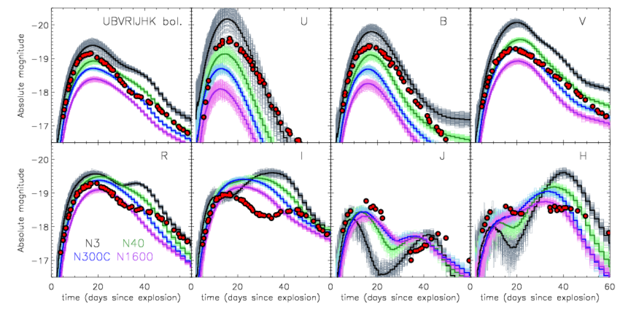
Figure 1: Angle-averaged light curves ($UBVRIJHK$ bolometric, $U$-, $B$-, $V$-, $R$-, $I$-, $J$-, and $H$-bands) for four of our explosion models with differing deflagration strengths (heavy-drawn lines). To indicate the degree of sensitivity to orientation, the corresponding bands of lightly drawn lines shown the light curves from each of our 100 viewing angle bins. Note that Monte Carlo noise affects the angle-dependent light curves, particularly in bands/at epochs when the flux is relatively small (e.g. the $H$-band at early times). In each panel we show observations of SN 2005cf (filled circles) from Pastorello et al. (2007). For ease of comparison, the observed light curves are plotted assuming a $B$-band rise time of 17 days and are corrected for reddening (using parameters from Pastorello et al. 2007).

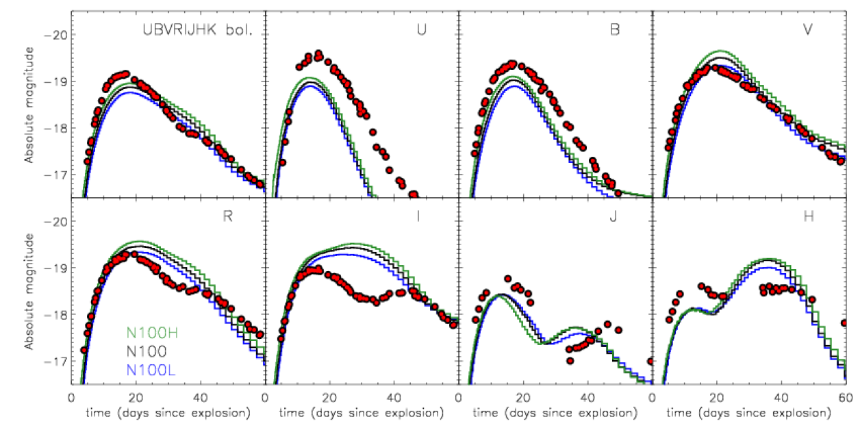
Figure 2: As Figure 1, but showing our explosion models with differing WD central densities. For clarity, angle-dependent light curves are omitted here.

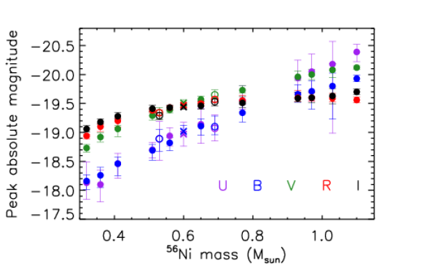
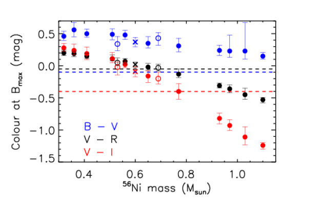
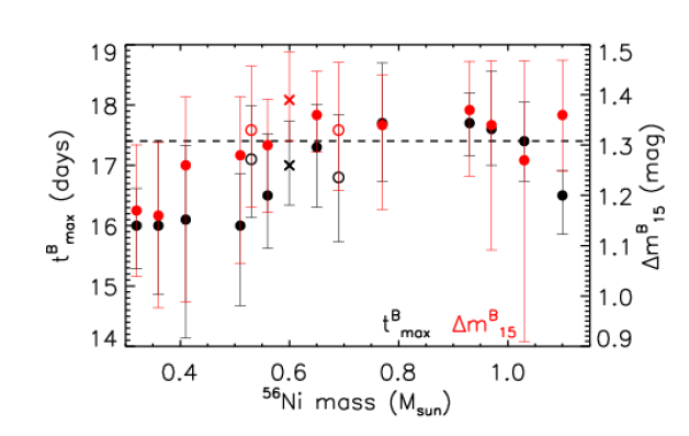
Figure 3: Light curve properties of the models versus ⁵⁶Ni mass. Filled circles show angle-averaged results from our sequence of models that differ only in the choice of ignition properties (which parametrizes the deflagration strength). Open circles show our models with differing WD central densities. Crosses indicate model N100 (which can be considered a part of both sequences of models). The vertical bars indicate the spread due to observer orientation. Top panel: Peak absolute magnitudes in optical bands ($U$, $B$, $V$, $R$ and $I$). Middle panel: Colours at $t_{\rm max}^{B}$. The dashed lines indicate the typical observed peak colours for normal SNe Ia (Blondin et al. 2011). Bottom panel: $B$-band light curve time scales (rise time to peak, $t_{\rm max}^{B}$ and decline rate parameter $\Delta m_{15}^{B}$). The dashed line indicates the mean value of $t_{\rm max}^{B}$ derived from observations by (Strovink, 2007).

As expected based on the ⁵⁶Ni masses (0.32 – 1.1 M_⊙, Seitenzahl et al., 2013), the models predict a wide range of brightnesses in the optical bands (Table 1, Figure 1), sufficient to encompass the range of spectroscopically normal SNe Ia. In the models, this diversity is driven by the choice of the number and location of ignition sparks (which controls the strength of the deflagration phase): compared to the variations between models with different ignition conditions, the effect of varying the WD central density is relatively modest (Figure 2).

The peak brightness variation between models is largest in the bluest bands (see top panel of Figure 3): the models span a range in $U_{\rm max}$ of ${\,\hbox{\lower 2.58334pt\hbox{$\sim$}\hbox to0.0pt{\hss\raise 2.58334pt\hbox{$>$}}}\,}2.5$ mag compared to only ${\sim}0.7$ mag in $I_{\rm max}$. Among models with the same WD central density, angle-averaged $U_{\rm max}$, $B_{\rm max}$ and $V_{\rm max}$ show nearly monotonic decrease (i.e. brightening) with increasing ⁵⁶Ni mass. The trend in $R_{\rm max}$ and $I_{\rm max}$ is weaker and eventually turns over at the largest ⁵⁶Ni masses. Our models with higher and lower central density are slightly displaced from the trends shown by the other models, but only by a few tenths of a magnitude.

The differing trends between photometric bands along our model sequence mean that the SN colours also vary. This is illustrated for $B-V$, $V-R$ and $V-I$ at $t_{\rm max}^{B}$ in the middle panel of Figure 3. Each of these peak colours shows a “brighter-bluer” trend along our model sequence. $B-V$ varies relatively little (and is always positive) but $V-I$ is more than 1 mag bluer in our brightest models than in our faintest. As for the peak magnitudes in the blue bands, the colour changes roughly monotonically with the ⁵⁶Ni mass among the models with the same WD central density.

For all the models, maximum light (in angle-averaged $B$-band) occurs between 16 and 18 days after explosion, roughly consistent with observations (Strovink, 2007; Hayden et al., 2010; Ganeshalingam et al., 2011). There is some systematic variation of $t_{\rm max}^{B}$ along our model sequence (see last panel of Figure 3), but it is not very strong. The post-maximum light curve decline parameter ($\Delta m_{15}^{B}$) is also rather similar in all the models, typically around 1.3 mag.

Comparison of our angle-averaged light curves to photometric observations of normal SNe Ia clearly favours the models with intermediate deflagration strengths: N100H, N40, N100, N150, N100L and N300C. In the $B$, $V$ and $R$ optical bands these models provide reasonable matches to the light curves of normal SNe Ia (e.g. SN 2005cf [Pastorello et al. 2007], shown in Figures 1 and 2). There are some significant shortcomings, however. In particular, for all the models, there is a systematic discrepancy in synthetic optical colours: the models are too red. For example, normal SNe Ia at peak typically have $B-V$ in the range $-0.2$ to $0.0$ (see e.g., Blondin et al., 2011), while all our models have peak $B-V>0$ at $t_{\rm max}^{B}$ (see Figure 3 and Figure 4). The redness problem is most severe for models with strong deflagrations ($\,\hbox{\lower 2.58334pt\hbox{$\sim$}\hbox to0.0pt{\hss\raise 2.58334pt\hbox{$>$}}}\,200$ ignition sparks) but it persists throughout the sequence, appearing as a clear offset in the relation between $B_{\rm max}$ and $V_{\rm max}$ as compared to observations (see Figure 4). We attribute the red colours to excessive line blocking in the blue, primarily by iron-group elements. Of particular importance in the current models is the location of the deflagration burning products. In 1D models (e.g. the W7 model of Nomoto et al. 1984 or the models of Höflich et al. 1995, Höflich & Khokhlov 1996 and Blondin et al. 2013), the products of highest density burning (e.g. stable iron-group material) are centrally concentrated but for models involving a deflagration this is an artificial consequence of the imposed spherical symmetry. Instead, owing to buoyancy, in our multi-dimensional simulations the deflagration ash is not confined to a low-velocity quasi-spherical core but rather forms a clumpy shell-like structure at intermediate velocities. This material is exterior to most of the ⁵⁶Ni-rich regions and immediately interior to (or even mixed through) the Si/S-rich regions in many of the models (see figures 3 and 4 of Seitenzahl et al. 2013). As such, it is able to significantly affect the spectrum in the photospheric phase around and after maximum light.

Our optical light curves tend to decline slightly more quickly post-maximum than do the bulk of normal SNe Ia (the models typically have $\Delta m_{15}^{B}\sim 1.3$ and $\Delta m_{15}^{V}\sim 0.8$; see Figure 5). More importantly, viewed as a sequence, the models fail to show clear width-luminosity relations (WLRs) in the optical bands, in contrast to observations (see Figure 5). This suggests that the variation amongst our current models does not provide a good description of the differences between real events in the main SNe Ia population, a key conclusion to which we will return in Section 4.

In the $I$-band the model light curves provide a rather poor match to observations, typically remaining too bright for too long. Accurate modelling of the $I$-band can be strongly affected by the Ca ii infrared triplet features. This becomes a prominent emission feature in the models post maximum light, the strength of which is likely overestimated since artis does not currently account for forbidden line emission in iron-group elements. Consequently, the poor match in the $I$-band may be partially attributed to shortcomings in the radiative transfer calculations. We note, however, that better agreement was found using the same numerical codes for models of sub-Chandrasekhar mass explosions (Sim et al., 2010) and merger models (Pakmor et al., 2012) – thus the $I$-band excess in the models may also point to a genuine shortcoming of the models.

In the NIR bands, the models with $>20$ ignition sparks qualitatively agree with observations: the NIR light curves generally show double peaks and the model-to-model variation in brightness around the earlier NIR peak is much less than in the optical bands. The sequence of models with moderate to strong deflagration phases are therefore consistent with the observation that the first NIR peak of normal SNe Ia is a good standard candle (Elias et al., 1985; Meikle, 2000; Krisciunas et al., 2004). Overall, the first NIR peak is slightly too faint in the models but we note that this part of the light curve can be influenced by the completeness of the atomic data set (Kromer & Sim, 2009) – a more complete atomic data set would be expected to produce increased fluorescence to the NIR at early epochs.

3.1.2 Orientation dependence of light curves

Thus far we have discussed only properties of our angle-averaged light curves. Since our models are fully 3D, however, the synthetic observables also depend on observer orientation. The range of angle-dependence for a sample of our models is illustrated in Figure 1 and the degree of variation caused by orientation is indicated for all the quantities plotted in Figure 3 and tabulated in Table 1. The orientation dependence of the peak magnitude in $V$, $R$ and $I$ is small (${\sim}0.1$ mag). In the $B$ and $U$ bands it is more significant, typically ${\sim}0.2$ mag but increasing to $>0.5$ mag in some cases, particularly for models with weak deflagrations (e.g. N3 and N5). Nevertheless, for both peak magnitudes and colours, the angle-dependencies are relatively modest compared to the mean trends along our model sequences. In contrast, the light curve time-scale parameters $t_{\rm max}^{B}$ and $\Delta m_{15}^{B}$ both show orientation effects that have comparable amplitude to the differences between the models (as noted above, these parameters did not show such clear systematic trends along our model sequence).

Some strong correlations are predicted amongst the orientation dependencies of the light curves, as illustrated in Figure 6 (see also the line-of-sight differences in Figures 4 and 5). The peak $B$-band magnitude and $B-V$ colour at peak show a strong brighter-bluer relation for different lines of sight to each model. This is mostly driven by the viewing-angle variation of the $B$-band magnitude although a weaker brighter-bluer relation is still apparent when comparing $V_{\rm max}$ and peak $B-V$. The $B$-band light curve decline parameter, $\Delta m_{15}^{B}$, also shows a correlation with $B_{\rm max}$ (second panel of Figure 6) – although there is some dispersion, viewing-angles associated with brighter $B_{\rm max}$ tend to have more rapid post-maximum decline. This orientation trend is in the opposite sense to the observed WLR and will be discussed further in Section 4 (see also Figure 5).

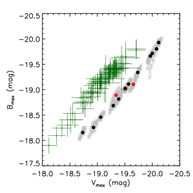
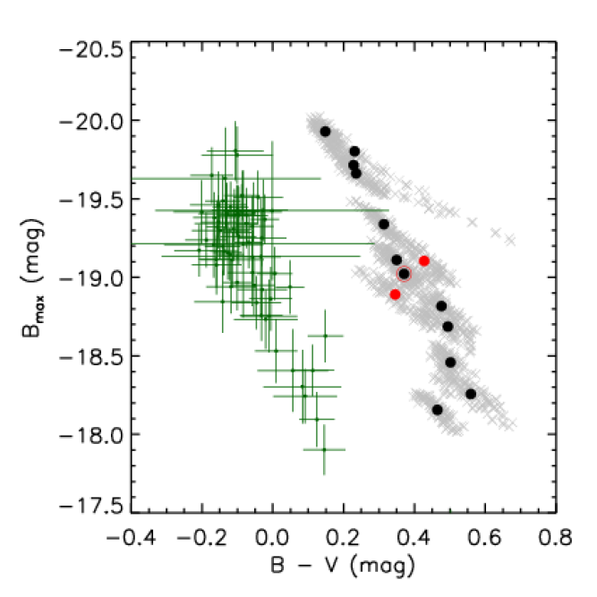
Figure 4: Comparison of synthetic light curve properties between our models and a sample of SNe Ia drawn from Hicken et al. (2009, excluding events with a distance modulus $\mu<33$ mag.). Left: Peak $B$-band versus peak $V$-band magnitude. Right: $B$-band magnitude versus $B-V$ colour at $t_{\rm max}^{B}$. Observations are shown as green crosses while measurements from our angle-averaged model light curves are shown as filled circles [black for our twelve models that differ only in the number and distribution of ignition sparks; red for our two models that adopt different central densities; model N100 is shown as a black circle with a red ring, for comparison to both sequences]. The light grey crosses indicated results from the full orientation dependent synthetic light curves (100 points for each model).

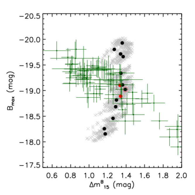
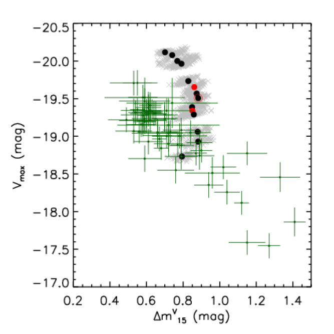
Figure 5: As Figure 4 but showing $B$- (left) and $V$-band (right) width-luminosity relations.

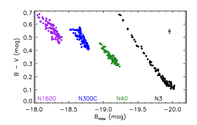
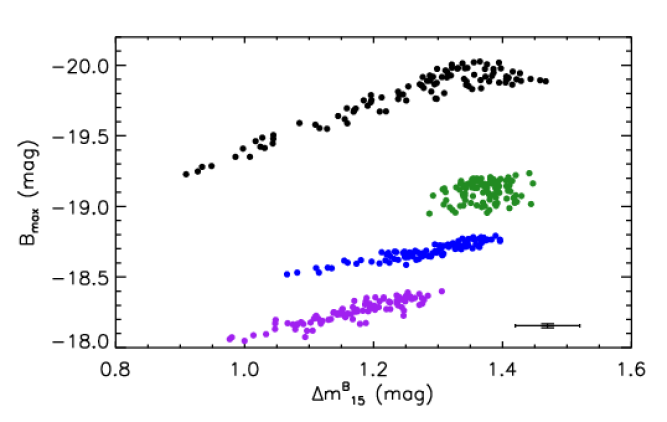
Figure 6: Correlations between light curve properties for different observer orientations: $B-V$ colour at peak versus $B_{\rm max}$ (left panel), $\Delta m_{15}^{B}$ versus $B_{\rm max}$ (right panel). In each case we show results for four of our models (N3, N40, N300C and N1600; see left panel for colour coding). The error bars shown in black indicate the uncertainties in our calculations owing to a combination of Monte Carlo noise and the length of our simulation timesteps.

3.2 Spectra

We now turn our attention to comparing spectral features in our models to observations. In this section, we will carry out comparisons without reference to absolute brightness or broad-band colours – comparisons of spectral features and light curve properties will be drawn together in Section 4.

3.2.1 Angle-averaged spectra

In Figure 7 we show angle-averaged synthetic spectra for four of our explosion models at four epochs (7, 17, 23 and 33 days after explosion). In all our models, both the early (e.g. 7 days post explosion) and maximum light (roughly $17$ days post explosion) spectra show clear spectral features associated with intermediate mass elements (e.g. Si and S), as are characteristic of SNe Ia.

The strong Si ii 6355-Å line and the weaker Si ii 5972-Å line both show clear systematic variation along our model sequence. In the 7 and 17 day spectra, both lines are stronger in the fainter models. The variation in the Si ii 5972-Å line is greater, meaning that the ratio of the equivalent widths (EWs) of the two Si lines [EW(5972-Å)/EW(6355-Å)] clearly varies with luminosity, as is observed (Nugent et al., 1995; Hachinger et al., 2008). As time passes, the Si velocities decrease and the lines become weaker. In our 33 day spectra, the Si and S lines have largely disappeared – the spectral formation is dominated by fluorescence in iron-group material, although there are still clear Ca features (including the H and K resonance features and the IR triplet).

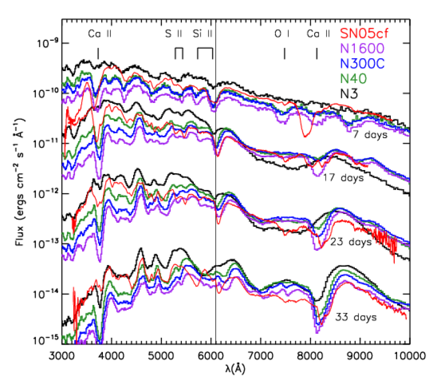
Figure 7: Synthetic spectra for models N3, N40, N300C and N1600 for 7, 17, 23 and 33 days after explosion (distance of 1 Mpc). For clarity, the spectra have been shifted via multiplicative factors of [20 (for 7 days), 1 (for 17 days), 1/20 (for 23 days) and 1/400 (for 33 days)]. Positions of characteristic features due to intermediate mass elements in the synthetic spectra are marked. A vertical line is drawn as a reference point for comparing velocities of the Si ii 6355Å line. For comparison, we also show spectra of the spectroscopically normal SNe Ia 2005cf (Garavini et al. 2007; red lines) for epochs of -10, +0, +6.5 and +16.5 days relative to $B$-band maximum, roughly comparable with the epochs of the synthetic spectra shown. The observed spectra have been corrected for redshift and reddening (using values from Pastorello et al. 2007) and scaled to account for the distance modulus and multiplicative factors applied to the model spectra.

Table 2: Parameters from measurements and fits to our synthetic spectra. MC noise and identification of continuum limit the accuracy of measuring $v_{\rm Si}(t_{\rm max}^{B})$ and $\dot{v}_{\rm Si}$ to around $\sim 300$ km s^-1 and 50 km s^-1 day^-1, respectively. For the snid matches we quote the SN name followed by the epoch of the observed spectrum (in days, relative to maximum light). In every case we give only the best matching (highest $r$lap) example. With the exception of the latest epoch considered for N1600C, all the best snid matches are to spectroscopically normal SNe Ia (as classified in the snid database).

			$t=t_{\rm max}^{B}-7$ days			$t=t_{\rm max}^{B}$			$t=t_{\rm max}^{B}+7$ days
Model	$v_{\rm Si}(t_{\rm max}^{B})$	$\dot{v}_{\rm Si}$a	$r{\rm lap}$	snid	$z$	$r{\rm lap}$	snid	$z$	$r{\rm lap}$	snid	$z$
	($10^{3}$ km s-1)	(km s-1 day-1)		match			match			match
N1	15.9	$70$	11.7	94D($-9.2$)	$-0.009$	7.8	06X($+2.3$)	$-0.003$	5.6	96bo($+9.2$)	$-0.008$
N3	14.7	$110$	12.1	96bl($-4.0$)	$-0.008$	8.5	02hd($+1.4$)	$-0.009$	6.4	07bm($+9.6$)	$-0.009$
N5	14.1	$70$	12.7	96bl($-4.0$)	$-0.005$	9.5	94T($+0.8$)	$-0.005$	6.9	04eo($+7.8$)	$-0.008$
N10	14.0	$80$	14.1	96bl($-4.0$)	$-0.005$	8.9	94T($+0.8$)	$-0.005$	7.7	04eo($+7.8$)	$-0.007$
N20	12.9	$120$	15.4	07au($-4.7$)	$-0.006$	9.2	02hd($+1.4$)	$-0.004$	8.2	04eo($+7.8$)	$-0.005$
N100H	13.3	$190$	17.2	02bo($-4.8$)	$-0.002$	7.6	04eo($+2.9$)	$-0.008$	9.1	07hj($+8.2$)	$-0.005$
N40	12.9	$190$	22.6	02bo($-4.8$)	$-0.002$	9.7	04eo($+2.9$)	$-0.007$	9.4	07hj($+8.2$)	$-0.003$
N100	12.9	$220$	21.8	02bo($-4.8$)	$-0.002$	9.8	04eo($+2.9$)	$-0.007$	9.5	07hj($+8.2$)	$-0.003$
N150	12.5	$190$	21.4	07au($-4.7$)	$-0.007$	7.8	04eo($+2.9$)	$-0.006$	8.9	07hj($+8.2$)	$-0.002$
N100L	12.4	$200$	18.8	02er($-7.0$)	$-0.002$	10.5	04eo($+2.9$)	$-0.006$	9.1	07hj($+8.2$)	$-0.002$
N300C	12.6	$200$	21.7	07au($-5.6$)	$-0.006$	9.6	04eo($+2.9$)	$-0.006$	9.2	07hj($+8.2$)	$-0.002$
N200	12.2	$260$	19.4	02bo($-4.8$)	$-0.001$	11.6	04eo($+2.9$)	$-0.005$	8.6	07hj($+8.2$)	$-0.000$
N1600	11.9	$260$	15.5	02er($-5.0$)	$-0.004$	9.4	04eo($+2.9$)	$-0.005$	8.7	07hj($+8.2$)	$0.000$
N1600C	11.4	$300$	14.5	08ar($-6.6$)	$0.000$	9.1	04eo($+2.9$)	$-0.003$	10.5	02es($+9.0$)b	$-0.009$

^a $\dot{v}_{\rm Si}$ parametrizes the rate of evolution of the Si ii 6355Å line at epochs around $t_{\rm max}^{B}$ (see Equation 1).
^b 91bg-like

We have measured the blue-shift velocity ($v_{\rm Si}$) of the Si ii 6355-Å line at $t_{\rm max}^{B}$ for each model (given in Table 2). In addition, we have also measured the line velocity for times between seven days before and six days after $t_{\rm max}^{B}$ (as noted above, the line generally fades from the spectrum soon thereafter). These measurements are shown for a sub-set of models in Figure 8. Since the evolution is fairly simple, we have also fit a linear function to each model:

$${v}_{\rm Si}(t)=v_{\rm Si}(t_{\rm max}^{B})-\dot{v}_{\rm Si}\times(t-t_{\rm max}^{B})\;\;.$$ (1)

Although simple, such fits provide a convenient rate-of-decrease parameter ($\dot{v}_{\rm Si}$) that can be compared between all the models. The derived values of $\dot{v}_{\rm Si}$, which have a MC uncertainty of ${\sim}50$ km s^-1 day^-1, are given in Table 2 and sample fits are shown in Figure 8.

The range of blueshift $v_{\rm Si}(t_{\rm max}^{B})$ covered by our models ($11,400$ to $15,900$ km s^-1) is roughly compatible with the maximum light velocities observed for normal SNe Ia [${\sim}10,000$ to $14,000$ km s^-1; see, e.g., figure 1 of Benetti et al. (2005); further discussion below]. As might be expected based on the correlation between kinetic energy and ⁵⁶Ni mass (see Table 1), the brighter models have higher $v_{\rm Si}(t_{\rm max}^{B})$. The mean rate of line-velocity evolution ($\dot{v}_{\rm Si}$) also varies systematically along the model sequence – the velocity decreases most rapidly in the faintest models. Quantitative comparison between our $\dot{v}_{\rm Si}$-values and the velocity evolution parameters in Benetti et al. (2005) is not easy because their measurements do not correspond to a fixed range of epochs. However, qualitative comparison consistently suggest that our synthetic spectra evolve too quickly: in our spectra, the Si line is typically weak or absent within a week of maximum light while Benetti et al. (2005) report many detections up to three or four weeks after $B$-band maximum (but see also van Rossum 2012).

Figure 7 clearly illustrates verisimilitude between our synthetic spectra and observations of normal SNe Ia (exemplified by SN2005cf). However, there are also clear discrepancies in the spectral features (e.g. around the Ca ii IR triplet). Consequently, it is interesting to consider whether our model spectra would lead to classification as normal SNe Ia or whether they provide a better match to one or other spectroscopically peculiar sub-class of SNe Ia. To investigate this, we provide a rough classification of our synthetic spectra by using snid (Blondin & Tonry, 2007).

snid is widely used in the classification of newly discovered SNe. It operates by first fitting and removing a pseudo-continuum from the spectra and then comparing the features in the flattened spectra to template SNe Ia. This approach removes the sensitivity to absolute brightness and (largely) to colour, focussing instead on the spectral features. Consequently, some caution must be applied when interpreting the results (a good match in spectral features must be accompanied by agreement in light curve properties to constitute a good model). snid comparisons nevertheless provide an excellent means to compare spectral features, the procedure by which observational classification is made. snid returns both a list of SN templates that are well-matched to the input spectrum along with a goodness-of-fit statistic ($r{\rm lap}$-value), which is based on the correlation between the input spectrum and the template (larger $r{\rm lap}$ values correspond to better matches; $r{\rm lap}>5$ is considered a “good” match; Blondin & Tonry 2007). . The code also fits for a redshift parameter ($z$), based on comparison to the templates. When analysing models, this parameter can be viewed as a means to quantify any systematic velocity offset between features in the model and observations (see below). We made our comparisons to a database of 3754 spectra of 349 template SNe Ia (version 2.0 of the snid template database, which includes data from Blondin et al. 2012).

Following an approach similar to Blondin et al. (2011), we ran snid on angle-averaged synthetic spectra for three epochs for each of our models: at $t_{\rm max}^{B}$ and at both one week before and one week after $t_{\rm max}^{B}$. In all cases, we restricted the wavelength range of comparison to $3500<\lambda($Å$)<8500$, forced the redshift associated with our synthetic spectra to be small and allowed comparison to template spectra for which the epoch (relative to maximum light) was within $\pm 3$ days of the synthetic spectrum. Sample results from our snid fits are presented in Table 2 and Figure 9. In all cases, our spectra yielded acceptable ($r{\rm lap}>5$) matches to multiple SNe. For brevity, we tabulate only the best match SN in each case (see Table 1, which gives the SN name, epoch of the matched template, $r{\rm lap}$-value and redshift parameter for the best match to each synthetic spectrum). Note that since each of our snid runs was carried out independently without restriction to any particular sub-set of the database, the best matching SN identified for a given model is not the same at all epochs considered. This is not particularly surprising – from Section 3.1, it is clear that the time evolution of the models is imperfect. Moreover, it does not imply that insisting on comparison to one particular object leads to poor $r{\rm lap}$-values. This is illustrated for one of our models in Figure 9, which shows snid comparisons between N40 and SN2004eo at all three epochs analysed (we chose this comparison object since it is the best match at $t_{\rm max}^{B}$).

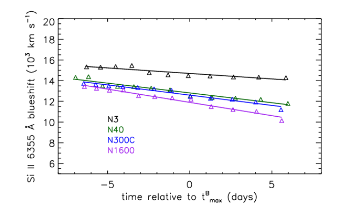
Figure 8: Evolution of the blueshift of the Si ii 6355Å line for models N3, N40, N300C and N1600. Symbols show measurements from our synthetic spectra, which typically have an uncertainty of $\sim 300$ km s^-1 due to MC noise and choice of continuum level. The solid lines show the simple linear fits used to characterise the rate of evolution at these epochs.

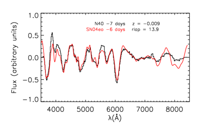
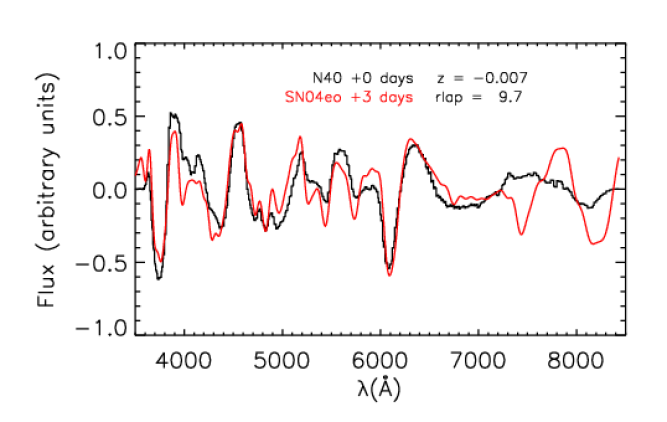
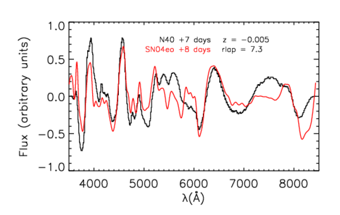
Figure 9: snid comparison of spectral features in our N40 model to SN2004eo (the best match supernova identified for our N40 maximum light spectrum). We show results for three epochs, $-7$, $0$ and $+7$ days relative to maximum light in $B$ band. The epoch of the relevant observation, the $r{\rm lap}$-value of the match and the redshift parameter ($z$), is indicated in each panel. The spectra are shown flattened, as they are compared by snid (i.e. after a pseudo continuum has been fit and subtracted). Small red-shifts are allowed in identifying the best correlation. These are included here and can be used to quantify the typical mismatch in velocities between the models and observations (see text and Table 2).

In all cases, at $t_{\rm max}^{B}$ and one week before $t_{\rm max}^{B}$, the best snid match is with a template for a normal SNe Ia (according to the classifications in the snid database). Moreover, the quality of the fit is generally good ($r{\rm lap}>7$ in all cases) and it is best for the models with moderate numbers of ignition sparks (N40, N100, N100L, N100H – i.e. the same models which were most promising based on their light curve characteristics, see Section 3.1). We do note, however, that the models often fail to match well in the redder parts of the spectrum (around O i 7774 Å and the Ca ii IR triplet, particularly at the later epochs). Both for models with many fewer or many more ignition sparks, the best $r{\rm lap}$ value is generally poorer but still sufficiently high that, if realised in nature, such models would be spectroscopically classified as SNe Ia.

At the later epoch (one week after $t_{\rm max}^{B}$), the best match is still with a normal SN Ia for most models. At this epoch, the $r{\rm lap}$ value is typically slightly poorer although still good for our models with intermediate deflagration strengths (N40 – N100). For our very faintest model, the best post-maximum match is to a 91bg-like SN Ia. This match with a peculiar SNe Ia at the extreme of our model sequence is not particularly informative, however – based on the light curves (i.e. absolute brightnesses), we can easily exclude our models with the largest numbers of ignition sparks from being appropriate for the bulk of normal SNe Ia. Physical correspondence with 91bg-like SNe at the extreme of our model sequence is also unlikely based on light curves: our N1600 and N1600C models show slow post-maximum decline rates (the smallest $\Delta m_{15}^{B}$-values amongst our models), while observed 91bg-like SNe Ia are noted for their rapid decline after maximum light.

We note that for none of our comparisons was the best snid match with a 1991T-like SN Ia. Considering our five models with high ⁵⁶Ni mass (N1, N3, N5, N10 and N20), the best $r{\rm lap}$-values in comparisons to 1991T-like events were only 7.4, 5.3 and 5.4 respectively for the $-7$, $0$ and $+7$ day epochs considered. These are substantially poorer than the matches found for spectroscopically normal SNe Ia (see Table 2), suggesting that our models are not particularly promising candidates to explain 1991T-like events.

Our snid fits also allow us to more accurately assess the extent to which the line velocities that manifest in our spectra agree with observations. The best correlation is generally obtained when a small blueshift is applied to the template spectra, meaning that the velocities in the simulations are slightly too high (typically by around 1500 km s^-1 for maximum light spectra). This systematic effect suggests that slightly too much kinetic energy is typically released. This might be a consequence of the assumed initial WD composition in our models. In particular, a smaller C/O ratio could lead to less energy generation and more slowly expanding ejecta – this will be considered further in a forthcoming study.

3.2.2 Orientation dependence of spectra

Figure 10 shows synthetic spectra for models N40 and N3 at four epochs for three example observer orientations, which correspond to the directions in which the peak bolometric magnitude was largest, smallest and close to the median value.

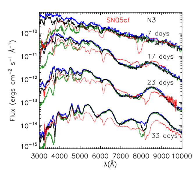
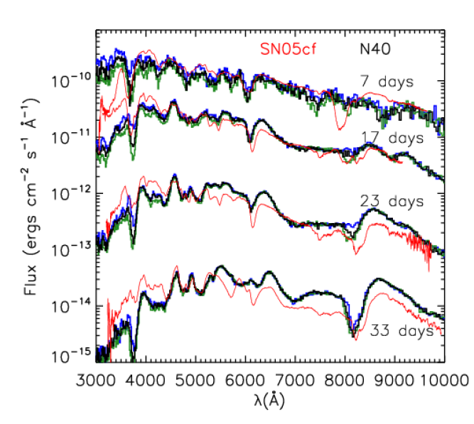
Figure 10: Orientation-dependent spectra for models N3 and N40 for 7, 17, 23 and 33 days after explosion (distance of 1 Mpc). In black (blue/green) we show spectra representative of orientations with median (maximum/minimum) brightness. As in Figure 7, the spectra have been shifted via multiplicative factors for clarity and observations of SN 2005cf are shown in red.

As expected based on the discussion of light curves in Section 3.1.2, our synthetic spectra for model N40 are not very sensitive to the observer orientation (only the region around the Ca ii infrared triplet and the blue/ultraviolet region of the spectrum are noticeably affected). In particular, neither the strength nor blueshift of the Si ii $6355$-Å feature is significantly direction dependent. This degree of orientation dependence is characteristic of our models with moderate to large numbers of ignition sparks.

In contrast, the N3 spectral features do vary noticeably with orientation. At maximum light, the Si ii $6355$-Å  feature is less blueshifted (down to $v_{\rm Si}\sim 13,500$ km s^-1) and weaker for orientations in which the total flux is higher. For the median brightness and brightest example spectra of model N3 around $t_{\rm max}^{B}$, the best snid matches are still to normal SNe Ia, as for the angle-averaged spectrum of this model. In contrast, the faint spectrum shows a strongest correlation with a SN Ic (SN 04aw), having $r$lap = 7.5 (the best match with a SN Ia has $r$lap = 5.7). However, we stress that the absolute brightness of model N3 (see Section 3.1) is too large for this to be a good model for a normal SN Ia or SN Ic. Therefore, accounting for orientation dependence does not alter our conclusion that the brightest models do not appear well-matched to any observed class of SN (see below).

4 Discussion

In the previous sections we have presented our synthetic light curves and spectra and compared them to the observed properties of normal SNe Ia. Here, we draw together the results of these comparisons and discuss their implications for the model parameters explored in our study. We also compare some key results to those obtained in previous studies of DDT models.

4.1 Role of the strength of the deflagration phase

Twelve of our fourteen models differ from each other only in the geometry with which the initial deflagration was ignited. These produce a sequence of models with differing deflagration strengths and final ⁵⁶Ni masses ranging from 0.32 – 1.1 M_⊙. Based on comparison of spectral features alone, almost all models in this sample invite comparison with normal SNe Ia: apart from exceptions at the extremes of our model sequence, all our snid analyses yielded best matches to normal SNe Ia, with respectable $r$lap-values (particularly at early epochs).

When we also consider light curve information, however, a clearer discrimination between our models emerges and our analyses consistently point to the best agreement with observations for the models with intermediate strengths of the deflagration phase (e.g. N40, N100). These models have roughly the right rise time ($t^{B}_{\rm max}$), light curve decline parameter ($\Delta m_{15}^{B}$), peak luminosity and peak $V-R$ colour to match normal SNe Ia. The correspondence with observations is nevertheless imperfect – for these models, important difficulties include matching the $I$ band light curve and the peak $B-V$ colours, which are systematically too red (see Section 4.5). In addition, we consistently find that the models evolve too quickly post-maximum (e.g., although close, both the light curve decline parameters $\Delta m_{15}^{B}$ and $\Delta m_{15}^{V}$ are a little larger than in the bulk of normal SNe Ia; see Figure 5).

Although our models with weak deflagrations (i.e. those with very small numbers of ignition sparks: N1, N3, N5) do have bluer $B-V$ colour at peak than our models with stronger deflagrations, they are still too red compared to the bulk of normal SNe Ia (see Figure 4). Especially in $V$-band, the N1, N3 and N5 light curves are somewhat too bright for most normal SNe Ia and of particular note is the failure of these models to yield slower post-maximum evolution compared to their fainter counterparts (recall that normal SNe Ia, and also 1991T-like SNe Ia, are observed to obey a clear correlation between peak luminosity and light curve width); this suggests that our model sequence does not correctly capture the processes that drive systematically slower evolution in brighter objects (see Section 4.4 below). In addition, our models with few ignition sparks can be subject to very significant asymmetries that lead to orientation effects that are inconsistent with observations (see Section 4.3 below). Taken together, these shortcomings lead us to disfavour our models with weak deflagration phases as promising matches to normal SNe Ia. Furthermore, at present, we are not aware of any proposed sub-class of SNe Ia that displays photometric properties similar to these models.

In comparison to normal SNe Ia, our models with very strong deflagration phases fare somewhat better than those with weak deflagrations but are still inferior to the models around the middle of our sequence. In particular, N1600 and N1600C have $B_{\rm max}$-values that are clearly sub-luminous despite having $V_{\rm max}$ and $R_{\rm max}$ that are close to those of spectroscopically normal SNe Ia. Despite being relatively faint, these models actually show the slowest post-maximum decline (smallest $\Delta m_{15}^{B}$) in our sequence. This is in sharp contrast to the sub-luminous 1991bg-like SNe, which typically display rapid post-maximum decline (see e.g.  Taubenberger et al., 2008) in addition to spectroscopic peculiarities. Relatively gradual fading is observed in 2002cx-like SNe (sub-luminous SNe Ia characterised by low expansion velocities; see e.g. Branch et al. 2004; Jha et al. 2006). However, as mentioned in Section 1, the best models for 2002cx-like SNe appear to be pure deflagration events (Branch et al., 2004; Jha et al., 2006; Phillips et al., 2007; Jordan et al., 2012; Kromer et al., 2013). We note that it was to be expected that our simulations with large numbers of ignition sparks bear some resemblance to pure deflagration models (e.g. very red colours and relatively slow post-maximum decline): as the number of ignition sparks is increased in our DDT models, the deflagration phase becomes increasingly dominant in the explosion.

4.2 Role of central density

Three of our models (N100, N100H and N100L) differ from each other only in the choice of the central density of the WD. As would be expected from the differences in ⁵⁶Ni mass, the peak brightnesses of these models are only moderately different from each other (spanning a range of only ${\sim}0.3$ mag in $V$ band). Therefore, for our model sequence, we conclude that the influence of the central density on the observables is of secondary importance to deflagration strength. Nevertheless, the effect of central density is potentially observable and it could act as a secondary parameter (e.g.  Höflich et al., 2010; Krueger et al., 2010; Seitenzahl et al., 2011; Krueger et al., 2012; Calder et al., 2013). We do note that, in our simulations, there is a weak but systematic trend for redder $B-V$ colour with increasing central density, a consequence of the larger mass of iron-group elements produced. Thus, variations in central density could drive dispersion in e.g. the colours of SNe Ia produced via DDT events.

4.3 Orientation effects

The light curves for all our models show some sensitivity to the observer inclination angle: in particular, we obtain more rapid post-maximum decline for orientations in which the explosion is seen to be brighter. This leads to a predicted anti-correlation between $\Delta m_{15}^{B}$ and $B_{\rm max}$ for the same explosion viewed from different directions. Such a correlation is opposite to the sense of the observed WLR for normal SNe Ia (but characteristically similar to that due to orientation effects in other asymmetric models; see e.g. Sim et al. 2007). Consequently, orientation effects in these models cannot play a role in explaining the primary trend of the SN Ia WLR.

In our most asymmetric model (N3), the scale of the orientation effect is so large that it can be used to effectively exclude the model as being viable for normal SNe Ia. However, in the other models (particularly those with modest to large numbers of ignition sparks), the effects of orientation are comparable to the scatter about the observed WLR and may therefore provide a satisfactory explanation for the observed spread around the mean WLR.

4.4 The light curve width luminosity relation in our models

Viewed as a sequence, our DDT simulations do not show a clear WLR, in contrast to observations of normal SNe Ia (see Figure 5). In particular, although they span a range of $B_{\rm max}$ and $V_{\rm max}$ that is wide enough to cover the whole range of observed luminosities for normal SNe Ia, all our models have very similar post-maximum decline rate parameters $\Delta m_{15}^{B}\sim 1.3$ mag. The implication of this is that varying the strength of the deflagration alone (as parametrized by the ignition configuration) does not necessarily lead to a sequence of models that populate the light curve parameter space occupied by normal SNe Ia.

Previous theoretical studies of sets of one- and two-dimensional DDT models and associated synthetic observables have produced WLRs that are roughly consistent with observations. For example, Höflich & Khokhlov (1996) show that their 1D delayed detonation models follow a width luminosity relation. However, along their sequence of models the variation is not in the ignition conditions but in their choice for when the transition to detonation occurs (parametrized in terms of a transition density). This is also true for the 1D models recently analysed by Blondin et al. (2013) but is quite different from our sequence of 3D models in which the DDT criterion is not tuned (i.e the parameters that enter our model for the DDT mechanism are held fixed), but rather the parametrized ignition configuration is used to control the deflagration strength.

In their set of 2D models, Kasen et al. (2009) varied parameters for both the ignition configuration and the DDT criterion. Careful analysis by Blondin et al. (2011) showed that many of the Kasen et al. (2009) models (excluding very asymmetric setups) provide good matches to SNe Ia and that the set of models populates the space of the observed SN Ia WLR reasonably well (e.g. figure 7 of Blondin et al. 2011). However, we note that their models do show a correlation between the DDT parameter used and the light curve width parameter $\Delta m_{15}^{B}$. In particular, while their models with their fourth and fifth DDT criteria (dc4 and dc5 sequences; Kasen et al. 2009; Blondin et al. 2011) have, on average, $\Delta m_{15}^{B}\sim 1.3$ (i.e. similar to our models), only their models in the dc1 and dc2 sequences typically yield $\Delta m_{15}^{B}\,\hbox{\lower 2.58334pt\hbox{$\sim$}\hbox to0.0pt{\hss\raise 2.58334pt\hbox{$<$}}}\,1$, which is characteristic of the observed SNe Ia that are missed by our calculations.

We therefore conclude that although varying the rate with which material is consumed during the deflagration phase has a large effect in DDT models, changing this alone does not produce a sequence of simulations that accounts for the observed variation amongst SNe Ia. Our results suggest that either (i) the deflagration strength is similar in most cases (being well-represented by our models with moderate numbers of ignition sparks) and the variations from object to object are controlled by an unrelated effect (e.g. stochasticity in the DDT process) (ii) some additional explosion property (e.g. progenitor metallicity or properties of the DDT mechanism) varies in a way that is strongly correlated with the strength of the deflagration (note that all parameters of our models were held fixed in this study except the deflagration ignition configuration and the WD central density); or (iii) Chandrasekhar-mass DDT models are not responsible for the bulk of normal SNe Ia.

4.5 Peak colours in our models

As noted in Section 3.1 and illustrated in Figure 4, our 3D DDT models are systematically too red compared to observations of normal SNe Ia (by around ${\sim}0.4$ mag in $B-V$ at $t_{\rm max}^{B}$). We attribute this to the location of iron-group elements (particularly the deflagration ash) in intermediate layers of the ejecta and we note that this occurs even for our models with central and near-symmetric ignition (such as N300C) – in none of the models was the deflagration ash prevented from floating towards the surface (Seitenzahl et al., 2013).

The Kasen et al. (2009) 2D models were also noted to be systematically too red, in that case by ${\sim}0.2$ mag in $B-V$ (Blondin et al., 2011). The problem of red colours is less significant in studies of 1D models. For example, Höflich et al. (1996) argue that, although slightly too red, their 1D DDT models yield $B-V$ colours that are consistent with observations, given uncertainties in the modelling. Similarly, the recent study of Blondin et al. (2013) also gives peak colours (they focus on $B-R$) that are within the range observed for normal SNe Ia (in contrast, as for $B-V$, our 3D models with moderate numbers of ignition sparks give $B-R$ at peak that is too red by ${\sim}0.3-0.5$ mag). As noted by Blondin et al. (2013), direct comparison is complicated here since the 1D simulations can include more sophisticated radiative transfer and ionization calculations than do our multi-dimensional models: non-LTE effects can influence the colours by a few tenths of a magnitude (Höflich et al., 1996; Kasen et al., 2009). Nevertheless, we do note that, even with our radiative transfer methods, we have obtained bluer colours for models that do not involve a deflagration phase [see e.g. Sim et al. (2010), Pakmor et al. (2012) and Röpke et al. (2012): in all those cases, models with peak $B-V\sim 0.2$ mag were found for luminosities corresponding to normal SNe Ia] and for the 1D Chandrasekhar mass W7 model, in which the stable iron-group elements are present but artificially restricted to low velocities (Kromer & Sim, 2009). Thus our modelling methods certainly predict that the differential effect of deflagration ash in 3D models is to induce redder colours, which may be a major challenge. Nevertheless, we acknowledge that the scale of this effect may be comparable to uncertainties introduced by assumptions in the modelling and further investigation is warranted.

5 Summary, implications and future work

We have presented synthetic light curves and spectra for a sequence of 3D DDT models for SNe Ia. Study of 3D effects is particularly important for DDT models owing to the complexity of modelling the buoyancy-unstable deflagration phase. Our models differ from each other in two important respects, both of which are therefore probed by our study: the strength of the deflagration phase (as parametrized by the number and location of the ignition sparks) and the central density of the WD star.

As described by Seitenzahl et al. (2013), the model sequence gives rise to explosions with a sufficiently wide range of ⁵⁶Ni masses to encompass the range covered by normal SNe Ia. This is confirmed by the range of brightnesses of our synthetic light curves, which also have rise times compatible with observations. Moreover, inspection of our synthetic spectra around maximum light shows a fairly good match to the observed spectral features of normal SNe Ia. Comparing our models clearly shows that variation in the strength of the deflagration flame can have a greater influence on the explosion and its synthetic observables than does the WD central density (which is varied by a factor of ${\sim}5$ in our study).

To interpret the results obtained from comparison of our models to observations, we return to the two purposes of our set of models (see Section 2.1): (i) to investigate whether good agreement with properties of a normal SNe Ia can be obtained for some choice of the parametrized ignition in our simulations and (ii) to explore whether variations in the deflagration strength can account for (a part of) the observed diversity of SNe Ia. With regard to (i), it is clear that the best match between any of our models and observations consistently occurs around the mid point of our sample (models N40, N100) and that, in many respect, such models fare rather well. In particular, these models show the best spectral match to normal SNe Ia (as parametrized by the snid $r$lap values) and have light curve rise times, peak brightnesses and decline timescales comparable to the bulk of normal SNe Ia. In addition, these models are sufficiently close to spherical symmetry that line-of-sight effects are modest – orientation effects in these models could explain the scatter across the observed WLR but do not lead us to reject the models. However, on detailed inspection, several shortcomings remain. In particular, our models predict line velocities that are systematically too high (by ${\sim}1500$ km s^-1 for Si ii at maximum light) and colours that are too red (by around 0.4 mag in $B-V$ at maximum light). While exploring initial WD models of differing composition may provide a solution to the velocity mismatch, we suggest that the red colours are a consequence of the distribution of iron-group elements in the models (in particular, the deflagration ash), which may be a significant concern. Further modelling of this is certainly warranted, including studies that fully explore the possible geometry and location of the deflagration ash in 3D simulations and that properly consider the sensitivity of conclusions to approximations made in the radiative transfer (including a more sophisticated treatment of non-LTE effects).

The implication of our models for point (ii) are clearer. The level of agreement between our synthetic observables and normal SNe Ia becomes poorer at both ends of our model sequence. Moreover, our models show little systematic variation in light curve decline rates along the model sequence (Figure 5). Thus, viewed as a complete set, our models do not reproduce the observed SN Ia WLR. While uncertainties in the modelling may account for systematic shortcomings in the models (e.g. absolute mismatches in colours or velocities as mentioned above), it is to be expected that predictions for differential effects along the model sequence are more robust. Consequently, we suggest that the failure of our models to predict any strong WLR indicates that either the rate of fuel consumption during the deflagration phase is not the primary parameter driving the variation between explosions in a population of SNe Ia produced via the DDT Chandrasekhar-mass scenario, or that the observed population of SNe Ia is not dominated by events from this explosion channel. Further investigation of the sensitivity of 3D simulations to other aspects of the modelling, e.g. the choice of DDT criterion (as has been done in 1D and 2D), are needed to explore this further.

It is noteworthy that our models with few ignition sparks (N1, N3) fare most poorly in comparison with observations of SNe Ia (they are typically too bright and can show strong orientation effects that are inconsistent with the observed tightness of the WLR). As noted in Section 2.1, our calculations are not based on any particular ignition simulations for SNe Ia. However, among our models, N1 and N3 are likely the best representations of explosions with single-spot off-centre ignition (in contrast, our models with larger numbers of sparks are more likely appropriate for centrally ignited explosions; see Seitenzahl et al. 2013). In light of recent studies that favour ignition of the deflagration at an off-centre point (Zingale et al., 2009; Nonaka et al., 2012), the shortcomings of our models with few sparks therefore pose a particular challenge to the Chandrasekhar-mass DDT scenario for normal SNe Ia. This lends credence to the alternative scenario in which off-centre ignition of a Chandrasekhar mass WD leads to explosion via pure deflagration (i.e. no DDT occurs), giving rise to faint spectroscopically-peculiar transients rather than normal SNe Ia (Kromer et al., 2013).

Even if Chandrasekhar-mass DDT models are not appropriate for the bulk of normal SNe Ia, such explosions might still be present in the population, and our models can therefore be used to guide their identification. For example, Foley et al. (2012) provided evidence that SNe Ia with circumstellar material (detected via blue-shifted Na i absorption) have preferentially higher Si ii velocities and redder colours than the average SN Ia. Here, a tantalising correspondence arises since, as noted above, our models do manifest both high line velocities and red colours. Also, our models are appropriate for the Chandrasekhar-mass single-degenerate scenario, the channel for which it has been claimed that blue-shifted Na i absorption can be most readily explained (see e.g. Patat et al. 2007; Sternberg et al. 2011, but see also Shen et al. 2013; Soker et al. 2013). However, further study is needed and we caution that both the line velocities and colours may be subject to significant systematic uncertainties due to assumptions of the modelling.

Finally, we reiterate the continuing need for improving the accuracy of modelling. As noted by e.g. Blondin et al. (2013), currently a trade off is often made between 1D studies (in which spherical symmetry is imposed as an ad hoc assumption; e.g. Höflich et al. 1996; Blondin et al. 2013) and multi-D studies (in which cruder approximations in the radiative transfer are made necessary by considerations of computational expediency: e.g. Kasen et al. 2006, Kromer & Sim 2009, Kasen et al. 2009, this study). It is clear, however, that the agreement between several explosion models (including Chandrasekhar-mass DDT models) and observations of SNe Ia is sufficiently close that detailed evaluation can be limited by the accuracy of modelling assumptions (see e.g.  Röpke et al., 2012). For example, realistic modelling of departures from LTE is important in SNe Ia, particularly during the post-maximum decline phase (e.g., compared to the typical error associated with measurements of $\Delta m_{15}^{B}$, the $B$-band light curve evolution is quite sensitive to the non-LTE treatment of ionization; see e. g. Kromer & Sim 2009). Such modelling sensitivity must be borne in mind when comparing calculations to data. At the same time, multi-D studies show that asymmetries in realistic explosion models affect synthetic light curves and spectra by observable amounts, particularly (but not exclusively) in the blue and ultraviolet regions (e.g. the $\Delta m_{15}^{B}$-spread due to orientation effects in our models is comparable to the observed dispersion about the SNe Ia WLR). Consequently, if theoretical predictions are to match the quality of data provided by current SN Ia observational programs, there remains a clear need for ongoing development of modelling tools that should ultimately include both the best possible micro-physics and handle the most realistic, multi-dimensional explosion models.

References

- Benetti et al. (2005) Benetti S. et al., 2005, ApJ, 623, 1011
- Blondin et al. (2013) Blondin S., Dessart L., Hillier D. J., Khokhlov A. M., 2013, MNRAS, 429, 2127
- Blondin et al. (2011) Blondin S., Kasen D., Röpke F. K., Kirshner R. P., Mandel K. S., 2011, MNRAS, 417, 1280
- Blondin et al. (2012) Blondin S. et al., 2012, AJ, 143, 126
- Blondin & Tonry (2007) Blondin S., Tonry J. L., 2007, ApJ, 666, 1024
- Branch et al. (2004) Branch D., Baron E., Thomas R. C., Kasen D., Li W., Filippenko A. V., 2004, PASP, 116, 903
- Bravo & García-Senz (2008) Bravo E., García-Senz D., 2008, A&A, 478, 843
- Bravo & García-Senz (2009) Bravo E., García-Senz D., 2009, ApJ, 695, 1244
- Bravo et al. (2009) Bravo E., García-Senz D., Cabezón R. M., Domínguez I., 2009, ApJ, 695, 1257
- Calder et al. (2013) Calder A. C., Krueger B. K., Jackson A. P., Townsley D. M., 2013, Frontiers of Physics, 8, 168
- Ciaraldi-Schoolmann et al. (2013) Ciaraldi-Schoolmann F., Seitenzahl I. R., Roepke F. K., 2013, ArXiv e-prints
- Elias et al. (1985) Elias J. H., Matthews K., Neugebauer G., Persson S. E., 1985, ApJ, 296, 379
- Foley et al. (2012) Foley R. J. et al., 2012, ApJ, 752, 101
- Gamezo et al. (2003) Gamezo V. N., Khokhlov A. M., Oran E. S., Chtchelkanova A. Y., Rosenberg R. O., 2003, Science, 299, 77
- Ganeshalingam et al. (2011) Ganeshalingam M., Li W., Filippenko A. V., 2011, MNRAS, 416, 2607
- Garavini et al. (2007) Garavini G. et al., 2007, A&A, 471, 527
- Golombek & Niemeyer (2005) Golombek I., Niemeyer J. C., 2005, A&A, 438, 611
- Hachinger et al. (2008) Hachinger S., Mazzali P. A., Tanaka M., Hillebrandt W., Benetti S., 2008, MNRAS, 389, 1087
- Hayden et al. (2010) Hayden B. T. et al., 2010, ApJ, 712, 350
- Hicken et al. (2009) Hicken M. et al., 2009, ApJ, 700, 331
- Hillebrandt et al. (2013) Hillebrandt W., Kromer M., Röpke F. K., Ruiter A. J., 2013, Frontiers of Physics, 8, 116
- Hillebrandt & Niemeyer (2000) Hillebrandt W., Niemeyer J. C., 2000, Ann. Rev. Astron. Astrophys., 38, 191
- Höflich & Khokhlov (1996) Höflich P., Khokhlov A., 1996, ApJ, 457, 500
- Höflich et al. (1996) Höflich P., Khokhlov A., Wheeler J. C., Phillips M. M., Suntzeff N. B., Hamuy M., 1996, ApJL, 472, L81
- Höflich et al. (1995) Höflich P., Khokhlov A. M., Wheeler J. C., 1995, ApJ, 444, 831
- Höflich et al. (2010) Höflich P. et al., 2010, ApJ, 710, 444
- Jha et al. (2006) Jha S., Branch D., Chornock R., Foley R. J., Li W., Swift B. J., Casebeer D., Filippenko A. V., 2006, AJ, 132, 189
- Jordan et al. (2012) Jordan IV G. C. et al., 2012, ApJ, 759, 53
- Jordan et al. (2012) Jordan IV G. C., Perets H. B., Fisher R. T., van Rossum D. R., 2012, ApJL, 761, L23
- Kasen (2006) Kasen D., 2006, ApJ, 649, 939
- Kasen et al. (2009) Kasen D., Röpke F. K., Woosley S. E., 2009, Nature, 460, 869
- Kasen et al. (2006) Kasen D., Thomas R. C., Nugent P., 2006, ApJ, 651, 366
- Khokhlov et al. (1992) Khokhlov A., Mueller E., Hoeflich P., 1992, A&A, 253, L9
- Khokhlov (1991) Khokhlov A. M., 1991, A&A, 245, 114
- Kozma et al. (2005) Kozma C., Fransson C., Hillebrandt W., Travaglio C., Sollerman J., Reinecke M., Röpke F. K., Spyromilio J., 2005, A&A, 437, 983
- Krisciunas et al. (2004) Krisciunas K., Phillips M. M., Suntzeff N. B., 2004, ApJL, 602, L81
- Kromer et al. (2013) Kromer M. et al., 2013, MNRAS, 429, 2287
- Kromer & Sim (2009) Kromer M., Sim S. A., 2009, MNRAS, 398, 1809
- Kromer et al. (2010) Kromer M., Sim S. A., Fink M., Röpke F. K., Seitenzahl I. R., Hillebrandt W., 2010, ApJ, 719, 1067
- Krueger et al. (2012) Krueger B. K., Jackson A. P., Calder A. C., Townsley D. M., Brown E. F., Timmes F. X., 2012, ApJ, 757, 175
- Krueger et al. (2010) Krueger B. K., Jackson A. P., Townsley D. M., Calder A. C., Brown E. F., Timmes F. X., 2010, ApJL, 719, L5
- Kurucz & Bell (1995) Kurucz R. L., Bell B., 1995, Atomic line list
- Lucy (2002) Lucy L. B., 2002, A&A, 384, 725
- Lucy (2003) Lucy L. B., 2003, A&A, 403, 261
- Lucy (2005) Lucy L. B., 2005, A&A, 429, 19
- Ma et al. (2013) Ma H., Woosley S. E., Malone C. M., Almgren A., Bell J., 2013, ApJ, 771, 58
- Mazzali et al. (2007) Mazzali P. A., Röpke F. K., Benetti S., Hillebrandt W., 2007, Science, 315, 825
- Meikle (2000) Meikle W. P. S., 2000, MNRAS, 314, 782
- Nomoto et al. (1984) Nomoto K., Thielemann F.-K., Yokoi K., 1984, ApJ, 286, 644
- Nonaka et al. (2012) Nonaka A., Aspden A. J., Zingale M., Almgren A. S., Bell J. B., Woosley S. E., 2012, ApJ, 745, 73
- Nugent et al. (1995) Nugent P., Phillips M., Baron E., Branch D., Hauschildt P., 1995, APJL, 455, L147+
- Pakmor et al. (2012) Pakmor R., Kromer M., Taubenberger S., Sim S. A., Röpke F. K., Hillebrandt W., 2012, ApJL, 747, 10
- Pastorello et al. (2007) Pastorello A. et al., 2007, MNRAS, 376, 1301
- Patat et al. (2007) Patat F. et al., 2007, Science, 317, 924
- Phillips et al. (2007) Phillips M. M. et al., 2007, PASP, 119, 360
- Plewa et al. (2004) Plewa T., Calder A. C., Lamb D. Q., 2004, ApJ, 612, L37
- Reinecke et al. (2002) Reinecke M., Hillebrandt W., Niemeyer J. C., 2002, A&A, 391, 1167
- Röpke & Bruckschen (2008) Röpke F. K., Bruckschen R., 2008, New Journal of Physics, 10, 125009
- Röpke & Hillebrandt (2005) Röpke F. K., Hillebrandt W., 2005, A&A, 431, 635
- Röpke et al. (2007) Röpke F. K., Hillebrandt W., Schmidt W., Niemeyer J. C., Blinnikov S. I., Mazzali P. A., 2007, ApJ, 668, 1132
- Röpke et al. (2012) Röpke F. K. et al., 2012, ApJL, 750, 19
- Röpke et al. (2007) Röpke F. K., Woosley S. E., Hillebrandt W., 2007, ApJ, 660, 1344
- Seitenzahl et al. (2011) Seitenzahl I. R., Ciaraldi-Schoolmann F., Röpke F. K., 2011, MNRAS, 414, 2709
- Seitenzahl et al. (2013) Seitenzahl I. R. et al., 2013, MNRAS, 429, 1156
- Seitenzahl et al. (2010) Seitenzahl I. R., Röpke F. K., Fink M., Pakmor R., 2010, MNRAS, 407, 2297
- Shen et al. (2013) Shen K. J., Guillochon J., Foley R. J., 2013, ApJL, 770, L35
- Sim (2007) Sim S. A., 2007, MNRAS, 375, 154
- Sim et al. (2012) Sim S. A., Fink M., Kromer M., Röpke F. K., Ruiter A. J., Hillebrandt W., 2012, MNRAS, 420, 3003
- Sim et al. (2010) Sim S. A., Röpke F. K., Hillebrandt W., Kromer M., Pakmor R., Fink M., Ruiter A. J., Seitenzahl I. R., 2010, ApJL, 714, L52
- Sim et al. (2007) Sim S. A., Sauer D. N., Röpke F. K., Hillebrandt W., 2007, MNRAS, 378, 2
- Soker et al. (2013) Soker N., Kashi A., García-Berro E., Torres S., Camacho J., 2013, MNRAS
- Sternberg et al. (2011) Sternberg A. et al., 2011, Science, 333, 856
- Strovink (2007) Strovink M., 2007, ApJ, 671, 1084
- Taubenberger et al. (2008) Taubenberger S. et al., 2008, MNRAS, 385, 75
- Travaglio et al. (2004) Travaglio C., Hillebrandt W., Reinecke M., Thielemann F.-K., 2004, A&A, 425, 1029
- van Rossum (2012) van Rossum D. R., 2012, ArXiv e-prints
- Woosley (2007) Woosley S. E., 2007, ApJ, 668, 1109
- Woosley et al. (2009) Woosley S. E., Kerstein A. R., Sankaran V., Aspden A. J., Röpke F. K., 2009, ApJ, 704, 255
- Zingale et al. (2009) Zingale M., Almgren A. S., Bell J. B., Nonaka A., Woosley S. E., 2009, ApJ, 704, 196