Magnetization oscillations by vortex-antivortex dipoles

Abstract

A vortex-antivortex dipole can be generated due to current with in-plane spin-polarization, flowing into a magnetic element, which then behaves as a spin transfer oscillator. Its dynamics is analyzed using the Landau-Lifshitz equation including a Slonczewski spin-torque term. We establish that the vortex dipole is set in steady state rotational motion due to the interaction between the vortices, while an external in-plane magnetic field can tune the frequency of rotation. The rotational motion is linked to the nonzero skyrmion number of the dipole. The spin-torque acts to stabilize the vortex dipole at a definite vortex-antivortex separation distance. In contrast to a free vortex dipole, the rotating pair under spin-polarized current is an attractor of the motion, therefore a stable state. Three types of vortex-antivortex pairs are obtained as we vary the external field and spin-torque strength. We give a guide for the frequency of rotation based on analytical relations.

I Introduction

The injection of a dc spin-polarised current through a magnetic element can induce magnetisation oscillations and thus turn a nanoelement into a spin-transfer-torque oscillator RussekRippardCecil_2010 . This property can be exploited for the design of, possibly, the smallest available frequency generators. The magnetisation configuration which is set in periodic motion may itself be a nonlinear magnetic excitation, such as a magnetic vortex.

Magnetic vortices are typically seen to be created and annihilated in pairs in numerical simulations due to spin-polarised current BerkovGorn_JAP2006 ; BerkovGorn_JPD2008 ; BerkovGorn_PRB2009 . In the experiments in Ref. FinocchioOzatay_PRB2008 spin-polarized current was injected through an aperture into an elliptic-shaped magnetic element. Accompanying simulations showed a spontaneously nucleated vortex-antivortex (VA) pair, where vortex and antivortex have opposite polarities, in rotational motion.

The dynamics of vortex pairs has been previously studied in the context of the conservative Landau-Lifshitz (LL) equation Pokrovskii_JETP1985 ; PapanicolaouSpathis_NL1999 ; Komineas_PRL2007 . Experimental and numerical results show that the creation and stabilisation of such VA pairs can occur under spin-polarised current, that is, in a non-conservative system excitable by an external probe. The robustness of VA pairs in the excitable system is our motivation in order to study those in detail theoretically and numerically.

In the experiments in Ref. FinocchioOzatay_PRB2008 the polarisation of the spin current is in the plane of the film, while an external field, which is optionally applied, is also in-plane. This obviously breaks the symmetry for the magnetisation in the plane and a preferential direction arises. However, the resulting vortex rotation in the plane surprisingly appears to restore the symmetry.

The presence of many parameters (strength of spin-torque, external field, damping, etc) which contribute to the observed phenomena make the system complicated and allow little space for an intuitive understanding. This is stressed by a number of experiments conducted, under different conditions, which have measured signals attributed to nonuniform or nonlinear magnetic states RippardPufallKaka_PRL2004 ; RippardPufallKaka_PRB2004 ; PufallRippardSchneider_PRB2007 .

We will give a systematic theoretical and numerical study for vortex-antivortex dipoles in a current with in-plane spin-polarisation. This follows ideas already presented in Ref. Komineas_EPL2012 . We give a resolution of the mechanism for VA pair rotation which is necessary in order to understand the features of this system. We also give analytical formulae for the frequency of rotation and for the magnetisation configuration which will be used as a guide to explore the parameter space of this system.

The outline of the paper is as follows. In Sec. II we give the equation of motion. In Sec. III we give a general description of vortex-antivortex pairs and some analytical results. In Sec. IV we give the results of numerical simulations. In Sec. V we present rotating VA pairs for the special case of uniform spin-torque. Sec. VI contains our concluding remarks. Some calculations and detailed analytical results are given in Appendices.

II The Landau-Lifshitz-Gilbert-Slonczewski equation

The standard dynamics of the magnetisation vector $\bm{m}=(m_{1},m_{2},m_{3})$ is given by the Landau-Lifshitz-Gilbert (LLG) equation. A spin-polarised current is assumed to flow through an ultrathin film inducing excitation of the magnetisation which can be described by an additional, so called, Slonczewski spin-torque term in the LLG equation slonczewski_JMMM96 (see BerkovMiltat_JMMM2007 for a review). The model which will be used throughout this paper is the Landau-Lifshitz-Gilbert-Slonczewski (LLGS) equation, in rationalised form,

$$\dot{\bm{m}}=-\bm{m}\times(\alpha_{1}\bm{f}-\alpha_{2}\beta\,\bm{p})-\bm{m}\times\left[\bm{m}\times(\alpha_{2}\,\bm{f}+\alpha_{1}\beta\,\bm{p})\right]$$

$$\bm{f}\equiv\Delta\bm{m}-m_{3}\bm{\hat{e}}_{3}+\bm{h}_{\rm ext}.$$ (1)

Damping is accounted for by the coefficients $\alpha_{1}=1/(1+\alpha^{2}),\;\alpha_{2}=\alpha/(1+\alpha^{2})$, where $\alpha$ is the Gilbert dissipation constant. We have taken into account three terms in the effective field $\bm{f}$: the exchange interaction, an easy-plane anisotropy term perpendicular to the third magnetisation direction $\bm{\hat{e}}_{3}=(0,0,1)$, and an external field $\bm{h}_{\rm ext}$. The spin-polarisation of the current is along the direction $\bm{p}$ which is taken to be a constant vector. We further assume that the coefficient of the spin-torque term $\beta$ is a constant, thus we confine ourselves to studying a simple form of the spin-torque term.

We consider Eq. (II) as a two-dimensional model, that is the magnetisation is a function of two spatial variables and time, $\bm{m}=\bm{m}(x,y,t)$. This is assumed to be the limit of an ultrathin film, and the easy-plane anisotropy term is considered mainly as an approximation to the magnetostatic energy.

The magnetisation $\bm{m}$ and the field $\bm{h}_{\rm ext}$ are measured in units of the saturation magnetisation $M_{s}$, so $\bm{m}^{2}=1$. The units of length and time are, respectively,

$$\ell_{\rm ex}\equiv\sqrt{\frac{2A}{\mu_{0}M_{s}^{2}}},\qquad\tau_{0}=(\gamma\mu_{0}M_{s})^{-1},$$ (2)

where $A$ is the exchange constant, $\gamma$ is the gyromagnetic ratio, and $\ell_{\rm ex}$ is the exchange length. The spin-torque parameter $\beta$ is defined by

$$\beta=\frac{J_{\rm e}}{J_{\rm p}},\qquad J_{\rm p}=\frac{\mu_{0}M_{s}^{2}|e|d_{f}}{\hbar},$$ (3)

where $J_{\rm e}$ is the current density and $d_{f}$ is the thickness of the film. For permalloy we have $\ell_{\rm ex}\approx 7\,{\rm nm}$, and $\tau_{0}\approx 7\,{\rm psec}$ which corresponds to a frequency $f_{0}=1/(2\pi\,\tau_{0})\approx 23\,{\rm GHz}$, and typically $J_{\rm p}\approx 3\times 10^{12}\,{\rm A/m}$.

III Steady-state rotating dipoles

III.1 Vortex-antivortex pair

Vortices are magnetisation configurations where the magnetisation vector rotates a full $2\pi$ angle when a circle is traced around a point called the vortex center. Vortices are thus characterised by a winding number $\kappa=\pm 1$. The positive value corresponds to the vortex typically observed in magnetic elements which minimizes the magnetostatic energy. A vortex with a negative winding number is called an antivortex. Easy-plane anisotropy supports vortices with their polarity along the third axis taking the two values $\lambda=\pm 1$.

A configuration of a vortex-antivortex (VA) pair has been conjectured to form during dynamical processes in experiments, and the process has been demonstrated numerically. We will study only the case where the vortex and the antivortex have opposite polarities. Such a VA dipole has a nonzero skyrmion number. The latter is defined as

$$\mathcal{N}=\frac{1}{4\pi}\int n\,d^{2}x,\qquad n=\frac{1}{2}\epsilon_{\mu\nu}(\partial_{\nu}\bm{m}\times\partial_{\mu}\bm{m})\cdot\bm{m},$$ (4)

where $n$ is a local topological density and $\epsilon_{\mu\nu}$ is the totally antisymmetric tensor with $\mu,\nu=1,2$ rajaraman . A VA dipole has $\mathcal{N}=\pm 1$. We conventionally take the vortex with negative polarity and the antivortex with positive polarity, so the pair has $\mathcal{N}=1$. Changing the polarities of both vortices would change the sign of $\mathcal{N}$.

Due to the interaction between the two vortices the pair cannot be static. The vortices rotate clockwise or anticlockwise depending on the sign of $\mathcal{N}$. The situation is clear within the conservative LL equation, i.e., Eq. (II) for $\alpha=0,\beta=0$ and no external field $\bm{h}_{\rm ext}=0$. The pair is pinned at the position where it is created and their dynamics is rotational Pokrovskii_JETP1985 . This can be linked to the nonzero skyrmion number Komineas_PRL2007 and the vortices rotate clockwise or anticlockwise depending on the sign of $\mathcal{N}$. It is seen numerically that their motion can be close to a steady state rotation, however, this appears to be unstable. If we add dissipation $\alpha\neq 0$ to the model then the vortices go on a spiralling orbit towards each other.

The rotational motion is stable in the case of a VA dipole under the influence of a spin-polarised current flowing through a thin magnetic element, as shown in experiments and simulations FinocchioOzatay_PRB2008 ; Komineas_EPL2012 . The extensive numerical simulations in Sec. IV show that the rotational motion is a stable steady state for a range of parameter values. We stress that both the current polarisation (5) and the external field (6) will be considered to be in-plane, along the $x$-axis. In such a case one would, in general, expect precession of the magnetisation around the $x$ axis. So, the observed rotation is not easily interpreted as a straightforward consequence of the precessional dynamics of the Landau-Lifshitz equation.

A simple ansatz for a VA dipole can be written through the stereographic variable discussed in Appendix A. The form (21) represents a VA configuration which is an exact solution of the LL equation when only the exchange interaction is considered. The roles of the external magnetic field and the spin-torque term manifest themselves explicitly in this case Komineas_EPL2012 . The spin-torque acts to stabilise the radius of rotation while the external field gives the angular frequency of rotation. The rotation frequency is inversely proportional to the skyrmion number, which manifests that it is crucial that $\mathcal{N}\neq 0$ for these results to be valid.

III.2 Virial relation

We consider a uniform ferromagnetic state $\bm{m}_{0}=(1,0,0)$. Such a magnetisation orientation may be due to the shape of the film as, the elliptic shape of the sample in Ref. FinocchioOzatay_PRB2008 , or it may be imposed through the application of an external magnetic field.

The polarisation $\bm{p}$ of the current is assumed

$$\beta\,\bm{p}=\beta\,(1,0,0),\qquad\beta<0.$$ (5)

that is, it tends to induce magnetisation antiparallel to $\bm{m}_{0}$. Following experimental setups we mostly assume that the current flows through a nano-aperture with a diameter of tens of nanometers. However, we also study the case of uniform spin current in Sec. V. Whenever an external magnetic field is present this is considered uniform and has the form

$$\bm{h}_{\rm ext}=(h_{\rm ext},0,0),\qquad h_{\rm ext}>0,$$ (6)

that is, it favors the uniform in-plane magnetisation.

Based on the evidence from numerics we conjecture the existence of a magnetic configuration in steady-state rotation, in the sense of Eq. (22). The approximation of a steady-state allows for the derivation of explicit results. Appendix B details a virial relation of Derrick type in Eq. (B) which is exact in the case of steady-state rotation. According to the results of numerical simulations a simplified form of the Derrick relation (B) holds to a very good approximation for most of the VA dipoles presented in this paper. This gives the angular velocity of rotation as

$$\omega\doteq-\left(\frac{E_{\rm a}}{\ell}+h_{\rm ext}\frac{\mu_{1}}{\ell}\right),$$ (7)

where the symbol $\doteq$ indicates an approximation. The quantity

$$\ell=\frac{1}{2}\int\rho^{2}\,n\,d^{2}x,\qquad\rho^{2}\equiv x_{1}^{2}+x_{2}^{2},$$ (8)

defined through the topological density $n$, is identified with the angular momentum Papanicolaou91 . For a VA pair with well-separated vortex and antivortex at a distance $d_{\rm VA}$, we have $\ell\approx\mathcal{N}(\pi/2)d_{\rm VA}^{2}$. We will actually define the vortex-antivortex distance (for $\mathcal{N}=1$) as

$$d_{\rm VA}\equiv\sqrt{\frac{2\ell}{\pi}}.$$ (9)

The quantity

$$E_{\rm a}=\frac{1}{2}\int(m_{3})^{2}\,d^{2}x$$ (10)

is the anisotropy energy, which takes the value $E_{\rm a}=\pi/2$ for a single isolated vortex Komineas_NL1998 . We have also defined

$$\mu_{1}=-\frac{1}{2}\int x_{\mu}\partial_{\mu}m_{1}\,d^{2}x=\int(1-m_{1})\,d^{2}x,$$ (11)

where the last equation derives from a partial integration assuming vanishing boundary terms, and the final quantity gives the total magnetisation (spin reversals) in the $x$ axis.

Relation (7) establishes that the angular frequency of a rotating VA pair has two separate contributions. The first term on the right hand side is due to the interaction between the vortex and the antivortex. This decreases as the distance between the vortices increases ($\ell$ increases). The second term on the right hand side of (7) is due to the external field and it includes a factor which depends on the details of the magnetic configuration. It is crucial for both factors that $\mathcal{N}\neq 0$, since otherwise the quantity $\ell$ could be vanishing and change completely the meaning of the Derrick relation.

IV Numerical Simulations

IV.1 Magnetisation configurations

We have performed a series of numerical simulations based on Eq. (II). Following experiments we assume that the spin current is injected in the nanoelement through an aperture. We model the flow of the current through a nano-aperture by assuming a spin-torque parameter $\beta\neq 0$ in a disc with diameter $d_{a}\approx 40{\rm nm}$ while we set $\beta=0$ outside it. For spin polarisation as in Eq. (5) numerical simulations FinocchioOzatay_PRB2008 have shown that the spin-torque causes the magnetisation to switch at the central area of the element and finally induces the generation of a VA dipole in rotational motion around the center of the spin current. Mechanisms for the generation of a VA dipole are presented by numerical simulations in Ref. BerkovGorn_PRB2009 . In the present paper we assume the existence of a vortex dipole and study its subsequent dynamics.

As the number of parameters in the present problem is large we will not explore all possibilities but we will rather fix the parameters

$$\alpha=0.02,\qquad d_{a}=6\ell_{\rm ex},$$ (12)

for the dissipation and the aperture diameter respectively. Numerical simulations performed with similar values for $\alpha$ have given quantitatively similar results. Other values for $d_{a}$ (e.g., $d_{a}=4\ell_{\rm ex}$ and $12\ell_{\rm ex}$) did not give qualitatively different results. However, more extensive simulations would be needed in order to explore the dependence of results on $d_{a}$.

We evolve an initial ansatz for a VA pair configuration in time according to the LLGS Eq. (II) and this typically converges to a steady-state rotating VA pair. As the same result is obtained for any reasonable initial condition we conclude that these are stable dynamical magnetic configurations. We study the features of our system by systematically varying the parameters which can be tuned experimentally: the externally applied field $h_{\rm ext}$ and the strength of the spin current $\beta$. Simulations are performed in two-dimensions using stretched coordinates for the infinite plane.

We start by choosing a typical value for the current $\beta=-0.1$. We then vary the external field and find a series of rotating VA pairs. Varying $h_{\rm ext}$ from the value $h_{\rm ext}=0$ up to $h_{\rm ext}=0.44$ we find configurations similar in form to that shown in Fig. 1 for the specific value $h_{\rm ext}=0.4$. We label these VA pairs as type I (or long VA pairs) and note that the vortex and antivortex are well separated.

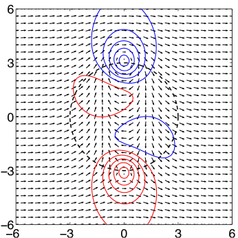
Figure 1: Magnetisation configuration of type I (long VA pair) for vortex-antivortex pair in steady-state rotation around a nano-aperture (delimited by a dashed line). The vector plot shows $(m_{1},m_{2})$ and the contour plot is for the perpendicular magnetisation component. We plot contour levels $m_{3}=\pm 0.1,\pm 0.3,\pm 0.5,\pm 0.7,\pm 0.9$ (red: up, blue: down). Parameters used are $\beta=-0.10,\;h_{\rm ext}=0.40$ and (12). The angular frequency of rotation is $\omega=0.255$.

Varying $h_{\rm ext}$ from larger to smaller values we find configurations similar in form to that shown in Fig. 2 for the value $h_{\rm ext}=0.4$. We label these VA pairs as type II (or short VA pairs). Note that the two VA pairs shown in Figs. 1, 2 are obtained for the same parameter values, but they are different and they have significantly different rotation frequencies.

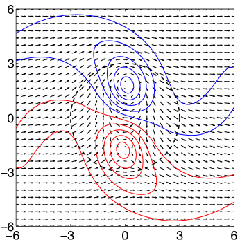
Figure 2: Magnetisation configuration of type II (short VA pair) in steady-state rotation. We plot as in Fig. 1. Parameters used are $\beta=-0.10,\;h_{\rm ext}=0.40$ (the same as in Fig. 1). The angular frequency of rotation is $\omega=0.539$.

Increasing the spin current to $\beta=-0.2$ and choosing large external field values we find still one more kind of VA pairs, shown in Fig. 3 for the value $h_{\rm ext}=0.6$. We label these VA pairs of type III (or wide VA pairs).

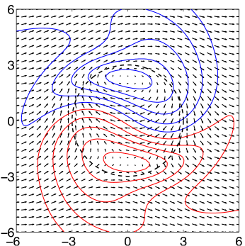
Figure 3: Magnetisation configuration of type III (wide VA pair) in steady-state rotation. We plot as in Fig. 1. Parameters used are $\beta=-0.20,\;h_{\rm ext}=0.60$. The angular frequency of rotation is $\omega=0.820$.

We have explored systematically the range of parameters $0\leq|\beta|\leq 0.7$ and $0\leq h_{\rm ext}\leq 0.7$. We find the three types of VA pairs in steady-state rotation on the $\beta-h_{\rm ext}$ plane as shown in Fig. 4. Each symbol corresponds to a numerical simulation which has successfully converged to a VA pair rotating in a steady-state. Stars correspond to long VA pairs, circles to short pairs and crosses to wide pairs. There are small regions in the parameter space where more than one type of VA pairs has been found. We obtain either one or the other configuration depending on the initial condition used or on the direction of sweeping the parameter space. In a significant word of caution we mention that our simulations do not prove that the calculated states represent exact steady-states. While most of these seem to be exact within our numerical accuracy, in some others we measure small fluctuations. Especially the wide pairs for smaller $h_{\rm ext}$ show fluctuations $\sim 1\%-3\%$ in various quantities calculated numerically.

In the areas in Fig. 4 where no symbols are plotted we have found no steady-state rotating VA pairs. Instead, the simulations give dynamical states which do include a VA dipole in rotation, but the motion is accompanied by a continuous creation and annihilation of more VA pairs with same polarities. We will not refer any further to these dynamical states in the present paper. Simulations and studies of similar states in a related system have been given in Refs. BerkovGorn_PRB2009 ; BerkovGorn_JPD2008 .

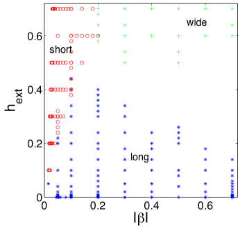
Figure 4: Numerical simulations have given three types of rotating VA pairs. In the $\beta-h_{\rm ext}$ plane we plot blue stars for type I (long) pairs, red circles for type II (short) VA pairs, and green crosses for type III (wide) VA pairs. No steady-states were found in the regions where no symbols are plotted: (a) for very small $\beta$ values and (b) for large $\beta$ and intermediate $h_{\rm ext}$. Other parameters as in Eq. (12).

IV.2 Frequency of rotation

For a more detailed presentation of results we fix the spin-torque parameter $\beta$ and vary the field $h_{\rm ext}$. In Fig. 5 we present the angular frequency $\omega$ of VA pair rotation for three fixed values of the spin-torque and for external field values in the range $0\leq h_{\rm ext}\leq 0.7$. For $\beta=-0.1$ and $0\leq h_{\rm ext}\leq 0.44$ we find long VA pairs and for $0.38\leq h_{\rm ext}\leq 0.7$ we find short VA pairs. The transition between the two kind of VA pairs is not smooth, the magnetic configuration and the angular frequency change significantly. Furthermore, the two types of VA pairs coexist for the range $0.38\leq h_{\rm ext}\leq 0.44$. For $\beta=-0.05$ there is a small gap in the range of $h_{\rm ext}$ where no steady-state rotating VA pairs are found. For $\beta=-0.3$ we have long pairs for small $h_{\rm ext}$, wide pairs for large $h_{\rm ext}$ and no steady states for a range of $h_{\rm ext}$ in-between.

VA pairs are certainly stable also for $h_{\rm ext}=0$ and they are rotating at a nonzero $\omega$. We find $\omega=0.49$ for $\beta=-0.05$ and $\omega=0.31$ for $\beta=-0.1$ and $\omega=0.20$ for $\beta=-0.3$.

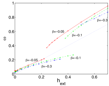
Figure 5: Angular frequency $\omega$ of rotation (absolute value) as a function of external field $h_{\rm ext}$ for three fixed values of the current density $\beta=-0.05$ (solid-red line), $\beta=-0.1$ (dashed-green line), and $\beta=-0.3$ (dashed-dotted-blue line). Stars denote long VA pairs, circles denote short pairs, and crosses denote wide pairs. The frequency $\omega$ goes to a nonzero value for $h_{\rm ext}=0$. There is a jump in the frequency when we change from long to short or wide pairs. For $\beta=-0.1$ two types of VA pairs coexist for a range of $h_{\rm ext}$ values. The dotted line shows $\omega=h_{\rm ext}$ for comparison purposes.

We continue by fixing $h_{\rm ext}=0.1$ and varying $\beta$. In Fig. 6 we present the angular frequency $\omega$ of rotation for three values of $h_{\rm ext}$ and for spin-torque in the range $0\leq|\beta|\leq 0.7$. For $h_{\rm ext}=0.1$ we find long VA pairs for $0.022\leq|\beta|\leq 0.7$ and short VA pairs for $0.016\leq|\beta|\leq 0.21$. The transition between the two kinds of VA pairs is not smooth, and the angular frequency jumps. This becomes completely obvious for $h_{\rm ext}=0.4$ where we have a significant jump to higher frequencies for short VA pairs at $|\beta|\approx 0.1$. For the values $0.08\leq|\beta|\leq 0.1$ both long and short pairs are found. For $h_{\rm ext}=0.7$ we have short VA pairs for smaller $|\beta|$ values and wide pairs for larger values of the spin-torque.

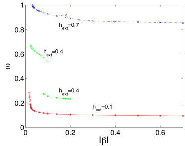
Figure 6: Angular frequency $\omega$ of rotation as a function of spin-torque $\beta$ for three fixed values of the external field $h_{\rm ext}=0.1$ (solid-red line), $h_{\rm ext}=0.4$ (dashed-green line), and $h_{\rm ext}=0.7$ (dashed-dotted-blue line). Stars denote long VA pairs, circles denote short pairs, and crosses denote wide pairs. There is a jump in the frequency when we change from long to short or wide pairs in all case, but it is much more pronounced for $h_{\rm ext}=0.4$. No VA pairs are sustained for very small values of $|\beta|$. The frequency $\omega$ increases sharply for small $\beta$ and is nearly saturated for large spin-torque values.

A quantity of potential interest for experimental work and applications is the distance $d_{\rm VA}$ between vortex and antivortex defined in Eq. (9). Fig. 8 shows $d_{\rm VA}$ as a function of $h_{\rm ext}$ for three values of $\beta$. Larger values of $h_{\rm ext}$ tend to make the VA pair shrink, as $h_{\rm ext}$ favors the ground state. Fig. 7 shows $d_{\rm VA}$ as a function of $\beta$ for three values of external field $h_{\rm ext}$. The main features are that (i) $d_{\rm VA}$ saturates for strong spin torque and (ii) the vortex and antivortex come very close together for small $\beta$ values or for large $h_{\rm ext}$.

VA dipoles are sustained even for quite small values of $\beta$. Smaller $|\beta|$ gives smaller VA pairs and larger $\omega$. For very small values of $\beta$ below a certain threshold (which depends on $h_{\rm ext}$, as can be seen in Fig. 4) the simulations show collapse of any initial configuration to the ground state. An estimation for the maximum possible $\omega$ is given in Sec. IV.3.

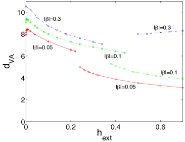
Figure 7: Separation distance between vortex and antivortex defined in Eq. (9) as a function of external field $h_{\rm ext}$ for three fixed values of the current density $\beta=-0.05$ (solid-red line), $\beta=-0.1$ (dashed-green line), and $\beta=-0.3$ (dashed-dotted-blue line). Stars denote long VA pairs, circles denote short VA pairs, and crosses denote wide pairs. The magnetic field favors the ground state so it acts to shrink the VA pairs, i.e., decrease $d_{\rm VA}$. The sharp change for $d_{\rm VA}$ for very small $h_{\rm ext}<0.01$ is discussed in Sec. IV.3.

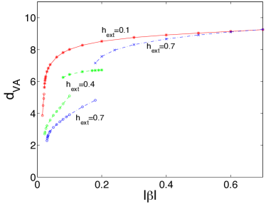
Figure 8: Separation distance between vortex and antivortex defined in Eq. (9) as a function of spin-torque $\beta$ for three fixed values of the external field $h_{\rm ext}=0.1$ (solid-red line), $h_{\rm ext}=0.4$ (dashed-green line), and $h_{\rm ext}=0.7$ (dashed-dotted-blue line). Stars denote long VA pairs, circles denote short VA pairs, and crosses denote wide pairs. For very small $\beta$ no VA pairs are sustained. The vortex and antivortex come closer for small $\beta$, and $d_{\rm VA}$ saturates for large $\beta$.

It appears straightforward to understand the long VA pairs as a combination of a vortex and an antivortex which are well-separated but still interacting. This is in accordance with the overall configuration but also with the detailed features obtained in the simulations. For example, the anisotropy energy of long VA pairs is roughly twice that of a single isolated vortex, i.e., $E_{\rm a}\approx\pi$. The short as well as the wide VA pairs are characterised by the fact that their magnetisation is roughly similar to their angular momentum, i.e., $\mu_{1}\approx\ell$. This is a feature present in two-meron configurations which are solutions of the pure exchange model Gross_NPB1978 ; Komineas_EPL2012 . The short and the wide VA pairs thus appear to be related to two-meron configurations, except that, unlike merons such as in Eq. (21), the VA dipole configuration decays exponentially to the ground state at large distances and is thus well-localised. The wide VA pairs appear to have a large anisotropy energy $E_{\rm a}\approx 20$, which is many times larger than the anisotropy energy of two isolated vortices.

In some cases we can have approximations for $\omega$ directly derived from the virial relation (7). For the case of very small external field the vortex and antivortex are well separated, so we can use the approximation $E_{\rm a}\approx\pi$ and Eq. (9). Then, the virial relation for long VA pairs, in the case $h_{\rm ext}\ll 1$, gives

$$\omega\approx\frac{2}{d_{\rm VA}^{2}}.$$ (13)

For long VA pairs at external fields $h_{\rm ext}>0.1$, we find in simulations $\ell>\mu_{1}$. Therefore, the virial relation (7) indicates an angular frequency $\omega<2/d_{\rm VA}^{2}+h_{\rm ext}$.

Short VA pairs appear for larger external fields. Since $\mu_{1}\approx\ell$ the virial relation gives

$$\omega\approx\frac{E_{\rm a}}{\ell}+h_{\rm ext}.$$ (14)

The first term on the right hand side depends on the precise form of the magnetic configuration. The approximations given before Eq. (13) are not very good any more, however, one could still use them as a rough guide obtaining a contribution $\sim 1/d_{\rm VA}^{2}$ to the angular frequency. Approximation (14) is valid for wide VA pairs, too, for which we also have $\mu_{1}\approx\ell$. These VA pairs have large anisotropy energy $E_{\rm a}\sim 20$ and also larger angular momentum $\ell$. Their angular frequency $\omega$ tend to be similar to that for short VA pairs at similar $h_{\rm ext}$ values as seen in Fig. 6.

IV.3 Asymptotics for large distances

An asymptotic analysis for large distances from the VA pair center is given in Appendix C. The main conclusion is that the behavior of the magnetic configuration as $\rho\to\infty$ is given by a system of Bessel equations. The main features of the solutions depend on the eigenvalues (30), and their asymptotic behavior (31) on the values of $\lambda_{1,2}$ in Eq. (32). The values of these quantities are found provided the angular frequency $\omega$ is known from the simulations.

A case of special interest is $\mu_{1}\geq 0$. This gives $\lambda_{2}=0$ in the case of no damping ($\alpha=0$) via Eq. (32) and thus a non-exponential decay of the magnetic configuration to the uniform state, as described by the Hankel functions $H_{n}$ in Eq. (31). If dissipation is present ($\alpha>0$) then $\lambda_{2}>0$ so we do have exponential decay, but this is slow, so that unusual behavior could be expected.

Let us see the special case of no external field $h_{\rm ext}=0$, for which we have $\mu_{+}\approx\omega^{2}$. Such a positive $\mu_{1}=\mu_{+}$ means a slow decay for the Hankel functions (31). For values of the external field $h_{\rm ext}\sim 0.01$ the numerical data show that the eigenvalue $\mu_{1}=\mu_{+}$ turns negative and thus $\lambda_{2}$ acquires larger values, that is, the decay of the magnetic configuration to the uniform state becomes fast. The described behavior of the eigenvalue $\mu_{1}$ explains the great sensitivity, shown in Fig. 7, of $d_{\rm VA}$ on $h_{\rm ext}$ for very small fields $h_{\rm ext}<0.01$. The angular frequency shown in Fig. 5 is correspondingly very sensitive for small $h_{\rm ext}$, although this is not revealed in the scale of the figure.

Fig. 6 shows faster rotation for smaller $\beta$ at a fixed $h_{\rm ext}$. This is due to the vortex and antivortex getting closer to each other. An increased $\omega$ leads to values for $\mu_{1}=\mu_{+}$ closer to zero according to Eq. (30). We have $\mu_{+}=0$ for angular frequency equal to

$$\omega_{\rm max}=\sqrt{h_{\rm ext}(1+h_{\rm ext})},$$ (15)

and we would thus expect the magnetic configuration to tend to delocalise for larger $\omega$ values ($\omega\gtrsim\omega_{\rm max}$). Indeed, Eq. (15) gives a fair approximation to the numerical results regarding the maximum angular frequency obtained for fixed $h_{\rm ext}\gtrsim 0.1$. Indeed, no rotation faster than in Eq. (15) was obtained in numerical simulations. We conclude that the slow decay of the configuration is responsible for the unsustainability of VA dipoles at small spin torque strength.

An important lesson from the results of the asymptotic analysis is that the rate of energy dissipation for rotating VA pairs may depend greatly on the features of the magnetisation configuration. For example, a delocalised configuration would dissipate energy much faster than a localised configuration. Put it another way, the rate of energy dissipation may not be proportional to the value of the dissipation constant $\alpha$.

V Uniform spin-current

The results of the previous section showed that when the spin-torque is localised under a nano-aperture we have a favorable situation for the stabilisation of a VA pair. In this section we present simulations and show that there are steady-state rotating VA pairs also in the case that the current flows through a large area.

We assume in this section an uniform external field (6) and an uniform spin current polarization (5). We will present results for the parameter values

$$\alpha=0.1,\qquad\beta=-0.05.$$ (16)

Simulations converge to a steady state rotating VA pair for external fields $h_{\rm ext}\leq 0.156$.

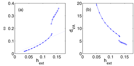
Figure 9: (a) Angular frequency of rotation $\omega$ as a function of the applied field $h_{\rm ext}$. Points connected by lines show numerical results for an uniform spin current and parameter set (16). We have two separate branches of rotating VA pairs. The lower frequency branch (long VA pairs) for $h_{\rm ext}\leq 0.132$ and the upper branch (short VA pairs) for $0.130\leq h_{\rm ext}\leq 0.156$. The dotted line shows $\omega=h_{\rm ext}$ for comparison. (b) The separation distance between vortex and antivortex as a function of applied field $h_{\rm ext}$. The lower frequency branch corresponds to larger VA separation, while the upper frequency branch corresponds to smaller VA separation.

Fig. 9 shows the rotation frequency $\omega$ and the distance $d_{\rm VA}$ between the vortices for parameter set (16) and for the range of values of $h_{\rm ext}$ where a steady state was reached. We find two separate branches of VA pairs. For $h_{\rm ext}\leq 0.132$ we have a branch of low frequencies and large VA pair separation, which correspond to long VA pairs. The branch apparently persists for low values of $h_{\rm ext}$, however, we do not present results for $h_{\rm ext}<0.03$ because the VA separation $d_{\rm VA}$ becomes very large and our numerical results are then not reliable, since the accuracy of the simulations (spatial resolution) for vortices far from the origin is inadequate. A separate branch of short VA pairs with higher frequencies and smaller VA pair separation exists for $0.130\leq h_{\rm ext}\leq 0.156$. For $h_{\rm ext}>0.156$ we find no steady state rotation (the VA pair is annihilated). For a narrow range of external fields, $0.130\leq h_{\rm ext}\leq 0.132$, we have two different steady states and the simulation converges to either a long or a short pair depending on the initial condition.

The Derrick relation (7) is valid here and it is indeed satisfied with an accuracy better than 1% in all our numerical simulations. It provides a guide for the expected frequencies. For short VA pairs we find $\ell\approx\mu_{1}$, so the angular frequency has a significant contribution from the first term on the rhs in Eq. (7) while it is linearly increasing with $h_{\rm ext}$ due to the second term. For long VA pairs we have $\mu_{1}<\ell$, so the main contribution to $\omega$ is due to the second term and it is approximately proportional to $h_{\rm ext}$.

VI Conclusions

Magnetic vortex-antivortex pairs where the vortex and antivortex have opposite polarities have skyrmion number unity, and the configuration can actually be obtained from the usual axially symmetric skyrmions by a transformation. We have studied their dynamics under the influence of spin-polarized current and external magnetic field using the Landau-Lifshitz-Gilbert-Slonczewski equation. Both the polarization of the spin current and the magnetic field are in-plane along the same direction. Their motion is rotational and it is stabilised by the presence of a spin-torque with in-plane polarisation. The field contributes directly to the rotation frequency and also indirectly by bringing the vortex and antivortex closer together so that they interact stronger. The rotational dynamics due to both the interaction between vortex and antivortex and the external field is linked to the skyrmion number.

When an external field is present in the Landau-Lifshitz equation we would typically expect precession of magnetization around the field. In the case of the VA dipole we rather have rotation of magnetization. This surprising result is due to the nonzero skyrmion number of the VA dipole.

The framework developed in the present paper can be applied to spin-transfer oscillators where the magnetization oscillations are produced due to various external probes, i.e., due to external magnetic field and spin-torques with various combinations of polarizations. One possible direction is the oscillations of magnetic bubbles in perpendicular anisotropy materials, in an analogy to precessing droplets HoeferSilva_PRB2010 ; MohseniSani_Science2013 . Also, the effect of perpendicularly oriented polarizers could be analysed MoriyamaFinocchio_PRB2012 .

The derivation of most main results is based on the use of the stereographic projection variable (17). This allows description of a VA dipole configuration via an axially symmetric anzatz, and in special cases it leads to the exact description of the dynamics. Our main results rely upon the form of Eq. (II) but they do not depend on the specific interactions which we included. The present methods can be adapted to study other cases of counterintuitive dynamics of vortices, bubbles and other skyrmions in the presence of spin polarized current.

Aknowledgements

This work was partially supported by the European Union’s FP7-REGPOT-2009-1 project “Archimedes Center for Modeling, Analysis and Computation” (grant agreement n. 245749) and by grant KA3011 of the University of Crete. I gratefully acknowledge discussions with Dimitris Mitsoudis and Dimitris Tsagkarogiannis.

Appendix A Stereographic projection variable

A representation of the magnetisation vector $\bm{m}$ can be given by its stereographic projection on a plane. We define the complex variable

$$X=\frac{m_{2}+im_{3}}{1+m_{1}},$$ (17)

which is the sterographic projection of $\bm{m}$ from the point $\bm{m}=(1,0,0)$. The components of $\bm{m}$ are given as

$$m_{1}=\frac{1-X\overline{X}}{1+X\overline{X}},\quad m_{2}=\frac{X+\overline{X}}{1+X\overline{X}},\quad m_{3}=\frac{1}{i}\,\frac{X-\overline{X}}{1+X\overline{X}},$$ (18)

where $\overline{X}$ is the complex conjugate of $X$. This variable turns out to be particularly useful for studying many properties of the VA dipole.

For the usual conventions adopted in the present paper, we have $\bm{m}(\rho\to\infty)=(1,0,0)\Rightarrow X(\rho\to\infty)=0$ while $\bm{m}(\rho=0)=(-1,0,0)\Rightarrow X(\rho=0)\to\infty$. At the centers of the vortices we have $\bm{m}=(0,0,\pm 1)\Rightarrow X=\pm i$.

The Landau-Lifshitz-Gilbert-Slonczewski equation of motion, when we assume external field (6) and spin polarisation (5), takes the following form

$$\begin{split}(i+\alpha)\,\dot{X}&=\partial_{\mu}\partial_{\mu}X-\frac{2\overline{X}}{1+X\overline{X}}\,\partial_{\mu}X\partial_{\mu}X\\ &-\frac{1}{2}\,\frac{X-\overline{X}}{1+X\overline{X}}\,(1+X^{2})-(h_{\rm ext}+i\beta)\,X,\end{split}$$ (19)

where $\mu=1,2$ and summation is implied.

We can further use the complex position $z=x+iy$ on the $xy$-plane, denote its complex conjugate by ${\bar{z}}$, so we consider $X=X(z,{\bar{z}},t)$. The skyrmion number is given by

$$\mathcal{N}=\frac{1}{4\pi}\int n\,d^{2}x,\qquad n=4\,\frac{|\partial_{z}X|^{2}-|\partial_{\bar{z}}X|^{2}}{(1+X\overline{X})^{2}}.$$ (20)

Of particular interest here is the form

$$X=\frac{\bar{a}}{{\bar{z}}},$$ (21)

where $a$ is a complex constant and $\bar{a}$ its complex conjugate. This represents a skyrmion with $\mathcal{N}=1$ as can be calculated using (20). Configuration (21) consists of two merons at a distance $2|a|$ apart, while each of the merons has core size $|a|$ Gross_NPB1978 . Note that, at $z=\pm ia$ we have $m_{3}=\pm 1$, so the two-meron configuration can also be viewed as a VA dipole where a vortex with negative polarity is centered at $z=-ia$ and an antivortex with positive polarity at $z=ia$. The constant $|a|$ gives the vortex core size and the distance between the vortex and the antivortex is $d_{\rm VA}=2|a|$. More general skyrmion configuration have been studied in Ref. Gross_NPB1978 .

Appendix B A virial relation

Motivated by the steady state rotating solutions of the exchange model, let us assume the existence of similar steady states in the full model (II). More precisely, we assume a configuration rigidly rotating at an angular frequency $\omega$, so we have

$$\dot{\bm{m}}=-\omega\,\epsilon_{\lambda\nu}\,x_{\lambda}\partial_{\nu}\bm{m}.$$ (22)

This is inserted in Eq. (II) to obtain virial (integral) relations. The procedure is developed in Ref. Papanicolaou91 and it is applied for the LLG equation. For an uniform magnetic field (6) and a spin-torque term with polarization (5) a generalisation of this procedure gives a, so-called, Derrick relation Komineas_EPL2012 :

$$\omega \left(\ell+\frac{\alpha}{2}\int\epsilon_{\lambda\nu}\,x_{\lambda}x_{\mu}d_{\mu\nu}\,d^{2}x\right)=$$

$$-\left(E_{\rm a}+h_{\rm ext}\,\mu_{1}+\frac{1}{2}\int x_{\mu}\tau_{\mu}\,d^{2}x\right),$$ (23)

where

$$d_{\mu\nu} \equiv\partial_{\mu}\bm{m}\cdot\partial_{\nu}\bm{m},$$

$$\tau_{\mu} \equiv-\beta(\bm{m}\times\partial_{\mu}\bm{m})\cdot\bm{p}$$ (24)

and all other symbols are explained in the main body of the paper. All the integrals are understood to extend over the whole plane. The Derrick relation (B) is valid for all steady-state rotating solutions.

Appendix C Asymptotics

We are interested in the behavior of the magnetization at large distances from the VA pair as we expect that localisation properties of the configuration could play a significant role in its stability. We look in configuration for which $X(\rho\to\infty)\to 0$, so we linearise (19) while it will be convenient to use polar coordinates $(\rho,\phi)$. We are interested in steady rotational motion so we assume $\dot{X}=-\omega\partial_{\phi}X$. The linearised form of (19), with the latter substitution, is

$$\begin{split}\left(\partial_{\rho}^{2}X+\frac{\partial_{\rho}X}{\rho}+\frac{\partial_{\phi}^{2}X}{\rho^{2}}\right)-\frac{1}{2}\,(X-\overline{X})&\\ -(h_{\rm ext}+i\beta)\,X+\omega(i+\alpha)\,\partial_{\phi}X&=0.\end{split}$$ (25)

We use a Fourier series of the form

$$X(\rho,\phi)=\sum_{n=-\infty}^{\infty}X_{n}(\rho)\,e^{in\phi},$$ (26)

where $X_{n}$ are complex functions of $\rho$. Substituting (26) in (25) we obtain a linear system of differential equations for the $X_{n}$’s. These should satisfy Bessel equation

$$\left(\partial^{2}_{\rho}+\frac{\partial_{\rho}}{\rho}-\frac{n^{2}}{\rho^{2}}\right)X_{n}=-(\mu_{1}+i\mu_{2})X_{n},$$ (27)

where we have introduced a complex eigenvalue $\mu_{1}+i\mu_{2}$. So we write

$$X_{n}(\rho)\sim X_{n}^{0}\;H_{n}\left(\sqrt{\mu_{1}+i\mu_{2}}\,\rho\right),$$ (28)

where $X_{n}^{0}$ are complex constants and $H_{n}$ are Hankel functions Watson ; AbramowitzStegun .

Substituting the form (28) in the system of differential equations for $X_{n}$ we obtain an algebraic system which is closed for every pair of unknowns $X_{n}^{0},X_{-n}^{0}$. The characteristic equation for the system is

$$\begin{vmatrix}-(M_{1}+n\omega)-iM_{2}&\frac{1}{2}\\ \frac{1}{2}&-(M_{1}-n\omega)-iM_{2}\\ \end{vmatrix}=0,$$ (29)

where $M_{1}\equiv\mu_{1}+h_{\rm ext}+q/2$ and $M_{2}\equiv\mu_{2}-n\alpha\omega$. Note that $\beta$ does not appear in this condition as we consider here the case where the spin-torque term is localised around the origin and is therefore zero at large distances. We have

$$\begin{split}&\mu_{1}=\mu_{\pm}\equiv-\left(\frac{1}{2}+h_{\rm ext}\right)\pm\sqrt{\frac{1}{4}+(n\omega)^{2}}\\ &\mu_{2}=n\alpha\omega.\end{split}$$ (30)

We will need to focus on the behavior of the Hankel functions at spatial infinity ($\rho\to\infty$), which is

$$H_{n}(z)\sim\sqrt{\frac{2}{\pi z}}\;e^{\pm i\left(z-\frac{n\pi}{2}-\frac{\pi}{4}\right)},\\$$ (31)

where $z\equiv(\lambda_{1}+i\lambda_{2})\,\rho$ with $\lambda_{1}+i\lambda_{2}=\sqrt{\mu_{1}+i\mu_{2}}$, and we should choose the sign for which the exponent is negative. We require that the decay in Eq. (31) should be slowest for $n=1$ in view of the solutions we study in this paper: these are skyrmion solutions, e.g., as in Eq. (21). So we are interested only in the case $n=1$ in Eq. (30). We have

$$\begin{split}\lambda_{1}&=\frac{1}{2}\,\frac{\alpha\omega}{\lambda_{2}}\\ \lambda_{2}&=\sqrt{\frac{-\mu_{1}+\sqrt{\mu_{1}^{2}+(\alpha\omega)^{2}}}{2}}.\end{split}$$ (32)

More interesting is the case $\mu_{1}=\mu_{+}$ which gives a smaller value for $\lambda_{2}$ and thus slower decay in Eq. (31). In the case $\lambda_{2}=0$ the decay of the configuration to the ground state is non-exponential and then $H_{n}\sim 1/\sqrt{\rho}$. The consequences of such behavior are discussed in Sec. IV.3.

References

- (1) S. E. Russek, W. H. Rippard, T. Cecil, and R. Heindl, Handbook of Nanophysics, Handbook of Nanophysics (CRC Press, Honolulu, USA, 2010), Chap. 38, pp. 1–23.
- (2) D. V. Berkov and N. L. Gorn, Journal of Applied Physics 99, 08Q701 (2006).
- (3) D. V. Berkov and N. L. Gorn, Journal of Physics D: Applied Physics 41, 164013 (2008).
- (4) D. V. Berkov and N. L. Gorn, Phys. Rev. B 80, 064409 (2009).
- (5) G. Finocchio, O. Ozatay, L. Torres, R. A. Buhrman, D. C. Ralph and B. Azzerboni, Phys. Rev. B 78, 174408 (2008).
- (6) V. L. Pokrovskii and G. V. Uimin, JETP Lett. 41, 128 (1985).
- (7) N. Papanicolaou and P. N. Spathis, Nonlinearity 12, 285 (1999).
- (8) S. Komineas, Phys. Rev. Lett. 99, 117202 (2007).
- (9) W. H. Rippard, M. R. Pufall, S. Kaka, S. E. Russek and T. J. Silva, Phys. Rev. Lett. 92, 027201 (2004).
- (10) W. H. Rippard, M. R. Pufall, S. Kaka, T. J. Silva and S. E. Russek, Phys. Rev. B 70, 100406 (2004).
- (11) M. R. Pufall, W. H. Rippard, M. L. Schneider, and S. E. Russek, Phys. Rev. B 75, 140404 (2007).
- (12) S. Komineas, EPL (Europhysics Letters) 98, 57002 (2012).
- (13) J. C. Slonczewski, J. Magn. Magn. Mat. 159, L1 (1996).
- (14) D. Berkov and J. Miltat, J. Magn. Magn. Mat. 320, 1238 (2008).
- (15) R. Rajaraman, Solitons and Instantons (North Holland, Amsterdam, 1982).
- (16) N. Papanicolaou and T. N. Tomaras, Nucl. Phys. B 360, 425 (1991).
- (17) S. Komineas and N. Papanicolaou, Nonlinearity 11, 265 (1998).
- (18) D. J. Gross, Nucl. Phys. B 132, 439 (1978).
- (19) M. A. Hoefer, T. J. Silva, and M. W. Keller, Phys. Rev. B 82, 054432 (2010).
- (20) S. M. Mohseni, S. R. Sani, and J. Persson, T. N. Anh Nguyen, S. Chung, Ye. Pogoryelov, P. K. Muduli, E. Iacocca, A. Eklund, R. K. Dumas, S. Bonetti, A. Deac, M. A. Hoefer, and J. Akerman, Science 339, 1295 (2013).
- (21) T. Moriyama, G. Finocchio, M. Carpentieri, B. Azzerboni, D. C. Ralph, and R. A. Buhrman, Phys. Rev. B 86, 060411 (2012).
- (22) G. N. Watson, A Treatise on the Theory of Bessel Functions (Cambridge University Press, Cambridge, 1922).
- (23) M. Abramowitz and I. A. Stegun, Handbook of Mathematical Functions with Formulas, Graphs, and Mathematical Tables (Dover, New York, 1965).