Efficient Variable-Coefficient Finite-Volume Stokes Solvers

Abstract

We investigate several robust preconditioners for solving the saddle-point linear systems that arise from spatial discretization of unsteady and steady variable-coefficient Stokes equations on a uniform staggered grid. Building on the success of using the classical projection method as a preconditioner for the coupled velocity-pressure system [B. E. Griffith, J. Comp. Phys., 228 (2009), pp. 7565–7595], as well as established techniques for steady and unsteady Stokes flow in the finite-element literature, we construct preconditioners that employ independent generalized Helmholtz and Poisson solvers for the velocity and pressure subproblems. We demonstrate that only a single cycle of a standard geometric multigrid algorithm serves as an effective inexact solver for each of these subproblems. Contrary to traditional wisdom, we find that the Stokes problem can be solved nearly as efficiently as the independent pressure and velocity subproblems, making the overall cost of solving the Stokes system comparable to the cost of classical projection or fractional step methods for incompressible flow, even for steady flow and in the presence of large density and viscosity contrasts. Two of the five preconditioners considered here are found to be robust to GMRES restarts and to increasing problem size, making them suitable for large-scale problems. Our work opens many possibilities for constructing novel unsplit temporal integrators for finite-volume spatial discretizations of the equations of low Mach and incompressible flow dynamics.

Keywords Stokes flow; variable density; variable viscosity; saddle point problems; projection method; preconditioning; GMRES.

1 Introduction

Many numerical methods for solving the time-dependent (unsteady) incompressible [3, 1, 24, 21] or low Mach number [39, 13] equations require the solution of a linear unsteady Stokes flow subproblem. The linear steady Stokes problem is of particular interest for low Reynolds number flows [38, 23] or flow in viscous boundary layers. In this work, we investigate efficient linear solvers for the unsteady and steady Stokes equations in the presence of variable density and viscosity. Specifically, we consider the coupled velocity-pressure Stokes system [45, 19]

$$\left\{\begin{array}[]{ll}{\rho}\bm{u}_{t}+\bm{\nabla}p=\bm{\nabla}\cdot{\bm{\tau}}({\bm{u}})+\bm{f},\\ \bm{\nabla}\cdot\bm{u}=g,\end{array}\right.$$ (1)

where ${\rho\left(\bm{r}\right)}$ is the density, ${\bm{u}\left(\bm{r},t\right)}$ is the velocity, $p\left(\bm{r},t\right)$ is the pressure, $\bm{f}\left(\bm{r},t\right)$ is a force density, and $\bm{\tau}(\bm{u})$ is the viscous stress tensor. A nonzero velocity-divergence $g\left(\bm{r},t\right)$ arises, for example, in low Mach number models because of compositional or temperature variations [39]. The viscous stress $\bm{\tau}(\bm{u})$ is ${\mu}\bm{\nabla}\bm{u}$ for constant viscosity incompressible flow, ${\mu}\left[\bm{\nabla}\bm{u}+(\bm{\nabla}\bm{u})^{T}\right]$ when $g=0$ (incompressible flow), and ${\mu}\left[\bm{\nabla}\bm{u}+(\bm{\nabla}\bm{u})^{T}\right]+({\gamma}-\frac{2}{3}{\mu})(\bm{\nabla}\cdot\bm{u})\bm{I}$ when $g\neq 0$, where ${\mu\left(\bm{r},t\right)}$ is the shear viscosity and ${\gamma\left(\bm{r},t\right)}$ is the bulk viscosity. When the inertial term is neglected, $\rho\bm{u}_{t}=0$, (1) reduces to the time-independent (steady) Stokes equations. In this work we consider periodic boundary conditions and physical boundary conditions that involve velocity only, notably no-slip and free-slip physical boundaries.

Spatial discretization of (1) can be carried out using standard finite-volume or finite-element techniques. Applying the backward Euler scheme to solve the spatially-discretized equations with time step size $\Delta t$, gives the following discrete system for the velocity $\bm{u}^{n+1}$ and the pressure $p^{n+1}$ at the end of time step $n$,

$$\left\{\begin{array}[]{ll}{\rho}\left(\frac{\bm{u}^{n+1}-\bm{u}^{n}}{\Delta t}\right)+\bm{\nabla}p^{n+1}=\bm{\nabla}\cdot{\bm{\tau}}\left({\bm{u}}^{n+1}\right)+\bm{f}^{n+1},\\ \bm{\nabla}\cdot\bm{u}^{n+1}=g^{n+1},\end{array}\right.$$ (2)

where $\bm{f}^{n+1}$ contains external forcing terms such as gravity and any explicitly-handled terms such as, for example, advection. Similar linear systems are obtained with other implicit and semi-implicit temporal discretizations [3, 1, 24]. In the limit $\rho/\Delta t\rightarrow 0$, the system (2) reduces to the steady Stokes equations. Here we will assume that the spatial discretization is stable, more precisely, that the Stokes system (2) is “uniformly solvable” as the spatial discretization becomes finer, i.e., that a suitable measure of the condition number of the Schur complement of (2) remains bounded as the grid spacing $h\rightarrow 0$. In the context of finite-element methods, this is typically implied by the well-known $\inf-\sup$ or Ladyženskaja-Babuška-Brezzi (LBB) condition. Here we employ the classical staggered-grid [29] discretization on a uniform grid, which can be thought of as a rectangular analog of the lowest-order Raviart-Thomas element and is known to be a stable discretization [44, 37]. We expect that it will be relatively straightforward to generalize the preconditioners developed here to recently-developed adaptive mesh staggered schemes [25, 23]. Note, however, that collocated finite-volume discretizations of the Navier-Stokes equations do not provide a stable discretization, which motivates the development of approximate-projection methods [2].

Historically, there have been significant differences in the treatment of (2) in the finite-volume and finite-element literature. In the finite-element literature, there is a long history of numerical methods for solving the Stokes equations, especially in the time-independent (steady) context [45, 19]. By contrast, in the context of high-resolution finite-volume methods, the dominant paradigm has been to use a splitting (fractional-step) or projection method [10, 7] to separate the pressure and velocity updates. In part, this choice has been motivated by the target applications, which are often high Reynolds number, or even inviscid, flows. In the inviscid limit, the splitting error associated with projection methods vanishes, and for sufficiently large Reynolds number flows the time step size dictated by advective stability constraints makes the splitting error relatively small. At the same time, the preference for splitting methods stems, in large part, from the perception that solving the saddle-point problem (2) is much more difficult than solving the pressure and velocity subproblems; to quote the authors of Ref. [7], “Spatially discretized versions of the coupled Eqs. … are cumbersome to solve directly.” In fact, one of the first second-order projection methods [3] was developed by starting with a Crank-Nicolson variant of (2) and then approximating the resulting Stokes system using a velocity-pressure splitting that was motivated by the perceived difficulty in solving the coupled system.

Fractional-step approaches, however, suffer from several significant shortcomings. It is well-known, for example, that the splitting introduces a commutator error that leads to the appearance of spurious or “parasitic” modes [14, 7] in the presence of physical boundaries. Furthermore, it is generally not possible to impose the true boundary conditions of the Stokes system in a fractional-step scheme; instead, "artificial" boundary conditions must be imposed in the velocity and pressure subsystems. This has motivated the construction of methods that approximately solve the Stokes system (2) using block-triangular factorizations [40] similar to those employed here to construct preconditioners for iterative methods that solve (2) exactly. This is crucial at small Reynolds numbers because the splitting error becomes larger as viscous effects become more dominant, and projection or approximate factorization methods do not apply in the steady Stokes regime for problems with physical boundary conditions.

Recognizing these problems, one of us investigated the use of projection-like methods as preconditioners for a Krylov method for solving the coupled system (2) [24]. It was found that, contrary to traditional finite-volume wisdom and in agreement with extensive experience in the finite-element context, the saddle-point problem (2) can be efficiently solved using standard multigrid techniques for the velocity and pressure subproblems, for a broad range of parameters. Here we improve and generalize the preconditioners developed in Ref. [24] to account for variable density and variable viscosity, as well as to robustly handle small or zero Reynolds number (steady) flows. Our primary motivation for this work is the development of semi-implicit integrators for the low Mach number equations of fluctuating hydrodynamics for multicomponent fluid mixtures [13]. For these applications it is important to treat the viscosity implicitly (including the limit of steady Stokes flow [12]) due to the large separation of time scales between momentum and mass diffusion (i.e., large Schmidt number). In order to properly include thermal fluctuations with implicit viscous handling it is also necessary to use a coupled Stokes formulation instead of split (projection method) approaches [46, 11].

The preconditioners we investigate here numerically are drawn from the large finite-element literature on Stokes solvers [4, 5, 18, 19, 17, 30, 31, 33, 34, 35, 38, 36, 45]. We will not attempt to review the extensive finite-element literature on preconditioners for Stokes flow here; instead, we will point out the similarities and differences with prior work for each of the preconditioners that we study. When necessary, we generalize the existing preconditioners to finite Reynolds numbers (unsteady Stokes equations) and to variable density and variable viscosity problems. We investigate several alternative preconditioners that solve the velocity and pressure subproblems in different orders. In the finite-element context, variable-viscosity steady Stokes solvers based on several of the preconditioners we investigate here have been developed by several groups [8, 22], and have already been successfully scaled to massively-parallel architectures and very difficult large-contrast geophysical problems. In the finite-volume context, the work most closely related to our work is Ref. [21], which focuses on steady Stokes flow in the presence of large viscosity contrast (i.e., discontinuities) for geodynamic applications. Notably, both our work and the work presented in Ref. [21] are based on a staggered finite-volume discretization and geometric multigrid solvers.

Our primary contribution in this work is that we investigate in detail the computational performance of a collection of four standard preconditioners over a broad range of parameters in the context of a specific but very efficient (in terms of number of degrees of freedom per grid cell) finite-volume discretization. By carefully designing and optimizing the parameters for all of the key components of the solvers, ranging from the geometric multigrid smoothers to the restart frequency of the GMRES solver, we construct a complete solver that can readily be employed to construct novel unsplit temporal integrators for finite-volume (conservative) spatial discretizations of the equations of low Mach and incompressible flow dynamics. Importantly, these unsplit schemes can use the same building blocks (e.g., geometric multigrid solvers and high-resolution advection techniques) and achieve a similar computational complexity as traditional projection methods, as we will demonstrate in future work.

The preconditioners that we investigate are built using two crucial subsolvers. The first of these is a linear solver for the inviscid problem

$$\left\{\begin{array}[]{ll}{\rho}\left(\frac{\bm{u}^{n+1}-\bm{u}^{n}}{\Delta t}\right)+\bm{\nabla}p^{n+1}=\bm{f}^{n+1},\\ \bm{\nabla}\cdot\bm{u}^{n+1}=g^{n+1},\end{array}\right.$$ (3)

the solution of which requires solving a density-weighted pressure Poisson equation

$$-\Delta t\,\bm{\nabla}\cdot\left(\rho^{-1}\bm{\nabla}p^{n+1}\right)=g^{n+1}-\bm{\nabla}\cdot\left(\bm{u}^{n}+\rho^{-1}\bm{f}^{n+1}\Delta t\right).$$

For the staggered-grid finite-volume discretization we employ here, this Poisson problem can efficiently be solved using standard geometric multigrid techniques [1]. The second subsolver required by the preconditioners is a linear solver for the unconstrained variable-coefficient velocity equation,

$${\rho}\left(\frac{\bm{u}^{n+1}-\bm{u}^{n}}{\Delta t}\right)=\bm{\nabla}\cdot{\bm{\tau}}\left({\bm{u}}^{n+1}\right)+\bm{f}^{n+1}.$$ (4)

Note that both (3) and (4) use the same boundary conditions for velocity as the coupled problem, and that natural boundary conditions are required for the pressure when solving (3) on a staggered grid. For constant viscosity incompressible flow $\bm{\nabla}\cdot{\bm{\tau}}\left({\bm{u}}\right)=\mu\bm{\nabla}^{2}{\bm{u}}$ and therefore (4) is a system of $d$ uncoupled Helmholtz equations, where $d$ is the dimensionality. These can be solved efficiently using standard geometric multigrid techniques. For variable viscosity flows or when $g\neq 0$ the different components of velocity are coupled. Here we develop an effective geometric multigrid method for solving (4) that generalizes the classical red-black coloring smoother for the scalar Poisson equation. Since the solution of either (3) or (4) is itself a costly iterative process, it is crucial that the preconditioners require only approximate subsolvers. More precisely, preconditioning should only require the application of linear operators that are spectrally-equivalent [19] to the exact solution operators for (3) or (4). Here we use one or a few cycles of geometric multigrid as approximate solvers for these subproblems. The preconditioners investigated in this work can be easily generalized to other spatial discretizations and boundary condition types by simply modifying the approximate subsolvers for (3) and (4). For example, boundary conditions that couple pressure and viscous stress can be handled by imposing approximate boundary conditions for the subsolvers. In Ref. [24], at physical boundaries on which normal tractions (normal components of the stress tensor) are prescribed, Neumann conditions are imposed on the normal velocity component when solving (4) and Dirichlet conditions are imposed for the pressure when solving (3). For adaptively-refined meshes [25, 23], multilevel geometric multigrid techniques can be used to solve the pressure and velocity subproblems [1, 25].

The organization of this paper is as follows. In section 2, we introduce several preconditioners based on approximating the inverse of the Schur complement. In Section 3 we specialize to a particular staggered-grid second-order finite-volume discretization and give details of our numerical implementation. In Section 4 we perform a detailed study of the efficiency and robustness of the various preconditioners, and select the optimal values for several algorithmic parameters. Finally, we offer some conclusions in Section 5, and then give several technical derivations in an extensive Appendix.

2 Preconditioners

In this section we present several preconditioners for solving the saddle-point linear system (2) that arises after spatio-temporal discretization of (1). Much of the discussion presented here has already appeared scattered through many diverse works in the literature; for the benefit of the reader we provide a condensed but complete summary of the key derivations. For increased generality, we write this system in the form,

$$\bm{M}\left(\begin{array}[]{c}\bm{x}_{\bm{u}}\\ \bm{x}_{p}\end{array}\right)=\left(\begin{array}[]{cc}\bm{A}&\bm{G}\\ -\bm{D}&\bm{0}\end{array}\right)\left(\begin{array}[]{c}\bm{x}_{\bm{u}}\\ \bm{x}_{p}\end{array}\right)=\left(\begin{array}[]{c}\bm{b}_{\bm{u}}\\ \bm{b}_{p}\end{array}\right),$$ (5)

where $(\bm{x}_{\bm{u}},\,\bm{x}_{p})^{T}$ denote the velocity and pressure degrees of freedom, $(\bm{b}_{\bm{u}},\,\bm{b}_{p})^{T}$ are the velocity and pressure right hand sides, $\bm{D}$ denotes a discrete divergence operator, and $\bm{G}$ is a discrete gradient operator. Note that for the staggered-grid discretization that we describe in Section 3, the gradient and divergence operators are negative adjoints of each other for periodic, no-slip, and free-slip boundary conditions, $\bm{G}=(-\bm{D})^{*}$, where star denotes adjoint, making $\bm{M}=\bm{M}^{\star}$ a self-adjoint matrix. Here the linear velocity operator $\bm{A}=\theta{\bm{\rho}}-\bm{L}_{\bm{\mu}}$ combines inertial and viscous effects, where $\theta$ is a parameter that is zero for steady Stokes flow, and $\theta\sim\Delta t^{-1}$ for unsteady flow. The operator ${\bm{\rho}}$ is a mass density matrix (distinct from the standard finite element mass matrix), such that $\bm{\rho}\bm{x}_{\bm{u}}$ is a spatially-discrete (conserved) momentum field. The viscous operator is denoted with $\bm{L}_{\bm{\mu}}$, with $\bm{L}_{\bm{\mu}}\bm{u}$ being a spatial discretization of $\bm{\nabla}\cdot\bm{\tau}(\bm{u})$.

The saddle-point problem (5) can formally be solved by using the inverse of the Schur complement,

$${\displaystyle\bm{S}^{-1}=\left(-\bm{D}\bm{A}^{-1}\bm{G}\right)^{-1},}$$

to obtain the exact solution for the pressure,

$$\bm{x}_{\bm{p}}=-\bm{S}^{-1}({\bm{D}}\bm{A}^{-1}\bm{b}_{\bm{u}}+\bm{b}_{p}),$$ (6)

and for the velocity degrees of freedom,

$$\bm{x}_{\bm{u}}=\bm{A}^{-1}(\bm{b}_{\bm{u}}-\bm{G}\bm{x}_{p})=\bm{A}^{-1}\bm{b}_{\bm{u}}+\bm{A}^{-1}\bm{G}\bm{S}^{-1}(\bm{D}\bm{A}^{-1}\bm{b}_{\bm{u}}+\bm{b}_{p}).$$ (7)

These formal solutions are not useful in practice because the Schur complement cannot be formed explicitly for large three-dimensional grids, nor inverted efficiently. In Ref. [21], the authors investigate evaluating the action of $\bm{S}^{-1}$ in (6) by an outer Krylov solver, which itself relies on evaluating the action of $\bm{A}^{-1}$ in an inner (nested) Krylov solver. We do not investigate this approach here and instead focus on what the authors of Ref. [21] call the “fully coupled preconditioned approach”, in which an approximation of the Schur complement solution is used to construct an effective preconditioner for a Krylov solver applied to the saddle-point problem (5). The key part in designing preconditioners for (5) is approximating the (inverse of the) Schur complement, specifically, constructing an operator $\mathcal{S}^{-1}$ that is spectrally-equivalent to $\bm{S}^{-1}$ [18].

To motivate the approximation of $\bm{S}^{-1}$, let us consider the case of constant viscosity $\mu_{0}$ and constant density $\rho_{0}$. In this case $\bm{A}=\theta\rho_{0}\bm{I}-\mu_{0}\bm{L}$, where $\bm{I}$ denotes an identity matrix and $\bm{L}$ is a discrete vector Laplacian operator, constructed taking into account the imposed velocity boundary conditions. We then have

$$\bm{S}^{-1}=\left[-\bm{D}\left(\theta\rho_{0}\bm{I}-\mu_{0}\bm{L}\right)^{-1}\bm{G}\right]^{-1}\approx\left[\left(-\bm{D}\bm{G}\right)\left(\theta\rho_{0}\bm{I}-\mu_{0}\bm{L}_{p}\right)^{-1}\right]^{-1}=-\theta\rho_{0}\bm{L}_{p}^{-1}+\mu_{0}\bm{I},$$ (8)

where $\bm{L}_{p}=\bm{D}\bm{G}$ denotes a scalar (pressure) discrete Laplacian operator, and have assumed the commuting property $\bm{L}\bm{G}\approx\bm{G}\bm{L}_{p}$, which is an exact identity for the staggered grid discretization applied to periodic systems. This approximation to the Schur complement inverse has been used in the finite-element context in Ref. [32] and in the finite-volume approach in Ref. [24]; an in-depth discussion of the use of approximate commutators for constructing preconditioners can be found in Ref. [16].

Here we generalize (8) to variable density and viscosity through a simple construction. The basic idea is that the first part of the Schur complement approximation, $\theta\rho_{0}\bm{L}_{p}^{-1}$, corresponds to the inviscid limit. For variable density, this term becomes $\theta\bm{L}_{\bm{\rho}}^{-1}$, where

$${\bm{L}}_{\bm{\rho}}=\bm{D}{\bm{\rho}}^{-1}\bm{G}$$

is a discretization of the density-weighted Poisson operator $\bm{\nabla}\cdot\rho^{-1}\bm{\nabla}$ that also appears in traditional variable-density projection methods [1]. Therefore, for variable-density, constant-viscosity flow, $\bm{\nabla}\cdot\bm{\tau}={\mu}_{0}\bm{\nabla}^{2}\bm{u}$, and we employ the approximation

$$\bm{S}^{-1}\approx\mathcal{S}^{-1}=-\theta\bm{L}_{\bm{\rho}}^{-1}+\mu_{0}\bm{I}.$$ (9)

The term $\mu_{0}\bm{I}$ in (8) is an analogue of the viscous operator $\bm{L}_{\bm{\mu}}$ that acts on pressure-like degrees of freedom instead of velocity-like degrees of freedom. This has to be constructed on a case-by-case basis, and in the constant viscosity setting it corresponds to the viscous pressure-correction term proposed by Brown, Cortez and Minion [7] in the context of second-order projection methods. For incompressible flow, $\bm{\tau}(\bm{u})={\mu}\left[\bm{\nabla}\bm{u}+(\bm{\nabla}\bm{u})^{T}\right]$, the Fourier-space calculation described in Appendix A suggests replacing the term $\mu_{0}\bm{I}$ with $2{\bm{\mu}}$, where ${\bm{\mu}}$ is a diagonal matrix of viscosities corresponding to each pressure degree of freedom. This gives the Schur complement inverse approximation

$$\bm{S}^{-1}\approx\mathcal{S}^{-1}=-\theta{\bm{L}}_{\bm{\rho}}^{-1}+2{\bm{\mu}},$$ (10)

which is called the “local viscosity” preconditioner in Ref. [21]. Note however that the prefactor of two suggested by the analysis in Appendix A is not included in Eq. (36) in Ref. [21]. When bulk viscosity is included, $\bm{\tau}(\bm{u})={\mu}\left[\bm{\nabla}\bm{u}+(\bm{\nabla}\bm{u})^{T}\right]+({\gamma}-\frac{2}{3}{\mu}(\bm{\nabla}\cdot\bm{u}))\bm{I}$, we take

$${\displaystyle\bm{S}^{-1}\approx\mathcal{S}^{-1}=-\theta\bm{L}_{\bm{\rho}}^{-1}+\left({\bm{\gamma}}+\frac{4}{3}{\bm{\mu}}\right),}$$ (11)

where ${\bm{\gamma}}$ is the diagonal matrix of bulk viscosities. As we demonstrate in Appendix A, these approximations are exact for periodic systems if the density and viscosity are constant. In all other cases they are approximations that are expected to be good in regions far from boundaries where the coefficients do not vary significantly. Our numerical experiments support this intuition.

We have investigated the alternative approximations

$$\bm{S}^{-1}\approx-\theta{\bm{L}}_{\bm{\rho}}^{-1}-\bm{L}_{\bm{\rho}}^{-1}\bm{D}{\bm{\rho}}^{-1}\bm{L}_{\bm{\mu}}{\bm{\rho}}^{-1}\bm{G}\bm{L}_{\bm{\rho}}^{-1},$$ (12)

as well as

$$\bm{S}^{-1}\approx-\theta{\bm{L}}_{\bm{\rho}}^{-1}-\bm{L}_{p}^{-1}\left(\bm{D}\bm{L}_{\bm{\mu}}\bm{G}\right)\bm{L}_{p}^{-1},$$

which is similar to the so-called BFBt preconditioner of Elman [18] in the steady-state case, and which is also investigated in Ref. [21]. These approximations utilize the velocity boundary conditions since they involve the viscous operator $\bm{L}_{\bm{\mu}}$, unlike the pressure-space viscous operator in (10) which does not make use of the velocity boundary conditions. We have observed similar behavior for the more expensive approximation (12) as with the simpler and significantly more efficient approximation (10). We therefore do not investigate BFBt-type preconditioners in this work.

As explained in Appendix B, the spectrum of the preconditioned operators for the preconditioners we consider next is determined by the spectrum of $\mathcal{S}^{-1}\bm{S}$. In that appendix, we demonstrate with a combination of analytical techniques and numerical computation that this operator has a very clustered spectrum even in the presence of non-trivial boundary conditions and large variations in viscosity.

2.1 Projection Preconditioner

In the first preconditioner we consider, which we will denote with $\bm{P}_{1}$, we use one step of the classical projection method [10, 3, 24] as a preconditioner. In $\bm{P}_{1}$, we use (6) to estimate the pressure, and make a commuting assumption in (7),

$$\bm{A}^{-1}\bm{G}\bm{S}^{-1}=\bm{A}^{-1}\bm{G}(-\bm{D}\bm{A}^{-1}\bm{G})^{-1}\approx-\bm{A}^{-1}\bm{A}{\bm{\rho}}^{-1}\bm{G}\bm{L}_{\bm{\rho}}^{-1}=-{\bm{\rho}}^{-1}\bm{G}\bm{L}_{\bm{\rho}}^{-1},$$

which gives the velocity estimate

$$\bm{x}_{\bm{u}}\approx\bm{A}^{-1}\bm{b}_{\bm{u}}-{\bm{\rho}}^{-1}\bm{G}\bm{L}_{\bm{\rho}}^{-1}(\bm{D}\bm{A}^{-1}\bm{b}_{\bm{u}}+\bm{b}_{p}).$$ (13)

Note that this velocity estimate (13) satisfies the divergence condition exactly, $\bm{D}\bm{x}_{\bm{u}}=-\bm{b}_{p}$. More precisely, $\bm{x}_{\bm{u}}$ is the $L_{2}$ projection of the unconstrained velocity estimate $\bm{A}^{-1}\bm{b}_{\bm{u}}$ onto the divergence constraint.

In practical implementation, the exact subproblem solvers need to be replaced by approximations. Specifically, ${\bm{A}}^{-1}$ is approximated by the inexact velocity solver $\widetilde{\bm{A}}^{-1}$, $\bm{L}_{\bm{\rho}}^{-1}$ is implemented by the approximate pressure Poisson solver $\widetilde{\bm{L}}_{\bm{\rho}}^{-1}$, and $\bm{S}^{-1}$ is replaced by $\widetilde{\mathcal{S}}^{-1}$, which is an approximation to the approximate Schur complement inverse $\mathcal{S}^{-1}$ given by (10) for incompressible flow. In summary, for the variable-coefficient Stokes problem, the projection preconditioner $\bm{P}_{1}$ is defined by the block factorization

$$\bm{P}_{1}^{-1}=\left(\begin{array}[]{cc}\bm{I}&{\bm{\rho}}^{-1}\bm{G}\widetilde{\bm{L}}_{\bm{\rho}}^{-1}\\ \bm{0}&\widetilde{\mathcal{S}}^{-1}\end{array}\right)\left(\begin{array}[]{cc}\bm{I}&\bm{0}\\ -\bm{D}&-\bm{I}\end{array}\right)\left(\begin{array}[]{cc}\widetilde{\bm{A}}^{-1}&\bm{0}\\ \bm{0}&\bm{I}\end{array}\right).$$ (14)

This factorization clearly shows the main steps in the application of the preconditioner. First, a velocity subproblem is solved inexactly (right-most block) to compute $\bm{x}_{\bm{u}}^{*}=\widetilde{\bm{A}}^{-1}\bm{b}_{\bm{u}}$. Second, $\bm{b}_{c}={\bm{D}}\bm{x}_{\bm{u}}^{*}+\bm{b}_{p}$ is computed (middle block). Third, a Poisson problem is solved approximately to compute $\widetilde{\bm{L}}_{\bm{\rho}}^{-1}\bm{b}_{c}$ and, lastly, the pressure and velocity estimates are evaluated (first block). For constant-coefficient periodic problems with exact subsolvers, the projection preconditioner is an exact solver for the coupled Stokes equations since both (8) and (13) are exact.

For the constant viscosity and density Stokes problem, a projection preconditioner very similar to $\bm{P}_{1}$ was first proposed by one of us in Ref. [24]. In this work we generalize the projection preconditioner to the case of variable viscosity and density. Even in the constant-coefficient case, there is a small but important difference between $\bm{P}_{1}$ and the previous projection preconditioner in Ref. [24], which uses the following approximation of the Schur complement inverse,

$$\bm{S}^{-1}\approx\widetilde{\mathcal{S}}^{-1}=-\left(\theta\rho_{0}\bm{I}-\mu_{0}\bm{L}_{p}\right)\widetilde{\bm{L}}_{p}^{-1},$$

rather than the approximation (9) used here, $\widetilde{\mathcal{S}}^{-1}=-\theta\rho_{0}\widetilde{\bm{L}}_{p}^{-1}+\mu_{0}\bm{I}$, which we have found to give a slightly more efficient solver. The two approximations are identical when exact Poisson solvers are used, $\widetilde{\bm{L}}_{p}^{-1}=\bm{L}_{p}^{-1}$, but not when an approximate solver is employed.

2.2 Lower Triangular Preconditioner

For our second preconditioner, which we denote with $\bm{P}_{2}$, we use (6) for the pressure estimate, but the velocity estimate takes the simpler form

$$\bm{x}_{\bm{u}}\approx{\bm{A}}^{-1}\bm{b}_{\bm{u}},$$ (15)

which is obtained by discarding the second part in (7). If we further approximate the matrix inverses with inexact solves, namely, replacing ${\bm{A}}^{-1}$ by $\widetilde{\bm{A}}^{-1}$, $\bm{L}_{\bm{\rho}}^{-1}$ by $\widetilde{\bm{L}}_{\bm{\rho}}^{-1}$, and $\bm{S}^{-1}$ by $\widetilde{\mathcal{S}}^{-1}$, the second preconditioner is given by the block factorization

$$\bm{P}_{2}^{-1}=\left(\begin{array}[]{cc}\bm{I}&\bm{0}\\ \bm{0}&-\widetilde{\mathcal{S}}^{-1}\end{array}\right)\left(\begin{array}[]{cc}\bm{I}&\bm{0}\\ \bm{D}&\bm{I}\end{array}\right)\left(\begin{array}[]{cc}\widetilde{\bm{A}}^{-1}&\bm{0}\\ \bm{0}&\bm{I}\end{array}\right).$$ (16)

By combing all the terms in the right hand side of (16), we see that $\bm{P}_{2}$ is actually an approximation of the inverse of the lower triangular preconditioner previously studied by several other groups [9, 30, 31, 33, 34],

$$\bm{P}_{2}^{-1}\approx\left(\begin{array}[]{cc}\bm{A}&\bm{0}\\ -\bm{D}&-\bm{S}\end{array}\right)^{-1}.$$ (17)

Notice that for steady Stokes flow, $\theta=0$, the application of $\bm{P}_{2}^{-1}$ does not require any pressure Poisson solvers, unlike the projection preconditioner. Therefore, a single application of $\bm{P}_{2}^{-1}$ can be significantly less expensive computationally than an application of $\bm{P}_{1}^{-1}$. For unsteady flows $\bm{P}_{1}$ and $\bm{P}_{2}$ involve nearly the same operations and applying them has similar computational cost.

2.3 Upper Triangular Preconditioner

Alternatively, one can assume $\bm{D}\bm{A}^{-1}\bm{b}_{\bm{u}}\approx 0$ to obtain $\bm{x}_{p}=-\bm{S}^{-1}\bm{b}_{p}$ and

$${\displaystyle\bm{x}_{\bm{u}}={\bm{A}}^{-1}(\bm{b}_{\bm{u}}+\bm{G}\bm{S}^{-1}\bm{b}_{p}).}$$

Replacing the exact solvers with inexact solvers, we obtain our third preconditioner in block factorization form,

$$\bm{P}_{3}^{-1}=\left(\begin{array}[]{cc}\widetilde{\bm{A}}^{-1}&\bm{0}\\ \bm{0}&\bm{I}\end{array}\right)\left(\begin{array}[]{cc}\bm{I}&-\bm{G}\\ \bm{0}&\bm{I}\end{array}\right)\left(\begin{array}[]{cc}\bm{I}&\bm{0}\\ \bm{0}&-\widetilde{\mathcal{S}}^{-1}\end{array}\right),$$ (18)

which is exactly the same as the “fully coupled” approach with the “local viscosity” preconditioner studied in Ref. [21] and also the block-triangular preconditioner of Ref. [22], generalized here to time-dependent problems. If we combine all the terms in the right hand side of (18), then we see that $\bm{P}_{3}$ is actually an approximation of the inverse of the upper triangular preconditioner [9, 30, 31, 33, 34],

$$\bm{P}_{3}^{-1}\approx\left(\begin{array}[]{cc}\bm{A}&\bm{G}\\ \bm{0}&-\bm{S}\end{array}\right)^{-1}.$$ (19)

The computational cost of applying $\bm{P}_{3}^{-1}$ is very similar to that of applying $\bm{P}_{2}^{-1}$.

2.4 Other preconditioners

In addition to the three main preconditioners (projection, lower and upper triangular) we study here, we have investigated some other preconditioners. The simplest Schur-complement based preconditioner one can construct is the block diagonal preconditioner [9, 31, 33, 34]

$$\bm{P}_{4}^{-1}=\left(\begin{array}[]{cc}\widetilde{\bm{A}}^{-1}&\bm{0}\\ \bm{0}&-\widetilde{\mathcal{S}}^{-1}\end{array}\right).$$ (20)

This preconditioner has the lowest computational cost of all the preconditioners per Krylov iteration, but it also yields the poorest approximation to the exact solution (6,7). Note, however, that the use of a diagonal preconditioner can make the preconditioned operator symmetric and thus allow for the use of more efficient (short-recurrence) Krylov solvers such as MINRES. This is exploited in Ref. [8] to construct a robust and highly-scalable finite-element discretization of the variable-viscosity steady Stokes equations, using a single cycle of algebraic multigrid for a Laplacian approximation to $\bm{A}$ as an approximate velocity solver.

In Appendix B, we show that $\bm{P}_{1}$, $\bm{P}_{2}$ and $\bm{P}_{3}$ all give the same spectrum for the preconditioned linear operator. It is also well-known that $\bm{P}_{1}$, $\bm{P}_{2}$, $\bm{P}_{3}$, and $\bm{P}_{4}$ are all spectrally-equivalent if exact solvers are used [19]. Furthermore, if an exact Schur complement inverse is employed, it can be shown for $\bm{P}_{2}$, $\bm{P}_{3}$, and $\bm{P}_{4}$ that any Krylov subspace iterative method with a Galerkin property will require only a small number of iterations (two or three) to converge to the exact answer [35].

As an alternative approximation to (6,7) that is more accurate than the previous approximations, we consider a fifth preconditioner closely-related to the Uzawa method, denoted by $\bm{P}_{5}$. The action of the inverse of this preconditioner $\bm{P}_{5}^{-1}$ cannot easily be written in block-factorization form so we present in the form of pseudo-code:

1. Solve for $\bm{x}_{\bm{u}}^{*}={\widetilde{\bm{A}}}^{-1}\bm{b}_{\bm{u}}$ using multigrid with initial guess $\bm{0}$.

2. Estimate pressure as $\bm{x}_{p}\approx-\widetilde{\mathcal{S}}^{-1}(\bm{D}\bm{x}_{\bm{u}}^{*}+\bm{b}_{p})$.

3. Estimate velocity as $\bm{x}_{\bm{u}}\approx\widetilde{\bm{A}}^{-1}(\bm{b}_{\bm{u}}-\bm{G}\bm{x}_{p})$ using a multigrid solver, starting with $\bm{x}_{\bm{u}}^{*}$ as an initial guess.

If exact solvers are employed the only approximation made in $\bm{P}_{5}$ is the approximation $\bm{S}^{-1}\approx\widetilde{\mathcal{S}}^{-1}$, and as such we expect it to be the best approximation to $\bm{M}^{-1}$. It is, however, also the most expensive of the five preconditioners because it involves two applications of $\widetilde{\bm{A}}^{-1}$. Our goal will be to investigate how well these preconditioners perform in practice with inexact subsolvers.

3 Numerical Implementation

In this section we specialize the relatively general preconditioners from the previous section to a specific second-order conservative finite-volume discretization of the time-dependent Stokes equations on a uniform rectangular grid. We do not discuss here the inclusion of advection in the full Navier-Stokes equations. Schemes that handle advection explicitly using a non-dissipative spatial discretization are described in detail in Refs. [46, 13], and Ref. [24] describes a particular higher-order upwind scheme for uniform staggered-grids.

3.1 Staggered-grid Discretization

For our numerical investigations of the various preconditioners we employ the well-known staggered-grid or MAC discretization of the Stokes equations [29, 28]. This is a conservative discretization that is uniformly div-stable [44, 37]. The scheme defines the degree of freedoms at staggered locations. Specifically, scalar variables including pressure and density are defined at cell centers, while components of vector variables including velocity components are defined at the corresponding faces of the grid [24, 46]. For illustration, we assume that the domain $\Omega$ is rectangular and there are $n_{x}$ cells along the $x$ direction and $n_{y}$ cells along the $y$ direction, with periodic, no-slip (e.g., $\bm{u}=0$ along a boundary) or free-slip (e.g., $v=0$ and $\partial u/\partial y=0$ along the south boundary) boundary conditions specified at each of the domain boundaries. For simplicity, we further assume that the grid spacing along the different directions is constant, $h_{x}=h_{y}=h$.

The divergence of ${\bm{u}}=(u,v)^{T}$ is approximated at cell centers by $\bm{D}{\bm{u}}=D^{x}u+D^{y}v$ with

$$(D^{x}u)_{i,j}=h^{-1}\left(u_{i+\mathchoice{\kern 0.0pt\raise 1.50694pt\hbox{\sevenrm1}\kern-1.04996pt/\kern-1.04996pt\lower 0.75346pt\hbox{\sevenrm2}}{\kern 0.0pt\raise 1.50694pt\hbox{\sevenrm1}\kern-1.04996pt/\kern-1.04996pt\lower 0.75346pt\hbox{\sevenrm2}}{\kern 0.0pt\raise 1.50694pt\hbox{\fiverm1}\kern-1.39998pt/\kern-1.04996pt\lower 0.75346pt\hbox{\fiverm2}}{1\!/2},j}-u_{i-\mathchoice{\kern 0.0pt\raise 1.50694pt\hbox{\sevenrm1}\kern-1.04996pt/\kern-1.04996pt\lower 0.75346pt\hbox{\sevenrm2}}{\kern 0.0pt\raise 1.50694pt\hbox{\sevenrm1}\kern-1.04996pt/\kern-1.04996pt\lower 0.75346pt\hbox{\sevenrm2}}{\kern 0.0pt\raise 1.50694pt\hbox{\fiverm1}\kern-1.39998pt/\kern-1.04996pt\lower 0.75346pt\hbox{\fiverm2}}{1\!/2},j}\right),\quad\quad(D^{y}v)_{i,j}=h^{-1}\left(v_{i,j+\mathchoice{\kern 0.0pt\raise 1.50694pt\hbox{\sevenrm1}\kern-1.04996pt/\kern-1.04996pt\lower 0.75346pt\hbox{\sevenrm2}}{\kern 0.0pt\raise 1.50694pt\hbox{\sevenrm1}\kern-1.04996pt/\kern-1.04996pt\lower 0.75346pt\hbox{\sevenrm2}}{\kern 0.0pt\raise 1.50694pt\hbox{\fiverm1}\kern-1.39998pt/\kern-1.04996pt\lower 0.75346pt\hbox{\fiverm2}}{1\!/2}}-v_{i,j-\mathchoice{\kern 0.0pt\raise 1.50694pt\hbox{\sevenrm1}\kern-1.04996pt/\kern-1.04996pt\lower 0.75346pt\hbox{\sevenrm2}}{\kern 0.0pt\raise 1.50694pt\hbox{\sevenrm1}\kern-1.04996pt/\kern-1.04996pt\lower 0.75346pt\hbox{\sevenrm2}}{\kern 0.0pt\raise 1.50694pt\hbox{\fiverm1}\kern-1.39998pt/\kern-1.04996pt\lower 0.75346pt\hbox{\fiverm2}}{1\!/2}}\right).$$

The gradient of $p$ is approximated at the $x$ and $y$ edges of the grid cells (faces in three dimensions) by $\bm{G}p=(G^{x}p,\,G^{y}p)^{T}$ with

$$(G^{x}p)_{i-\mathchoice{\kern 0.0pt\raise 1.50694pt\hbox{\sevenrm1}\kern-1.04996pt/\kern-1.04996pt\lower 0.75346pt\hbox{\sevenrm2}}{\kern 0.0pt\raise 1.50694pt\hbox{\sevenrm1}\kern-1.04996pt/\kern-1.04996pt\lower 0.75346pt\hbox{\sevenrm2}}{\kern 0.0pt\raise 1.50694pt\hbox{\fiverm1}\kern-1.39998pt/\kern-1.04996pt\lower 0.75346pt\hbox{\fiverm2}}{1\!/2},j}=h^{-1}\left(p_{i,j}-p_{i-1,j}\right),\quad\quad(G^{y}p)_{i,j-\mathchoice{\kern 0.0pt\raise 1.50694pt\hbox{\sevenrm1}\kern-1.04996pt/\kern-1.04996pt\lower 0.75346pt\hbox{\sevenrm2}}{\kern 0.0pt\raise 1.50694pt\hbox{\sevenrm1}\kern-1.04996pt/\kern-1.04996pt\lower 0.75346pt\hbox{\sevenrm2}}{\kern 0.0pt\raise 1.50694pt\hbox{\fiverm1}\kern-1.39998pt/\kern-1.04996pt\lower 0.75346pt\hbox{\fiverm2}}{1\!/2}}=h^{-1}\left(p_{i,j}-p_{i,j-1}\right).$$

For periodic domains or where a homogeneous Dirichlet condition is specified for the normal component of velocity at physical boundaries, the staggered discretization satisfies $\bm{D}=-\bm{G}^{*}$. Note that $\bm{D}\bm{G}=\bm{L}_{p}$, where $\bm{L}_{p}$ is the standard (five-point in two dimensions, seven-point in three dimensions) centered finite difference Laplacian.

For constant viscosity, the finite difference approximation to the vector Laplacian $\bm{\nabla}^{2}{\bm{u}}$ is denoted as $\bm{L}{\bm{u}}=(L^{x}u,\,L^{y}v)$. In the interior of the domain, $\bm{\nabla}^{2}u$ is discretized using the standard five-point discrete Laplacian. In the presence of physical boundaries, $L^{x}u$ is defined at all interior edges/faces where $u$ are defined, and $L^{y}v$ is defined at all interior edges/faces where $v$ are defined. The finite-difference stencils for tangential velocities next to no-slip and free-slip boundaries are modified to account for the boundary conditions, as described in Refs. [24, 46]. Note that for constant viscosity, if one uses the Laplacian form of the viscous term, the different components of velocity are uncoupled.

When the viscosity is not a constant, the strain tensor form of the viscous term is needed, for which

$$\bm{L}_{\bm{\mu}}\bm{u}=\bm{\nabla}\cdot\bm{\tau}(\bm{u})={\displaystyle\left[\begin{array}[]{l}2\frac{\partial}{\partial x}\left({\mu}\frac{\partial u}{\partial x}\right)+\frac{\partial}{\partial y}\left({\mu}\frac{\partial u}{\partial y}+{\mu}\frac{\partial v}{\partial x}\right)\\ 2\frac{\partial}{\partial y}\left({\mu}\frac{\partial v}{\partial y}\right)+\frac{\partial}{\partial x}\left({\mu}\frac{\partial v}{\partial x}+{\mu}\frac{\partial u}{\partial y}\right)\end{array}\right].}$$ (21)

The discretization of $\bm{\nabla}\cdot\bm{\tau}(\bm{u})$ is constructed using standard (staggered) centered second-order differences to give the discrete viscous operator $\bm{L}_{\bm{\mu}}$. Note that even for constant viscosity, there is coupling between the velocity components in (21). For the staggered discretization that we employ here, it can be shown that for constant viscosity $\mu_{0}$, the viscous operator degenerates to a Laplacian, $\bm{L}_{\bm{\mu}}\bm{u}=\mu_{0}\bm{L}\bm{u}$, if $\bm{D}{\bm{u}}=0$. That is, for constant viscosity incompressible flow the solution of the Stokes system is not affected by the choice of the form of the viscous term (By contrast, in fractional step methods, the unprojected velocity and therefore the projected velocity is affected by this choice). However, the Stokes solver is in general affected by the choice of the viscous term, even for constant viscosity. As described in Ref. [13], centered differences for the viscous fluxes that require values outside of the physical domain are replaced by one-sided differences that only use values from the interior cell bordering the boundary and boundary values. The tangential momentum flux is set to zero for any faces of the corresponding control volume that lie on a free-slip boundary, and values in cells outside of the physical domain are never required. The overall discretization is spatially globally second-order accurate.

We build the discrete velocity operator $\bm{A}=\theta{\bm{\rho}}-\bm{L}_{\bm{\mu}}$ from the above centered finite-difference operators. We assume that the density $\rho$ is specified at the cell centers. The density matrix ${\bm{\rho}}$ is constructed by defining the discrete momentum density $\rho{\bm{u}}$ at the cell faces, where the corresponding velocity components are defined. Here we follow Ref. [13] and average the density from cell centers to cell faces,

$$({\bm{\rho}}{\bm{u}})_{i+\mathchoice{\kern 0.0pt\raise 1.50694pt\hbox{\sevenrm1}\kern-1.04996pt/\kern-1.04996pt\lower 0.75346pt\hbox{\sevenrm2}}{\kern 0.0pt\raise 1.50694pt\hbox{\sevenrm1}\kern-1.04996pt/\kern-1.04996pt\lower 0.75346pt\hbox{\sevenrm2}}{\kern 0.0pt\raise 1.50694pt\hbox{\fiverm1}\kern-1.39998pt/\kern-1.04996pt\lower 0.75346pt\hbox{\fiverm2}}{1\!/2},j}=\left(\frac{\rho_{i,j}+\rho_{i+1,j}}{2}\right)u_{i+\mathchoice{\kern 0.0pt\raise 1.50694pt\hbox{\sevenrm1}\kern-1.04996pt/\kern-1.04996pt\lower 0.75346pt\hbox{\sevenrm2}}{\kern 0.0pt\raise 1.50694pt\hbox{\sevenrm1}\kern-1.04996pt/\kern-1.04996pt\lower 0.75346pt\hbox{\sevenrm2}}{\kern 0.0pt\raise 1.50694pt\hbox{\fiverm1}\kern-1.39998pt/\kern-1.04996pt\lower 0.75346pt\hbox{\fiverm2}}{1\!/2},j}\quad\mbox{and}\quad({\bm{\rho}}{\bm{u}})_{i,j+\mathchoice{\kern 0.0pt\raise 1.50694pt\hbox{\sevenrm1}\kern-1.04996pt/\kern-1.04996pt\lower 0.75346pt\hbox{\sevenrm2}}{\kern 0.0pt\raise 1.50694pt\hbox{\sevenrm1}\kern-1.04996pt/\kern-1.04996pt\lower 0.75346pt\hbox{\sevenrm2}}{\kern 0.0pt\raise 1.50694pt\hbox{\fiverm1}\kern-1.39998pt/\kern-1.04996pt\lower 0.75346pt\hbox{\fiverm2}}{1\!/2}}=\left(\frac{\rho_{i,j}+\rho_{i,j+1}}{2}\right)v_{i,j+\mathchoice{\kern 0.0pt\raise 1.50694pt\hbox{\sevenrm1}\kern-1.04996pt/\kern-1.04996pt\lower 0.75346pt\hbox{\sevenrm2}}{\kern 0.0pt\raise 1.50694pt\hbox{\sevenrm1}\kern-1.04996pt/\kern-1.04996pt\lower 0.75346pt\hbox{\sevenrm2}}{\kern 0.0pt\raise 1.50694pt\hbox{\fiverm1}\kern-1.39998pt/\kern-1.04996pt\lower 0.75346pt\hbox{\fiverm2}}{1\!/2}},$$

giving a diagonal density matrix ${\bm{\rho}}$ with the interpolated face-centered densities along the diagonal. We will assume here that the shear ${\bm{\mu}}$ and bulk ${\bm{\gamma}}$ viscosities are specified at the cell centers; typically they are an explicit function of other scalar variables such as density, temperature, and/or composition. The matrices ${\bm{\mu}}$ and ${\bm{\gamma}}$ that appear in the approximation to the Schur complement [e.g. Eq. (11)] are diagonal matrices containing the cell-centered values of the shear and bulk viscosities. The discretization of the viscous operator $\bm{L}_{\bm{\mu}}$ requires a shear viscosity at both cell-centers and nodes (edges in three dimensions). The value of ${\mu}$ at a node is set to be the average of the four neighboring cell-centered values [13]. Note that the Schur complement approximation uses only the cell-centered and not the node-centered viscosities.

3.2 Krylov Solver

Having defined the discrete operators appearing in the Stokes system (5), we briefly discuss some issues that arise when solving this saddle-point problem using an iterative Krylov solver. The basic operation required by the Krylov solver is computing $\bm{M}\bm{x}$, which amounts to a straightforward direct evaluation of the appropriate finite-difference stencils at every interior face and every cell center in the computational grid.

Application of any of the preconditioners requires implementing approximate solvers for the pressure and velocity subproblems (i.e., application of $\widetilde{\bm{L}}_{\bm{\rho}}^{-1}$and $\widetilde{\bm{A}}^{-1}$). Here we employ geometric multigrid techniques to implement these solvers. For the cell-centered pressure solver we use standard variable-coefficient Poisson multigrid solvers [1]. For the face-centered velocity solver we develop a vector variant of a standard scalar Helmholtz solver based on a generalized red-black Gauss-Seidel smoother. The details of the multigrid algorithms are given in Appendix C. Our implementation is based on the Fortran version of the BoxLib library [41].

Note that because the preconditioners in Krylov methods are applied to a residual-correction system, zero is an appropriate initial guess for the multigrid subsolvers. Note also that for certain choices of boundary conditions the pressure subproblem has a null space of constant vectors. Similarly, for periodic steady-state problems the velocity equation has a ($d$-dimensional) null-space of all constant velocity fields. In these cases some care is needed in the implementation of the preconditioners to ensure that the null-space is handled consistently and the mean pressure and momentum are kept constant at certain prescribed values (e.g., zero). When non-homogeneous velocity boundary conditions are specified, the viscous operator is an affine operator because the viscous stencils near the boundary use the specified boundary values. Because Krylov solvers require a linear rather than an affine operator, we apply the Krylov solver to the homogeneous form of the Stokes problem by subtracting the boundary terms in a pre-processing step.

Here we employ left preconditioning and apply the iterative solver to the preconditioned system $\bm{P}^{-1}\bm{M}\bm{x}=\bm{P}^{-1}\bm{b}$. The convergence criterion for the Krylov solver is therefore most naturally expressed in terms of either the absolute or relative reduction in the magnitude of the preconditioned residual $r_{P}=\left\|\bm{P}^{-1}\left(\bm{M}\bm{x}-\bm{b}\right)\right\|_{2}$. A more robust alternative is to base convergence criteria on the value of the unpreconditioned (true) residual $r=\left\|\bm{M}\bm{x}-\bm{b}\right\|_{2}$. For the problems studies here we observe $r$ and $r_{P}$ to exhibit similar convergence for well-scaled problems.

3.3 Rescaling of the Linear System

Another issue that arises when solving saddle-point problems is that of scaling of the system to minimize the loss of floating point precision occurs when adding the different terms. This is particularly important when the equations are solved in dimensional form (with physical units), but can also be important even when the equations are non-dimensionalized. We consider re-scaling the velocity equations by some constant $c$ and re-scaling the pressure unknowns by the same factor, to obtain the rescaled system

$$\left(\begin{array}[]{cc}c\bm{A}&\bm{G}\\ -\bm{D}&\bm{0}\end{array}\right)\left(\begin{array}[]{c}\bm{x}_{\bm{u}}\\ c\bm{x}_{p}\end{array}\right)=\left(\begin{array}[]{c}c\bm{b}_{\bm{u}}\\ \bm{b}_{p}\end{array}\right).$$ (22)

Intuitively, a well-scaled Stokes system is one in which both velocity-like and pressure-like unknowns have elements of similar typical magnitude. In order not to lose precision when evaluating the left-hand-side of the velocity equation, we would like the viscous $c\bm{A}\bm{x}_{\bm{u}}$ and pressure $\bm{G}\bm{x}_{p}$ contributions to have similar magnitude. This suggests choosing $c\mu_{0}h^{-2}\sim h^{-1}$, giving $c\sim h/\mu_{0}$, where $\mu_{0}$ is the typical magnitude of viscosity. Numerical experiments confirm that rescaling the viscosity from a typical value $\mu_{0}$ to $c\mu_{0}\sim h$ can dramatically improve the numerical conditioning of the Stokes system. Note that no rescaling of the divergence constraint is necessary since $\bm{D}\bm{x}_{\bm{u}}$ has magnitude $\sim h^{-1}$ as the rest of the terms. Similarly, using equal weighting for velocity and pressure residuals in the residual-space inner product will not pose any problems because the two components of the residual $c\bm{b}_{\bm{u}}$ and $\bm{b}_{p}$ already have similar magnitude. If there is a very broad range of viscosities present in the problem, a uniform rescaling of the equations will not be sufficient and diagonal scaling matrices should be used to rescale the velocity and pressure separately, see Eq. (31) in Ref. [21] for a specific formulation. To avoid loss of accuracy, in extreme cases extended precision arithmetic may need to be used in the solver [21].

In the numerical experiments reported in the next section we utilize dimensionless well-scaled values ($h=1$, $\mu_{0}$=1, $\rho_{0}=1$) for all of the coefficients, so that no explicit rescaling of the unknowns or the equations is required. We have verified that after the rescaling (22) we get similar results for other choices of reference values for the viscosity and grid spacing. We emphasize that if the re-scaling is not applied (i.e., $c=1$ is used), multiple linear algebra issues arise when solving the Stokes problem. For example, GMRES may not converge, or if it converges, there may be a large difference between the preconditioned and unpreconditioned residuals, and lastly, the computed solution may have a large error due to ill-conditioning.

4 Results

In this section we perform detailed numerical experiments to determine the most robust and efficient preconditioner over a broad range of parameters. Because the preconditioned system is not necessarily symmetric, as a Krylov solver for the saddle-point system (5) we use the left-preconditioned GMRES (Generalized Minimal Residual) method with a fixed restart frequency $m$ [43, 42]. A more robust and flexible method is FGMRES (Flexible GMRES). In particular, FGMRES allows the use preconditioners that are not necessarily constant linear operators (e.g., another Krylov solver or a variable number of multigrid cycles). A notable drawback of FGMRES is that it requires twice the storage of GMRES. Since one of our goals is to develop solvers for large-scale calculations, we do not consider FGMRES here and use the less memory-intensive GMRES method. GMRES requires the storage of $m$ vectors like $\bm{x}$. For a $d$-dimensional regular grid with $N$ cells, the memory storage requirement is thus at least $(d+1)mN$ floating-point numbers since there are $d$ velocity degrees of freedom (DOFs) and one pressure DOF per grid cell. It is therefore important to explore the use of restarts to reduce the memory requirements of the Krylov solver. For testing purposes, we generate a random $\bm{x}$ and then compute $\bm{b}=\bm{M}\bm{x}$, with zero velocity along all non-slip boundaries. Similar convergence (not shown) is observed for other right-hand sides or boundary velocities.

The multigrid algorithms used in the pressure and velocity subsolvers iteratively apply V cycles, each of which consists of successive hierarchical restriction (coarsening), smoothing, and prolongation [6]. In our tests, we will use the same constant number $n$ of V cycles in both the pressure and the velocity solvers. This ensures that the preconditioners are constant linear operators and allows for the use of the GMRES method. The velocity (vector) multigrid V cycle has a cost very similar to $d$ independent pressure (scalar) V cycles. Therefore, as a proxy for the CPU cost of a single application of the preconditioner we will use the number of scalar multigrid cycles. The cost of the pressure subsolver (application of $\widetilde{\bm{L}}_{\bm{\rho}}^{-1}$) is $n$ scalar V cycles, and the cost of the velocity subsolver (application of $\widetilde{\bm{A}}^{-1}$) is $d\cdot n$ scalar V cycles. All preconditioners require at least one velocity solve per application; however, they differ in whether they require a pressure Poisson solve for steady flow.

A fundamental “easy” test problem we employ is constant coefficient steady Stokes flow in a periodic domain or a domain with no-slip condition along all boundaries. As a more challenging variable-coefficient test problem we use a bubble test, in which we embed a sphere (disk in two dimensions) of one fluid in another fluid with different viscosity and density. The bubble is placed in the center of a cubic (square) domain of length $n_{c}$ cells with no-slip boundaries along all domain boundaries. For the bubble problem, the viscous stress is taken to be $\bm{\tau}(\bm{u})={\mu}\left[\bm{\nabla}\bm{u}+(\bm{\nabla}\bm{u})^{T}\right]$, and the diagonal elements of the viscosity matrix $\bm{\mu}$ and the density matrix $\bm{\rho}$ at cell centers are generated from the spatially-dependent functions $\mu\left(\bm{x}\right)=\mu_{0}f(\bm{x};r_{\mu})$ and $\rho\left(\bm{x}\right)=\rho_{0}f(\bm{x};r_{\rho})$ respectively, where

$$f(\bm{x};r)=\frac{1}{2}\left(r+1\right)+\frac{1}{2}\left(r-1\right)\mbox{tanh}\left(\frac{\mbox{d}(\bm{x},\Gamma)}{\epsilon}\right)+0.1\bm{R}.$$ (23)

Here $r_{\mu}$ and $r_{\rho}$ are the viscosity and density contrast ratios, $\Gamma$ is the interface, a sphere of radius $L/4$ placed at the center of a cube with side of length $L=n_{c}h$, $\mbox{d}(\bm{x},\Gamma)$ is the distance function to the interface, $\epsilon=h$ is a smoothing width used to avoid discontinuous jumps in the coefficients, and $\bm{R}$ is a random number uniformly distributed in $\left(0,1\right)$. Here we focus on the case of no bulk viscous term; we have also done tests including a bulk viscous term and observed similar behavior. Unless otherwise indicated, the bubble test is steady-state ($\theta=0$), and we use a contrast ratio $r_{\mu}=r_{\rho}=100$; we have observed similar behavior with a ratio of $1000$, at least for sufficiently smooth jumps (i.e., sufficiently large $\epsilon$). It is important to note that the types of preconditioners we use here have been shown to effective even with much larger viscosity constrasts ($\sim 10^{6}$) in the context of geophysical flow problems [8, 22, 21]. For the target applications we have in mind, such as phase-field models of fluid mixtures, viscosity contrasts of $10^{2}-10^{3}$ are more relevant (for example, the viscosity ratio of water and air is only 55, while the density ratio is 1000).

4.1 Multigrid Subsolvers

Before comparing the different preconditioners, we optimize the key parameters in the multigrid pressure and velocity approximate subsolvers, specifically, the number of smoothing (relaxation) sweeps per V cycle and the number of V cycles per application of the preconditioner.

4.1.1 The effect of the number of smoothing sweeps

One of the key aspects of geometric multigrid is the smoother used to perform relaxation of the error at each level of the multigrid hierarchy. As explained in more detail in Appendix C, we employ a red-black Gauss-Seidel smoother. This ensures that all components of the error are damped to some extent for constant-coefficient problems, and, more importantly, makes the smoother highly parallelizable. The optimal number of smoothing (relaxation) sweeps to be performed at each multigrid level (we use the same number of sweeps going down and up the multigrid hierarchy) has to be determined by numerical experimentation.

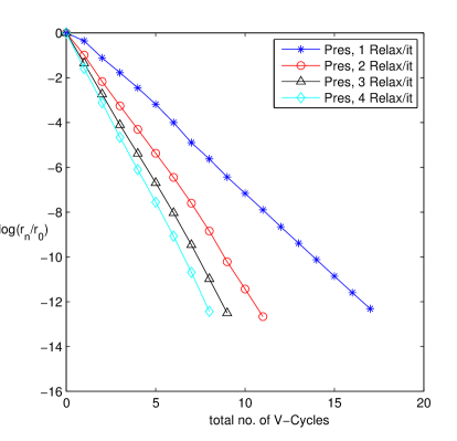
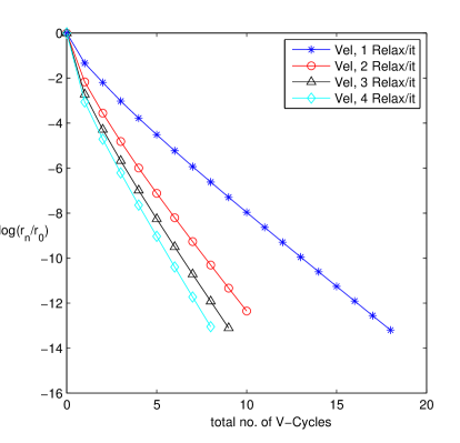
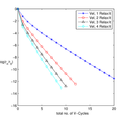
Fig. 1: The log of the relative residual for the pressure (left) and velocity (right) multigrid solvers as a function of the number of multigrid V cycles, for different numbers of smoothing (relaxation) sweeps. A constant coefficient steady Stokes problem is solved on a $512^{2}$ grid in two dimensions (top panels), and $128^{3}$ grid in three dimensions (bottom panels), with no-slip conditions at all domain boundaries.

In Fig. 1 we show the convergence of the pressure (left panels) and velocity multigrid solvers (right panels) for constant viscosity but for the stress-tensor form of the viscous term (21). In the upper row we show results in two dimensions, and in the lower row we show results for three dimensions. Similar results are obtained for different types of boundary conditions. We see a large increase in the rate of convergence when increasing the number of smoothing sweeps from one to two, and only a modest increase thereafter. Since the cost of geometric multigrid is in large part dominated by smoother, henceforth we use two applications of the smoother at each level of the multigrid hierarchy in each V cycle.

The speed of convergence of the multigrid iteration for the component solvers, is the standard against which one should measure convergence of the Krylov solver for the Stokes problem. As we can see in Fig. 1, each V cycle reduces the residual by at least an order of magnitude, so that only about a dozen V cycles are needed to reduce the residual to near roundoff. Therefore, a Stokes solver that uses only $10(d+1)$ scalar multigrid cycles to reduce the residual by more then 10 orders of magnitude should be considered excellent.

4.1.2 The effect of the number of multigrid cycles

As detailed in Appendix B, for constant-coefficient Stokes problems with periodic boundaries, GMRES will converge in a single iteration with preconditioner $\bm{P}_{1}$ and in two iterations with $\bm{P}_{2}$ and $\bm{P}_{3}$. The same holds for any choice of boundary condition for the time-dependent case in the inviscid limit. However, in the majority of cases of interest, multiple GMRES iterations will be required even if the subsolvers are exact. It is therefore important to explore the use of inexact pressure and velocity solvers. Specifically, it is important to determine the optimal number of multigrid V cycles per application of the preconditioner. We use the preconditioner $\bm{P}_{1}$ for these tests; similar results are observed for all of the preconditioners.

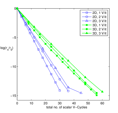
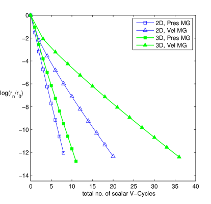
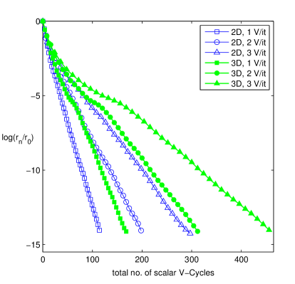
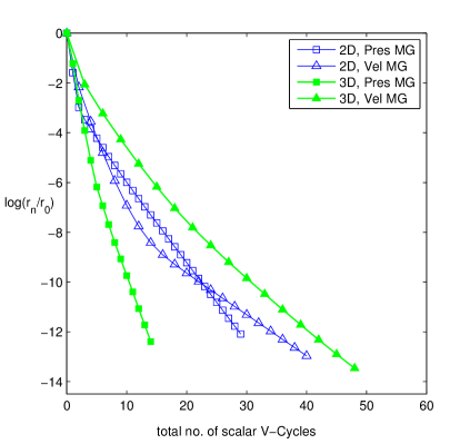
Fig. 2: The relative residual (on a log scale) as a function of the total number of scalar multigrid V cycles, for different number of multigrid cycles per application of the pressure and velocity subsolvers in preconditioner $\bm{P}_{1}$. GMRES convergence is shown in the left panels, and pressure (squares) and velocity (triangles) multigrid convergence is shown in the right panels, in both two ($512^{2}$ grid, empty symbols) and three ($128^{3}$ grid, filled symbols) dimensions. Restarts are not employed in the GMRES solver. The top panels show results for a constant-coefficient periodic steady-state Stokes problem, and the bottom panels show results for the bubble test problem.

In the left panels of Fig. 2 we show the convergence of the relative preconditioned residual, as estimated by the GMRES algorithm, for steady Stokes problems in two and three dimensions, as a function of the total number of scalar V cycles. We recall that the number of V cycles is a good proxy for the total computational effort, so that the most rapid convergence in these plots corresponds to the most efficient solvers. In the top left panel we show results for constant viscosity but for the stress-tensor form of the viscous term (21) for a periodic system, and in the bottom left panel we show results for the variable-viscosity bubble problem described earlier. In the corresponding right panels we show the convergence of the pressure and velocity multigrid subsolvers on the same problem, to serve as a reference point for what one may expect for a projection-like split solver.

The top left panel in Fig. 2 shows that for periodic constant coefficient problems there is no significant difference between using an exact subsolver (in effect, many V cycles per application of the preconditioner), and using only a single V cycle in the preconditioner but doing more GMRES iterations. This is not unexpected because the standard multigrid algorithm takes the form of a simple Richardson iterative solver, and we expect GMRES to perform at least as well as Richardson iteration. Note that for more difficult Poisson problems, such as problems with large jumps in the coefficients, it is well-known that a Krylov solver preconditioned with multigrid is more robust than multigrid alone, see for example the discussion in Ref. [21].

In the bottom left panel in Fig. 2 we show the convergence of GMRES for the variable-coefficient bubble problem, which is typical of the behavior we observe when there are non-periodic boundary conditions or variable coefficients. Similar behavior is observed for the other preconditioners (not shown). The results clearly demonstrate that when using exact subsolvers in the preconditioner does not yield an exact solver for the Stokes problem, the extra cost of performing more than a single V cycle of multigrid does not pay off in terms of overall efficiency. The optimal rate of convergence is observed when using only a single V cycle in the preconditioner. We have observed no advantage to using a different number of cycles in the pressure and velocity solvers, except for nearly inviscid problems where performing more than one pressure cycle may be somewhat beneficial. By comparing the left and right panels, we see that when using a single multigrid cycle in the preconditioner the total number of scalar V cycles is at most 2-3 times larger than that used in fractional step (projection) methods (for example, $\sim 50+15=65$ in three dimensions for projection methods as seen in the right panel, and $\sim 170$ cycles for coupled solver as seen in the left panel).

Based on these observations, henceforth we use only a single multigrid cycle in the subsolvers employed by the preconditioners.

4.2 Comparison of Preconditioners

Having empirically determined the optimal settings for the pressure and velocity subsolvers, we now turn to exploring the performance of the different preconditioners. We begin by settling an issue regarding the proper choice of sign in the upper/lower triangular and block-diagonal preconditioners.

4.2.1 The effect of the sign of Schur complement

In the literature [30, 35], the following Schur complement based preconditioners have been proposed and studied,

$$\bm{P}_{\pm}=\left(\begin{array}[]{cc}\bm{A}&\bm{0}\\ -\bm{D}&\pm(-\bm{D}\bm{A}^{-1}\bm{G})\end{array}\right),$$

where the sign of the lower diagonal block can be either positive or negative. It was proven that $\bm{T}_{+}=\bm{P}_{+}^{-1}\bm{M}$ satisfies $(\bm{T}_{+}-\bm{I})(\bm{T}_{+}+\bm{I})=\bm{0}$ and $\bm{T}_{-}=\bm{P}_{-}^{-1}\bm{M}$ satisfies $(\bm{T}_{-}-\bm{I})^{2}=\bm{0}$ [30, 35]. If a block-diagonal preconditioner such as $\bm{P}_{4}$ is used, by changing the sign it is possible to either make the preconditioned operator symmetric but indefinite (allowing the use of methods such as MINRES), or non-symmetric but positive semi-definite [20].

Because the GMRES method possesses a Galerkin property [15], the total number of GMRES iterations is equal to the degree of the characteristic polynomials of the preconditioned systems. Therefore, using both $\bm{P}_{+}^{-1}\bm{M}$ and $\bm{P}_{-}^{-1}\bm{M}$, GMRES converges in 2 iterations if the inverses of $\bm{A}$ and the Schur complement are exact [35]. However, when inexact subsolvers are employed, we observe significant difference between the two choices of the sign of the Schur complement. Our numerical results (not shown) indicate that the preconditioners with "-" sign in front of Schur complement give almost twice faster GMRES convergence than those with "+" sign. This is consistent with our original choice in Eqs. (17) and (19).

4.2.2 The effect of restarts

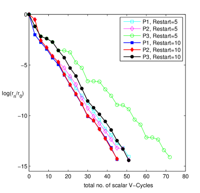
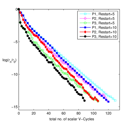
Fig. 3: The GMRES convergence history for preconditioners $\bm{P}_{1}$, $\bm{P}_{2}$ and $\bm{P}_{3}$ in two dimensions ($512^{2}$ grid) for the bubble test problem, for GMRES restart frequency 5 (open symbols) and 10 (filled symbols). In the left panel we set the viscosity to zero (unsteady inviscid flow) and in the right panel we set density to zero (steady viscous flow).

For large-scale problems, particularly in three dimensions, the memory requirements of the GMRES algorithm can be excessive. Restarts of the GMRES iteration offer a simple way not only to avoid convergence stalls, but also to limit the memory use. In Fig. 3 we compare the behavior of $\bm{P}_{1}$, $\bm{P}_{2}$ and $\bm{P}_{3}$ for restart intervals of 5 or 10 GMRES iterations. In the left panel of the figure we show the behavior for an inviscid time-dependent bubble test problem ($\bm{L}_{\bm{\mu}}=\bm{0}$, relevant to simulations of large Reynolds number flows) and in the right panel we show the behavior for a steady Stokes bubble problem (relevant to small Reynolds number flows). A two dimensional calculation is shown in the figure but similar results are observed in three dimensions as well. In the left panel of Fig. 3 we see that the performance of $\bm{P}_{3}$ significantly deteriorates for the small restart interval for the inviscid problem. In the right panel of the figure we see some deterioration of the convergence for the small restart interval for all three preconditioners.

Based on these results, henceforth we use a restart interval of 10 iterations.

4.2.3 Comparisons of different preconditioners

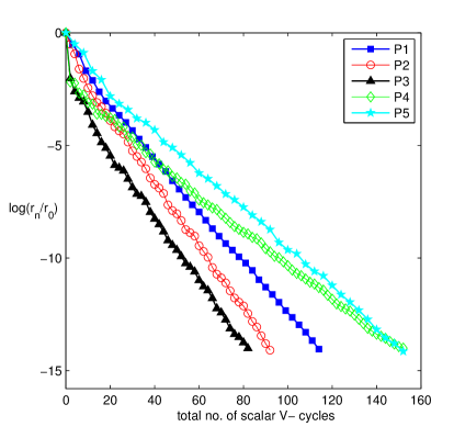
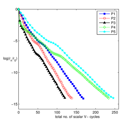
Fig. 4: The GMRES convergence history for preconditioners $\bm{P}_{1}$, $\bm{P}_{2}$, $\bm{P}_{3}$, $\bm{P}_{4}$ and $\bm{P}_{5}$ in two (left panel, $512^{2}$ grid) and three (right panel, $128^{3}$ grid) dimensions, for the bubble test problem. The restart frequency is 10 GMRES iterations.

Having empirically determined the optimal subsolver settings and the optimal sign of the Schur complement in the lower diagonal block of the preconditioners, we can now compare the performance of the five preconditioners on the bubble test problem in two and three dimensions. The GMRES convergence results shown in Fig. 4 demonstrate that for steady Stokes problem the lower and upper triangular preconditioners $\bm{P}_{2}$ and $\bm{P}_{3}$ yield the most efficient GMRES solver. The projection preconditioner $\bm{P}_{1}$ is seen to give robust convergence but is less efficient for the steady flow case because it requires one additional scalar (pressure) V cycle per GMRES iteration. The results in the figure also clearly show that $\bm{P}_{4}$ and $\bm{P}_{5}$ are much less efficient. This shows that including an upper or lower triangular block in the Schur complement based block preconditioners improves convergence, and also shows that the extra work in $\bm{P}_{5}$ over $\bm{P}_{1}$ is not justified in terms of overall efficiency, similarly to how the additional pressure solve in $\bm{P}_{1}$ does not yield improvement.

Based on these observations, henceforth we do not consider $\bm{P}_{4}$ and $\bm{P}_{5}$. Since we find very similar behavior between $\bm{P}_{2}$ and $\bm{P}_{3}$, while $\bm{P}_{3}$ shows poorer behavior with frequent restarts, henceforth we focus on examining in more detail the performance of $\bm{P}_{1}$ and $\bm{P}_{2}$.

4.3 Robustness

In this section we examine in more detail the robustness of $\bm{P}_{1}$ and $\bm{P}_{2}$ under varying importance of the viscous contribution to $\bm{A}$, and changing problem size.

4.3.1 Effects of viscous CFL number

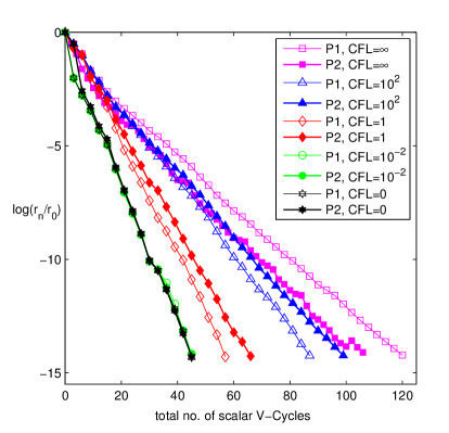
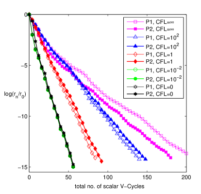
Fig. 5: The GMRES convergence history for preconditioners $\bm{P}_{1}$ (empty symbols) and $\bm{P}_{2}$ (filled symbols) in two dimensions (left panel, $512^{2}$ grid) and in three dimensions (right panel, $128^{3}$ grid) for the bubble test problem. We vary $\theta$ to change the viscous CFL number $\beta$ from the inviscid limit $\beta=0$ to the steady limit $\beta\rightarrow\infty$.

One of the goals of our study is to design preconditioners that work not just in the steady state limit but also for time-dependent problems. While one can use a suitably-defined Reynolds number to measure the importance of the inertial term $\theta{\bm{\rho}}$ in $\bm{A}$ relative to the viscous term $\bm{L}_{\bm{\mu}}$, the best dimensionless number to use for this is the viscous CFL number

$$\beta=\frac{\nu_{0}}{\theta h^{2}}=\frac{\mu_{0}}{\theta\rho_{0}h^{2}}.$$

A small $\beta\ll 1$ indicates an easier problem where inertial effects dominate, with $\beta=0$ corresponding to inviscid flow. A large $\beta>n_{c}^{2}$ indicates a viscous-dominated problem, where $n_{c}$ is the grid size, with the hardest case being a steady-state problem $\beta\rightarrow\infty$. In Fig. 5 we study the performance of the GMRES Stokes solver for varying viscous CFL numbers for the bubble test problem, in both two and three dimensions, for both preconditioners $\bm{P}_{1}$ and $\bm{P}_{2}$. As expected, we see most rapid convergence for $\beta=0$, and slowest convergence for $\beta\rightarrow\infty$. For the steady state case $\theta=0$, we do not need a pressure Poisson solve for $\bm{P}_{2}$ and therefore this preconditioner is somewhat more efficient than $\bm{P}_{1}$. For intermediate $\beta$’s we get somewhat better convergence for $\bm{P}_{1}$, although the difference is small. In our experience both preconditioners show rather robust behavior for varying viscous CFL number, viscosity and density contrast ratios, and different combinations of boundary conditions (periodic, free-slip, or no-slip).

4.3.2 Effects of problem size

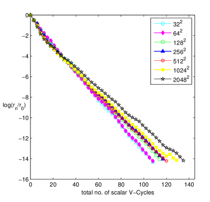
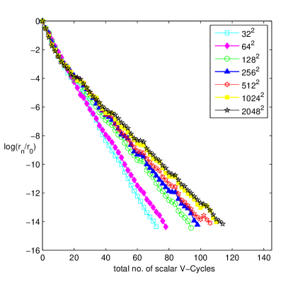
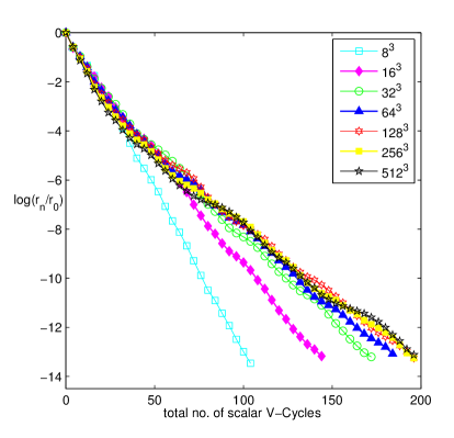
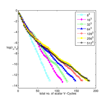
Fig. 6: The GMRES convergence history for preconditioners $\bm{P}_{1}$ (left panels) and $\bm{P}_{2}$ (right panels) in two dimensions (top panels) and in three dimensions (bottom panels) for the steady-state bubble test problem with contrast ratio $r_{\mu}=r_{\rho}=100$, as the grid size is varied.

An important goal in designing solvers suitable for large-scale calculations is to ensure that the total number of multigrid cycles remains essentially independent of the system size (or, equivalently, under grid refinement). In Fig. 6 we show convergence histories of GMRES for varying grid sizes for the steady state bubble problem in both two and three dimensions. In the left panels we show results for $\bm{P}_{1}$ and the right panels for $\bm{P}_{2}$. For this challenging variable-viscosity problem (recall that the viscosity and density contrast ratio is $r_{\mu}=r_{\rho}=100$), $\bm{P}_{1}$ shows robust convergence for all of the grid sizes tested here in both two and three dimensions, requiring no more than 200 multigrid V cycles (i.e., no more than $200/4=50$ GMRES iterations) to reduce the residual to essentially roundoff tolerance even for a $512^{3}$ grid. The convergence for preconditioner $\bm{P}_{2}$ shows a very mild deterioration with increasing system size, although the overall efficiency is still somewhat higher than $\bm{P}_{1}$ for all system sizes tested here. We have confirmed that making the subsolvers nearly exact does not aid the overall GMRES convergence, despite the substantial increase in the computational cost (data not shown).

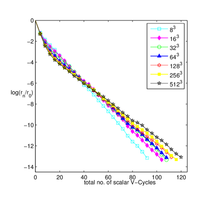
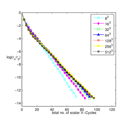
Fig. 7: Same as bottom two panels of Fig. 6 but for contrast ratio $r_{\mu}=r_{\rho}=2$.

It is important to point out that the exact convergence and its behavior on system size depends sensitively on the details of the multigrid algorithm (e.g., how the bottom level of the multigrid hierarchy is handled, which is typically affected by parallelization), the restart interval (here set to 10 iterations), and, most importantly, on the contrast ratio. In Fig. 7 we show scaling results in three dimensions for a much weaker contrast ratio $r_{\mu}=r_{\rho}=2$. In this case we see little to no effect of the system size on the convergence rate, and the total number of GMRES iterations is less than 30.

5 Conclusions

We studied several preconditioners for solving time-dependent and steady discrete Stokes problems arising when solving fluid flow problems on a staggered finite-volume grid. All of the preconditioners we studied are based on approximating the inverse of the Schur complement with a simple local operator and have been proposed before, though often limited to either constant coefficient or steady flow. By suitably approximating the inverse of the Schur complement in the case of time-dependent variable-viscosity flow we were able to easily generalize these preconditioners and thus substantially enlarge their practical applicability. Herein, we modified and extended a previously proposed projection-based preconditioner $\bm{P}_{1}$ to variable-coefficient flows [24], we generalized a well-known lower triangular preconditioner $\bm{P}_{2}$ to variable-coefficient flow, and we extended a previously-studied “fully coupled” solver with a “local viscosity” preconditioner [21] to time-dependent flows to obtain an upper triangular preconditioner $\bm{P}_{3}$. The preconditioners investigated here can be generalized to other stable or stabilized spatial discretizations of the time-dependent Stokes equations, such as finite-element schemes or adaptive mesh finite-volume discretizations.

Our primary focus was on studying the performance of these preconditioners when the pressure and velocity subsolvers are performed on a uniform staggered grid using geometric multigrid algorithms. We showed that optimal convergence rates of the GMRES Stokes solver were obtained when a single multigrid V cycle is employed as an inexact subdomain solver. We numerically observed that all three preconditioners are effective for both time-dependent and steady flow problems, with the lower and upper triangular preconditioners being more efficient for steady problems and $\bm{P}_{1}$ being somewhat more efficient for time-dependent problems, which is consistent with the findings of Ref. [24]. All three preconditioners were found to handle variable-coefficient problems rather well, with little deterioration in convergence from the case of constant-coefficient problems. Our observations are consistent with the conclusion of the authors of Ref. [21], who “find that it is advantageous to use the FC [fully-coupled] approach utilizing relaxed tolerances for solution of the sub-problems, combined with the LV [local viscosity] preconditioner.”

All of our empirical observations are consistent with the general observation that solving the coupled Stokes problem is comparable to a single step of a fractional step method, and not more than 2-3 times more expensive than a fractional step even for difficult cases of large contrast ratio, large viscous CFL number and non-trivial boundary conditions. We believe that this mild increase in cost is more than justified given the important advantages of the the coupled approach when solving the Navier-Stokes equations. Furthermore, we observed robust behavior of the projection and lower triangular preconditioners for large systems with relatively frequent restarts. This demonstrates that GMRES with preconditioners $\bm{P}_{1}$ and $\bm{P}_{2}$ provides a robust solver for large-scale computations. In future studies, the robustness of these preconditioners with respect to the variability of viscosity and density should be studied more carefully. One aspect of this is whether the spectrum of the preconditioned operator can be provably bounded for arbitrary contrast ratios. More importantly, however, the performance of the preconditioners in practical applications, should be accessed. Experience with steady Stokes geodynamics applications, which have extreme viscosity contrasts, are very promising [21].

Acknowledgments

We thank Howard Elman for informative discussions. A. Donev and M. Cai were supported in part by the NSF under grant DMS-1115341. Additional support for A. Donev was provided by the DOE Office of Science through Early Career award DE-SC0008271. B. E. Griffith acknowledges research support from the National Science Foundation under awards OCI 1047734 and DMS 1016554. J. Bell and A. Nonaka were supported by the DOE Applied Mathematics Program of the DOE Office of Advanced Scientific Computing Research under the U.S. Department of Energy under contract No. DE-AC02-05CH11231.

Appendix A Fourier Analysis of Schur Complement

The most important element in the preconditioners we study here is the approximation of the Schur complement inverse. In previous work, Fourier analysis [9], operator mapping properties and PDE theory in [33, 34], and commutator properties (8) [31, 16, 24] have been used to justify approximations to the Schur complement inverse. Here we use Fourier analysis to justify our approximation to the Schur complement inverse for the stress form of the viscous operator (21). This analysis assumes periodic boundaries but should also inform the case with physical boundary conditions.

For simplicity, we use two dimensional steady state Stokes equations for illustration but extensions to three dimensions and time-dependent flow are trivial. We denote the discrete Fourier transform of velocity as $\hat{\bm{v}}=\left[\hat{u},\,\hat{v}\right]^{T}$, and denote the (purely imaginary) Fourier symbol of the staggered divergence operator as $\hat{\bm{D}}=[\hat{\bm{D}}_{x}~{}\hat{\bm{D}}_{y}]$, where $\bm{D}_{x}$ and $\bm{D}_{y}$ represent the staggered finite difference operator along the $x$ and $y$ axes. The Fourier transform of the staggered gradient operator is $\hat{\bm{G}}=-\hat{\bm{D}}^{\star}=[\hat{\bm{D}}_{x}~{}\hat{\bm{D}}_{y}]^{T}$, and similarly,

$$\hat{L}_{p}=\hat{\bm{D}}\hat{\bm{G}}=\hat{\bm{D}}_{x}^{2}+\hat{\bm{D}}_{y}^{2}=-\left(\left|\hat{\bm{D}}_{x}\right|^{2}+\left|\hat{\bm{D}}_{y}\right|^{2}\right).$$

Our goal is to approximate the Schur complement inverse with a Laplacian-like local operator $\bm{L}_{\bm{S}}$, i.e., to find $(\bm{D}\bm{L}_{{\bm{\mu}}}^{-1}\bm{G})^{-1}=\bm{L}_{\bm{S}}.$ This is only an approximation in general but should be exact for periodic constant-coefficient problems. In Fourier space,

$${\displaystyle\hat{\bm{L}}_{\bm{S}}=\left(\hat{\bm{D}}\hat{\bm{L}}_{\bm{\mu}}^{-1}\hat{\bm{G}}\right)^{-1}.}$$ (24)

When the Laplacian form of the viscous term is used, $\bm{L}_{{\bm{\mu}}}=\mu_{0}\bm{L}$, we have

$${\displaystyle\hat{\bm{L}}_{\bm{\mu}}=\mu_{0}\left[\begin{array}[]{cc}\hat{\bm{D}}_{x}^{2}+\hat{\bm{D}}_{y}^{2}&0\\ 0&\hat{\bm{D}}_{x}^{2}+\hat{\bm{D}}_{y}^{2}\end{array}\right]},$$

which combined with (24) gives $\hat{\bm{L}}_{\bm{S}}=\mu_{0}.$ Applying an inverse Fourier transform gives the well-known result $\bm{L}_{\bm{S}}=\mu_{0}\bm{I}.$

When $\bm{L}_{{\bm{\mu}}}$ is the discrete operator for the stress tensor form of the viscous term (21) and the viscosity is constant, we have

$${\displaystyle\hat{\bm{L}}_{\bm{\mu}}=\mu_{0}\left[\begin{array}[]{cc}2\hat{\bm{D}}_{x}^{2}+\hat{\bm{D}}_{y}^{2}&\hat{\bm{D}}_{y}\hat{\bm{D}}_{x}\\ \hat{\bm{D}}_{x}\hat{\bm{D}}_{y}&\hat{\bm{D}}_{x}^{2}+2\hat{\bm{D}}_{y}^{2}\end{array}\right]},$$

which gives $\hat{\bm{L}}_{\bm{S}}=2\mu_{0},$ and therefore $\bm{L}_{\bm{S}}=2\mu_{0}\bm{I}$. This motivates our variable-viscosity generalization (10). When $\bm{L}_{{\bm{\mu}}}$ is the discrete operator for the viscous term with bulk viscosity and assuming both the shear viscosity and the bulk viscosities are constant, we have

$${\displaystyle\hat{\bm{L}}_{\bm{\mu}}=\left[\begin{array}[]{cc}(\frac{4}{3}\mu_{0}+\gamma_{0})\hat{\bm{D}}_{x}^{2}+\mu_{0}\hat{\bm{D}}_{y}^{2}&(\frac{1}{3}\mu_{0}+\gamma_{0})\hat{\bm{D}}_{y}\hat{\bm{D}}_{x}\\ (\frac{1}{3}\mu_{0}+\gamma_{0})\hat{\bm{D}}_{x}\hat{\bm{D}}_{y}&\gamma_{0}\hat{\bm{D}}_{x}^{2}+(\frac{4}{3}\mu_{0}+\gamma_{0})\hat{\bm{D}}_{y}^{2}\end{array}\right],}$$

which gives $\hat{\bm{L}}_{\bm{S}}=\left(\frac{4}{3}\mu_{0}+\gamma_{0}\right)$ and therefore ${\displaystyle\bm{L}_{\bm{S}}=\left(\frac{4}{3}\mu_{0}+\gamma_{0}\right)\bm{I}}$. This motivates our variable-viscosity generalization (11).

Appendix B Analysis of preconditioners with exact subsolvers

In this Appendix we give some analysis of the spectrum of the preconditioned operators when exact pressure and velocity subsolvers are used. To see how well the different preconditioners approximate the original saddle point form (5), we formally calculate

$$\bm{P}_{1}^{-1}\bm{M} = \left(\begin{array}[]{cc}\bm{I}&(\bm{I}-\bm{\rho}^{-1}\bm{G}\bm{L}_{\bm{\rho}}^{-1}\bm{D})\bm{A}^{-1}\bm{G}\\ \bm{0}&\mathcal{S}^{-1}\bm{S}\end{array}\right),$$ (27)

$$\bm{P}_{2}^{-1}\bm{M} = \left(\begin{array}[]{cc}\bm{I}&\bm{A}^{-1}\bm{G}\\ \bm{0}&\mathcal{S}^{-1}\bm{S}\end{array}\right),$$ (30)

$$\bm{P}_{3}^{-1}\bm{M} = \left(\begin{array}[]{cc}\bm{I}-\bm{A}^{-1}\bm{G}\mathcal{S}^{-1}\bm{D}&\bm{A}^{-1}\bm{G}\\ \mathcal{S}^{-1}\bm{D}&\bm{0}\end{array}\right),$$ (33)

and lastly

$$\bm{P}_{4}^{-1}\bm{M} = \left(\begin{array}[]{cc}\bm{I}&\bm{A}^{-1}\bm{G}\\ \mathcal{S}^{-1}\bm{D}&\bm{0}\end{array}\right).$$ (36)

Recall that for constant-coefficient problems with exact subsolvers, $\mathcal{S}^{-1}=-\theta\rho_{0}\bm{L}_{p}^{-1}+\mu_{0}\bm{I}$. For periodic domains, the finite-difference operators $\bm{G}$, $\bm{D}$, $\bm{L}$ and $\bm{L}_{p}$ commute,

$$\bm{G}\bm{L}_{p}=\bm{L}\bm{G}\quad\mbox{and}\quad\bm{L}_{p}\bm{D}=\bm{D}\bm{L},$$ (37)

and therefore $\bm{P}_{1}^{-1}\bm{M}$ is exactly the discrete identity operator, and similarly, the (1,1) diagonal block of $\bm{P}_{3}^{-1}\bm{M}$ is zero.

From (27), we see that the preconditioned system is block upper triangular. Therefore, the eigenvalues of the preconditioned system are either unity or the eigenvalues of $\mathcal{S}^{-1}\bm{S}$. Similarly, we can derive the eigenvalues of the preconditioned system using (30) and (33). Alternatively, one can write down the generalized eigenvalue system, for instance,

$$\bm{M}\left(\begin{array}[]{c}\bm{u}\\ p\end{array}\right)=\lambda\bm{P}_{3}\left(\begin{array}[]{c}\bm{u}\\ p\end{array}\right)$$

Again, one can see that the eigenvalues are either 1 or the eigenvalues of $\mathcal{S}^{-1}\bm{S}$.

When $\mu_{0}=0$, or equivalently, $\Delta t\rightarrow 0$, we have that $\bm{P}_{1}^{-1}\bm{M}=\bm{I}$, regardless of the boundary conditions. If $\bm{P}_{2}$ is used, we have

$$\bm{P}_{2}^{-1}\bm{M} = \left(\begin{array}[]{cc}\bm{I}&\frac{\Delta t}{\rho_{0}}\bm{G}\\ \bm{0}&\bm{I}\end{array}\right),$$ (40)

and therefore $(\bm{P}_{2}^{-1}\bm{M}-\bm{I})^{2}=\bm{0}$. This proves that in the inviscid case, the GMRES algorithm converges in 1 iteration when preconditioner $\bm{P}_{1}$ is used, and in 2 iterations when $\bm{P}_{2}$ or $\bm{P}_{3}$ are used. When inexact subsolvers are used our numerical results showed that all three preconditioners exhibit exactly the same convergence rate in the inviscid case.

Furthermore, for constant viscosity ($\mu=1$) steady state ($\theta=0$) problems on a two-dimensional domain of $n_{x}\times n_{y}$ grid cells with no-slip boundaries, one can prove the following property for the eigenvalues of the Schur complement $\bm{S}=\bm{D}\bm{L}^{-1}\bm{G}$:

1. $\lambda(\bm{S})\in\{0\}\cup[\eta^{2},1]$, where $\eta$ is the inf-sup constant independent of grid size [19, 37].

2. The multiplicity of the 0 eigenvalue is 1.

3. There are at most $2(n_{x}-1)+2(n_{y}-1)$ non-unit eigenvalues of $\bm{S}$.

This is a quantitative statement of the intuitive expectation that a few cells away from the boundaries $\bm{S}$ is close to an identity operator, just as for a periodic system (see Eq. (37)). The lower bound of the eigenvalues is a consequence of the uniform div-stability [18, 19, 47]. From (27) (and also (30) and (33)), we see that the same conclusions hold for the preconditioned systems. This analysis explains the good performance of the simple Schur complement approximation even in the presence of nontrivial boundary conditions [24]. Below we numerically compute the spectrum of the eigenvalues of $\mathcal{S}^{-1}\bm{S}$ for both constant and variable viscosity steady flow, and confirm the theoretical predictions above.

B.1 Spectrum of the Preconditioned Operator

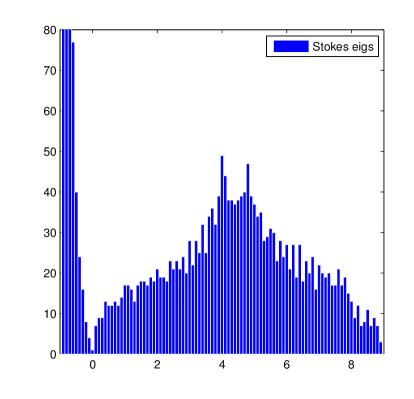
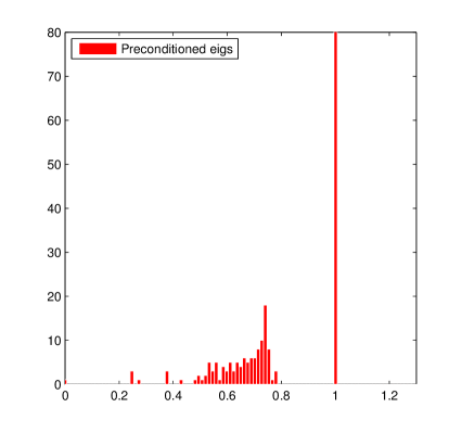
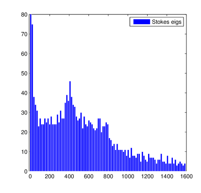
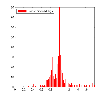
Fig. 8: Histogram of the eigenvalues of $\bm{M}$ (left panels) and $\bm{P}^{-1}\bm{M}$ (more precisely, $\mathcal{S}^{-1}\bm{S}$) (right panels) for a steady Stokes problem on a grid of $32\times 32$ cells with four no-slip boundaries. The vertical axis gives the number of eigenvalues, truncated for the eigenvalue $\lambda=1$ in the right panels due to the large number of unit eigenvalues. The case of constant viscosity is shown in the upper panels, and the case of variable viscosity with contrast ratio $100$ is shown in the lower panels.

Convergence analysis of the preconditioned GMRES method is not straightforward and there is no simple link to the spectrum of the eigenvalues. Nevertheless, it is generally accepted and widely observed that having closely clustered eigenvalues of the preconditioned operator $\bm{P}^{-1}\bm{M}$ leads to faster convergence. Furthermore, the ratio of the largest to the smallest eigenvalue (excluding the trivial zero eigenvalue arising from the fact pressure is only determined up to a constant) should be bounded from above by a constant essentially independent of grid size, and, possibly, viscosity and density contrast ratio.

We focus on the steady-flow case $\theta=0$ in two dimensions, for a square domain of $n_{c}^{2}$ cells with four no-slip boundaries. We consider using exact subdomain solvers, $\widetilde{\bm{A}}^{-1}=\bm{A}^{-1}$ and $\widetilde{\bm{L}}_{\bm{\rho}}^{-1}=\bm{L}_{\rho}^{-1}$ instead of multigrid, relying on the fact that a well-designed multigrid cycle is (essentially) spectrally-equivalent to an exact solver. We explicitly form $\bm{M}$ and $\mathcal{S}^{-1}\bm{S}$ in MATLAB as dense matrices and compute their eigenvalues.

In Fig. 8, we show a histogram of the eigenvalues of the unpreconditioned and preconditioned operators for a square domain of length $n_{c}=32$ cells with no-slip boundaries. In the upper row in Fig. 8 we study the constant viscosity case. The total number of DOFs is $N_{\text{dof}}=n_{c}^{2}+2n_{c}\left(n_{c}-1\right)=3008$. Since the original Stokes system is of saddle point type, $\bm{M}$ has both positive eigenvalues and negative eigenvalues, and there are $n_{c}^{2}=1024$ eigenvalues that are smaller than or equal to zero. While the unpreconditioned spectrum shows a broad spectrum of eigenvalues with conditioning number that grows with the grid size, the preconditioned spectrum shows that most eigenvalues are unity, with the remaining $4\left(n_{c}-1\right)/N_{\text{dof}}\approx 4\%$ nonzero eigenvalues remaining well-clustered.

In the lower row in Fig. 8 we study the variable viscosity case for the bubble problem with viscosity contrast ratio $r_{\mu}=100$. The unpreconditioned system is seen to be very badly conditioned, with a broad spectrum of eigenvalues. By contrast, the preconditioned operator is well-conditioned, with around 87% of the eigenvalues in the interval $\left(0.99,1.01\right)$. While some eigenvalues are larger than unity in this case, the spread in the eigenvalues is not much different from the constant-coefficient case. This suggests that the spectrum remains localized around unity and bounded away from zero even for rather large contrast ratios. It may be possible to extend the finite-element theory developed in Refs. [27, 26] to prove that $\mathcal{S}^{-1}\bm{S}$ is spectrally-equivalent to the identity matrix for the staggered grid discretization we employ here.

Appendix C Multigrid algorithms

We employ a standard V-cycle multigrid approach [6] for both the cell-centered multigrid subsolver for the weighted Poisson operator $\bm{L}_{\bm{\rho}}$ and the staggered velocity multigrid subsolver for the viscous operator $\bm{L}_{\bm{\mu}}$. We use the standard residual formulation, so that on all coarsened levels we are solving for the error in the coarsened residual from the next-finer level. In our implementation, the multigrid coarsening factor is 2, and coarsening continues until the problem domain represented on the coarsest grid contains two grid points (with respect to cell-centers) in any given spatial direction. At the coarsest level of the multigrid hierarchy, we perform a large (8 or more) number of relaxations, to ensure that the preconditioner is a constant linear operator.

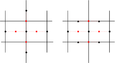
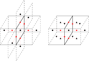
Fig. 9: (Left panel) The stencils for the $x$-component of $\bm{\nabla}\cdot\beta\bm{\nabla}\bm{\phi}$ (left) and $\bm{\nabla}\cdot\beta(\bm{\nabla}\bm{\phi})^{T}$ (right), in two dimensions. The black circles indicate locations of $u$. The black triangles indicate locations of $v$. The red dots indicate the location of the $\beta$ and the gradients of velocity. (Right panel) The stencils for the $x$-component of $\bm{\nabla}\cdot\beta\bm{\nabla}\bm{v}$ (left) and $\bm{\nabla}\cdot\beta(\bm{\nabla}\bm{v})^{T}$ (right), in three dimensions. The black circles indicate locations of $u$. The black triangles indicate locations of $v$ and $w$. The red dots indicate the location of the $\beta$ and the gradients of velocity.

Multigrid consists of 3 major components: (i) choice of relaxation at a particular level, (ii) coarsening/restriction operator, and (iii) interpolation/prolongation operator.

Relaxation. Both the staggered and cell-centered solvers use multicolored Gauss-Seidel smoothing. The cell-centered solver uses standard red-black relaxation, whereas the staggered solver uses a $2d$-colored relaxation, where $d$ is the dimensionality of the problem. Because the coupling between the degrees of freedom corresponding to a given component of velocity is the same as for the cell-centered Poisson equation, by coloring each component of the velocity separately, as in the standard red-black coloring (i.e., coloring odd grid points with a different color from the even grid points), we obtain decoupling between the $2d$ colors so that each color can be relaxed separately (improving convergence and aiding parallelization). We relax the components of velocity in turn (i.e., in three dimensions, we order the relaxations as red-$x$, black-$x$, red-$y$, black-$y$, red-$z$, black-$z$), although other orderings of the colors are possible. Refer to Figure 9 for a physical representation of the viscous operator stencils. Given a cell-centered operator of the form, $\bm{\nabla}\cdot\beta\bm{\nabla}\phi\equiv\mathcal{L}\phi=r$, or a staggered operator of the form, $\alpha\phi-\bm{\nabla}\cdot\beta[\bm{\nabla}\phi+(\bm{\nabla}\phi)^{T}]\equiv\mathcal{L}\phi=r$, the relaxation takes the form

$$\phi^{k+1}=\phi^{k}+\omega\mathcal{D}^{-1}(r-\mathcal{L}\phi^{k}),$$ (41)

for each color in turn, where the superscript represents the iterate, and $\mathcal{D}^{-1}$ is the inverse of the diagonal elements of $\mathcal{L}$. We use unit weighting factor, $\omega=1$ (suggested to be near-optimal in numerical experiments) for both subsolvers.

Restriction. For the cell-centered solver, restriction is a simple averaging of the $2^{d}$ fine cells. For the staggered solver, we use a slightly more complicated 6-point ($d=2$) or 12-point ($d=3$) stencil. For example, for $x$-faces we use

$$\phi_{i,j}^{{\rm c}}=\frac{1}{8}\left(\phi_{2i-1,2j}^{{\rm f}}+\phi_{2i-1,2j+1}^{{\rm f}}+\phi_{2i+1,2j}^{{\rm f}}+\phi_{2i+1,2j+1}^{{\rm f}}\right)+\frac{1}{4}\left(\phi_{2i,2j}^{{\rm f}}+\phi_{2i,2j+1}^{{\rm f}}\right)$$ (42)

As seen in Figure 9, for the staggered solver we require $\alpha$ at faces, and $\beta$ at both cell-centers and nodes ($d=2$) or edges ($d=3$). When creating coefficients at coarser levels, we obtain $\alpha$ by averaging the overlaying fine faces, cell-centered $\beta$ by averaging the overlaying fine cell-centered values, $\beta$ on nodes through direct injection, and $\beta$ on edges by averaging the overlaying fine edges.

Prolongation. For the cell-centered solver, prolongation is simply direct injection from the coarse cell to the overlaying $2^{d}$ fine cells. For the staggered solver, we use a slightly more complicated stencil that involves linear interpolation for fine faces that overlay coarse faces, and bilinear interpolation for fine faces that do not overlay coarse faces. For example, for $x$-faces we use

$$\phi_{i,j}^{{\rm f}}=\frac{3}{4}\phi_{i/2,j/2}^{{\rm c}}+\frac{1}{4}\phi_{i/2,j/2-1}^{{\rm c}},\quad\mbox{for }i\mbox{ and }j\mbox{ both even},$$ (43)

$$\phi_{i,j}^{{\rm f}}=\frac{3}{8}\left(\phi_{i/2,j/2}^{{\rm c}}+\phi_{i/2+1,j/2}^{{\rm c}}\right)+\frac{1}{8}\left(\phi_{i/2,j/2-1}^{{\rm c}}+\phi_{i/2+1,j/2-1}^{{\rm c}}\right),\quad\mbox{for }i\mbox{ odd and }j\mbox{ even},$$ (44)

where we use integer division in the index subscripts.

References

- [1] A. S. Almgren, J. B. Bell, P. Colella, L. H. Howell, and M. L. Welcome, A conservative adaptive projection method for the variable density incompressible Navier-Stokes equations, J. Comput. Phys., 142 (1998), pp. 1–46.
- [2] A. S. Almgren, J. B. Bell, and W. G. Szymczak, A numerical method for the incompressible Navier-Stokes equations based on an approximate projection, SIAM J. Sci. Comput., 17 (1996), pp. 358–369.
- [3] J. B. Bell, P. Colella, and H. M. Glaz, A second order projection method for the incompressible Navier-Stokes equations, J. Comp. Phys., 85 (1989), pp. 257–283.
- [4] M. Benzi, Preconditioning techniques for large linear systems: a survey, Journal of Computational Physics, 182 (2002), pp. 418–477.
- [5] M. Benzi, G. H. Golub, and J. Liesen, Numerical solution of saddle point problems, Acta numerica, 14 (2005), pp. 1–137.
- [6] W. L. Briggs, V. Henson, and S. McCormick, A multigrid tutorial society for industrial and applied mathematics, Philadelphia, PA, (1987).
- [7] D. L. Brown, R. Cortez, and M. L. Minion, Accurate projection methods for the incompressible Navier-Stokes equations, Journal of Computational Physics, 168 (2001), pp. 464–499.
- [8] C. Burstedde, O. Ghattas, G. Stadler, T. Tu, and L. C. Wilcox, Parallel scalable adjoint-based adaptive solution of variable-viscosity stokes flow problems, Computer Methods in Applied Mechanics and Engineering, 198 (2009), pp. 1691–1700.
- [9] J. Cahouet and J.-P. Chabard, Some fast 3d finite element solvers for the generalized stokes problem, International Journal for Numerical Methods in Fluids, 8 (1988), pp. 869–895.
- [10] A. J. Chorin, Numerical Solution of the Navier-Stokes Equations, J. Math. Comp., 22 (1968), pp. 745–762.
- [11] S. Delong, B. E. Griffith, E. Vanden-Eijnden, and A. Donev, Temporal Integrators for Fluctuating Hydrodynamics, Phys. Rev. E, 87 (2013), p. 033302.
- [12] A. Donev, T. G. Fai, and E. Vanden-Eijnden, The importance of hydrodynamic fluctuations for diffusion in liquids. Submitted to JSTAT, ArXiv preprint 1312.1894, 2013.
- [13] A. Donev, A. J. Nonaka, Y. Sun, T. G. Fai, A. L. Garcia, and J. B. Bell, Low Mach Number Fluctuating Hydrodynamics of Diffusively Mixing Fluids. Submitted to CAMCOS, ArXiv preprint 1212.2644, 2013.
- [14] W. E and J. Liu, Gauge method for viscous incompressible flows, Commun. Math. Sci., 1 (2003), pp. 317–332.
- [15] M. Eiermann and O. G. Ernst, Geometric aspects of the theory of krylov subspace methods, Acta Numerica, 10 (2001), pp. 251–312.
- [16] H. Elman, V. E. Howle, J. Shadid, R. Shuttleworth, and R. Tuminaro, Block preconditioners based on approximate commutators, SIAM Journal on Scientific Computing, 27 (2006), pp. 1651–1668.
- [17] , A taxonomy and comparison of parallel block multi-level preconditioners for the incompressible navier–stokes equations, Journal of Computational Physics, 227 (2008), pp. 1790–1808.
- [18] H. C. Elman, Preconditioning for the steady-state navier–stokes equations with low viscosity, SIAM Journal on Scientific Computing, 20 (1999), pp. 1299–1316.
- [19] H. C. Elman, D. J. Silvester, and A. J. Wathen, Finite Elements and Fast Iterative Solvers: with Applications in Incompressible Fluid Dynamics: with Applications in Incompressible Fluid Dynamics, OUP Oxford, 2005.
- [20] B. Fischer, A. Ramage, D. J. Silvester, and A. J. Wathen, Minimum residual methods for augmented systems, BIT Numerical Mathematics, 38 (1998), pp. 527–543.
- [21] M. Furuichi, D. A. May, and P. J. Tackley, Development of a stokes flow solver robust to large viscosity jumps using a schur complement approach with mixed precision arithmetic, Journal of Computational Physics, 230 (2011), pp. 8835–8851.
- [22] T. Geenen, C. Vuik, G. Segal, S. MacLachlan, et al., On iterative methods for the incompressible stokes problem, International Journal for Numerical methods in fluids, 65 (2011), pp. 1180–1200.
- [23] T. V. Gerya, D. A. May, and T. Duretz, An adaptive staggered grid finite difference method for modeling geodynamic Stokes flows with strongly variable viscosity, Geochemistry, Geophysics, Geosystems, 14 (2013), pp. 1200–1225.
- [24] B. Griffith, An accurate and efficient method for the incompressible Navier-Stokes equations using the projection method as a preconditioner, J. Comp. Phys., 228 (2009), pp. 7565–7595.
- [25] , Immersed boundary model of aortic heart valve dynamics with physiological driving and loading conditions, Int J Numer Meth Biomed Eng, 28 (2012), pp. 317–345.
- [26] P. Grinevich, An iterative solution method for the stokes problem with variable viscosity, Moscow University Mathematics Bulletin, 65 (2010), pp. 119–122.
- [27] P. Grinevich and M. Olshanskii, An iterative method for the stokes-type problem with variable viscosity, SIAM Journal on Scientific Computing, 31 (2009), pp. 3959–3978.
- [28] J. Guermond, P. Minev, and J. Shen, An overview of projection methods for incompressible flows, Computer Methods in Applied Mechanics and Engineering, 195 (2006), pp. 6011–6045.
- [29] F. Harlow and J. Welch, Numerical calculation of time-dependent viscous incompressible flow of fluids with free surfaces, Physics of Fluids, 8 (1965), pp. 2182–2189.
- [30] I. C. Ipsen, A note on preconditioning nonsymmetric matrices, SIAM Journal on Scientific Computing, 23 (2001), pp. 1050–1051.
- [31] D. Kay, D. Loghin, and A. Wathen, A preconditioner for the steady-state navier–stokes equations, SIAM Journal on Scientific Computing, 24 (2002), pp. 237–256.
- [32] D. A. Kay, P. M. Gresho, D. F. Griffiths, and D. J. Silvester, Adaptive time-stepping for incompressible flow part ii: Navier-stokes equations, SIAM Journal on Scientific Computing, 32 (2010), pp. 111–128.
- [33] K.-A. Mardal and R. Winther, Uniform preconditioners for the time dependent stokes problem, Numerische Mathematik, 98 (2004), pp. 305–327.
- [34] , Preconditioning discretizations of systems of partial differential equations, Numerical Linear Algebra with Applications, 18 (2011), pp. 1–40.
- [35] M. F. Murphy, G. H. Golub, and A. J. Wathen, A note on preconditioning for indefinite linear systems, SIAM Journal on Scientific Computing, 21 (2000), pp. 1969–1972.
- [36] M. Olshanskii, Multigrid analysis for the time dependent stokes problem, Mathematics of Computation, 81 (2012), pp. 57–79.
- [37] M. A. Olshanskii and E. V. Chizhonkov, On the best constant in the inf-sup-condition for elongated rectangular domains, Mathematical Notes, 67 (2000), pp. 325–332.
- [38] M. A. Olshanskii, J. Peters, and A. Reusken, Uniform preconditioners for a parameter dependent saddle point problem with application to generalized stokes interface equations, Numerische Mathematik, 105 (2006), pp. 159–191.
- [39] R. Pember, L. Howell, J. Bell, P. Colella, W. Crutchfield, W. Fiveland, and J. Jessee, An adaptive projection method for unsteady, low-Mach number combustion, Combustion Science and Technology, 140 (1998), pp. 123–168.
- [40] A. Quarteroni, F. Saleri, and A. Veneziani, Factorization methods for the numerical approximation of navier–stokes equations, Computer methods in applied mechanics and engineering, 188 (2000), pp. 505–526.
- [41] C. Rendleman, V. Beckner, M. Lijewski, W. Crutchfield, and J. Bell, Parallelization of structured, hierarchical adaptive mesh refinement algorithms, Computing and Visualization in Science, 3 (2000), pp. 147–157. Software available at https://ccse.lbl.gov/BoxLib.
- [42] Y. Saad, A flexible inner-outer preconditioned gmres algorithm, SIAM Journal on Scientific Computing, 14 (1993), pp. 461–469.
- [43] Y. Saad and M. H. Schultz, Gmres: A generalized minimal residual algorithm for solving nonsymmetric linear systems, SIAM Journal on scientific and statistical computing, 7 (1986), pp. 856–869.
- [44] D. Shin and J. C. Strikwerda, Inf-sup conditions for finite-difference approximations of the Stokes equations, Journal of the Australian Mathematical Society-Series B, 39 (1997), pp. 121–134.
- [45] S. Turek, Efficient Solvers for Incompressible Flow Problems: An Algorithmic and Computional Approach, vol. 6, Springer Verlag, 1999.
- [46] F. B. Usabiaga, J. B. Bell, R. Delgado-Buscalioni, A. Donev, T. G. Fai, B. E. Griffith, and C. S. Peskin, Staggered Schemes for Fluctuating Hydrodynamics, SIAM J. Multiscale Modeling and Simulation, 10 (2012), pp. 1369–1408.
- [47] R. Verfürth, A multilevel algorithm for mixed problems, SIAM journal on numerical analysis, 21 (1984), pp. 264–271.