Plasma effects on fast pair beams II. Reactive versus kinetic instability of parallel electrostatic waves

Abstract

The interaction of TeV gamma rays from distant blazars with the extragalactic background light produces relativistic electron-positron pair beams by the photon-photon annihilation process. Using the linear instability analysis in the kinetic limit, which properly accounts for the longitudinal and the small but finite perpendicular momentum spread in the pair momentum distribution function, the growth rate of parallel propagating electrostatic oscillations in the intergalactic medium is calculated. Contrary to the claims of Miniati and Elyiv (2013) we find that neither the longitudinal nor the perpendicular spread in the relativistic pair distribution function do significantly affect the electrostatic growth rates. The maximum kinetic growth rate for no perpendicular spread is even about an order of magnitude greater than the corresponding reactive maximum growth rate. The reduction factors to the maximum growth rate due to the finite perpendicular spread in the pair distribution function are tiny, and always less than $10^{-4}$. We confirm the earlier conclusions by Broderick et al. (2012) and us, that the created pair beam distribution function is quickly unstable in the unmagnetized intergalactic medium. Therefore, there is no need to require the existence of small intergalactic magnetic fields to scatter the produced pairs, so that the explanation (made by several authors) of the FERMI non-detection of the inverse Compton scattered GeV gamma rays by a finite deflecting intergalactic magnetic field is not necessary. In particular, the various derived lower bounds for the intergalactic magnetic fields are invalid due to the pair beam instability argument.

1. Introduction

The new generation of air Cherenkov TeV $\gamma$-ray telescopes (HESS, MAGIC, VERITAS) have detected about 30 cosmological blazars with strong TeV photon emission: the most distant ones are 3C279 (redshift $z_{r}=0.536$), 3C66A ($z_{r}=0.444$) and PKS 1510-089 ($z_{r}=0.361$). Any of these more distant than $z_{r}=0.16$ produces energetic $e^{\pm}$ particle beams in double photon collisions with the extragalactic background light (EBL). These pairs with typical Lorentz factors $\gamma=10^{6}\Gamma_{6}$ are expected to inverse Compton (IC) scatter on the cosmic microwave background (CMB) radiation, on a typical length scale $l_{IC}\sim 0.75\Gamma_{6}^{-1}$ Mpc, thus producing gamma-rays with energy of order 100 GeV, which have not been detected by the FERMI satellite. Given the still relatively short distance $l_{IC}$, both pair production and IC emission occur primarily in cosmic voids of the intergalactic medium (IGM), which fill most of cosmic volume. It has been argued that the inverse Compton scattered gamma-rays then are still energetic enough for further pair-production interactions giving rise to a full electromagnetic cascade as in vacuum.

However, the pair-beam is subject to two-stream-like instabilities of both electrostatic and electromagnetic nature (Broderick et al. 2012, Schlickeiser et al. 2012a). In this case the electromagnetic pair cascade does not contribute to the multi-GeV flux, as most of the pair beam energy is transferred to the IGM with important consequences for its thermal history. Moreover, there is no need to require the existence of small intergalactic magnetic fields to scatter the produced pairs, so that the explanation of the FERMI non-detection of the inverse Compton scattered GeV gamma rays by a finite deflecting intergalactic magnetic field (Neronov and Vovk 2010, Tavecchio et al. 2011, Dolag et al. 2011, Taylor et al. 2012, Dermer et al. 2011, Takahashi et al. 2012, Vovk et al. 2012) is not necessary.

In their instability analysis Schlickeiser et al. (2012a – hereafter referred to as paper I) and Broderick et al. (2012) have approximated the pair parallel momentum distribution function $g(x)=\delta(x-x_{c})$ by a sharp delta-function, where $x=p_{\parallel}/(m_{e}c)$ denotes the parallel pair momentum $p_{\parallel}$ in units of $m_{e}c=5.11\cdot 10^{5}$ eV/$c$ ($c$: speed of light), which is commonly referred to as reactive linear instability analysis. This approximation has been recently criticized by Miniati and Elyiv (2013), who noted that the finite momentum spread of the pair distribution function (referred to as kinetic instability study) will significantly reduce the maximum electrostatic growth rate to a level that the full electromagnetic pair cascade as in vacuum is not modified. The study of Cairns (1989), based on nonrelativistic kinetic plasma equations, indicated that the kinetic/reactive instability character depends strongly on the plasma beam and plasma background parameters, such as beam density $n_{b}$, beam speed $\beta_{1}c$ and background particle density $N_{e}$ and temperature $T_{e}$. Severe differences between reactive and kinetic instability rates occur particularly for beam to background particle density ratios exceeding $n_{b}/N_{e}>10^{-5}$. However, as argued below, in our case of pair beams in the IGM medium this ratio is of order $n_{b}/N_{e}\simeq 10^{-15}$, much below the critical value $10^{-5}$, so that we are in a regime where reactive and kinetic instability studies should not differ significantly according to Cairns (1989).

However, as noted the work of Cairns (1989) is based on nonrelativistic kinetic plasma equations. It is the purpose of this work to investigate the claim of Miniati and Elyiv (2013) for parallel propagating electrostatic fluctuations using the correct relativistic kinetic plasma equations. Relativistic kinetic instability studies are notoriously difficult and complicated due to plasma particle velocities close to the speed of light. Therefore extreme care is necessary in order to include all relevant relativistic effects. We therefore will repeat in detail the linear instability analysis in the kinetic limit using the realistic pair momentum distribution function. For mathematical simplicity we will restrict our analysis to parallel wave vector orientations with respect to the direction of the TeV gamma rays generating the relativistic pairs. In our analysis we will also use a more realistic modelling of the fully-ionized IGM plasma as isotropic thermal distributions.

2. Distribution functions and earlier reactive instability results

2.1. Intergalactic medium

The unmagnetized IGM consists of protons and electrons of density $N_{e}=10^{-7}N_{7}$ cm^-3. Any neutral atoms or molecules do not participate in the electromagnetic interaction with the pairs. In paper I we have modelled the IGM plasma with the cold isotropic particle distribution functions ($a=e,p$)

$$F_{a}(p_{\parallel},p_{\perp})={N_{e}\over 2\pi p_{\perp}}\delta(p_{\parallel})\delta(p_{\perp}),$$ (1)

where $p_{\parallel}$ and $p_{\perp}$ denote the momentum components parallel and perpendicular to the incoming $\gamma$-ray direction in the photon-photon collisions, respectively. Here we take into account the finite temperature $T_{a}$ of the IGM plasma particles, adopting the isotropic Maxwellian distribution function

$$F_{a}(p)={N_{e}\mu_{a}\over 4\pi(m_{a}c)^{3}K_{2}(\mu_{a})}e^{-\mu_{a}\sqrt{1+{p^{2}\over m_{a}^{2}c^{2}}}}$$ (2)

with $p=\sqrt{p_{\parallel}^{2}+p_{\perp}^{2}}$ and $\mu_{a}=m_{a}c^{2}/(k_{B}T_{a})=2/\beta_{a}^{2}$, where $\beta_{a}=\sqrt{2k_{b}T_{a}/(m_{a}c^{2})}$ is the thermal IGM velocity in units of the speed of light. Photoionization models of the IGM (Hui and Gnedin 1997, Hui and Haiman 2003) indicate nonrelativistic electron temperatures $T_{e}=10^{4}T_{4}$ K, implying very small values of $\beta_{e}=1.8\cdot 10^{-3}T_{4}^{1/2}\ll 1$ and large values of $\mu_{e}\gg 1$. If we scale the proton temperature $T_{p}=\chi T_{e}$, we obtain $\beta_{p}=\sqrt{\chi\xi}\beta_{e}$ with the electron-proton mass ratio $\xi=m_{e}/m_{p}=1/1836$. For proton to electron temperature ratios $\chi\ll\xi^{-1}=1836$ we find that $\beta_{p}\ll\beta_{e}$.

2.2. Intergalactic pairs from photon-photon annihilation

Schlickeiser et al. (2012b) analytically calculated the pair production spectrum from a power law distribution of the gamma-ray beam up to the maximum energy $M$ (all energies in units of $m_{e}c^{2}$), interacting with the isotropically soft photon Wien differential energy distribution $N(k_{0})\propto k_{0}^{2}\exp(-k_{0}/\Theta)$ representing the EBL with $\Theta\simeq 2\cdot 10^{-7}$ corresponding to 0.1 eV. They found that the pair production spectrum is highly beamed into the direction of the initial gamma-ray photons, so that a highly anisotropic, ultrarelativistic velocity distribution of the pairs results. With respect to the parallel momentum $x=p_{\parallel}/(m_{e}c)$ the pair momentum distribution function is strongly peaked at $M_{c}=\Theta^{-1}$ for the case of effective pair production $M\gg M_{c}$. The differential parallel momentum spectrum of the generated pairs can be well approximated as

$$n(x)=A_{1}e^{-{x_{c}\over x}}{x^{{1\over 2}-p}\over[1+({x\over x_{b}})^{3/2}]}H(x)$$ (3)

with the step function $H(x)=[1+(x/|x|)]/2$, and the two characteristic normalized momenta

$$x_{c}={M_{c}\over\ln\tau_{0}},\;\;\;x_{b}=M_{c}{\tau^{2/3}_{0}\over 2^{7/3}}=0.2M_{c}\tau^{2/3}_{0}$$ (4)

where $\tau_{0}=\sigma_{T}N_{0}R$, with the total number density of EBL photons $N_{0}\simeq 1$ cm^-3, denotes the traversed optical depth of gamma rays. Both characteristic momenta $x_{b}>x_{c}\gg 1$ are very large compared to unity as $M_{c}\simeq 2\cdot 10^{6}$. As noted in Schlickeiser et al. (2012b) the analytical approximation (3) agrees rather well with the numerically calculated production spectrum using the code of Elyiv et al. (2009). The parallel momentum spectrum of pairs (3) exhibits a strong peak at $x_{c}$, is exponentially reduced $\propto\exp(-x_{c}/x)$ at smaller momenta, and exhibits a broken power law at higher momenta (see Fig. 7 in Schlickeiser et al. 2012b).

During this analysis here we will simplify the parallel momentum spectrum (3) slightly to the form

$$n(x)=A_{0}g(x),\;\;\;g(x)=x^{-s}e^{-{x_{c}\over x}}H(x),$$ (5)

where we keep the essential features of the spectrum (3), namely the exponential reduction below $x_{c}$, and the power-law behavior at high parallel momentum values. But instead of allowing for the broken power-law behavior above and below $x_{b}$, we represent this part only as a single power law with spectral index $s=p-(1/2)$. As we will see later, this simplification only affects the damping rate of plasma fluctuations, whereas the growth rate is caused by the exponential reduction below $x_{c}$.

The associated pair phase space density is then given by

$$f_{b}(p_{\perp},x)={n_{b}\over 2\pi p_{\perp}m_{e}c}A_{0}g(x)G(p_{\perp},b)$$ (6)

with the normalization factor $A_{0}$ determined by the total beam density

$$n_{b}=10^{-22}n_{22}=\int d^{3}pf_{b}\;\;\;\hbox{cm}^{-3}$$ (7)

In paper I we have ignored any finite spread of the pair distribution function in perpendicular momentum $p_{\perp}$, i.e.

$$G(p_{\perp})=\delta(p_{\perp})$$ (8)

Here we will allow for such a perpendicular spread by adopting

$$G(p_{\perp},b)={H[bm_{e}c-p_{\perp}]\over bm_{e}c}$$ (9)

with finite values of $b$. The special form (9) of the perpendicular momentum distribution function is chosen because of the limit

$$\lim_{b\to 0}G(p_{\perp},b)=\delta(p_{\perp}),$$ (10)

which can be readily proven by inspecting with an arbitrary function $W(p_{\perp})$ the expression

$$Y=\lim_{b\to 0}\int_{0}^{\infty}dp_{\perp}\,W(p_{\perp})G(p_{\perp},b)$$

$$=\lim_{b\to 0}{1\over bm_{e}c}\int_{0}^{bm_{e}c}dp_{\perp}\,W(p_{\perp})$$ (11)

Using the Taylor expansion of the function $W$ near $p_{\perp}=0$

$$W(p_{\perp})\simeq W(p_{\perp}=0)+p_{\perp}[{dW(p_{\perp})\over dp_{\perp}}]_{p_{\perp}=0}+\ldots$$ (12)

readily yields

$$Y=\lim_{b\to 0}\left[W(p_{\perp}=0)+{m_{e}cb\over 2}[{dW(p_{\perp})\over dp_{\perp}}]_{p_{\perp}=0}+\ldots\right]$$

$$=W(p_{\perp}=0)$$ (13)

Therefore, in the limit $b=0$ the broadened perpendicular distribution function (9) reduces to the distribution function (8) with no perpendicular spread.

Using the phase space density (6) with Eqs. (5) and (9) in the normalization condition (7) then yields

$$1=A_{0}\int_{0}^{\infty}dx\,g(x)$$

$$=A_{0}\Gamma(s-1)U(s-1,s,x_{c})\simeq A_{0}\Gamma(s-1)x_{c}^{1-s}$$ (14)

where $\Gamma(a)$ is the gamma function and $U(a,b,z)$ denotes the confluent hypergeometric function of the second kind. Its argument $x_{c}$ is very large, so that we have approximated $U(s-1,s,x_{c})\simeq x_{c}^{1-s}$ for values of $s>1$. Therefore the normalization factor has to be

$$A_{0}={x_{c}^{s-1}\over\Gamma(s-1)}$$ (15)

Now we estimate the value of the maximum normalized perpendicular momentum $b$. With extensive Monte Carlo simulations Miniati and Elyiv (2013) determined the maximum angular spread of the beamed pairs to $\Delta\phi=10^{-5}$ in agreement with the kinematic estimate (see Eq. (5) of Miniati and Elyiv (2013))

$$10^{-5}=\Delta\phi={m_{e}c^{2}\sqrt{s_{0}(s_{0}-1)}\over 2E_{\gamma}}<{m_{e}c^{2}s_{0}\over 2E_{\gamma}}={\Theta\over 2},$$ (16)

where we use the invariant maximum center of mass energy square $s_{0}=E_{\gamma}\Theta/m_{e}c^{2}$. This maximum angular spread determines

$${p_{\perp,\rm{max}}\over p_{\parallel}}={b\over x}=\tan\left(\Delta\phi\right)=\tan(\Theta/2)\simeq{\Theta\over 2},$$ (17)

so that with Eq. (4)

$$b={x\Theta\over 2}\simeq{x_{c}\Theta\over 2}={1\over 2\ln\tau_{0}}={7.2\cdot 10^{-2}\over 1+{\ln\tau_{3}\over 3\ln 10}},$$ (18)

which for $\tau_{0}=10^{3}\tau_{3}$ is well below unity. The maximum perpendicular momenta of the generated pair distribution are less than 40 keV/c.

2.3. Reactive instability results

As noted before, in paper I we approximated the parallel pair distribution function (11) by a sharp delta-function $m_{e}cg(x)=\delta(x-x_{c})$ and ignored any finite spread i.e. $G(p_{\perp})=\delta(p_{\perp})$. Moreover, we modelled the unmagnetized IGM as a fully-ionized cold electron-proton plasma. In agreement with the earlier reactive instability study of Broderick et al. (2012), we found that very quickly oblique (at propagation angle $\theta$) electrostatic fluctuations are excited. The growth rate $(\Im\omega)_{\rm max}$ and the real part of the frequency $(\Re\omega)_{\rm max}$ at maximum growth are given by

$$(\Im\omega)_{\rm max}\simeq{3^{1/2}\over 2}\omega_{p,e}\alpha(\theta)$$

$$=1.5\cdot 10^{-6}N_{7}^{1/6}n_{22}^{1/3}x_{c,6}^{-1/3}\left[1-\beta_{1}^{2}\cos^{2}\theta\right]^{1/3}\;\;\hbox{Hz}$$ (19)

and

$$(\Re\omega)_{\rm max}\simeq\omega_{p,e}(1-{\alpha(\theta)\over 2})=\omega_{p,e}\Bigl{[}1$$

$$-5\cdot 10^{-8}\left({n_{22}\over N_{7}x_{c,6}}\right)^{1/3}\left[1-\beta_{1}^{2}\cos^{2}\theta\right]^{1/3}\Bigr{]},$$ (20)

respectively, with the electron plasma frequency $\omega_{p,e}=17.8N_{7}^{1/2}$ Hz. Note that we have corrected a mistake in paper I in the numerical factor in the growth rate (12). $n_{b}=10^{-22}n_{22}$ cm^-3 represent typical pair densities in cosmic voids, $x_{c}=10^{6}x_{c,6}$ and

$$\alpha(\theta)=10^{-7}{(1-\beta_{1}^{2}\cos^{2}\theta)^{1/3}n_{22}^{1/3}\over N_{7}^{1/3}x_{c,6}^{1/3}}\ll 1$$ (21)

with $\beta_{1}=x_{c}/\sqrt{1+x_{c}^{2}}$.

The maximum growth rate occurs at the oblique angle $\theta_{E}=39.2$ degrees and provides as shortest electrostatic growth time

$$\tau_{e}^{-1}=\gamma_{E,\rm max}=1.1\cdot 10^{-6}{n^{1/3}_{22}N_{7}^{1/6}\over x^{1/3}_{c,6}}\,\hbox{Hz},$$ (22)

Even, if nonlinear plasma effects are taken into account, we concluded in paper I that most of the pair beam energy is dissipated generating electrostatic plasma turbulence, which prevents the development of a full electromagnetic pair cascade as in vacuum.

For later comparison we note that for parallel wave vector orientations $\theta=0$ Eq. (14) reduce to

$$\alpha(0)=10^{-11}{n_{22}^{1/3}\over N_{7}^{1/3}x_{c,6}},$$ (23)

implying for the real and imaginary frequency parts at maximum growth (19) – (20)

$$(\Re\omega)_{\rm max}(\theta=0)\simeq\omega_{p,e}(1-{\alpha(0)\over 2})$$

$$=\omega_{p,e}\left[1-5\cdot 10^{-12}\left({n_{22}\over N_{7}x^{3}_{c,6}}\right)^{1/3}\right]\simeq\omega_{p,e}$$ (24)

and

$$(\Im\omega)_{\rm max}\simeq{3^{1/2}\over 2}\omega_{p,e}\alpha(0)=1.5\cdot 10^{-10}N_{7}^{1/6}n_{22}^{1/3}x_{c,6}^{-1}\;\;\hbox{Hz}$$ (25)

3. Electrostatic dispersion relation

The dispersion relation of weakly damped or amplified ($|\gamma|\ll\omega_{R}$) parallel electrostatic fluctuations with wavenumber $k$ and freuency $\omega=\omega_{R}+\imath\gamma$ in an unmagnetized plasma with gyrotropic distribution functions is given by (Schlickeiser 2010)

$$0=\Lambda(\omega,k)=$$

$$1+\sum_{a}\frac{2\pi\omega_{p,a}^{2}}{\omega n_{a}}\int_{-\infty}^{\infty}dp_{\parallel}\,p_{\parallel}\int_{0}^{\infty}dp_{\perp}\frac{p_{\perp}}{\Gamma_{a}(\omega-kv_{\parallel})}\frac{\partial f_{a}}{\partial p_{\parallel}}$$ (26)

The dispersion function $\Lambda(k,\omega)$ is symmetric $\Lambda(\omega,-k)=\Lambda(\omega,k)$ with respect to the wavenumber $k$, so that it suffices to discuss positive values of $k>0$. Inserting the distribution functions (2), (6) and (9), using nonrelativistic values of $\beta_{a}\ll 1$, then provides

$$0=\Lambda(R,I)=1-{2\omega_{p,e}^{2}n_{b}\over N_{e}}{A_{0}\over k^{2}c^{2}}\lim_{I\to 0}D_{p}(R,I,b)$$

$$-\sum_{a}{\omega_{p,a}^{2}\over k^{2}c^{2}\beta_{a}^{2}}Z^{{}^{\prime}}\left({z\over\beta_{a}}\right),$$ (27)

where $Z^{{}^{\prime}}(t)$ denotes the first derivative of the plasma dispersion function (Fried and Conte (1961); Schlickeiser and Yoon (2012, Appendix A)) with complex argument as $z=\omega/(kc)=R+\imath I$ with $R=\omega_{R}/(kc)$ and $I=\gamma/(kc)$. For weakly damped/amplified fluctuations we use the approximations

$$Z^{{}^{\prime}}(t)\simeq-2\imath\pi^{1/2}te^{-t^{2}}H[1-|R|]\,-2(1-2t^{2}),\;\;\;\hbox{for}\;|t|\ll 1,$$

$$Z^{{}^{\prime}}(t)\simeq-2\imath\pi^{1/2}te^{-t^{2}}H[1-|R|]\,+{1\over t^{2}}[1+{3\over 2t^{2}}],\;\;\;\hbox{for}\;|t|\gg 1$$ (28)

We notice that the imaginary part is the same in both approximations. The expression

$$D_{p}(R,I,b)={1\over bz}\int_{0}^{b}dq\,\int_{0}^{\infty}dx\,{x{dg(x)\over dx}\over x-z\sqrt{1+q^{2}+x^{2}}}$$

$$={1\over z}\int_{0}^{\infty}dx\,{dg(x)\over dx}$$

$$+{1\over b}\int_{0}^{b}dq\,\int_{0}^{\infty}dx\,{{dg(x)\over dx}\over{x\over\sqrt{1+q^{2}+x^{2}}}-z},$$ (29)

with $q=p_{\perp}/(m_{e}c)$, represents the pair beam contribution to the electrostatic dispersion relation.

The first $x$-integral in Eq. (29) vanishes because $g(0)=g(\infty)=0$ leaving

$$D_{p}(R,I,b)={1\over b}\int_{0}^{b}dq\,\int_{0}^{\infty}dx\,{{dg(x)\over dx}\over{x\over\sqrt{1+q^{2}+x^{2}}}-R-\imath I}$$ (30)

With Dirac’s formula

$$\lim_{I\to 0}{1\over a-\imath I}={\cal P}{1\over a}+\imath\pi\delta(a),$$ (31)

where ${\cal P}$ denotes the principal value, we obtain for the limit

$$\lim_{I\to 0}D_{p}(R,I,b)={1\over b}\int_{0}^{b}dq\,{\cal P}\int_{0}^{\infty}dx\,{{dg(x)\over dx}\over{x\over\sqrt{1+q^{2}+x^{2}}}-R}$$

$$+{\imath\pi\over b}\int_{0}^{b}dq\,\int_{0}^{\infty}dx\,{dg(x)\over dx}\delta\left({x\over\sqrt{1+q^{2}+x^{2}}}-R\right)$$

$$={1\over b}\int_{0}^{b}dq\,{\cal P}\int_{0}^{\infty}dx\,{{dg(x)\over dx}\over{x\over\sqrt{1+q^{2}+x^{2}}}-R}$$

$$+{\imath\pi\over b}\int_{0}^{b}{dq\over 1+q^{2}}\,\int_{0}^{\infty}dx\,(1+q^{2}+x^{2})^{3/2}{dg(x)\over dx}\delta\left(x-x_{0}(R,q)\right)$$ (32)

with

$$x_{0}(R,q)=K(R)\sqrt{1+q^{2}},\;\;\;K(R)={|R|\over\sqrt{1-R^{2}}}$$ (33)

The last integral has a nonvanishing value provided that $x_{0}(R,q)\in[0,\infty]$, which requires subluminal real phase speed ($|R|\leq 1$).

Because of the small factor $(2n_{b}/N_{e})\ll 1$ we ignore the contribution of the real principal part of Eq. (32) to the dispersion relation (27), but keep the imaginary part with the result

$$0=\Lambda(R,I)\simeq 1-\sum_{a}{\omega_{p,a}^{2}\over k^{2}c^{2}\beta_{a}^{2}}Z^{{}^{\prime}}\left({R+\imath I\over\beta_{a}}\right)$$

$$-\imath{2\pi\omega_{p,e}^{2}n_{b}A_{0}\over N_{e}k^{2}c^{2}(1-R^{2})^{3/2}b}H[1-|R|]\int_{0}^{b}dq\,\sqrt{1+q^{2}}[{dg(x)\over dx}]_{x_{0}(R,q)}$$

$$=1-{1\over\kappa^{2}\beta_{e}^{2}}\left[Z^{{}^{\prime}}\left({R+\imath I\over\beta_{e}}\right)+{1\over\chi}Z^{{}^{\prime}}\left({R+\imath I\over\sqrt{\chi\xi}\beta_{e}}\right)\right]$$

$$-\imath{2\pi n_{b}\over N_{e}}H[1-|R|]{x_{c}^{s-1}\over\kappa^{2}\Gamma(s-1)(1-R^{2})^{3/2}}J(b),$$ (34)

where we have introduced the integral

$$J(b)={1\over b}\int_{0}^{b}dq\,\sqrt{1+q^{2}}[{dg(x)\over dx}]_{x_{0}(R,q)},$$ (35)

the normalized wavenumber

$$\kappa={kc\over\omega_{p,e}}$$ (36)

and the normalization constant (15).

Separating the dispersion function into real and imaginary parts $\Lambda=\Re\Lambda+\imath\Im\Lambda$ we find

$$\Re\Lambda(R,I)=1-{1\over\kappa^{2}\beta_{e}^{2}}\left[\Re Z^{{}^{\prime}}\left({R+\imath I\over\beta_{e}}\right)+{1\over\chi}\Re Z^{{}^{\prime}}\left({R+\imath I\over\sqrt{\chi\xi}\beta_{e}}\right)\right]$$ (37)

and

$$\Im\Lambda(R,I)=-{1\over\kappa^{2}\beta_{e}^{2}}\left[\Im Z^{{}^{\prime}}\left({R+\imath I\over\beta_{e}}\right)+{1\over\chi}\Im Z^{{}^{\prime}}\left({R+\imath I\over\sqrt{\chi\xi}\beta_{e}}\right)\right]$$

$$-{2\pi n_{b}\over N_{e}}H[1-|R|]{x_{c}^{s-1}\over\kappa^{2}\Gamma(s-1)(1-R^{2})^{3/2}}J(b)$$ (38)

We emphasize that the real part of the dispersion function (37) is symmetric in $R$, so that it suffices to discuss positive values of $R>0$.

It remains to calculate with the parallel pair beam distribution (5)

$$[{dg(x)\over dx}]_{x_{0}(R,q)}=x_{0}^{-(s+2)}e^{-{x_{c}\over x_{0}}}[x_{c}-sx_{0}],$$ (39)

so that the integral (35) becomes

$$J(b)=$$

$${A\over bK^{s+1}(R)}\int_{0}^{b}dq\,{e^{-{A\over\sqrt{1+q^{2}}}}\over(1+q^{2})^{s+1\over 2}}\left[1-{s\over A}\sqrt{1+q^{2}}\right]$$ (40)

where we introduce

$$A(R)={x_{c}\over K(R)}={x_{c}\sqrt{1-R^{2}}\over R}$$ (41)

With property (13) we obtain for no perpendicular spread

$$J(0)={A-s\over K^{s+1}(R)}e^{-A}$$ (42)

In Appendix A we derive approximations of the integral (40), valid for values of $b\leq b_{0}$, where $b_{0}=7.2\cdot 10^{-2}$, according to the estimate (18), is significantly smaller than unity. In terms of the value (42) at $b=0$ we obtain

$$J(b)\simeq J(0)B(X)$$ (43)

with

$$X(b,A)=\sqrt{A\over 2}b,$$ (44)

where the correction function

$$B(X)={e^{X^{2}}\over X}\left[F(X)+h(A,s)(F(X)-X)\right],$$ (45)

with

$$h(A,s)={(s-1)A-s(s-2)\over 2A(A-s)}$$ (46)

can be expressed in terms of Dawson’s integral $F(X)$ (see definition (103)). If the correction function (45) is smaller than unity, the perpendicular spread will reduce the growth rate $\gamma_{0}$ of fluctuations. If the correction function (45) is greater than unity, it will enhance the growth rate $\gamma_{0}$; each case compared to the case of no perpendicular spread $b=0$.

3.1. General kinetic instability analysis

For weakly damped or amplified ($|\gamma|\ll\omega_{R}$) fluctuations the real and imaginary phase speed (or frequency) parts of the fluctuations are given by (Schlickeiser 2002, p. 263)

$$\Re\Lambda(R,I=0)=0$$ (47)

and

$$I={\gamma\over kc}=-{\Im\Lambda(R,I=0)\over{\partial\Re\Lambda(R,I=0)\over\partial R}},$$ (48)

respectively, where $R=\omega_{R}/(kc)=\omega_{R}/(\omega_{p,e}\kappa)$. We then find that

$$\gamma(\kappa)=-\omega_{p,e}\kappa{\Im\Lambda(R,I=0)\over{\partial\Re\Lambda(R,I=0)\over\partial R}}=\gamma_{b}(\kappa)-\gamma_{L}(\kappa)$$ (49)

is given by the difference of the growth rate $\gamma_{p}(\kappa)$ from the anisotropic relativistic pair distribution and the positively counted Landau damping rate $\gamma_{L}(\kappa)$ from the thermal IGM plasma with

$$\gamma_{p}(\kappa,b)={2\pi\omega_{p,e}n_{b}\over{\partial\Re\Lambda(R,I=0)\over\partial R}N_{e}}{H[1-R]x_{c}^{s-1}\over\Gamma(s-1)\kappa(1-R^{2})^{3/2}}J(b)$$ (50)

and

$$\gamma_{L}(\kappa)={2\pi^{1/2}\omega_{p,e}RH[1-R]\over{\partial\Re\Lambda(R,\kappa)\over\partial R}\kappa\beta_{e}^{3}}\left[e^{-{R^{2}\over\beta_{e}^{2}}}+{1\over\xi^{1/2}\chi^{3/2}}e^{-{R^{2}\over\xi\chi\beta_{e}^{2}}}\right]$$

$$\simeq{2\pi^{1/2}\omega_{p,e}RH[1-R]\over{\partial\Re\Lambda(R,\kappa)\over\partial R}\kappa\beta_{e}^{3}}e^{-{R^{2}\over\beta_{e}^{2}}}$$ (51)

3.2. Electrostatic modes

In Appendix B we show that the dispersion relation (47) provides two collective electrostatic modes: Langmuir oscillations and ion sound waves. The Langmuir oscillations with the dispersion relation

$$R^{2}\simeq{1\over\kappa^{2}}+{3\beta_{e}^{2}\over 2}={1+{3\over 2}\beta_{e}^{2}\kappa^{2}\over\kappa^{2}}=1+{1\over\kappa^{2}}-{1\over\kappa^{2}_{L}},$$ (52)

occur at normalized wavenumbers $\kappa_{L}\leq\kappa\ll\beta_{e}^{-1}$, where

$$\kappa_{L}^{2}=1+{3\beta_{e}^{2}\over 2}>1$$ (53)

Eq. (52) corresponds to the dispersion relation

$$\omega_{R}^{2}=\omega_{p,e}^{2}[1+3k^{2}\lambda_{De}^{2}]$$ (54)

of Langmuir oscillations (see Appendix B).

Likewise, the ion sound waves with the dispersion relation

$$R^{2}=R_{2}^{2}\simeq{{\xi\beta_{e}^{2}\over 2}\over 1+{\beta_{e}^{2}\kappa^{2}\over 2}}$$ (55)

only exists for values of $\chi\ll 1$ or $T_{p}\ll T_{e}$ at wavenumbers $\kappa\ll(\chi^{1/2}\beta_{e})^{-1}=43/\beta_{p}$. Because there are no indications for such large differences in the proton to electron temperature in the IGM, we will not consider ion sound waves in the following.

4. Kinetic instability analysis of Langmuir oscillations for no perpendicular spread

We start with the case of no perpendicular spread $b=0$ in the relativistic pair distribution function. We use Eq. (42) to find for the growth rate (50)

$$\gamma_{p}(\kappa,b=0)$$

$$={2\pi\omega_{p,e}n_{b}\over{\partial\Re\Lambda(R,I=0)\over\partial R}N_{e}}{H[1-R]x_{c}^{s-1}(A-s)e^{-A}\over\Gamma(s-1)\kappa(1-R^{2})^{3/2}K^{s+1}(R)},$$ (56)

which is positive for values of $A>s$ corresponding to

$$R<{1\over\sqrt{1+(s/x_{c})^{2}}}\simeq 1-{s^{2}\over 2x_{c}^{2}},$$ (57)

given the very large value of $x_{c}$ (see Eq. (4). As long as $R\leq 1-\epsilon$ with

$$\epsilon={s^{2}\over 2x_{c}^{2}}={1\over 2}[s\Theta\ln\tau_{0}]^{2}<{\cal O}(10^{-12}),$$ (58)

the pair parallel momentum distribution provides a positive growth rate $\gamma_{b}$.

At wavenumbers $\kappa_{L}<\kappa\ll\beta_{e}^{-1}$ the dispersion relation (118) of Langmuir oscillations readily yields

$${\partial\Re\Lambda(R,\kappa)\over\partial R}={2(1+\xi)\over\kappa^{2}R^{3}}+{6\beta_{e}^{2}(1+\chi\xi^{2})\over\kappa^{2}R^{5}}$$

$$\simeq{2\over\kappa^{2}R^{5}}\left[R^{2}+3\beta_{e}^{2}\right]\simeq{2\over\kappa^{2}R^{3}},$$ (59)

because Langmuir oscillations occur at phase speeds $R\gg\beta_{e}$. Inserted into Eqs. (56) and (51) the growth rate as a function of the variable (41) becomes

$$\gamma_{p}(A,b=0)=\gamma_{p}^{0}\kappa x_{c}C(A,s)$$ (60)

with

$$C(A,s)={A^{s-2}(A-s)\over\Gamma(s-1)}e^{-A}$$ (61)

and the constant

$$\gamma_{p}^{0}={\pi\omega_{p,e}n_{b}\over N_{e}}H[1-R],$$ (62)

whereas the Landau damping rate is

$$\gamma_{L}=\pi^{1/2}\omega_{p,e}\kappa H[1-R]R\left({R\over\beta_{e}}\right)^{3}e^{-{R^{2}\over\beta_{e}^{2}}}$$ (63)

The variable (41) as a function of the normalized wavenumber reads

$$A(\kappa)={x_{c}\over K(R)}={x_{c}\over\sqrt{{\kappa_{L}^{2}\kappa^{2}\over\kappa^{2}-\kappa_{L}^{2}}-1}},$$ (64)

corresponding to

$${\kappa\over\kappa_{L}}={1\over\sqrt{1-{\kappa_{L}^{2}\over 1+{x^{2}_{c}\over A^{2}}}}}\simeq 1+{\kappa_{L}^{2}\over 2(1+{x^{2}_{c}\over A^{2}})}$$ (65)

4.1. Growth rate

In Fig. 1 we plot the growth rate $\gamma_{p}(b=0)/\omega_{p,e}$ for the case of no angular spread $b=0$ as a function of the normalized wavenumber $\kappa$ for $x_{c}=10^{6}$, and different values of the spectral index $s=1.5,2,2.5$. Because of the large value of $x_{c}=10^{6}$, all growth rates peak in an extremely narrow range of wavenumber values. First, it can be seen that the weak amplification condition $\gamma_{p}\ll\omega_{R}\leq\omega_{p,e}$ is well satisfied at all values of $\kappa$. Secondly, the growth rate $\gamma_{p}$ exhibits a pronounced maximum.

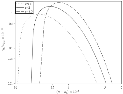
Figure 1.— Kinematic growth rate of parallel propagating Langmuir oscillations $\gamma_{p}(b=0)/\omega_{p,e}$ for the case of no perpendicular spread ($b=0$) and the dispersion relation $\omega_{R}/\omega_{p,e}$ as a function of normalized wavenumber $\kappa$ for $x_{c}=10^{6}$, $\beta_{e}=1.8\cdot 10^{-3}$ and $s=1.5,2,2.5$.

4.2. Maximum growth rate

Figure 2.— Plot of the function $C(A)$ for three values of $s=1.5,2,2.5$ as a function of $A$.

The function $C(A,s)$, defined in Eq. (61), is plotted in Fig. 2 for three values of $s=1.5,2,2.5$. It has one zero at $A_{N}(s)=s$, is negative for smaller $A<s$, and positive for larger $A>s$, in agreement with Eq. (57). Extrema are located at values of $A$ satisfying

$$A^{2}-(2s-1)A+s(s-2)=0$$ (66)

For values of $1<s\leq 2$ the function $C(A,s)$ attains its maximum value at

$$A_{0}(1<s\leq 2)={2s-1\over 2}\left[1+\sqrt{1+{s(2-s)\over(s-{1\over 2})^{2}}}\right]$$ (67)

For the special case $s=2$ we find $A_{N}(2)=2$ and $A_{0}(2)=3$ and the maximum value

$$C_{\rm max}(s=2)=e^{-3}$$ (68)

For values of $s>2$ the function $C(A,s)$ has a negative minimum at

$$A_{\rm min}(s>2)={2s-1\over 2}\left[1-\sqrt{1-{s(s-2)\over(s-{1\over 2})^{2}}}\right]$$ (69)

and a positive maximum at

$$A_{0}(s>2)={2s-1\over 2}\left[1+\sqrt{1-{s(s-2)\over(s-{1\over 2})^{2}}}\right]$$ (70)

It is straightforward to show that the location of the maximum $A_{0}(s)<A_{N}(s)$ is always above the location of the zero $A_{N}(s)$, in agreement with Fig. 2. In Table 1 we calculate the locations $A_{0}(s)$ and values of $C_{\rm max}(s)$ for different values of $s$.

Table 1Values of the zeros $A_{N}(s)=s$, location of maxima $A_{0}(s)$, maxima $C_{\rm max}(s)$ and minimum correction function $B(A_{0}(s),b=0.1,s)-1$ for different values of $s$ and $b=0.1$.

$s$	$A_{0}$	$C_{\rm max}(s)$	$B(A_{0}(s),b=0.1,s)-1$
1.5	2.32	$1.17\cdot 10^{-2}$	$-1.35\cdot 10^{-5}$
2.0	3.00	$4.98\cdot 10^{-2}$	$-2.25\cdot 10^{-5}$
2.5	3.66	$6.44\cdot 10^{-2}$	$-3.35\cdot 10^{-5}$
3.0	4.30	$7.58\cdot 10^{-2}$	$-4.62\cdot 10^{-5}$
4.0	5.56	$9.28\cdot 10^{-2}$	$-7.62\cdot 10^{-5}$

For ease of exposition we continue with the simplest case $s=2$. From Eq. (60) we then obtain for the maximum kinetic growth rate

$$\gamma_{p}^{\rm max}(b=0)={\gamma_{p}^{0}\kappa_{0}x_{c}\over e^{3}},$$ (71)

which occurs at $A_{0}=3$, corresponding to values of $K_{0}(R)=x_{c}/3$ and values of

$$R^{2}_{0}={1\over 1+{9\over x_{c}^{2}}}\simeq 1-{9\over x_{c}^{2}}$$ (72)

slightly below unity.

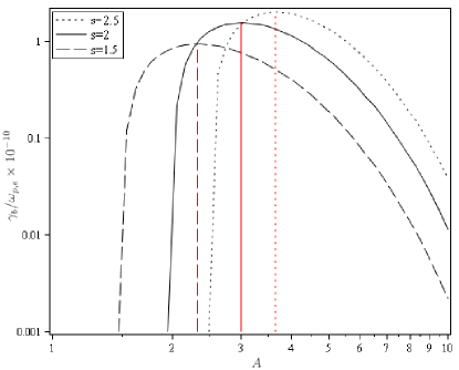
Figure 3.— Kinematic growth rate of parallel propagating Langmuir oscillations $\gamma_{p}(b=0)/\omega_{p,e}$ for the case of no perpendicular spread ($b=0$) as a function of the variable $A$ for $x_{c}=10^{6}$, $\beta_{e}=1.8\cdot 10^{-3}$ and $s=1.5,2,2.5$.

In Fig. 3 we show the growth rate from Fig.1 now as a function of the variable $A$. We note that the location of the maximum and the zero in the case $s=2$ agree exactly with the analytical values.

With the dispersion relation (52) and the definition (53) we find for the corresponding wavenumber

$$\kappa_{0}={1\over\sqrt{1-{3\beta_{e}^{2}\over 2}-{9\over x_{c}^{2}}}}\simeq 1+{3\beta_{e}^{2}\over 4}+{9\over 2x_{c}^{2}}\simeq 1$$ (73)

Maximum growth occurs at frequencies

$$\omega_{R,0}=\omega_{p,e}\kappa_{0}R_{0}\simeq\omega_{p,e},$$ (74)

in perfect agreement with the reactive result (24).

Moreover, the maximum growth rate (71) is given by

$$\gamma_{p}^{\rm max}(b=0)=2.8\cdot 10^{-9}{n_{22}x_{c,6}\over N_{7}^{1/2}}\;\;\hbox{Hz}$$ (75)

which is about an order of magnitude larger than the maximum reactive growth rate (25). Apparently, the spread in parallel momentum of the pair distribution function does not reduce the maximum growth rate of parallel Langmuir oscillations, in disagreement with the result of Miniati and Elyiv (2013).

At the same values of $R_{0}$ and $\kappa_{0}$, because of the exponential factor, the Landau damping rate (63) of Langmuir oscillations is negligibly small

$$\gamma_{L}(R_{0})=\pi^{1/2}\omega_{p,e}\kappa_{0}R_{0}\left({R_{0}\over\beta_{e}}\right)^{3}e^{-{R_{0}^{2}\over\beta_{e}^{2}}}$$

$$\simeq{\pi^{1/2}\omega_{p,e}\over\beta_{e}^{3}}e^{-{1\over\beta_{e}^{2}}}<10^{-10^{5}}$$ (76)

5. Kinetic instability analysis of Langmuir oscillations for finite perpendicular spread

With the correction function (45) for finite perpendicular spreads below the limit $b_{0}$, the growth rate in this case

$$\gamma_{p}(b)=B(X)\gamma_{p}(b=0)$$ (77)

is simply related to the growth rate $\gamma_{p}(b=0)$. The growth rate $\gamma_{p}(b)$ with finite spread as compared to the growth rate $\gamma_{p}(b=0)$ with no finite spread is enhanced (reduced) if the correction function (45) is greater (smaller) than unity. The correction function (45) reads

$$B(X)=B(A,b,s)={e^{X^{2}}\over X}\left[(1+h)F(X)-hX\right]$$ (78)

with the function

$$h(A,s)={(s-1)A-s(s-2)\over 2A(A-s)}$$ (79)

We noted before that the growth rate $\gamma_{p}(b=0)$ is positive only for values of $A>s$, so we restrict our analysis to this range. For $A>s$ the function (79) is positive for all values of $A>s>1$. With $A=s+t$ the function (79) reads

$$h(t,s)={s+(s-1)t\over 2t(t+s)}={s-1\over 2(t+s)}+{s\over 2t(t+s)}$$ (80)

with $t\in(0,\infty]$. The function is strictly decreasing, as

$${dh(t,s)\over dt}=-{(s-1)t^{2}+2st+s^{2}\over 2t^{2}(t+s)^{2}}$$ (81)

is always negative. No extreme values occur in the interval $(0,\infty]$. For later use we note that the condition $h(A,s)=1/2$ leads to the equation

$$A^{2}-(2s-1)A+s(s-2)=0,$$ (82)

which is identical to Eq. (66), determining the maximum growth rate $\gamma^{\rm max}_{p}(b=0)$ through the function $C(A,s)$. Hence, at the maximum $A_{0}(s)$ the function

$$h(A_{0}(s),s)={1\over 2}$$ (83)

for all values of $s$. Moreover, for larger values of $A>A_{0}(s)$, the function $h(A,s)<1/2$.

5.1. Correction function for the maximum growth rate

The maximum growth rate $\gamma_{p}^{\rm max}(b=0)$ occurs at $A_{0}(s)$ listed in Table 1. For values of $b<0.1$ the variable (44)

$$X=\sqrt{A_{0}(s)\over 2}b<0.071\sqrt{A_{0}(s)}<0.17$$ (84)

is smaller than unity for all values of $b<0.1$, because for $s\leq 4$ we calculated $A_{0}(s)\leq A_{0}(4)=5.56$. We therefore use the series expansion (106) for Dawson’s integral in Eq. (78) to find

$$B(X\ll 1)\simeq e^{X^{2}}\left[1-{2\over 3}(1+h)X^{2}(1-{2\over 5}X^{2})\right]$$

$$\simeq 1-{2h-1\over 3}X^{2}-{4h-1\over 10}X^{4},$$ (85)

With the value (83) the quadratic terms vanishes and we obtain the correction

$$B(A_{0}(s),b,s)\simeq 1-{X^{4}\over 10}=1-{A^{2}_{0}(s)b^{4}\over 40}$$ (86)

For the maximum value of $b=0.1$, we calculate the reduction factor $B(A_{0}(s),b,s)-1$ for different values of $s$. The results are listed in Table 1. As can be seen, the reduction factors due to the finite spread in the pair distribution function are tiny, always less than $(-10^{-4})$. Contrary to the statement of Miniati and Elyiv (2013) we find that the finite perpendicular spread does not significantly reduce the maximum growth rate.

5.2. General behavior of the correction function

Dawson’s integral satisfies the linear differential equation

$${dF(X)\over dX}=1-2XF(X),$$ (87)

so that the first derivative of the correction function (78) is given by

$${\partial B(X)\over\partial X}={e^{X^{2}}\over X^{2}}\left[(1+h)X-(1+h)F(X)-2hX^{3}\right]$$ (88)

The extreme value of the correction function $B(X_{E})$ occurs at $X_{E}$ given by the solution of the transcendental equation

$$X_{E}-F(X_{E})={2h\over 1+h}X_{E}^{3}$$ (89)

Inserting this condition into Eq. (78) we obtain for the extreme value of the correction function

$$B_{E}=e^{X_{E}^{2}}\left[1-2hX_{E}^{2}\right]$$ (90)

We recall that for values of $A>A_{0}(s)$, corresponding to $X_{E}>b\sqrt{A_{0}(s)/2}$, the function $h<1/2$. The first and second derivative of function (90) are given by

$${dB_{E}\over dX_{E}}=2X_{E}e^{X_{E}^{2}}\left[(1-2h)-2hX_{E}^{2}\right]$$ (91)

and

$${d^{2}B_{E}\over dX^{2}_{E}}=2e^{X_{E}^{2}}\left[(1-2h)+2(1-5h)X_{E}^{2}-4hX_{E}^{4}\right]$$ (92)

The function $B_{E}$ has a single maximum at $X^{2}_{E}=(1-2h)/2h$ given by

$$B_{E}^{\rm max}=2he^{{1\over 2h}-1}$$ (93)

For given $b$, Eq. (90) corresponds to the extreme value

$$B_{E}(A_{E})=e^{b^{2}A_{E}\over 2}\left[1-hb^{2}A_{E}\right]$$

$$=e^{b^{2}A_{E}\over 2}\left[1-{b^{2}\over 2}\left(s-1-{s\over A_{E}-s}\right)\right],$$ (94)

where we inserted the function $h(A_{E},s)$ from Eq. (79). Even without knowing the value $A_{E}$, we can draw some interesting conclusions from Eq. (94).

For values of $s\ll A_{E}\ll(2/b^{2})$ the function (94) approaches

$$B_{E}(s\ll A_{E}\ll{2\over b^{2}})\simeq 1-{b^{2}(s-1)\over 2},$$ (95)

producing at most a tiny correction over a wide range of $s\ll A_{e}\ll 200$ in agreement with our earlier discussion of the maximum growth rate.

6. Summary and conclusions

The interaction of TeV gamma rays from distant blazars with the extragalactic background light produces relativistic electron-positron pair beams by the photon-photon annihilation process. The created pair beam distribution is unstable to linear two-stream instabilities of both electrostatic and electromagnetic nature in the unmagnetized intergalactic medium. Based on a linear reactive instability analysis Broderick et al. (2012) and Schlickeiser et al. (2012) have concluded that the created pair beam distribution function is quickly unstable to the excitation of electrostatic oscillations in the unmagnetized intergalactic medium, so that the generation of inverse-Compton scattered GeV gamma-ray photons by the pair beam is significantly suppressed. Because most of the pair kinetic energy is transferred to electrostatic fluctuations, less kinetic pair energy is available for inverse Compton interactions with the microwave background radiation fields. Therefore, there is no need to require the existence of small intergalactic magnetic fields to scatter the produced pairs, so that the explanation (made by several authors) of the FERMI non-detection of the inverse Compton scattered GeV gamma rays by a finite deflecting intergalactic magnetic field is not necessary. In particular, the various derived lower bounds for the intergalactic magnetic fields are invalid due to the pair beam instability argument.

Miniati and Elyiv (2013) have argued that the more appropriate linear kinetic instability analysis, accounting for the longitudinal and the small but finite perpendicular momentum spread in the pair momentum distribution function, significantly reduces the growth rate of electrostatic oscillations by orders of magnitude compared to the linear reactive instability analysis, concluding that the pair beam instability does not modify the pair cascade as in vacuum. We therefore have repeated the linear instability analysis in the kinetic limit for parallel propagating electrostatic oscillations using the realistic pair distribution function with longitudinal and perpendicular spread. Contrary to the claims of Miniati and Elyiv (2013) we find that neither the longitudinal nor the perpendicular spread in the relativistic pair distribution function do significantly affect the electrostatic growth rates. The maximum kinetic growth rate for no perpendicular spread is even about an order of magnitude greater than the corresponding reactive maximum growth rate. The reduction factors to the maximum growth rate due to the finite perpendicular spread in the pair distribution function are tiny, and always less than $10^{-4}$. We confirm the earlier conclusions by Broderick et al. (2012) and Schlickeiser et al. (2012a), that the created pair beam distribution function is quickly unstable in the unmagnetized intergalactic medium.

As our analysis has shown, relativistic kinetic instability studies are notoriously difficult and complicated due to plasma particle velocities close to the speed of light. Therefore extreme care is necessary in order to include all relevant relativistic effects, as done in the present study.

7. Appendix A: Approximations of the integral $J(b)$

We introduce

$$T(b,A,s)={K^{s+1}(R)\over A}e^{A}bJ(b),$$ (96)

so that according to Eqs. (40)

$$T(b,A,s)=e^{A}\int_{0}^{b}dq\,{e^{-{A\over\sqrt{1+q^{2}}}}\over(1+q^{2})^{s+1\over 2}}\left[1-{s\over A}\sqrt{1+q^{2}}\right]$$ (97)

The substitution $q=\tan t$ provides

$$T(b,A,s)=e^{A}\Bigl{[}\int_{0}^{\hbox{arctan}\,b}dt\,\cos^{s-1}t\,e^{-A\cos t}$$

$$-{s\over A}\int_{0}^{\hbox{arctan}\,b}dt\,\cos^{s-2}t\,e^{-A\cos t}\Bigr{]}$$

$$=Y(b,A,p={s-1\over 2})-{s\over A}Y(b,A,p={s-2\over 2})$$ (98)

with

$$Y(b,A,p)=e^{A}\int_{0}^{\hbox{arctan}\,b}dt\,\cos^{2p}t\,e^{-A\cos t}$$ (99)

Because $b$ is significantly smaller than unity, we approximate

$$\cos t\simeq 1-{t^{2}\over 2},$$ (100)

so that with $\hbox{arctan}\,b\simeq b$

$$Y(b,A,p)\simeq\int_{0}^{b}dq\,[1-pq^{2}]e^{{Aq^{2}\over 2}}$$ (101)

We restrict our analysis to values of $\beta_{e}\leq R\ll R_{0}$, where $R_{0}$ denotes the real phase speed (72), where the maximum growth rate $\gamma^{\rm max}_{p}(b=0)$ for no angular spread occurs (see Sect. 4.2). In this case the variable (41)

$$A(R\leq R_{0})\geq A(R_{0})>3$$ (102)

is always larger than $3$. The main contribution to the integral (101) is then indeed provided by small values of $q\ll 1$, so that the approximation (100) is justified.

The integral (101) can be expressed in terms of Dawson’s integral (Abramowitz and Stegun 1972, Ch. 7.1; Lebedev 1972, Ch. 2.3), the error function of imaginary argument,

$$F(x)=e^{-x^{2}}\int_{0}^{x}dt\,e^{t^{2}}$$ (103)

as

$$Y(b,A,p)=\sqrt{2\over A}e^{X^{2}}\bigl{[}F\left(X\right)+{p\over A}[F\left(X\right)-X]\bigr{]},$$ (104)

with

$$X(b,A)=\sqrt{A\over 2}b$$ (105)

Dawson’s integral (103) has a maximum $F_{m}=0.541$ at $x_{m}=0.924$, the series expansion

$$F(x)=\sum_{n=0}^{\infty}{(-1)^{n}2^{n}x^{2n+1}\over 1\cdot 3\cdot\cdot\cdot(2n+1)}=x\left[1-{2\over 3}x^{2}+{4\over 15}x^{4}\mp\ldots\right]$$ (106)

and the asymptotic expansion

$$F(x\gg 1)\simeq{1\over 2x}[1+{1\over 2x^{2}}+{3\over 4x^{4}}]$$ (107)

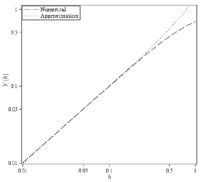
Figure 4.— Comparison of the numerically evaluated exact integral (99) with its approximation (104) for $p=2$ and $A=3$.

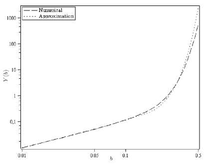
Figure 5.— Comparison of the numerically evaluated exact integral (99) with its approximation (104) for $p=2$ and $A=100$.

In Figures 4 and 5 we compare the numerically evaluated exact integral (99) with its approximation (104) for $p=2$ and two values of $A=3$ and $A=100$. In both cases the agreement is excellent for values of $b<0.1$.

According to Eqs. (96) and (98) we obtain the approximations

$$J(b)\simeq{Ae^{-A}\over K^{s+1}(R)}{e^{X^{2}}\over X}\Bigl{[}(1-{s\over A})F(X)$$

$$+\left((s-1)A-s(s-2)\right){F(X)-X\over 2A^{2}}\Bigr{]}$$ (108)

The small argument expansion (106) readily yields

$$J(0)=J(b=0)={A-s\over K^{s+1}(R)}e^{-A},$$ (109)

which agrees with Eq. (42), so that the correction function (45) becomes

$$B(X)={e^{X^{2}}\over X}\left[F(X)+h(A,s)(F(X)-X)\right],$$ (110)

with

$$h(A,s)={(s-1)A-s(s-2)\over 2A(A-s)}$$ (111)

8. Appendix B: Collective electrostatic modes

Eq. (47) together with the real part of the dispersion relation (37) reads

$$0=\Re\Lambda(R,I=0)=1-$$

$${1\over\kappa^{2}\beta_{e}^{2}}\left[\Re Z^{{}^{\prime}}\left({R\over\beta_{e}}\right)+{1\over\chi}\Re Z^{{}^{\prime}}\left({R\over\sqrt{\chi\xi}\beta_{e}}\right)\right]$$ (112)

In order to use the asymptotic expansions (28) for proton-electron temperature ratios $\chi<\xi^{-1}=1836$ we have to consider three cases:

(a) In the case of phase speeds larger than $\beta_{e}$,

$$R\gg\beta_{e}.$$ (113)

both arguments of the $Z^{{}^{\prime}}$-function are large compared to unity, so that we may use the asymptotic expansion

$$\Re Z^{{}^{\prime}}(t\gg 1)\simeq{1\over t^{2}}[1+{3\over 2t^{2}}]$$ (114)

(b) In the case of intermediate phase speeds,

$${R\over\beta_{e}}\ll 1\ll{R\over\sqrt{\chi\xi}\beta_{e}},$$ (115)

we use the expansion (114) in the third term of Eq. (112) and the asymptotic expansion for small arguments

$$\Re Z^{{}^{\prime}}(t\ll 1)\simeq-2[1-2t^{2}]$$ (116)

in the second term of Eq. (112).

(c) In the case of very small phase speeds,

$$R\ll\sqrt{\chi\xi}\beta_{e},$$ (117)

we use the expansion (116) in the second and third term of Eq. (112).

We consider each case in turn.

8.1. Large phase speed $R\gg\beta_{e}$

Here we readily obtain for Eq. (112)

$$\Re\Lambda(R,\kappa)=1-{1+\xi\over\kappa^{2}R^{2}}-{3\beta_{e}^{2}(1+\chi\xi^{2})\over 2\kappa^{2}R^{4}}=0$$ (118)

yielding the dispersion relation

$$R^{4}-{1+\xi\over\kappa^{2}}R^{2}-{3\beta_{e}^{2}\over 2\kappa^{2}}=0$$ (119)

with the solution

$$R^{2}={1+\xi\over 2\kappa^{2}}\left[1+\sqrt{1+{6\beta_{e}^{2}\kappa^{2}\over(1+\xi)^{2}}}\right]\simeq{1\over 2\kappa^{2}}\left[1+\sqrt{1+{6\beta_{e}^{2}\kappa^{2}}}\right]$$ (120)

The requirement $R\gg\beta_{e}$ implies the wavenumber restriction $\beta_{e}^{2}\kappa^{2}\ll 2.5$. Likewise, the subluminality requirement $R<1$ demands

$$\kappa^{2}>\kappa_{L}^{2}=1+{3\beta_{e}^{2}\over 2}$$ (121)

In this wavenumber range the solution (119) reduces to

$$R^{2}\simeq{1\over\kappa^{2}}+{3\beta_{e}^{2}\over 2}={1+{3\over 2}\beta_{e}^{2}\kappa^{2}\over\kappa^{2}},$$ (122)

corresponding to Langmuir oscillations

$$\omega_{R}^{2}=\omega_{p,e}^{2}[1+3k^{2}\lambda_{De}^{2}]$$ (123)

for $2^{-1/2}\beta_{e}\leq k\lambda_{De}\ll 1$ with the electron Debye length $\lambda_{De}=\beta_{e}c/\sqrt{2}\omega_{p,e}$.

8.2. Intermediate phase speed $\sqrt{\chi\xi}\beta_{e}=\beta_{p}\ll R\ll\beta_{e}$

In this case we derive for Eq. (112)

$$\Re\Lambda(R,\kappa)\simeq 1+{2\over\beta_{e}^{2}\kappa^{2}}-{\xi\over\kappa^{2}R^{2}}-{4R^{2}\over\beta_{e}^{4}\kappa^{2}}=0,$$ (124)

yielding the dispersion relation

$$R^{4}-{\beta_{e}^{2}\over 2}(1+{\beta_{e}^{2}\kappa^{2}\over 2})R^{2}+{\xi\beta_{e}^{4}\over 4}=0$$ (125)

with the two formal solutions

$$R^{2}_{1,2}={\beta_{e}^{2}\over 4}(1+{\beta_{e}^{2}\kappa^{2}\over 2})\left[1\pm\sqrt{1-{4\xi\over(1+{\beta_{e}^{2}\kappa^{2}\over 2})^{2}}}\right]$$

$$\simeq{\beta_{e}^{2}\over 2}(1+{\beta_{e}^{2}\kappa^{2}\over 2})\left[1\pm\left(1+{\xi\over(1+{\beta_{e}^{2}\kappa^{2}\over 2})^{2}}\right)\right]$$ (126)

The first solution

$$R^{2}_{1}\simeq\beta_{e}^{2}(1+{\beta_{e}^{2}\kappa^{2}\over 2})$$ (127)

violates the restriction $R^{2}\ll\beta_{e}^{2}$, leaving as only solution

$$R^{2}=R_{2}^{2}\simeq{{\xi\beta_{e}^{2}\over 2}\over 1+{\beta_{e}^{2}\kappa^{2}\over 2}}$$ (128)

This ion sound wave solution has to fulfill the second restriction $R^{2}\gg\chi\xi\beta_{e}^{2}$, corresponding to the condition

$$1+{\beta_{e}^{2}\kappa^{2}\over 2}\ll{1\over 2\chi},$$ (129)

which is only possible for values of $\chi\ll 1$ or $T_{p}\ll T_{e}$. In this case the solution (128) holds for wavenumbers $\kappa^{2}\beta_{e}^{2}\ll\chi^{-1}$. Therefore the ion sound wave solution only exists for $T_{p}\ll T_{e}$ at wavenumbers $(\lambda_{De}k)^{2}\ll(2\chi)^{-1}$ with frequencies

$$\omega_{R}^{2}={\beta_{p}^{2}c^{2}k^{2}\over 2(1+\lambda^{2}_{De}k^{2})},\,\;\;\lambda^{2}_{De}k^{2}\ll{1\over 2\chi}={T_{e}\over 2T_{p}}$$ (130)

8.3. Very small phase speed $R\ll\sqrt{\chi\xi}\beta_{e}=\beta_{p}$

In this case we derive for Eq. (112)

$$\Re\Lambda(R,\kappa)\simeq 1+{2(1+\chi)\over\chi\beta_{e}^{2}\kappa^{2}}-{4(1+\xi\chi^{2})R^{2}\over\xi\chi^{2}\beta_{e}^{4}\kappa^{2}}=0,$$ (131)

yielding the dispersion relation

$$R^{2}={(1+\chi)\chi\xi\beta_{e}^{2}\over 2(1+\xi\chi^{2})}+{\xi\chi^{2}\beta_{e}^{4}\kappa^{2}\over 4(1+\xi\chi^{2})}$$ (132)

The very small phase speed requirement $R^{2}\ll\chi\xi\beta_{e}^{2}$ corresponds to

$${(1+\chi)\over 2(1+\xi\chi^{2})}+{\chi\beta_{e}^{2}\kappa^{2}\over 4(1+\xi\chi^{2})}\ll 1,$$ (133)

which cannot be fulfilled. Therefore no electrostatic mode with very small phase speeds exists.

References

- a (1972) Abramowitz, M., Stegun, I. A., 1972, Handbook of Mathematical Functions, NBS, Washington
- b (2012) Broderick, A. E., Chang, P., Pfrommer, C., 2012, ApJ 732, 22
- c (2012) Cairns, I. H., 1989, Phys. Fluids B 1, 204
- d (2012) Dermer, C. D., Cavadini, M., Razzaque, S., Finke, J. D., Chiang, J., Lott, B., 2011, ApJ 733, L21
- e (2012) Dolag, K., Kachelriess, M., Ostrapchenko, S., Tomas, R., 2011, ApJ 727, L4
- f (2012) Elyiv, A., Neronov, A., Semikoz, D. V., 2009, Phys. Rev. D 80, 023010
- g (2012) Fried, B. D., Conte, S. D., 1961, The Plasma Dispersion Function, Academic Press, New York
- h (2012) Hui,L., Gnedin, N. Y., 1997, MNRAS 292, 27
- i (2012) Hui,L., Haiman, Z., 2003, ApJ 596, 9
- j (2012) Lebedev, N. N., 1972, Special Functions and their applications, Dover, New York
- k (2012) Miniati, F., Elyiv, A., 2013, ApJ 770, 54
- l (2012) Neronov, A., Vovk, I., 2010, Science 328, 73
- m (2012) Schlickeiser, R., 2002, Cosmic Ray Astrophysics, Springer, Berlin
- n (2012) Schlickeiser, R., 2010, Phys. Plasmas 17, 112105
- o (2012) Schlickeiser, R., Elyiv, A., Ibscher, D., Miniati, F., 2012b, ApJ 758, 101
- p (2012) Schlickeiser, R., Ibscher, D., Supsar, M., 2012a, ApJ 758, 102
- q (2012) Schlickeiser, R., Yoon, P. H., 2012, Phys. Plasmas 19, 022105
- r (2012) Takahashi, K., Mori, M., Ichiki, K., Inoue, S., Takami, H., 2012, ApJ 744, L42
- s (2012) Tavecchio, F., Ghisellini, G., Bonnoli, G., Foschini, L., 2011, MNRAS, 414, 3566
- t (2012) Taylor, A. M., Vovk, I., Neronov, A., 2011, A & A 529, A144
- v (2012) Vovk, I., Taylor, A. M., Semikoz, D. V., Neronov, A., 2012, ApJ 747, L14