Electron transport through a quantum dot assisted by cavity photons

Abstract

We investigate transient transport of electrons through a single-quantum-dot controlled by a plunger gate. The dot is embedded in a finite wire that is weakly coupled to leads and strongly coupled to a single cavity photon mode. A non-Markovian density-matrix formalism is employed to take into account the full electron-photon interaction in the transient regime. In the absence of a photon cavity, a resonant current peak can be found by tuning the plunger gate voltage to lift a many-body state of the system into the source-drain bias window. In the presence of an $x$-polarized photon field, additional side peaks can be found due to photon-assisted transport. By appropriately tuning the plunger-gate voltage, the electrons in the left lead are allowed to make coherent inelastic scattering to a two-photon state above the bias window if initially one photon was present in the cavity. However, this photon-assisted feature is suppressed in the case of a $y$-polarized photon field due to the anisotropy of our system caused by its geometry.

I Introduction

Electronic transport through quantum dot (QD) related systems has received tremendous attention in recent years due to its potential application in various fields, such as implementation of quantum computing,Nakamura et al. (1999) nanoelectromechanical systems,Villavicencio et al. (2008) photodetectors,van Kouwen et al. (2010) and biological sensors.Jin et al. (2011) The QD embedded structure can be fabricated in a two-dimensional electron gas, controlled by a plunger-gate voltage, and connected to the leads by applying an external source-drain bias voltage.

The electronic transport under the influence of time-varying external fields is one of the interesting areas. The transport phenomena in the presence of photons have been intensively studied in many mesoscopic systems. Pedersen and Büttiker (1998); Stoof and Nazarov (1996); Foa Torres (2005); Kouwenhoven et al. (1994a); Niu and Lin (1997); Hu (1993); Tang and Chu (2000); Wätzel et al. (2011); Shibata et al. (2012); Ishibashi and Aoyagi (2002) Various quantum confined geometries to characterize the photon-assisted features are for example a quantum ring with an embedded dot for exploring mono-parametric quantum charge pumping, Foa Torres (2005) a single QD for investigating the single-electron (SE) tunneling, Kouwenhoven et al. (1994a) a quantum wire for studying the electron population inversion, Niu and Lin (1997) and a quantum point contact involving photon-induced intersubband transitions. Hu (1993); Tang and Chu (2000) Recently, electrical properties of double QD systems influenced by electromagnetic irradiation have been studied,Wätzel et al. (2011); Shibata et al. (2012) pointing out spin-filtering effect,Wätzel et al. (2011) and two types of photon-assisted tunneling related to the ground state and excited state resonances. Shibata et al. (2012) The classical and quantum response was investigated experimentally in terms of the sharpness of the transition rate which depends on the thermal broadening of the Fermi level in the electrodes and the broadening of the confined levels. Ishibashi and Aoyagi (2002)

In the above mentioned examples the photon-assisted transport was induced by a classical electromagnetic field. It is also interesting to investigate electronic transport through a QD system influenced by quantized photon field. A single-photon source is an essential building block for the manipulation of the quantum information coded by a quantum state.Imamoglu and Yamamoto (1994) This issue has been considered by calculating resonant current carried by negatively charged excitons through a double QD system confined in a cavity,Joshi et al. (2011) where resonant tunneling between two QDs is assisted by a single photon. However, modeling of transient electronic transport through a QD in a photon cavity is still in its infancy.

To study time-dependent transport phenomena in mesoscopic systems, a number of approaches have been employed. In closed systems, the Jarzynski equation was derived by defining the free-energy difference of the system between the initial and final equilibrium state in terms of stochastic Liouville equationMukamel (2003) or microscopic reversibility. Monnai (2005) In open quantum systems where the system is connected to electron reservoirs, the Jarzynski equation can be derived using a master equation approach to investigate fluctuation theorems Esposito and Mukamel (2006) and dissipative quantum dynamics. Crooks (2008) In order to investigate interaction effects on the transport behavior, several approaches have been proposed based on the quantum master equation (QME) applied to a quantum measurement of a two-state system, Rammer et al. (2004) calculation of current noise spectrum, Luo et al. (2007) and the counting statistics of electron transfers through a double QD. Welack et al. (2008) The QME describes the evolution of the reduced density (RD) operator caused by the Hamiltonian of the closed system in the presence of the electron or photon reservoirs. Thus, the QME usually consists of two parts, a part describing the unitary evolution of the closed system, and a dissipative part describing the influence of the reservoirs. Lambropoulos et al. (2000)

In an open current-carrying system weakly coupled to leads, the master equations within the Markovian and wide-band approximations have been commonly derived and used.Van Kampen (2001); Harbola et al. (2006); Gurvitz and Prager (1996) The coupling to electron or photon reservoirs can be considered to be Markovian and the rotating wave approximation are often used for the electron-photon coupling.Van Kampen (2001) The QME may reduce to a “birth and death master equation” for populations,Harbola et al. (2006) or modified rate equations. Gurvitz and Prager (1996) The energy dependence of the electron tunneling rate or the memory effect in the system are usually neglected.

The non-Markovian density-matrix formalism with energy-dependent coupling elements should be considered to study the full counting statistics for electronic transport through interacting electron systems. Braggio et al. (2006); Emary et al. (2007); Bednorz and Belzig (2008) It was noticed that the Markovian limit neglects coherent oscillations in the transient regime, and the rate at which the steady state is reached does not agree with the non-Markovian model.Vaz and Kyriakidis (2010) The Markov approximation shows significantly longer time to reach a steady state when the tunneling anisotropy is high, thus confirming its applicability only in the long-time limit. To investigate the transient transport, a non-Markovian density-matrix formalism involving energy-dependent coupling elements should be explicitly considered.Gudmundsson et al. (2009)

The aim of this work is to investigate how the $x$- and $y$-polarized single photon mode influence the ballistic transient electronic transport through a QD embedded in a finite quantum wire in a uniform perpendicular magnetic field based on the non-Markovian dynamics. We explicitly build a transfer Hamiltonian that describes the contact between the central quantum system and semi-infinite leads with a switching-on coupling in a certain energy range. By controlling the plunger gate, we shall demonstrate robust photon-assisted electronic transport features when the physical parameters of the single-photon mode are appropriately tuned to cooperate with the electron-photon coupling and the energy levels of the Coulomb interacting electron system.

The paper is organized as follows. In Sec. II, we model a QD with interacting electrons embedded in a quantum wire coupled to a single-photon mode in a uniform magnetic field, in which the full electron-photon coupling is considered. The transient dynamics is calculated using a generalized QME based on a non-Markovian formalism. Section III demonstrates the numerical results and transient transport properties of the plunger-gate controlled electron system coupled to the single-photon mode with either $x$- or $y$-polarization. Concluding remarks will be presented in Sec. IV.

II Model and Theory

In this section, we describe how the embedded QD, realized in a two-dimensional electron gas in gallium arsenide (GaAs), can be described by the potential $V_{\rm QD}$ in a finite quantum wire and its connection to the leads in a uniform perpendicular magnetic field. The plunger-gate controlled central electronic system is strongly coupled to a single photon mode that can be described by a many-body (MB) system Hamiltonian $H_{\rm S}$, in which the electron-electron interaction and the electron-photon coupling to the $x$- and $y$-polarized photon fields are explicitly taken into account, as is depicted in Fig. 1(a). A generalized QME is numerically solved to investigate the dynamical transient transport of electrons through the single QD system.

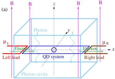
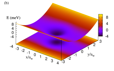
Figure 1: (Color online) (a) Schematic of a QD embedded in a quantum wire coupled to a photon cavity, connected to the left lead (red) with chemical potential $\mu_{\rm L}$, and the right lead (brown) with chemical potential $\mu_{\rm R}$ in an external magnetic field $B$. (b) Schematic diagram depicts the potential representing the QD embedded in a quantum wire with parameters $B=0.1~{}{\rm T}$, $a_{w}=23.8~{}{\rm nm}$, and $\hbar\Omega_{0}=2.0~{}{\rm meV}$.

II.1 QD-embedded wire in magnetic field

The electron system under investigation is a two-dimensional finite quantum wire that is hard-wall confined at $x$ = $\pm L_{x}/2$ in the $x$-direction, and parabolically confinement in the $y$-direction. The system is exposed to an external perpendicular magnetic field ${\bf B}=B\hat{z}$ defining a magnetic length $l=(h/eB)^{1/2}=25.67[B({\rm T})]^{-1/2}$ nm, and the effective confinement frequency $\Omega^{2}_{w}=\omega^{2}_{c}+\Omega^{2}_{0}$ being expressed in the cyclotron frequency $\omega_{c}=eB/m^{*}c$ as well as in the bare confinement energy $\hbar\Omega_{0}$ characterizing the transverse electron confinement. The system is scaled by the effective magnetic length $a_{w}=(\hbar/m^{*}\Omega_{w})^{1/2}$. Figure 1(b) shows the embedded QD subsystem scaled by $a_{w}$, where the QD potential is considered of a symmetric Gaussian shape

$$V_{\rm QD}(x,y)=V_{0}\;\exp{\left[-\beta_{0}^{2}\left(x^{2}+y^{2}\right)\right]}$$ (1)

with strength $V_{0}=-3.3$ meV and $\beta_{0}$ = $3.0\times 10^{-2}~{}{\rm nm^{-1}}$ such that the radius of the QD is $R_{\rm QD}\approx 33.3~{}{\rm nm}$.

II.2 Many-Body Model

In this section, we describe how to build up the time-dependent Hamiltonian $H(t)$ of an open system that couples the QD-embedded MB system to the leads. The Coulomb and photon interacting electrons of the QD system are described by a MB system Hamiltonian $H_{\rm S}$. In the closed electron-photon interacting system, the MB-space $\{|\breve{\nu})\}$ is constructed from the tensor product of the electron-electron interacting many-electron (ME) state basis $|\nu)$ and the eigenstates $|N\rangle$ of the photon number operator $a^{{\dagger}}a$, namely $|\breve{\nu})=|\nu)\otimes|N\rangle$. Jonasson et al. (2012) The Coulomb interacting ME states of the isolated system are constructed from the SE states.Abdullah et al. (2010) The time-dependent Hamiltonian describing the MB system coupled to the leads

$$H(t)=H_{\mathrm{S}}+\sum_{l=\mathrm{L,R}}\left[H_{l}+H_{\mathrm{T}l}(t)\right]$$ (2)

consists of a disconnected MB system Hamiltonian $H_{\mathrm{S}}$, and ME Hamiltonian of the leads $H_{l}$ where the electron-electron interaction is neglected. In addition, $L$ and $R$ refer to the left and the right lead, respectively. Moreover, $H_{\mathrm{T}l}(t)$ is a time-dependent transfer Hamiltonian that describes the coupling between the QD system and the leads.

The isolated QD system including the electron-electron and the photon-electron interactions is governed by the MB system Hamiltonian

$$H_{\textrm{S}} = \sum_{i,j}\langle\psi_{i}\lvert\frac{\bm{\pi}^{2}}{2m^{*}}+V_{\mathrm{QD}}+eV_{\mathrm{pg}}\lvert\psi_{j}\rangle d_{i}^{\dagger}d_{j}$$ (3)

$$+H_{\textrm{e-e}}+H_{\rm ph}+H_{\rm Z}$$

where $|\psi\rangle$ is a SE state, $d^{\dagger}_{i}$ ($d_{j}$) are the electron creation (annihilation) operators in the central system, and $H_{\rm ph}=\hbar\omega_{\textrm{ph}}a^{\dagger}a$ is the photon Hamiltonian. In addition, $\bm{\pi}=\bm{\pi}_{e}+\frac{e}{c}\mathbf{A}_{\rm ph}$ where $\bm{\pi}_{e}=p+\frac{e}{c}\mathbf{A}_{\mathrm{ext}}$ is composed of the momentum operator $p$ of the electronic system and the vector potential $\mathbf{A}_{\mathrm{ext}}$ = ($0,-By,0$) represented in the Landau gauge. $H_{\rm Z}$ is the Zeeman energy $\pm\frac{1}{2}g^{\ast}\mu_{B}B$, where $\mu_{B}$ is the Bohr magneton and $g^{\ast}$ the effective Lande $g$-factor for the material.

In the Coulomb gauge, the photon vector potential can be represented as

$$\mathbf{A_{\rm ph}}=A_{\rm ph}\left(a+a^{\dagger}\right)\mathbf{\hat{e}}\,,$$ (4)

if the wavelength of the cavity mode is much larger than the size of the central system. Herein, $A_{\rm ph}$ is the amplitude of the photon field. The electron-photon coupling strength is thus defined by $g_{\rm ph}=eA_{\rm ph}\Omega_{w}a_{w}/c$. In addition, $\mathbf{\hat{e}}=(e_{x},0)$ indicates the electric field is polarized parallel to the transport direction in a TE₀₁₁ mode, and $\mathbf{\hat{e}}=(0,e_{y})$ denotes the electric field is polarized perpendicular to the transport direction in a TE₁₀₁ mode. Moreover, we introduce the plunger gate voltage $V_{\rm pg}$ to control the alignment of quantized energy levels in the QD system relative to the electrochemical potentials in the leads. In the second term of Eq. (3), $\hbar\omega_{\mathrm{ph}}$ is the quantized photon energy, and $a^{\dagger}(a)$ are the operators of photon creation (annihilation), respectively. The last term $H_{\textrm{e-e}}$ describes the electron-electron interaction.

In a second quantized form, the isolated MB system Hamiltonian $H_{\rm S}$ can be separated as

$$H_{\textrm{S}}=H_{\textrm{e}}+H_{\textrm{ph}}+H_{\textrm{e-ph}}+H_{\textrm{Z}}\,.$$ (5)

The first part of $H_{\rm S}$ is the Coulomb interacting electron Hamiltonian

$$H_{\textrm{e}}=\sum_{i}\left(E_{i}+eV_{\mathrm{pg}}\right)d_{i}^{\dagger}d_{i}+\frac{1}{2}\sum_{ijrs}\langle V_{\textrm{Coul}}\rangle d_{i}^{\dagger}d_{j}^{\dagger}d_{s}d_{r}\,,$$ (6)

where $E_{i}$ is the energy of a SE state, $V_{\mathrm{pg}}$ is the electrostatic potential of the plunger gate, and

$$\langle V_{\mathrm{Coul}}\rangle=\langle ij|V_{\mathrm{Coul}}|rs\rangle$$ (7)

$$= \int d\mathbf{r}d\mathbf{r^{\prime}}\psi^{\mathrm{S}}_{i}({\bf r})^{*}\psi^{\mathrm{S}}_{j}({\bf r}^{\prime})^{*}V({\bf r}-{\bf r}^{\prime})\psi^{\mathrm{S}}_{r}({\bf r}^{\prime})\psi^{\mathrm{S}}_{s}({\bf r})$$

are the Coulomb matrix elements in the SE state basis with $\psi^{\textrm{S}}({\bf r})$ being the SE state wavefunctions and the Coulomb interaction potential $V({\bf r}-{\bf r}^{\prime})$.Abdullah et al. (2010) The second part in Eq. (5) is the photon Hamiltonian $H_{\textrm{ph}}=\hbar\omega_{\textrm{ph}}\hat{N}_{\rm ph}$ with $\hat{N}_{\rm ph}=a^{\dagger}a$ being the photon number operator. The third part in Eq. (5) is the electron-photon coupling Hamiltonian

$$H_{\textrm{e-ph}} = g_{\rm ph}\sum_{ij}d_{i}^{\dagger}d_{j}\;g_{ij}\left\{a+a^{\dagger}\right\}$$ (8)

$$+\frac{g_{\rm ph}^{2}}{\hbar\Omega_{w}}\sum_{i}d_{i}^{\dagger}d_{i}\left[\hat{N}_{\rm ph}+\frac{1}{2}\left(a^{\dagger}a^{\dagger}+aa+1\right)\right]$$

with the dimensionless electron-photon coupling factor $g_{ij}$.Gudmundsson et al. (2012) An exact diagonalization method is utilized solving the Coulomb interacting ME Hamiltonian for the central system.Yannouleas and Landman (2007) In order to couple the central system to the leads connecting to the left (right) reservoir with chemical potential $\mu_{L}$ ($\mu_{R}$), it is important to consider all MB states in the system and SE states in the leads within an extended energy interval $[\mu_{R}-\Delta_{R},\mu_{L}+\Delta_{L}]$ to include all the relevant MB states involved in the dynamical transient transport.

The second term in Eq. (2) is the noninteracting ME Hamiltonian in the lead $l$ given by

$$H_{l}=\int d{\mbox{\boldmath$q$}}\,\epsilon_{l}(\mbox{\boldmath$q$}){c^{\dagger}_{{\mbox{\boldmath$q$}}l}}c_{{\mbox{\boldmath$q$}}l}$$ (9)

where we combine the momentum of a state $q$ and its subband index $n_{yl}$ in lead $l$ into a single dummy index $\mbox{\boldmath$q$}=(n_{yl},q)$, we thus use $\int d\mbox{\boldmath$q$}\equiv\sum_{n_{y}}\int dq$ to symbolically express the summation and integration for simplicity. In addition, ${c^{\dagger}_{{\mbox{\boldmath$q$}}l}}$ and $c_{{\mbox{\boldmath$q$}}l}$ are, respectively, the electron creation and annihilation operators of the electron in the lead $l$.

The system-lead coupling Hamiltonian is expressed as

$$H_{{\rm T}l}(t)=\chi_{l}(t)\sum_{i}\int d{\mbox{\boldmath$q$}}\,\left[{c^{\dagger}_{{\mbox{\boldmath$q$}}l}}T_{{\mbox{\boldmath$q$}i}l}d_{i}+d^{\dagger}_{i}(T_{{i\mbox{\boldmath$q$}l}})^{*}c_{{\mbox{\boldmath$q$}}l}\right]$$ (10)

where $\chi_{l}(t)=1-2\{\exp[\alpha_{l}(t-t_{0})]+1\}^{-1}$ is a time-dependent switching function with a switching parameter $\alpha_{l}$, and

$$T_{{\mbox{\boldmath$q$}i}l}=\int d\mathbf{r}d\mathbf{r^{\prime}}\psi_{\mbox{\boldmath$q$}l}(\mathbf{r}^{\prime})^{*}g_{\mbox{\boldmath$q$}il}(\mathbf{r},{\bf r^{\prime}})\psi^{\mathrm{S}}_{i}({\bf r})$$ (11)

indicates the state-dependent coupling coefficients describing the electron transfer between a SE state $|i\rangle$ in the central system and the extended state $|\mbox{\boldmath$q$}\rangle$ in the leads, where $\psi_{\mbox{\boldmath$q$}l}(\mathbf{r})$ is the SE wave function in the $l$ lead and $g_{\mbox{\boldmath$q$}il}({\bf r},{\bf r^{\prime}})$ denotes the coupling function.Gudmundsson et al. (2009)

II.3 General Formalism of the Master Equation

The time evolution of electrons in the QD-leads system satisfies the Liouville-von Neumann (Lv-N) equation Breuer and Petruccione (2002); Esposito et al. (2007)

$$i\hbar\dot{W}(t)=\left[H(t),W(t)\right]$$ (12)

in the MB-space, where the density operator of the total system is $W(t)$ with the initial condition $W(t<t_{0})=\rho_{\mathrm{L}}\rho_{\mathrm{R}}\rho_{\mathrm{S}}$. Electrons in the lead $l$ in steady state before coupling to the central QD system are described by of the grand canonical density operatorJin et al. (2008)

$$\rho_{l}=\frac{e^{-\beta(H_{l}-\mu_{l}N_{l})}}{{\rm Tr}_{l}\{e^{-\beta(H_{l}-\mu_{l}N_{l})}\}}$$ (13)

where $\mu_{l}$ denotes the chemical potential of the $l$ lead, $\beta=1/k_{B}T_{l}$ is the inverse thermal energy, and $N_{l}$ indicates the total number of electrons in the $l$ lead. The Lv-N equation (12) can be projected on the central system by taking trace over the Hilbert space of the leads to obtain the RD operator $\rho(t)={\rm Tr}_{\mathrm{L}}{\rm Tr}_{\mathrm{R}}W(t)$ where $\rho(t_{0})=\rho_{\mathrm{S}}$.Haake (1971, p 98)

We diagonalize the electron-photon coupled MB system Hamiltonian $H_{\rm S}$ within a truncated fock-space built from 22 SE states $\{|\mu\rangle\}$,Gudmundsson et al. (2012, 2013) and then the system is connected to the leads at time $t=t_{0}$ thus containing a variable number of electrons. We include all sectors of the MB Fock space, where the ME states with zero to 4 electrons are dynamically coupled to the photon cavity with zero to 16 photons. The diagonalization brings us a new interacting MB state basis $\{|\breve{\nu})\}$, in which $|\breve{\nu})=\sum_{\alpha}{\cal W}_{\mu\alpha}|\breve{\alpha}\rangle$ with ${\cal W}_{\mu\alpha}$ being a unitary transformation matrix with size $N_{\mathrm{MB}}\times N_{\mathrm{MB}}$. SE states are labeled with Latin indices and many-particle states have a Greek index. The spin information is implicit in the index. The spin degree of freedom is essential to describe correctly the structure of the few-body Fermi system. This allows us to obtain the RD operator in the interacting MB state basis $\breve{\rho}(t)={\cal W}^{\dagger}\rho(t){\cal W}$.

Using the notation

$$\Omega_{\mbox{\boldmath$q$}l}(t) = U_{\mathrm{S}}^{\dagger}(t)\int_{t_{0}}^{t}ds\>\chi_{l}(s)\Pi_{\mbox{\boldmath$q$}l}(s)$$ (14)

$$\times\exp{\left[-\frac{i}{\hbar}(t-s)\epsilon_{l}(\mbox{\boldmath$q$})\right]}U_{\mathrm{S}}(t)\,,$$

where

$$\Pi_{\mbox{\boldmath$q$}l}(s) = U_{\mathrm{S}}(s)\left[\left(\breve{\cal T}_{l}\right)^{\dagger}\breve{\rho}(s)\left[1-f_{l}\left(\epsilon(\mbox{\boldmath$q$})\right)\right]\right.$$

$$-\left.\breve{\rho}(s)\left(\breve{\cal T}_{l}\right)^{\dagger}f_{l}\left(\epsilon(\mbox{\boldmath$q$})\right)\right]U_{\mathrm{S}}^{\dagger}(s),$$

and $U_{\mathrm{S}}(t)$ = $\exp[iH_{\mathrm{S}}(t-t_{0})/\hbar]$ is the time evolution operator of the closed central system, $f_{l}\left(\epsilon(\mbox{\boldmath$q$})\right)=\{\exp[\epsilon(\mbox{\boldmath$q$})-\mu_{l}]+1\}^{-1}$ is the Fermi function in the $l$ lead at $t=t_{0}$, the time evolution of the RD operator can then be expressed as

$$\frac{d{\breve{\rho}}(t)}{dt} = -\frac{i}{\hbar}\left[H_{\rm S},\breve{\rho}(t)\right]$$

$$-\frac{1}{\hbar^{2}}\sum_{l=L,R}\chi_{l}(t)\int d\mbox{\boldmath$q$}\>\left(\left[\breve{\cal T}_{l}(\mbox{\boldmath$q$}),\Omega_{\mbox{\boldmath$q$}l}(t)\right]+{\rm h.c.}\right).$$

The first term governs the time evolution of the disconnected central interacting MB system. The second term describes the energy dissipation of interacting electrons through charging and discharging effects in the central system by the leads. In the second term, $\breve{{\cal T}}_{l}(\mbox{\boldmath$q$})$ is the interacting MB coupling matrix

$$\breve{\cal T}_{l}(\mbox{\boldmath$q$})=\sum_{\mu,\nu}\breve{\cal T}_{\mu\nu l}(\mbox{\boldmath$q$})|{\bf\breve{\nu}})({\bf\breve{\mu}}|,$$ (16)

in which both the Coulomb interaction and the electron-photon coupling have been included. Here $\breve{\cal T}_{\mu\nu l}(\mbox{\boldmath$q$})=\sum_{i}T_{i\mbox{\boldmath$q$}l}(\breve{\mu}|d_{i}^{\dagger}|\breve{\nu})$ indicates the coupling of MB states $|\breve{\nu})$ in the central system caused by the coupling to the SE states in the leads described by the coupling matrix $T_{i\mbox{\boldmath$q$}l}$.

II.4 Charge and Current

We now focus on the physical observables that we calculate for the QD system. The mean photon number in each MB state $|\breve{\nu})$ can be written as

$$N_{\rm ph}=\left(\breve{\nu}\left|\hat{N}_{\rm ph}\right|\breve{\nu}\right),$$ (17)

where $\hat{N}_{\rm ph}$ is the photon number operator. The average of the electron number operator can be found by taking trace of the MB states $\{|\breve{\nu})\}$ in the Fock space, namely $\langle\hat{N}_{\rm e}(t)\rangle={\rm Tr}\{W(t)\hat{N}_{\rm e}\}$.

The mean value of the interacting ME charge distribution in the QD system is thus defined by

$$\mathcal{Q}({\bf r},t)=e\sum_{i,j}\psi^{*}_{i}({\bf r})\psi_{j}({\bf r})\sum_{\mu,\nu}(\breve{\mu}|d_{i}^{\dagger}d_{j}|\breve{\nu})\breve{\rho}_{\nu\mu}(t)$$ (18)

where $e>0$ stands for the magnitude of electron charge, and $\breve{\rho}_{\nu\mu}(t)$ = $(\breve{\nu}|\breve{\rho}(t)|\breve{\mu})$ is the time-dependent RD matrix in the MB space.

In order to analyze the transient transport dynamics, we define the net charging current

$$I_{Q}(t)=I_{L}(t)+I_{R}(t)$$ (19)

where $I_{L}(t)$ indicates the partial charging current from the left lead into the system, and $I_{R}(t)$ represents the partial charging current from the right lead into the system. Here, the left and right partial currents $I_{l}(t)$ can be explicitly expressed in the following form

$$I_{l}(t) = -\frac{e}{\hbar^{2}}\chi_{l}(t)\sum_{\mu}\int d\mbox{\boldmath$q$}\>\left(\breve{\mu}\left|\left[\breve{\cal T}_{l}(\mbox{\boldmath$q$}),\Omega_{\mbox{\boldmath$q$}l}(t)\right]+{\rm h.c.}\right|\breve{\mu}\right)\,.$$

III Results and Discussion

In this section, we consider a QD embedded in a finite quantum wire system, made of high-mobility GaAs/AlGaAs heterostructure with electron effective mass $m^{*}=0.067m_{e}$ and relative dielectric constant $\varepsilon_{r}=12.4$, with length $L_{x}=300$ nm and bare transverse electron confinement energy $\hbar\Omega_{0}=2.0$ meV. A uniform perpendicular magnetic field $B=0.1$ T is applied and, hence, the effective magnetic length is $a_{w}=23.8~{}{\rm nm}$, and the characteristic Coulomb energy is $E_{\rm C}=e^{2}/(2\varepsilon_{r}a_{w})\approx 2.44~{}{\rm meV}$. The effective Lande $g$-factor $g^{\ast}$ = 0.44.

We select $\beta_{0}$ = $3.0\times 10^{-2}~{}{\rm nm^{-1}}$ such that the radius of the embedded QD is $R_{\rm QD}$ = $1.4a_{w}$. The QD system is transiently coupled to the leads in the $x$ direction that is described by the switching parameter $\alpha^{l}=0.3$ ${\rm ps}^{-1}$, and the nonlocal system-lead coupling strength $\Gamma_{l}=1.58$ meV$\cdot$nm².Abdullah et al. (2010) A source-drain bias $V_{\rm bias}$ is applied, giving rise to the chemical potential difference $\Delta\mu=eV_{\rm bias}=0.1$ meV.

To take into account all the relevant MB states, an energy window $\Delta_{E}=5.5$ meV is considered to include all active states in the central system contributing to the transport. The temperature of the system is assumed to be $T=0.01$ K such that the typical MB energy level spacing is greater than the thermal energy, namely $\Delta E_{\rm MB}>k_{B}T$, the thermal smearing effect is thus sufficiently suppressed. In the following, we shall select the energy $\hbar\omega_{\rm ph}$ of the photon mode to be smaller than the characteristic Coulomb energy, namely $E_{\rm C}>\hbar\omega_{\rm ph}$. In the following, we shall demonstrate the plunger-gate controlled transient transport properties both in the case without a photon cavity and in the case including a photon cavity with either $x$- or $y$-polarized photon field.

III.1 Without photon cavity

First, we consider the QD embedded in a quantum wire without a photon cavity in a uniform magnetic field $B=0.1$ T that is coupled to the leads acting as SE reservoirs controlled by a source-drain bias. In Fig. 2(a), we show the SE energy spectrum in the leads (red) as a function of wave number $q$ scaled by the effective magnetic length $a_{w}^{-1}$. The first subband, $n_{y}=0$, contributes to the propagating modes, while higher subbands contribute to the evanescent modes. In addition, the chemical potential (green) is $\mu_{L}=1.2\ {\rm meV}$ in the left lead and $\mu_{R}=1.1\ {\rm meV}$ in the right lead implying the chemical potential difference $\Delta\mu=0.1$ meV. Figure 2(b) shows the ME energy spectrum of the QD system, in which the electron-electron interaction is included while no electron-photon coupling has been introduced. Both the energies of SE states $N_{e}=1$ (1ES, red dots) and two-electron states $N_{e}=2$ (2ES, blue dots) vary linearly proportional to the applied plunger gate voltage $V_{\rm pg}$ but with different slopes. The two-electron states are located at relatively higher energies due to the Coulomb repulsion effect in the QD-embedded system.

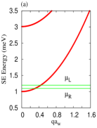
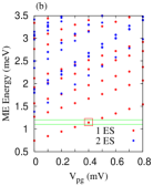
Figure 2: (Color online) Energy spectra in the case of no photon cavity with magnetic field $B=0.1$ T. (a) SE energy spectrum in the leads (red) is plotted as a function of wave number $q$, where the chemical potentials are $\mu_{L}=1.2\ {\rm meV}$ and $\mu_{R}=1.1\ {\rm meV}$ (green). (b) ME energy spectrum in the central system as a function of plunger gate voltage $V_{\rm pg}$ including SE states (1ES, red dots) and two electron states (2ES, blue dots). The SE state in the bias window is almost doubly degenerate due to the small Zeeman energy.

The SE state energy is tunable as a function of plunger gate voltage $V_{\rm pg}$ following $E_{\rm SE}(V_{\rm pg})=E_{\rm SE}(0)+eV_{\rm pg}$. We rank the SE and ME states by energy. In the absence of plunger gate voltage, the lowest active SE states in the central system are $|4)$ and $|5)$ with energies $E_{\rm 4}(0)=0.741$ meV and $E_{\rm 5}(0)=0.744$ meV, respectively. These two SE states may enter the chemical potential window $[\mu_{L},\mu_{R}]=[1.1,1.2]$ meV by tuning the plunger gate voltage to be $V_{\rm pg}\approx[0.35,0.45]\ {\rm mV}$. Consequently, the SE states occupying the first subband in the left lead are allowed to tunnel into the central ME system making resonant tunneling from the left to the right lead manifesting a main-peak feature in charging current $I_{Q}=0.112$ nA at $V_{\rm pg}=0.4\ {\rm mV}$ as shown in Fig. 3.

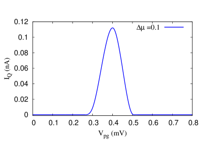
Figure 3: (Color online) The net charging current $I_{Q}$ is plotted as a function of plunger gate voltage $V_{\rm pg}$ at time $t=220$ ps in the case of no photon cavity. Other parameters are $B=0.1~{}{\rm T}$ and $\Delta\mu=0.1~{}{\rm meV}$.

In Fig. 4, we show the time evolution of the left and right partial charging currents in the case with no photon cavity to understand better how the $|4)$ and $|5)$ SE states in the bias window as well as the ground state with two electrons $|10)$ contribute to the transport. The state $|10)$ contributes because the energy difference $E_{10}-E_{4}$ (which includes the charging energy) is also in the bias window. In the short-time regime at $t=40$ ps, the partial current through the three active ME states are $I_{L,4}=0.852$ nA and $I_{R,4}=0.1$ nA through the state $|4)$ (red lines), $I_{L,5}=0.906$ nA and $I_{R,5}=0.121$ nA through the state $|5)$ (blue lines), and $I_{L,10}=0.002$ nA and $I_{R,10}=-0.025$ nA through the state $|10)$ (black lines). As a result, the net partial current contributed by the three active SE and ME states are $I_{4}=0.952$ nA, $I_{5}=1.027$ nA, $I_{10}=-0.023$ nA resulting in $I_{Q}=1.956$ nA. In the long-time regime at $t=220$ ps, $I_{L,4}=0.125$ nA and $I_{R,4}=0.12$ nA through the state $|4)$ (red lines), $I_{L,5}=-0.031$ nA and $I_{R,5}=-0.019$ nA through the state $|5)$ (blue lines), and $I_{L,10}=0.002$ nA and $I_{R,10}=-0.085$ nA through the state $|10)$ (black lines). The net partial charging current contributed by the three active ME states are thus $I_{4}=0.245$ nA, $I_{5}=-0.05$ nA, and $I_{10}=-0.083$ nA, thereby leading to the net charging current $I_{Q}=0.112$ nA. This exactly agrees with the result shown in Fig. 3. In the short-time regime, the left partial current contributed by the states $|4)$ and $|5)$ is much large than the right partial current. This illustrates significant charge accumulation in the short-time regime and, hence, manifests a broad peak structure as shown in Fig. 4

Figure 4: (Color online) Partial currents as a function of time without photon cavity: $I_{L}$ (red solid) and $I_{R}$ (red dashed) through the state $|4)$; $I_{L}$ (blue solid) and $I_{R}$ (blue dashed) through the state $|5)$. Other parameters are $V_{\rm pg}=0.4$ mV, $\Delta\mu=0.1~{}{\rm meV}$, $B=0.1~{}{\rm T}$, and $\hbar\Omega_{0}=2.0~{}{\rm meV}$.

In order to understand the nature of the electrons traversing the QD-embedded system, the distribution of ME charge is presented in Fig. 5 in the short time regime $40~{}{\rm ps}$ (left panel) and the long time regime $t=220~{}{\rm ps}$ (right panel) where the chemical potential difference is $\Delta\mu=0.1$ meV. In the short-time regime, the electrons in the QD-embedded system exhibits longitudinal oscillations. Two localized peaks are found located at the edges in the transport direction of the embedded QD due to the breaking of the translational invariance at the edges of the embedded QD, as shown in Fig. 5(a), that favors the electrons making coherent elastic multiple scattering. In the long-time regime, a broader bound state with a long tail in the transport direction is found that corresponds to the resonant state in the finite wire system. In the following sections, we shall place the QD system in a photon cavity with a single-photon mode. We shall analyze the transient transport properties for the cases with linear polarizations in either $x$ or $y$ directions.

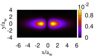
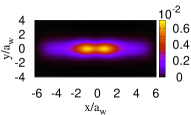
Figure 5: (Color online) The spatial distribution of the ME charge density at short-time $t=40$ ps (left panel) and long-time $t=220$ ps (right panel) in the case with no photon cavity, where the plunger gate is $V_{\rm pg}=0.4$ meV. Other parameters are $B=0.1$ T, $a_{w}$ = $23.8~{}{\rm nm}$, $L_{x}$ = $300$ nm = $12.6a_{w}$, and $\Delta\mu=0.1~{}{\rm meV}$.

III.2 $x$-polarized photon mode

Here, we demonstrate how the QD embedded in a quantum wire can be controlled by the plunger-gate and how it is influenced by the photon field, where the electric field of the TE₀₁₁ mode is polarized in the $x$-direction. The initial condition of the system under investigation is an empty central system (no electron) that is coupled to a single-photon mode with one photon present, connected to the leads with a source-drain bias. The MB energy spectrum of the electron-photon interacting MB system is illustrated in Fig. 6. As shown in the previous section, active states get into the bias window around $V_{\rm pg}^{0}=0.4$ mV in the case with no photon cavity. It is interesting to note that additional active states can be included around $eV_{\rm pg}=eV_{\rm pg}^{0}\pm\hbar\omega_{\rm ph}$ as is clearly seen in Fig. 6, this implies that the $x$-polarized photon-field induced active propagating states can be found around $V_{\rm pg}=0.1$ and $0.7$ mV when the photon energy is $\hbar\omega_{\rm ph}=0.3$ meV. The additional photon-induced propagating states play an important role to enhance the electron tunneling from the leads to the QD system.

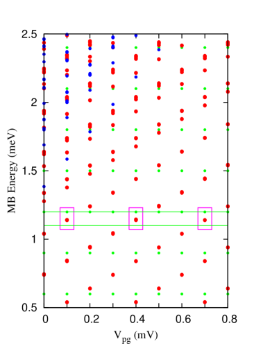
Figure 6: (Color online) MB Energy spectrum versus the plunger gate voltage $V_{\rm pg}$ in the case of $x$-polarized photon field, where zero electron states ($N_{e}=0$, green dots), single-electron states ($N_{e}=1$, red dots), and two-electron states ($N_{e}=2$, blue dots) are included. Other parameters are $B=0.1$ T, $\Delta\mu=0.1$ meV, and $\hbar\omega_{\rm ph}=0.3~{}{\rm meV}$.

Figure 7 shows the net charging current $I_{Q}$ as a function of the plunger-gate voltage $V_{\rm pg}$ in the presence of the $x$-polarized photon field at time $t=220$ ps. We fix the photon energy at $\hbar\omega_{\rm ph}=0.3~{}{\rm meV}$ and change the electron-photon coupling strength $g_{\rm ph}$. A main peak around $V_{\rm pg}^{0}=0.4$ mV is found, a robust left side peak around $eV_{\rm pg}=eV_{\rm pg}^{0}-\hbar\omega_{\rm ph}$ is clearly shown, and a right side peak around $eV_{\rm pg}=eV_{\rm pg}^{0}+\hbar\omega_{\rm ph}$ can be barely recognized. The left side peak exhibits photon-assisted transport feature from the SE MB states $|\breve{20})$ and $|\breve{22})$ in the bias window by absorbing a photon energy $\hbar\omega_{\rm ph}$ to the SE MB states $|\breve{26})$ and $|\breve{28})$ above the bias window. However, the opposite photon-assisted transport feature caused by a photon emission (the right side peak) is significantly suppressed.

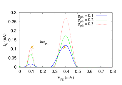
Figure 7: (Color online) The net charging current $I_{Q}$ versus the plunger gate voltage $V_{\rm pg}$ in the case of $x$-polarized photon field at time $t=220~{}{\rm ps}$ with different electron-photon coupling strength: $g_{\rm ph}=0.1$ meV (blue solid), $g_{\rm ph}=0.2$ meV (green dashed), and $g_{\rm ph}=0.3$ meV (red dotted). Other parameters are $\hbar\omega_{ph}=0.3~{}{\rm meV}$, $\Delta\mu=0.1~{}{\rm meV}$, and $B=0.1~{}{\rm T}$.

The main charge current peaks for $V_{\rm pg}=0.4$ mV are $I_{Q}^{M}=0.120,0.173$, and $0.270$ nA corresponding to $g_{\rm ph}=0.1~{}{\rm meV}$, (blue solid), $g_{\rm ph}=0.2~{}{\rm meV}$ (green dashed), and $g_{\rm ph}=0.3~{}{\rm meV}$ (red dotted) as shown in Fig. 7. Our results demonstrate that the current carried by the electrons with energy within the bias window can be strongly enhanced by increasing the electron-photon coupling strength. At $V_{\rm pg}=0.1$ mV, the left side peaks in the charging current are $I_{Q}^{S}=0.017,0.072$, and $0.103$ nA corresponding to $g_{\rm ph}=0.1,0.2$, and $0.3$ meV. This implies that the electrons may absorb a single-photon energy and, hence, the charging current manifests a photon-assisted transport.

To identify the active MB states contributing to the transient transport, we show the characteristics of the MB states at $V_{\rm pg}=0.4$ and 0.1 meV in Fig. 8(a) and (b) corresponding, respectively, to the main peak and the left side peak in $I_{Q}$ shown in Fig. 7. More precisely, there are five MB states contributing to the main peak in $I_{Q}$ at $V_{\rm pg}=0.4$ meV. The five active MB states are: $|\breve{17})$ and $|\breve{18})$ with energies $E_{17}=1.143$ meV and $E_{18}=1.145$ meV in the bias window ($N_{e}=1$, $N_{\rm ph}=0.04$), $|\breve{21})$, $|\breve{23})$ with energies $E_{21}=1.439$ meV and $E_{23}=1.441$ meV above the bias window ($N_{e}=1$, $N_{\rm ph}=0.96$) shown in Fig. 8(a), and $|\breve{53})$ with energy $2.488$ meV (not shown). It is interesting to notice that $E_{17}+\hbar\omega_{\rm ph}\cong E_{21}$ and $E_{18}+\hbar\omega_{\rm ph}\cong E_{23}$, this implies a photon-assisted transport through the higher MB states.

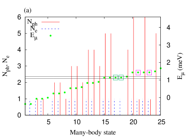
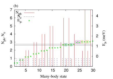
Figure 8: (Color online) The MB energy spectrum $E_{\mu}$ (dotted green), the mean electron number in the MB state $|\breve{\mu})$ (blue dashed line), the mean photon number $N_{\rm ph}$ (red line) in the case of $x$-polarized field: (a) $V_{\rm pg}=0.4$ meV and (b) $V_{\rm pg}=0.7$ meV. Other parameters are $B=0.1~{}{\rm T}$, $\Delta\mu=0.1~{}{\rm meV}$, $g_{\rm ph}=0.1$ meV, $\hbar\omega_{\rm ph}=0.3$ meV.

When an electron enters the QD system it interacts with the photon in the cavity. Its energy is thus not in resonance with the electron states in the bias window, but with the electron states, photon replicas, which are a with photon energy $\hbar\omega_{ph}$ above the states in the bias window. The photon activated states above the bias contain approximately one more photon than the states in the bias window and, hence, the main-peak in $I_{Q}$ is mainly due to a single-photon absorption mechanism. In addition to the main-peak feature at plunger-gate voltage $V^{\rm M}_{\rm pg}$, two side peaks can be recognized at $eV^{\rm S}_{\rm pg}=eV^{\rm M}_{\rm pg}\pm\hbar\omega_{\rm ph}$ induced by a photon-assisted transport, where the system satisfies $e\Delta V^{\rm MS}_{\rm pg}=e|V^{\rm M}_{\rm pg}-V^{\rm S}_{\rm pg}|\cong\hbar\omega_{\rm ph}$. It has been pointed out that this plunger-gate controlled photon-assisted transport is repeatable with period related to the Coulomb charging energy.Kouwenhoven et al. (1994b)

Figure 8(b) shows how the left-side peak in the net charging current $I_{Q}$ shown previously in Fig. 7 is contributed by the MB states. First, the left current $I_{L}=0.001$ nA and the right current $I_{R}=-0.001$ nA contributed by the $|\breve{20})$ and $|\breve{22})$ MB states (green squared dot) containing $N_{\rm e}=1$ and $N_{\rm ph}=0.96$ within the bias window are almost negligible, this implies the left side peak in $I_{Q}$ is not induced by the resonant tunneling effect. Second, the $|\breve{24})$ and $|\breve{25})$ MB states (pink squared dot) contain $N_{\rm e}=1$ and $N_{\rm ph}=0.04$ with energies $E_{24}=1.376$ meV and $E_{25}=1.379$ meV, above the bias window. These two states contribute, respectively, to the charging current $I_{24}=0.0$ nA ($I_{L,24}=0.003$ nA, $I_{R,24}=-0.003$ nA) and $I_{25}=0.001$ nA ($I_{L,25}=0.007$ nA, $I_{R,25}=-0.006$ nA) and, hence, generate a charging current $I_{Q}^{c}=0.001$ nA. Third, the $|\breve{26})$ and $|\breve{28})$ MB states (orange squared dot) contain $N_{\rm e}=1$ and $N_{\rm ph}=1.96$ with energies $E_{26}=1.435$ meV and $E_{28}=1.438$ meV above the bias window. These two states contribute, respectively, to the charging current $I_{26}=0.01$ nA ($I_{L,26}=0.010$ nA, $I_{R,26}=0.0$ nA) and $I_{28}=0.004$ nA ($I_{L,28}=0.005$ nA, $I_{R,28}=-0.001$ nA) and, hence generate a photon-assisted tunneling current $I_{Q}^{\rm ph}=0.014$ nA. The main contribution of the left side peak in the charging current is then $I_{Q}\approx I_{Q}^{c}+I_{Q}^{\rm ph}=0.015$ nA, this coincides with the result shown in Fig. 7.

The schematic diagram in Fig. 9 is shown to illustrate the dynamical photon-assisted transport processes involved in the formation of the main peak and the left side peak in the net charging current $I_{Q}$ shown in Fig. 7. It is illustrated in Fig. 9(a) that the transport mechanism forming the main peak in $I_{Q}$ is mainly due to the photon-assisted tunneling to the MB states above the bias window containing approximately a single photon. Figure 9(b) represents two main transport mechanisms forming the left side peak in $I_{Q}$. The electrons in the left lead may absorb two photons to the MB states containing approximately two photons above the bias window. After that, the electrons may either perform resonant tunneling to the right lead (red solid arrow) or make multiple inelastic scattering by absorbing and emitting photon energy $\hbar\omega_{\rm ph}$ in the QD system (blue dashed arrow). This is the key result of this paper.

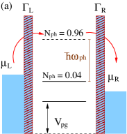
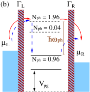
Figure 9: (Color online) Schematic representation of photon activated resonance energy levels and electron transition by changing the plunger gate voltage $V_{\rm pg}$ at the main peak (a) and the left side peak (b) in Fig. 7. The QD system is embedded in a photo cavity with the photon energy $\hbar\omega_{\rm ph}$ and photon content $N_{\rm ph}$ in each many-body state. The chemical potential difference is $\Delta\mu=\mu_{L}-\mu_{R}$, and $\Gamma_{\rm{L,R}}$ is the coupling strength between the QD system and the leads.

To get better insight into the dynamical electronic transport, the spatial distribution of the ME charge at $t=220$ ps is shown in Fig. 10. Similar to the QD system in the absence of the photon cavity, the ME charge distribution at the main-peak in $I_{Q}$ forms resonant peaks at the edges of the QD, as shown Fig. 10(a), that is related to an antisymmetric state in the QD. The partial occupation contributed by the photon activated resonant MB states $|\breve{21})$ and $|\breve{23})$ are $0.432e$ and $0.454e$, respectively. Comparing to the case with no photon cavity, the slight enhancement in the ME charge indicates that the tunneling of electrons into the QD system becomes faster in the presence of the photon cavity and, hence, the charging current is enhanced. It is shown in Fig. 10(b) that the ME charge in the case of side peak in $I_{Q}$ manifests an extended SE state, which is formed outside the QD. The partial occupation contributed by the photon activated resonant MB states $|\breve{24})$ and $|\breve{25})$ are $0.018e$ and $0.025e$, respectively. By increasing the photon energy $\hbar\omega_{\rm ph}$, the left side peak in $I_{Q}$ can be enhanced and is shifted to lower energy (not shown). The slight asymmetry seen in the charge distribution in Fig. 10(b) is caused by the $x$-polarized electric field of the photons.

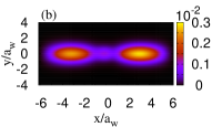
Figure 10: (Color online) The spatial distribution of the many-electron charge density of the QD system with $x$-polarized photon field at time $220$ ps corresponding to the main peak (a) and the left side peak (b) for the case of $g_{\rm ph}=0.1$ meV shown in the Fig. 7 (blue solid line). Other parameters are $\hbar\omega_{\rm ph}=0.3~{}{\rm meV}$, $B=0.1$ T, $a_{w}=23.8~{}{\rm nm}$, $L_{x}=300~{}{\rm nm}$, and $\hbar\Omega_{0}=2.0~{}{\rm meV}$.

III.3 $y$-polarized photon mode

We consider here the TE₁₀₁ $y$-polarized photon mode, where the electric field of the photons is perpendicular to the transport direction through the QD system. The QD system is assumed to be initially containing no electron $N_{e}=0$, but one photon in the cavity $N_{\rm ph}=1$. Since our system is considered to be anisotropic, elongated in the $x$-direction, we shall demonstrate that the photon-assisted transport effect is much weaker in the case of a $y$-polarized photon mode in comparison with that of $x$-polarization discussed in the previous section.

In Fig. 11, we present the MB energy spectrum as a function of plunger-gate voltage $V_{\rm pg}$ for a QD system influenced by the $y$-polarized field with photon energy $\hbar\omega_{\rm ph}=0.3~{}{\rm meV}$. Besides the propagating state at $V_{\rm pg}=0.4$ mV within the bias window (green lines), there are two additional electronic propagating states appearing at $V_{\rm pg}=0.1$ and 0.7 mV caused by the presence of the photon field as marked by the squared dots shown in the figure.

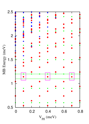
Figure 11: (Color online) MB energy spectrum versus the plunger-gate voltage $V_{\rm pg}$ in the case of $y$-polarized photon field: zero-electron states $N_{e}=0$ (green dots), single-electron states $N_{e}=1$ (red dots), and two-electron states $N_{e}=2$ (blue dots). Other parameters are $B=0.1$ T, $\Delta\mu=0.1$ meV, $\hbar\Omega_{0}=2.0$ meV, $\hbar\omega_{\rm ph}=0.3~{}{\rm meV}$, and $g_{\rm ph}=0.1$.

Figure 12 shows the net charging current in the case of $y$-polarized photon field, in which there is initially one photon $N_{\rm ph}=1$ with energy $\hbar\omega_{\rm ph}=0.3~{}{\rm meV}$ fixed while the electron-photon coupling strength is changed. It is seen that main peak currents at $V_{\rm pg}=0.4$ mV are: $I_{Q}^{M}=0.115$ nA for $g_{\rm ph}=0.1$ meV (blue solid), $I_{Q}^{M}=0.127$ nA for $g_{\rm ph}=0.2$ meV (green dashed), and $I_{Q}^{M}=0.159$ nA for $g_{\rm ph}=0.3$ meV (red dotted). Moreover, weak left side-peak current at $V_{\rm pg}=0.1$ mV can be recognized: $I_{Q}^{S}=1.0$ pA for $g_{\rm ph}=0.1$ meV, $I_{Q}^{S}=1.7$ pA for $g_{\rm ph}=0.2$ meV, and $I_{Q}^{S}=3.2$ pA for $g_{\rm ph}=0.3$ meV. We notice that both the side and main peak currents are enhanced when the electron-photon coupling strength is increased. In order to get better understanding of the current enhancement, we repeat the analysis of the photon activated MB energy states contributing to the electronic transport.

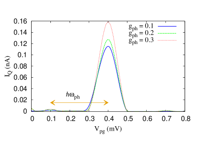
Figure 12: (Color online) net charging current versus the plunger gate voltage $V_{\rm pg}$ at time ($t=220~{}{\rm ps}$) in the case of $y$-polarized photon field. The electron-photon coupling is changed to be $g_{\rm ph}=0.1$ meV (blue solid), $g_{\rm ph}=0.2$ meV (green dashed), and $g_{\rm ph}=0.3$ meV (red dotted). Other parameters are $\hbar\omega_{\rm ph}=0.3~{}{\rm meV}$, $\Delta\mu=0.1~{}{\rm meV}$, and $B=0.1~{}{\rm T}$.

In Fig. 13(a), we show the MB states at $V_{\rm pg}=0.4$ mV and $g_{\rm ph}=0.1$. The active MB states are $|\breve{16})$ and $|\breve{18})$ with energies 1.141 and 1.144 meV in the bias window ($N_{\rm ph}=0$), $|\breve{21})$ and $|\breve{23})$ with energies 1.441 and 1.444 meV above the bias window ($N_{\rm ph}=1$), and $|\breve{53})$ with energy 2.483 meV ($N_{\rm ph}=1$). It should be noticed that $E_{16}+\hbar\omega_{\rm ph}\cong E_{21}$ and $E_{18}+\hbar\omega_{\rm ph}\cong E_{23}$ indicating that these two MB states above the bias window are photon-activated states. Furthermore, the higher active MB state with energy approximately the same with the characteristic Coulomb energy, that is $E_{53}\approx E_{\rm C}$, indicates a correlation induced active two-electron state.

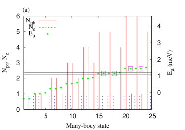
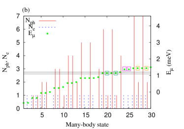
Figure 13: (Color online) The many-body energy spectrum $E_{\mu}$ (dotted green), the mean electron number in the many-body state $|\breve{\mu})$ (blue dashed line), the mean photon number $N_{ph}$ (red line) of the main peak $V_{\rm pg}=0.4$ meV (a), and the left side peak $V_{\rm pg}=0.1$ meV (b). The magnetic fields $B=0.1~{}{\rm T}$, $\Delta\mu=0.1~{}{\rm meV}$, $g_{\rm ph}=0.1$ meV, $\hbar\omega_{\rm ph}=0.3$ meV. In the case of $y$-polarized photon field.

The net charging current at $V_{\rm pg}=0.4$ mV exhibiting the main current peak in Fig. 12 at $t=220$ ps is mainly contributed by the MB states $|\breve{21})$ ($I_{L,21}=0.127$ nA, $I_{R,21}=0.125$ nA) and $|\breve{23})$ ($I_{L,23}=-0.032$ nA, $I_{R,23}=-0.018$ nA). This indicates that the electrons in the left lead can absorb one photon to the state $|\breve{21})$ and then emit one photon preforming resonant tunneling to the right lead, and contribute to the charging current $I_{21}=0.252$ nA. Moreover, an opposite transport mechanism can happen for the electrons in the right lead through the state $|\breve{23})$, and then contribute to the charging current $I_{23}=-0.05$ nA. The scattering processes through these two states results in a photon-assisted tunneling current $I_{Q}^{\rm ph}=0.202$ nA. A small current through $|\breve{53})$ is found due to the charging effect, namely $I_{L}=0.002$ nA and $I_{R}=-0.087$ nA, and hence contribute to the charging current $I_{Q}^{c}=-0.085$ nA due to charging effect. The contribution to the main peak in charging current is therefore $I_{Q}\approx I_{Q}^{\rm ph}+I_{Q}^{c}$ = $0.117$ nA. This analysis is consistent with the result shown in Fig. 12.

In Fig. 13(b), we show the MB states at $V_{\rm pg}=0.1$ mV and $g_{\rm ph}=0.1$. The active MB states are: $|\breve{20})$ and $|\breve{22})$ with energies $E_{20}=1.141$ meV and $E_{22}=1.144$ meV in the bias window ($N_{\rm ph}=1$); $|\breve{24})$ and $|\breve{25})$ with energies 1.368 and 1.371 meV above the bias window ($N_{\rm ph}=0$); and $|\breve{27})$ and $|\breve{29})$ with energy $E_{27}=1.441$ meV and $E_{29}=1.444$ meV ($N_{\rm ph}=2$). We notice that $E_{20}+\hbar\omega_{\rm ph}\cong E_{27}$ and $E_{22}+\hbar\omega_{\rm ph}\cong E_{29}$. This implies that the two MB states $|\breve{27})$ and $|\breve{29})$ above the bias window are photon-activated states.

In Fig. 12, the net charging current at $V_{\rm pg}=0.1$ mV manifests a small side-peak current $I_{Q}^{S}=1.0$ pA at $t=220$ ps. This left side-peak structure in $I_{Q}$ is mainly contributed by the MB states $|\breve{20})$ ($I_{L}=1.1$ pA, $I_{R}=-0.9$ pA) and $|\breve{22})$ ($I_{L}=1.2$ pA, $I_{R}=-0.9$ pA) in the bias window. These two states contribute to the resonant tunneling current, $I_{Q}^{r}=0.5$ pA, that is related to the charge accumulation effect. In addition, the states $|\breve{27})$ ($I_{27}=4\times 10^{-3}$ pA) and $|\breve{29})$ ($I_{29}=2\times 10^{-3}$ pA) contribute to very weak charging current $I_{Q}^{\rm ph}=6\times 10^{-3}$ pA due to photon-assisted tunneling. The contribution to the side-peak current is therefore $I_{Q}^{S}\approx I_{Q}^{r}+I_{Q}^{\rm ph}$ = $0.51$ pA. The suppression of the side-peak current in the case of $y$-polarization is due to the anisotropy of our system. The dipole momentum in the $y$-direction is much smaller in the $x$-direction, and so is the electron-photon interaction strength.

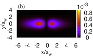
Figure 14: (Color online) The spatial distribution of the ME charge density in the case of $y$-polarized photon field at time $220$ ps: (a) $V_{\rm pg}=0.4$ mV and (b) $V_{\rm pg}=0.1$ mV corresponding, respectively, to the main peak and the left side peak in Fig. 12 (blue line, $g_{\rm ph}=0.1$ meV). Other parameters are $\hbar\omega_{\rm ph}=0.3~{}{\rm meV}$, $B=0.1$ T, $a_{w}=23.8~{}{\rm nm}$, $L_{x}=300~{}{\rm nm}$, and $\hbar\Omega_{0}=2.0~{}{\rm meV}$.

The ME charge distribution in the presence of the $y$-polarized photon mode is shown in Fig. 14. It is seen that the main-peak current in Fig. 12 forms an elongated broad bound state in the central system due to the electron-photon interaction as shown in Fig. 14(a). Moreover, the side-peak current in Fig. 12 forms a photon-assisted resonant state at the edges of the QD embedded in the quantum wire, as is shown in Fig. 14(b). We notice that the charge distribution maxima around $x\approx\pm a_{w}$ of the main peak in $I_{Q}$ at $V_{\rm pg}=0.4$ mV with $g_{\rm ph}=0.1$ meV are almost the same in the cases without and with photon mode. As a consequence, the main-peak current $I_{Q}^{M}\simeq 0.1$ nA for theses cases. Furthermore, the charging current maxima are located around $x\approx\pm 3a_{w}$ in the case of $x$-polarization while located around $x\approx\pm 2a_{w}$ in the case of $y$-polarization. The charge distribution maxima in the case of $x$-polarization is closer to the edges of the central system implying the higher left side-peak current at $V_{\rm pg}=0.1$ mV.

IV Concluding Remarks

We have performed numerical calculation to investigate the transient current and charge distribution of electrons through a QD embedded in a finite wire coupled to a single-photon mode with $x$- or $y$-polarization. A non-Markovian theory is utilized where we solve a generalized QME that includes the electron-electron Coulomb interaction and electron-photon coupling. Initially, we examine the case without a photon cavity. In the short-time regime, the charging current exhibits significant charge accumulation effect. In the long-time regime, the charging current is suppressed due to the Coulomb blocking effect. Furthermore, we have analyzed the photon-assisted current and the characteristics of photon activated MB states with various parameters coupled to single-photon mode in the photon cavity. The photon-assisted current peaks are enhanced by increased electron-photon coupling strength.

In the case of a QD system coupled to an $x$-polarized photon mode, the main current peak is enhanced by the electron-photon coupling. The electrons may absorb a single photon manifesting a photon-assisted secondary peak which also incorporates correlation effects. In the case of a QD coupled to a $y$-polarized photon mode, the main current peak is contributed to by two photon-activated single-electron states and a correlation-induced two-electron state. The secondary peak current in the case of $y$-polarization is suppressed due to the anisotropy of our system.

The cavity photon assisted or enhanced transport here was attainable by selecting a narrow bias window in order to facilitate the resonant placement and isolation of spin-pair of states with a single-electron component by the plunger gate in the bias window. The bias window was kept in the lowest part of the MB energy spectrum and the low photon energy guarantees in most cases that only states close to this very descrete part of the spectrum are relevant to the transport. This is in contrast to our experience with large bias window where the coupling to the cavitiy photons most often reduce the charging of the central system.Gudmundsson et al. (2012, 2013); Arnold et al. (2013)

Our proposed plunger-gate controlled transient current in a single-photon-mode influenced QD system should be observable due to recent rapid progress of measurement technology.F$\grave{\rm e}$ve et al. (2007) The realization of a single-photon influenced QD device and the generation of plunger-gate controlled transient transport may be useful in quantum computation applications.